
Hitoshi Murayama, Unified Field Theories, Encyclopedia of Applied Physics, Vol. 23, 1 (1998)

UNCERTAINTY THEORIES: A UNIFIED VIEW
D. Dubois IRIT-CNRS, Université Paul Sabatier
31062 TOULOUSE FRANCE

Outline 1. Variability vs ignorance 2. Set-valued representations of ignorance, vs.
representations of real sets 3. Blending set-valued and probabilistic
representations : uncertainty theories 4. Comparison of uncertainty theories on
1. Practical representations 2. Information content 3. Conditioning 4. Combination

Origins of uncertainty • The variability of observed natural phenomena :
randomness. – Coins, dice…: what about the outcome of the next
throw? • The lack of information: incompleteness
– because of information is often lacking, knowledge about issues of interest is generally not perfect.
• Conflicting testimonies or reports: inconsistency – The more sources, the more likely the inconsistency

Example • Frequentist: daily quantity of rain in Toulouse
– Represents variability: it may change every day – It is objective: can be estimated through statistical data
• Incomplete information : Birth date of Brazilian President – It is not a variable: it is a constant! – Information is incomplete – It subjective: Most may have a rough idea (an interval), a few
know precisely, some have no idea. – Statistics on birth dates of other presidents do not help much.

Knowledge vs. evidence • There are two kinds of information that help us make
decisions in the course of actions: – Generic knowledge:
• pertains to a population of observables (e.g. statistical knowledge) • Describes a general trend based on objective data • Tainted with exceptions • Deals with observed frequencies or ideas of typicality
– Singular evidence: • Consists of direct information about the current world. • pertains to a single situation • Can be unreliable, uncertain (e.g. unreliable testimony)

The roles of probability
Probability theory is generally used for representing two types of phenomena:
1. Randomness: capturing variability through repeated observations.
2. Belief: describes a person’s opinion on the occurrence of a singular event.
As opposed to frequentist probability, subjective probability that models unreliable evidence is not necessarily related to statistics.

Constructing beliefs
• Belief in the occurrence of a particular event may derive from its statistical probability: the Hacking principle: – Generic knowledge = probability distribution P – beliefNOW(A) = FreqPOPULATION(A): equating belief and frequency
• Beliefs can be directly elicited as subjective probabilities of singular events with no frequentist flavor – frequencies may not be available nor known – non repeatable events.
• But a single subjective probability distribution cannot distinguish between uncertainty due to variability and uncertainty due to lack of knowledge

SUBJECTIVE PROBABILITIES (Bruno de Finetti, 1935)
• pi = belief degree of an agent on the (next) occurrence of si • measured as the price of a lottery ticket with reward 1 € if
state is si in a betting game • Rules of the game:
– gambler proposes a price pi – banker and gambler exchange roles if banker finds price
pi is too low • Why a belief state is a single distribution (∑j pj= 1):
– Assume player buys all lottery tickets i = 1, m. – If state sj is observed, the gambler gain is 1 – ∑j pj – and ∑j pj– 1 for the banker – if ∑pj > 1 gambler always loses money ; – if ∑pj < 1 banker exchanges roles with gambler

Using a single probability distribution to represent incomplete information is not entirely satisfactory:
The betting behavior setting of Bayesian subjective probability enforces a representation of partial ignorance based on single probability distributions.
1. Ambiguity : In the absence of information, how can a uniform diistribution tell pure randomness and ignorance apart ?
2. Instability : A uniform prior on x∈ [a, b] induces a non-uniform prior on f(x) ∈ [f(a), f(b)] if f is increasing and non-affine.
3. Empirical refutation: When information is missing, decision-makers do not always choose according to a single subjective probability (Ellsberg paradox).

Motivation for going beyond probability
• Distinguish between uncertainty due to variability from uncertainty due to lack of knowledge or missing information.
• The main tools to representing uncertainty are – Probability distributions : good for expressing variability, but
information demanding
– Sets: good for representing incomplete information, but often crude representation of uncertainty
• Find representations that allow for both aspects of uncertainty.

Set-Valued Representations of Partial Knowledge
• An ill-known quantity x is represented as a disjunctive set, i.e. a subset E of mutually exclusive values, one of which is the real one.
• Pieces of information of the form x ∈ E – Intervals E = [a, b]: good for representing incomplete
numerical information – Classical Logic: good for representing incomplete
symbolic (Boolean) information E = Models of a wff φ stated as true.
This kind of information is subjective (epistemic set)

BOOLEAN POSSIBILITY THEORY Natural set functions under incomplete information: If all we know is that x ∈ E then - Event A is possible if A ∩ E ≠ Ø (logical consistency) Π(A) = 1, and 0 otherwise
- Event A is sure if E ⊆ A (logical deduction) N(A) = 1, and 0 otherwise
This is a simple modal logic (KD45) N(A) = 1 - Π(Ac)
Π(A ∪ B) = max(Π(A), Π(B)); N(A ∩ B) = min(N(A), N(B)).
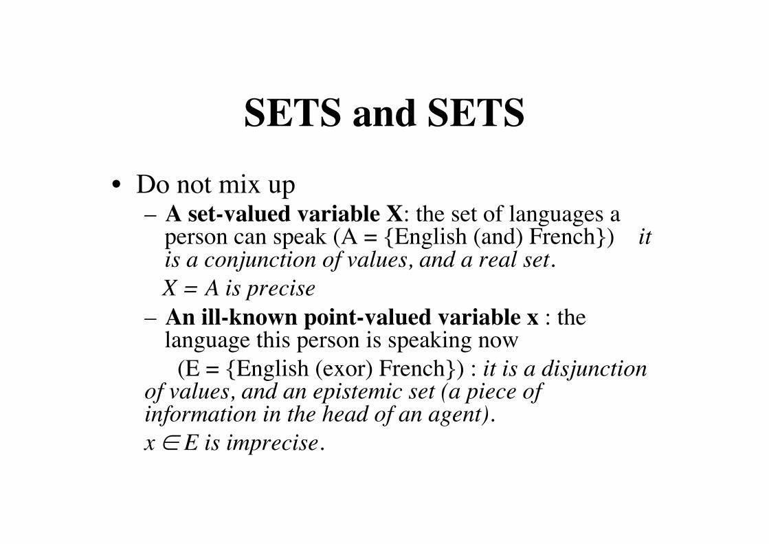
SETS and SETS • Do not mix up
– A set-valued variable X: the set of languages a person can speak (A = English (and) French) it is a conjunction of values, and a real set.
X = A is precise – An ill-known point-valued variable x : the
language this person is speaking now (E = English (exor) French) : it is a disjunction
of values, and an epistemic set (a piece of information in the head of an agent). x ∈ E is imprecise.

Find a representation of uncertainty due to incompleteness
• More informative than sets • Less demanding than single probability
distributions • Explicitly allows for missing information • Allows for addressing the same problems as
probability.

Blending intervals and probability
• Representations that may account for both variability and incomplete knowledge must combine probability and sets. – Sets of probabilities : imprecise probability theory – Random(ised) sets : Dempster-Shafer theory – Fuzzy sets: numerical possibility theory
• Each event has a degree of belief (certainty) and a degree of plausibility, instead of a single degree of probability

A GENERAL SETTING FOR REPRESENTING GRADED CERTAINTY AND PLAUSIBILITY
• 2 conjugate set-functions Pl and Cr generalizing probability P, possibility Π, and necessity N.
• Conventions : – Pl(A) = 0 "impossible" ; Cr(A) = 1 "certain" – Pl(A) =1 ; Cr(A) = 0 "ignorance" (no information) – Pl(A) - Cr(A) quantifies ignorance about A
• Postulates – Cr and Pl are monotonic under inclusion (= capacities). – Cr(A) ≤ Pl(A) "certain implies plausible" – Pl(A) = 1 - Cr(Ac) duality certain/plausible – If Pl = Cr then it is P.

Possibility Theory (Shackle, 1961, Zadeh, 1978)
• A piece of incomplete information "x ∈ E" admits of degrees of possibility: E is a (normalized) fuzzy set.
• µE(s) = Possibility(x = s) = πx(s) • Conventions: ∀s, πx(s) is the degree of plausibility of x = s πx(s) = 0 iff x = s is impossible, totally surprising πx(s) = 1 iff x = s is normal, fully plausible, unsurprising (but no certainty)

A pioneer of possibility theory • In the 1950’s, G.L.S. Shackle called "degree of potential
surprize" of an event its degree of impossibility = 1 - Π(Α).
• Potential surprize is valued on a disbelief scale, namely a positive interval of the form [0, y*], where y* denotes the absolute rejection of the event to which it is assigned, and 0 means that nothing opposes to the occurrence of A.
• The degree of surprize of an event is the degree of surprize of
its least surprizing realization. • He introduces a notion of conditional possibility

Improving expressivity of incomplete information representations
• What about the birth date of the president? • partial ignorance with ordinal preferences : May have
reasons to believe that 1933 > 1932 ≡ 1934 > 1931 ≡ 1935 > 1930 > 1936 > 1929
• Linguistic information described by fuzzy sets: “ he is old ” : membership µOLD is ionterpreted as a possibility distribution on possible birth dates.
• Nested intervals E1, E2, …En with confidence levels N(Ei) = ai : ‒ π(x) = mini = 1, …n max (µEi(x), 1- ai)

POSSIBILITY AND NECESSITY
OF AN EVENT
How confident are we that x ∈ A ⊂ S ? (an event A occurs) given a possibility distribution on S
• Π(A) = maxs∈A π(s) : to what extent A is consistent with π
(= some x ∈ A is possible) The degree of possibility that x ∈ A • N(A) = 1 – Π(Ac) = min s∉A 1 – π(s):
to what extent no element outside A is possible = to what extent π implies A
The degree of certainty (necessity) that x ∈ A

Basic properties
Π(A ∪ B) = max(Π(A), Π(B)); N(A ∩ B) = min(N(A), N(B)).
Mind that most of the time : Π(A ∩ B) < min(Π(A), Π(B)); N(A ∪ B) > max(N(A), N(B)
Example: Total ignorance on A and B = Ac
Corollary N(A) > 0 ⇒ Π(A) = 1

Qualitative vs. quantitative possibility theories • Qualitative:
– comparative: A complete pre-ordering ≥π on U A well-ordered partition of U: E1 > E2 > … > En
– absolute: πx(s) ∈ L = finite chain, complete lattice... • Quantitative: πx(s) ∈ [0, 1], integers... One must indicate where the numbers come from. All theories agree on the fundamental maxitivity axiom Π(A ∪ B) = max(Π(A), Π(B))
Theories diverge on the conditioning operation

Imprecise probability theory • A state of information is represented by a family P
of probability distributions over a set X. • To each event A is attached a probability interval
[P*(A), P*(A)] such that – P*(A) = infP(A), P∈ P – P*(A) = supP(A), P∈ P = 1 – P*(Ac)
• Usually P is strictly contained in P(A), P ≥ P* • For instance: incomplete knowledge of an
objective probabilistic model : ∃ P ∈ P.

Subjectivist view (Peter Walley) • Plow(A) is the highest acceptable price for buying a
bet on singular event A winning 1 euro if A occurs • Phigh(A) = 1 – Plow(Ac) is the least acceptable price
for selling this bet. • Rationality conditions:
– No sure loss : P ≥ Plow not empty – Coherence: P*(A) = infP(A), P ≥ Plow = Plow(A)
• A theory that handles convex probability sets • Convex probability sets are actually characterized
by lower expectations of real-valued functions (gambles), not just events.

Random sets • A probability distribution m on the family
of non-empty subsets of a set S. • A positive weighting of non-empty subsets:
mathematically, a random set : ∑ m(E) = 1 E ∈ F
• m : mass function. • focal sets : E ∈F with m(E) > 0 :
disjunctive or conjunctive ???
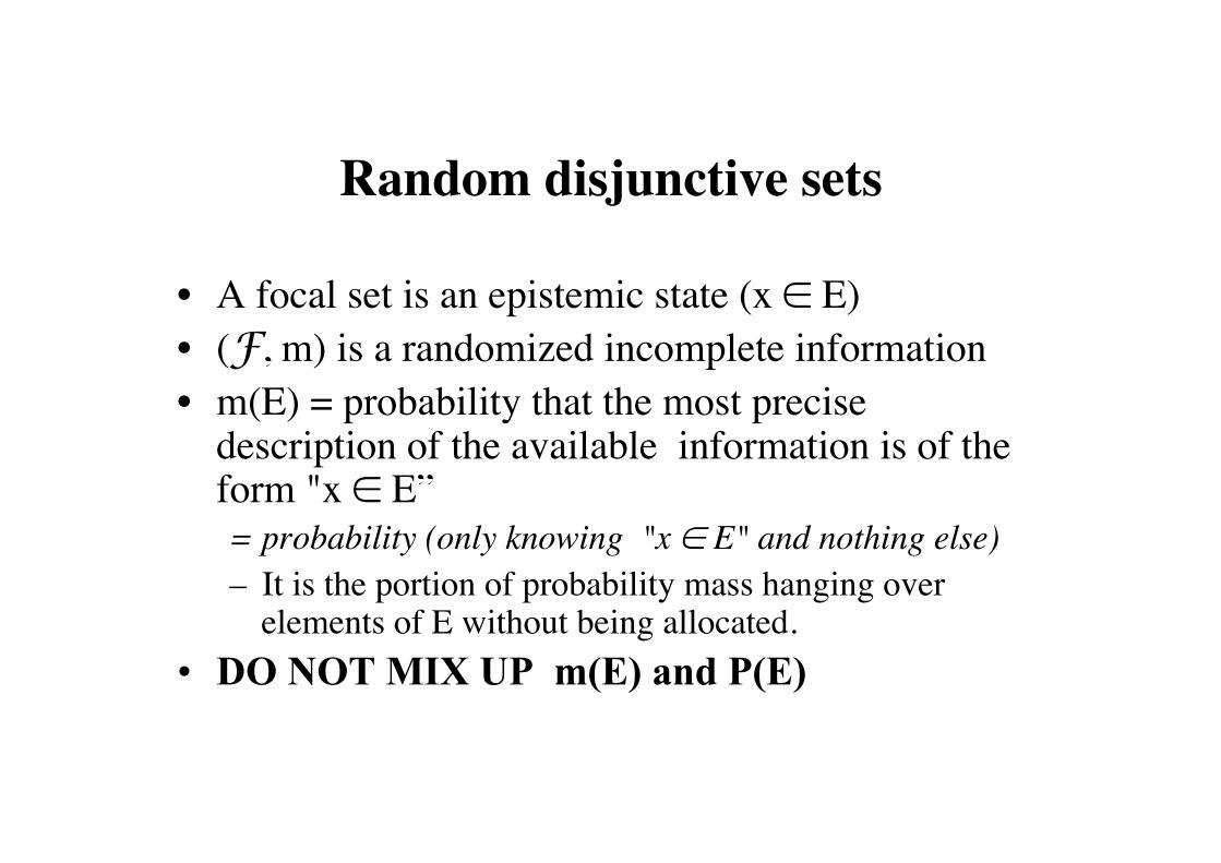
Random disjunctive sets
• A focal set is an epistemic state (x ∈ E) • (F, m) is a randomized incomplete information • m(E) = probability that the most precise
description of the available information is of the form "x ∈ E” = probability (only knowing "x ∈ E" and nothing else) – It is the portion of probability mass hanging over
elements of E without being allocated. • DO NOT MIX UP m(E) and P(E)
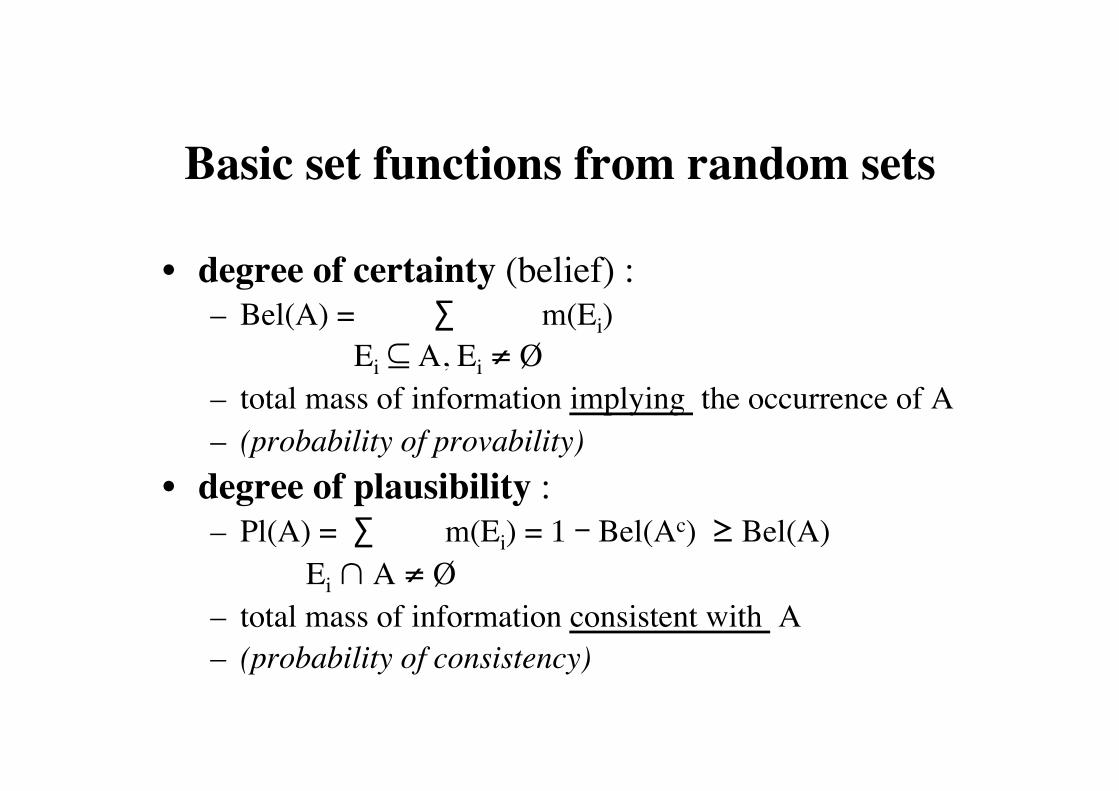
Basic set functions from random sets
• degree of certainty (belief) : – Bel(A) = ∑ m(Ei) Ei ⊆ A, Ei ≠ Ø
– total mass of information implying the occurrence of A – (probability of provability)
• degree of plausibility : – Pl(A) = ∑ m(Ei) = 1 - Bel(Ac) ≥ Bel(A) Ei ∩ A ≠ Ø
– total mass of information consistent with A – (probability of consistency)
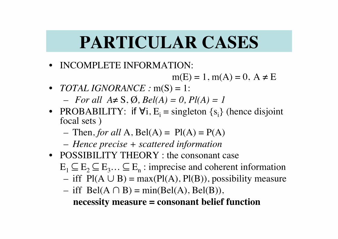
PARTICULAR CASES • INCOMPLETE INFORMATION: m(E) = 1, m(A) = 0‚ A ≠ E • TOTAL IGNORANCE : m(S) = 1:
– For all A≠ S, Ø, Bel(A) = 0, Pl(A) = 1 • PROBABILITY: if ∀i, Ei = singleton si (hence disjoint
focal sets ) – Then, for all A, Bel(A) = Pl(A) = P(A) – Hence precise + scattered information
• POSSIBILITY THEORY : the consonant case E1 ⊆ E2 ⊆ E3… ⊆ En : imprecise and coherent information
– iff Pl(A ∪ B) = max(Pl(A), Pl(B)), possibility measure – iff Bel(A ∩ B) = min(Bel(A), Bel(B)), necessity measure = consonant belief function
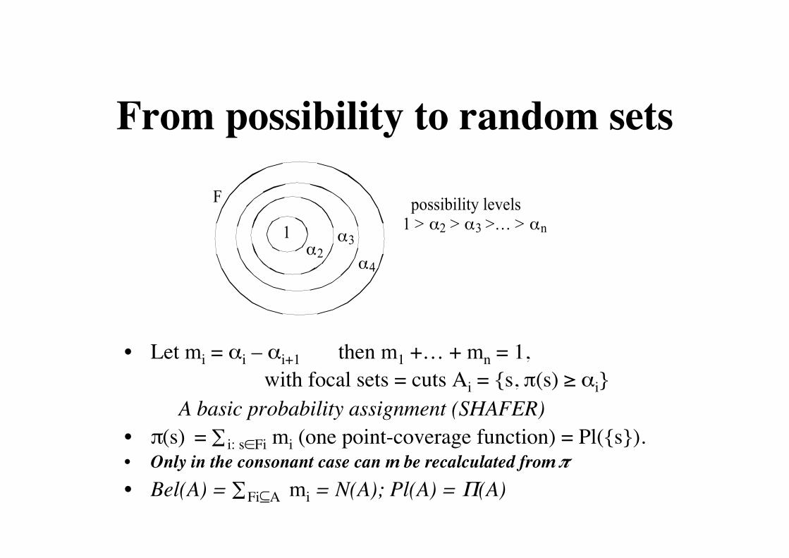
From possibility to random sets
• Let mi = αi – αi+1 then m1 +… + mn = 1, with focal sets = cuts Ai = s, π(s) ≥ αi
A basic probability assignment (SHAFER) • π(s) = ∑i: s∈Fi mi (one point-coverage function) = Pl(s). • Only in the consonant case can m be recalculated from π • Bel(A) = ∑Fi⊆A mi = N(A); Pl(A) = Π(A)
1
F
!3
possibility levels1 > !2 > !3 >… > !n
!2!4
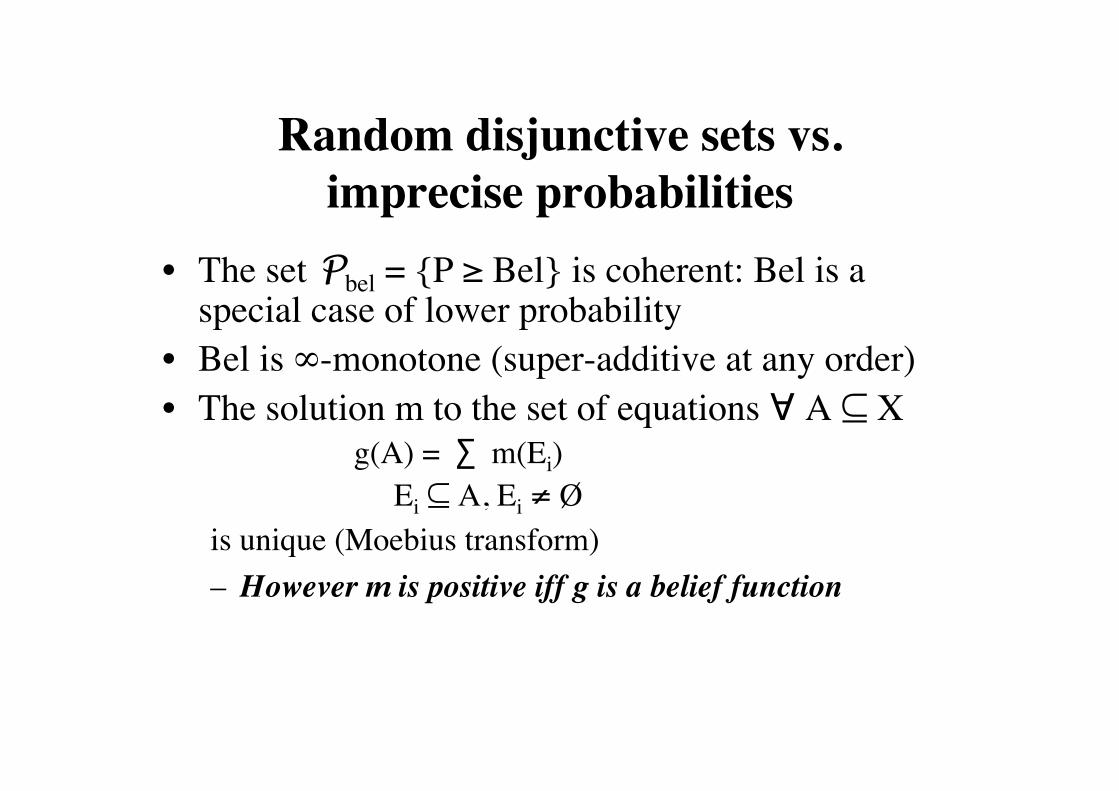
Random disjunctive sets vs. imprecise probabilities
• The set Pbel = P ≥ Bel is coherent: Bel is a special case of lower probability
• Bel is ∞-monotone (super-additive at any order) • The solution m to the set of equations ∀ A ⊆ X
g(A) = ∑ m(Ei) Ei ⊆ A, Ei ≠ Ø
is unique (Moebius transform) – However m is positive iff g is a belief function

Dempster original model
• Indirect information (induced from a probability space).
• What we know about a random variable x with range S, based on a sample space (Ω, A, P) and a multimapping Γ from Ω to S (Dempster):
• The meaning of the multimapping Γ from Ω to S : – if we observe ω in Ω then all we know is x (ω) ∈ Γ(ω)
• m(Γ(ω)) = P(ω) ∀ ω in Ω (finite case.) • Then a belief function is a lower probability.

Dempster vs. Shafer-Smets • A disjunctive random set can represent
– Uncertain singular evidence (unreliable testimonies): m(E) = subjective probability pertaining to the truth of testimony E.
• Degrees of belief directly modelled by Bel : no appeal to an underlying probability.
(Shafer, 1976 book; Smets) – Imprecise statistical evidence: m(E) = frequency of imprecise
observations of the form E and Bel(E) is a lower probability • A multiple-valued mapping from a probability space to a space of
interest representing an ill-known random variable. • Here, belief functions are explicitly viewed as lower probabilities
(Dempster intuition) • In all cases E is a set of mutually exclusive values and does
not represent a real set-valued entity

Canonical examples
• Statistical probabilities : Frequentist modelling of a collection of incomplete observations (imprecise statistics) : incomplete generic information
• Uncertain singular information: – Unreliable testimonies (Shafer’s book) : unreliable singular information
– Unreliable sensors : the quality of the information depends on the ill-known sensor state.

Example of uncertain evidence : Unreliable testimony (SHAFER-SMETS VIEW)
• « John tells me the president is between 60 and 70 years old, but there is some chance (subjective probability p) he does not know and makes it up». – E =[60, 70]; Prob(Knowing “x∈ E =[60, 70]”) = 1 - p. – With probability p, John invents the info, so we know nothing (Note
that this is different from a lie). • We get a simple support belief function : m(E) = 1 – p and m(S) = p
• Equivalent to a possibility distribution – π(s) = 1 if x ∈ E and π(s) = p otherwise.
• If John may lie (probability q): m(E) = (1 – p)(1 – q), m(Ec) = (1 – p)q.

Example of generic belief function: imprecise observations in an opinion poll
• Question : who is your preferred candidate in C = a, b, c, d, e, f ???
– To a population Ω = 1, …, i, …, n of n persons. – Imprecise responses r = « x(i) ∈ Ei » are allowed – No opinion (r =C) ; « left wing » r = a, b, c ; – « right wing » r = d, e, f ; – a moderate candidate : r = c, d
• Definition of mass function: – m(E) = card(i, Ei = E)/n – = Proportion of imprecise responses « x(i) ∈ E »

• The probability that a candidate in subset A ⊆ C is elected is imprecise :
Bel(A) ≤ P(A) ≤ Pl(A) • There is a fuzzy set F of potential winners:
µF(x) = ∑ x ∈ E m(E) = Pl(x) (contour function) • µF(x) is an upper bound of the probability that x is elected.
It gathers responses of those who did not give up voting for x
• Bel(x) gathers responses of those who claim they will vote for x and no one else.

Example of conjunctive random sets Experiment on linguistic capabilities of people : • Question to a population Ω = 1, …, i, …, n of n
persons: which languages can you speak ? • Answers : Subsets in L = Basque, Chinese, Dutch,
English, French,…. ? • m(E) = % people who speak exactly all languages in E
(and not other ones) • Prob(x speaks A) =∑m(E) : A⊆E = Q(A) : commonality
function in belief function theory • Example: « x speaks English » means « at least English » • The belief function is not meaningful here while the
commonality makes sense, contrary to the disjunctive set case.

POSSIBILITY AS UPPER PROBABILITY
• Given a numerical possibility distribution π, define P(π) = P | P(A) ≤ Π(A) for all A
– Then, Π and N can be recovered • Π(A) = sup P(A) | P ∈ P(π); • N(A) = inf P(A) | P ∈ P(π)
– So π is a faithful representation of a special family of probability measures
• Likewise for belief functions : P(m) = P | P(A) ≤ Pl(A), ∀ A • Pl(A) = sup P(A) | P ∈ P(m); • Bel(A) = inf P(A) | P ∈ P(m)
• But this view makes sense for belief functions – Representing statistical knowledge – Representing maximal buying prices as per Walley

LIKELIHOOD FUNCTIONS
• Likelihood functions λ(x) = P(A| x) behave like possibility distributions when there is no prior on x, and λ(x) is used as the likekihood of x.
• It holds that λ(B) = P(A| B) ≤ maxx ∈ B P(A| x) • If P(A| B) = λ(B) then λ should be set-monotonic: x ⊆ B implies λ(x) ≤ λ(B)
It implies λ(B) = maxx ∈ B λ(x)
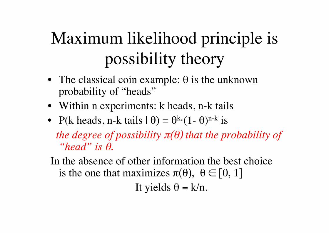
Maximum likelihood principle is possibility theory
• The classical coin example: θ is the unknown probability of “heads”
• Within n experiments: k heads, n-k tails • P(k heads, n-k tails | θ) = θk·(1- θ)n-k is the degree of possibility π(θ) that the probability of
“head” is θ. In the absence of other information the best choice
is the one that maximizes π(θ), θ ∈ [0, 1] It yields θ = k/n.

LANDSCAPE OF UNCERTAINTY THEORIES BAYESIAN/STATISTICAL PROBABILITY: the language of unique probability distributions (Randomized points) UPPER-LOWER PROBABILITIES : the language of disjunctive convex sets of probabilities, and lower expectations
SHAFER-SMETS BELIEF FUNCTIONS: The language of Moebius masses (Random disjunctive sets) QUANTITATIVE POSSIBILITY THEORY : The language of possibility distributions (Fuzzy (nested disjunctive) sets) BOOLEAN POSSIBILITY THEORY (modal logic KD45) : The language of Disjunctive sets

Practical representation issues
• Lower probabilities are difficult to represent (2|S| values): The corresponding family is a polyhedron with potentially |S|! vertices.
• Finite random sets are simpler but potentially 2|S| values
• Possibility measures are simple (|S| values) but sometimes not expressive enough.
• There is a need for simple and more expressive representations of imprecise probabilities or random sets.
Practical representations
• Fuzzy intervals (continuous consonant bf) • Probability intervals • Probability boxes (continuous random
intervals with comonotonic bounds) • Generalized p-boxes • Clouds Some are special random sets some not.

From confidence sets to possibility distributions
• Let E1, E2, …En be a nested family of sets • A set of confidence levels a1, a2, …an in [0, 1] • Consider the set of probabilities
P = P, P(Ei) ≥ ai, for i = 1, …n • Then P is representable by means of a possibility
measure with distribution π(x) = mini = 1, …n max (µEi(x), 1- ai)

a1
a2
1
0
E1
E2
E3
π
POSSIBILITY DISTRIBUTION INDUCED BY EXPERT CONFIDENCE INTERVALS
α2
α3
m2= α2 - α3
1
0
π
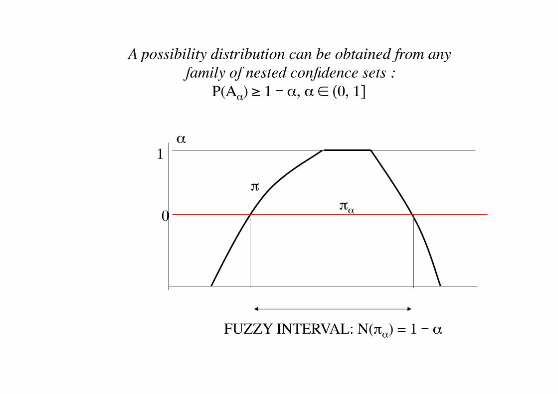
α
πα
FUZZY INTERVAL: N(πα) = 1 - α
A possibility distribution can be obtained from any family of nested confidence sets :
P(Αα) ≥ 1 - α, α ∈ (0, 1]

Possibilistic view of probabilistic inequalities
• Probabilistic inequalities can be used for knowledge representation – Chebyshev inequality defines a possibility distribution that dominates
any density with given mean and variance:
P(V ∈ [xmean – kσ, xmean + kσ]) ≥ 1 – 1/k2 is equivalent to writing π(xmean – kσ) = π(xmean + kσ) = 1/k2 – A triangular fuzzy number (TFN) defines a possibility distribution that
dominates any unimodal density with the same mode and bounded support as the TFN.

Optimal order-faithful fuzzy prediction interval

Chebychev Camp-Meidel
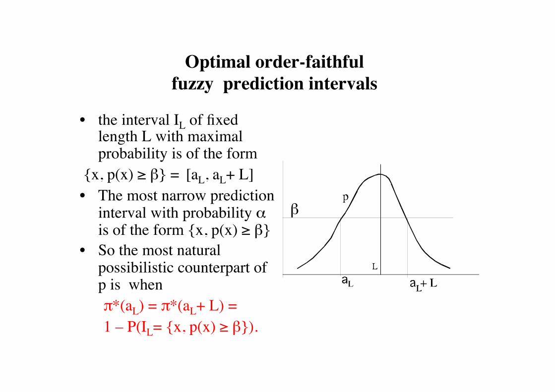
• the interval IL of fixed length L with maximal probability is of the form
x, p(x) ≥ β = [aL, aL+ L] • The most narrow prediction
interval with probability α is of the form x, p(x) ≥ β
• So the most natural possibilistic counterpart of p is when
π*(aL) = π*(aL+ L) = 1 – P(IL= x, p(x) ≥ β).
Optimal order-faithful fuzzy prediction intervals
β

Probability boxes • A set P = P: F* ≥ P ≥ F* induced by two
cumulative disribution functions is called a probability box (p-box),
• A p-box is a special random interval (continuous belief function) whose upper and bounds induce the same ordering.
• A fuzzy interval induces a p-box P
F*
F*
0
1
α
Eα

Probability boxes from possibility distributions
• Representing families of probabilities by fuzzy intervals is more precise than with the corresponding pairs of PDFs:
– F*(a) = ΠM( ( -∞, a]) = M(a) if a ≤ m = 1 otherwise.
– F*(a) = NM( ( -∞, a] ) = 0 if a < m*
= 1 - limx ↓ aM(x) otherwise • P(π) is a proper subset of P
– Not all P in P: F* ≥ P ≥ F* are such that Π ≥ P

P-boxes vs. fuzzy intervals
0 1 2 3 0
1
0.5 F* F* π
A triangular fuzzy number with support [1, 3] and mode 2. Let P be defined by P(1.5)=P(2.5)=0.5. Then F* < F < F P ∉ P(Π) since P(1.5, 2.5) = 1 > Π(1.5, 2.5) = 0.5

Generalized cumulative distributions
• A Cumulative distribution function F of a probability function P can be viewed as a possibility distribution dominating P supF(x), x ∈ A ≥ P(A)
• Choosing any order relation ≤R FR(x) = P(y ≤R x) also induces a possibility distribution dominating P
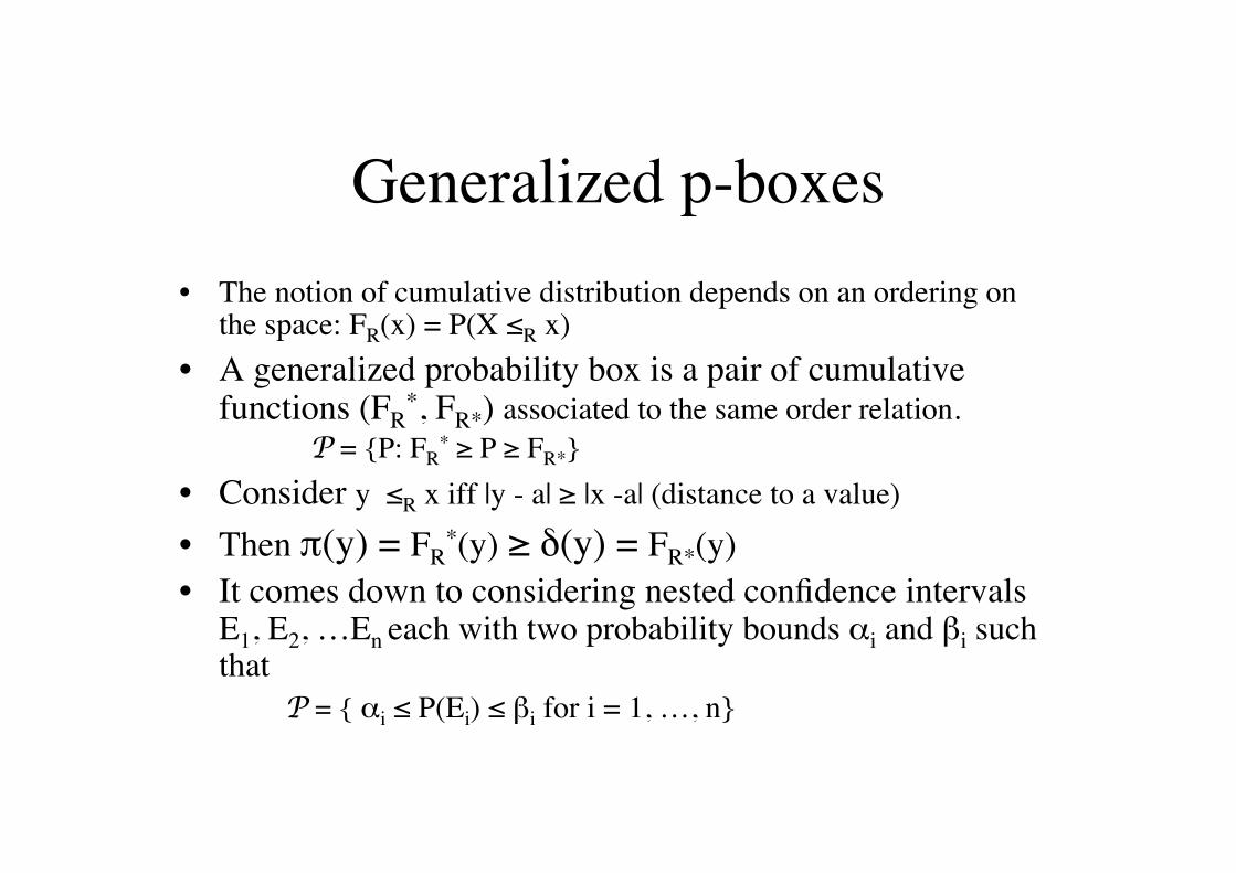
Generalized p-boxes • The notion of cumulative distribution depends on an ordering on
the space: FR(x) = P(X ≤R x) • A generalized probability box is a pair of cumulative
functions (FR*, FR*) associated to the same order relation.
P = P: FR* ≥ P ≥ FR*
• Consider y ≤R x iff |y - a| ≥ |x -a| (distance to a value)
• Then π(y) = FR*(y) ≥ δ(y) = FR*(y)
• It comes down to considering nested confidence intervals E1, E2, …En each with two probability bounds αi and βi such that P = αi ≤ P(Ei) ≤ βi for i = 1, …, n

Generalized p-boxes • It comes down to two possibility distributions π (from αi ≤ P(Ei)) and πc (from P(Ei) ≤ βi ) • Distributions π and πc are such that π ≥ 1 - πc = δ and π is comonotonic with δ (they induce the same order on the referential according to ≤R).
• P = P (π) ∩ P (πc) • Theorem: a generalized p-box is a belief function
(random set) with focal sets x: π(x) ≥ α \ x: δ(x) > α

From generalized p-boxes to clouds

CLOUDS
• Neumaier (2004) proposed a generalized interval as a pair of distributions (π ≥ δ) on a referential representing the family of probabilities P = P, s. t. P(x: δ(x) > α) ≤ α ≤ P(x: π(x) ≥ α) ∀α >0
• Distributions π and 1- δ are possibility distributions such that P = P (π) ∩ P (1-δ)
• It does not correspond to a belief function, not even a convex (2-monotone) capacity

SPECIAL CLOUDS • Clouds are modelled by interval-valued fuzzy sets • Comonotonic clouds = generalized p-boxes • Fuzzy clouds: δ = 0; they are possibility distributions
• Thin clouds: π = δ: – Finite case : empty – Continuous case : there is an infinity of probability
distributions in P (π) ∩ P (1-π) for bell-shaped π – Increasing π: only one probability measure p (π =
cumulative distribution of p)

Probability intervals • Probability intervals = a finite collection L of imprecise
assignments [li , ui ] attached to elements si of a finite set S. • A collection L = [li , ui ] i = 1,… n induces the family PL
= P: li ≤ P(si) ≤ ui. • Lower/upper probabilities on events are given by
– P*(A) = max(Σsi∈A li ; 1 – Σsi∉A ui) ; – P*(A) = min(Σsi∈A ui ; 1 – Σsi∉A li)
• P* is a 2-monotone Choquet capacity

How useful are these representations:
• P-boxes can address questions about threshold violations (x ≥ a ??), not questions of the form a ≤ x≤ b
• The latter questions are better addressed by possibility distributions or generalized p-boxes

Relationships between representations
• Generalized p-boxes are special random sets that generalize BOTH p-boxes and possibility distributions
• Clouds extend GP-boxes but induce lower probabilities that are not even 2-monotonic.
• Probability intervals are not comparable to generalized p-boxes: they induce lower probabilities that are 2-monotonic

Important pending theoretical issues
• Comparing representations in terms of informativeness.
• Conditioning : several definitions for several purposes.
• Independence notions: distinguish between epistemic and objective notions.
• Find a general setting for information fusion operations (e.g. Dempster rule of combination).

Comparing belief functions in terms of informativeness
• Consonant case : relative specificity. π' more specific (more informative) than π in
the wide sense if and only if π' ≤ π. (any possible value in information state π' is
at least as possible in information state π) – Complete knowledge: π(s0) = 1 and = 0
otherwise. – Ignorance: π(s) = 1, ∀ s ∈ S

Comparing belief functions in terms of informativeness
• Using contour functions: π(s)= Pl(s) = ∑x ∈ E m(E)
m1 is more cf-informative that m2 iff π1 ≤ π2
• Using belief or plausibility functions : m1 is more pl-informative that m2 iff Pl1 ≤ Pl2
iff Bel1 ≥ Bel2 It corresponds to comparing credal sets P(m): Pl1 ≤ Pl2 if and only if P(m1) ⊆ P(m2)
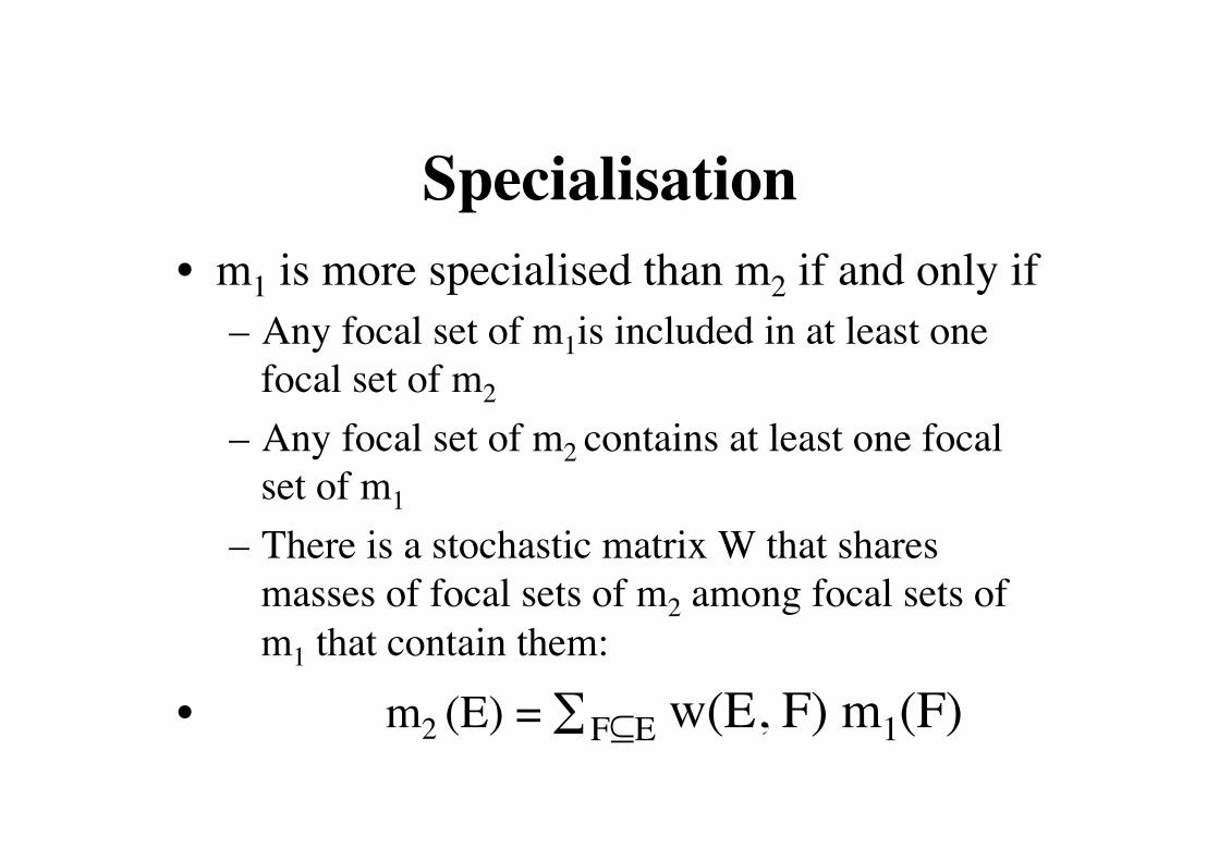
Specialisation • m1 is more specialised than m2 if and only if
– Any focal set of m1is included in at least one focal set of m2
– Any focal set of m2 contains at least one focal set of m1
– There is a stochastic matrix W that shares masses of focal sets of m2 among focal sets of m1 that contain them:
• m2 (E) = ∑F⊆E w(E, F) m1(F)
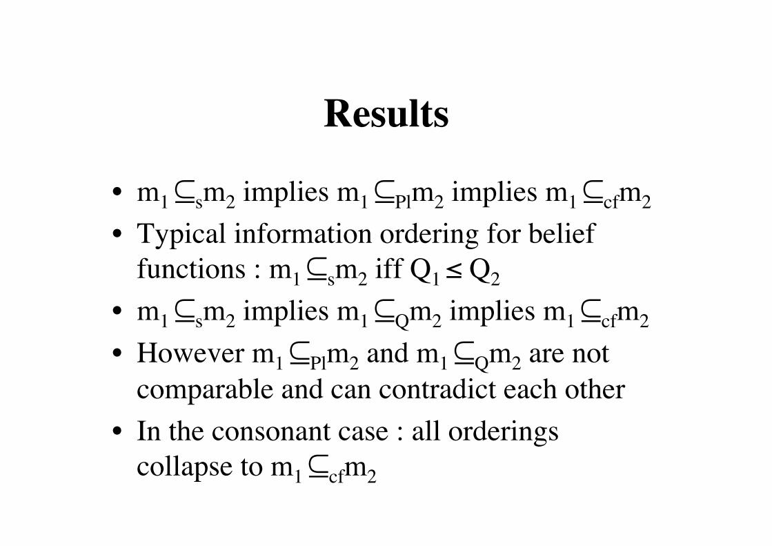
Results
• m1 ⊆sm2 implies m1 ⊆Plm2 implies m1 ⊆cfm2
• Typical information ordering for belief functions : m1 ⊆sm2 iff Q1 ≤ Q2
• m1 ⊆sm2 implies m1 ⊆Qm2 implies m1 ⊆cfm2
• However m1 ⊆Plm2 and m1 ⊆Qm2 are not comparable and can contradict each other
• In the consonant case : all orderings collapse to m1 ⊆cfm2

Example
• S = a, b, c; m1(ab) = 0.5, m1(bc) = 0.5; • m2(abc) = 0.5, m2(b) = 0.5 • m1 ⊆sm2 nor m2 ⊆sm1 hold • m2 ⊂Plm1 : Pl1(A) = Pl2(A)
but Pl2(ac) = 0.5 < Pl1(ac) = 1 • m1 ⊂Qm2 : Q1(A) = Q2(A)
but Q1(ac) = 0 < Q2(ac) = 0.5 • And contour functions are equal : a/0.5, b/1, c/0.5

Conditional probability
• Querying a generic probability based on sure singular information: – P represents generic information (statistics over
a population), – C represents singular evidence (variable
instantiation for a case x at hand) – The relative frequency P(B|C) is used as the
degree of belief that x∈C satisfies B.

Conditional probability
• Revising a subjective probability – P(A) represents singular information, an
agent’s prior belief on what is the current state of the world (that a birth date x∈A…).
– C represents an additional sure information about the value of x : x∈C for sure.
– P(A|C) represents the agent’s posterior belief that x∈A.
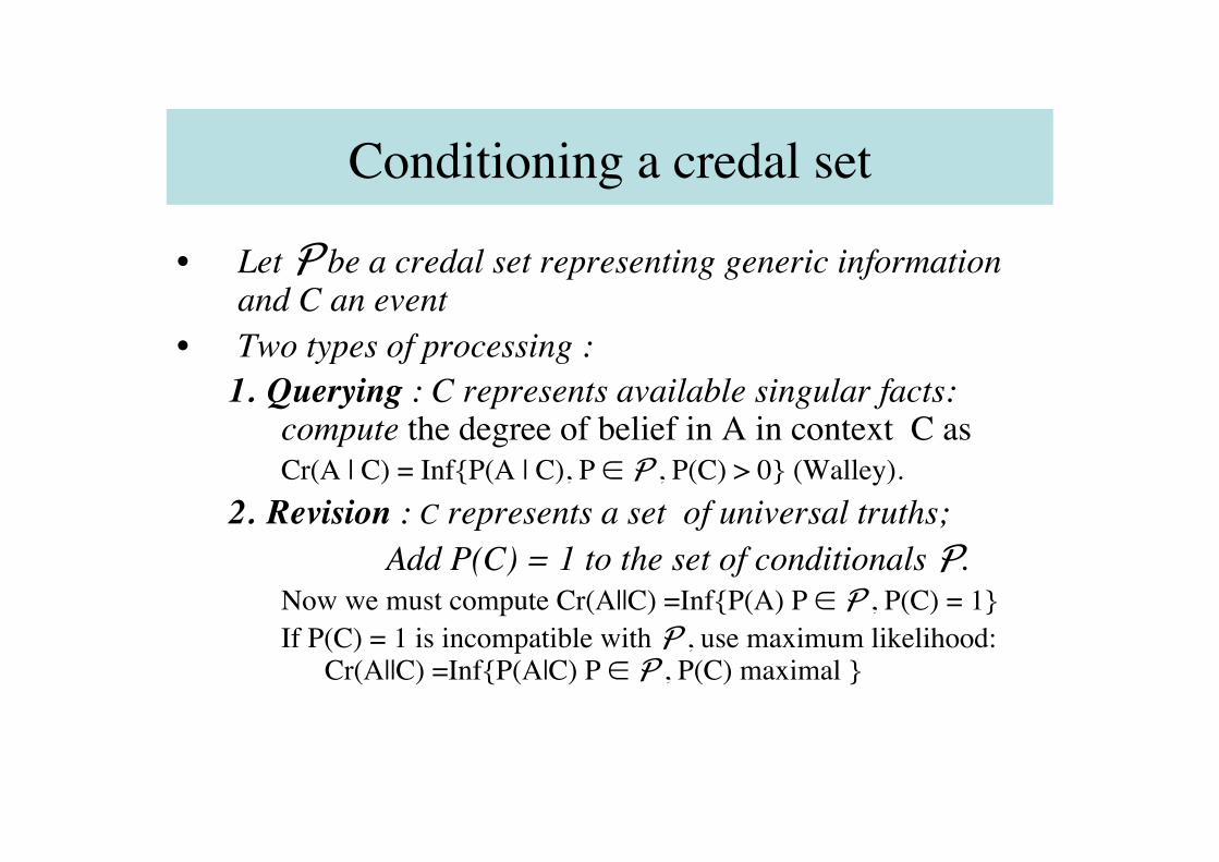
Conditioning a credal set • Let P be a credal set representing generic information
and C an event • Two types of processing :
1. Querying : C represents available singular facts: compute the degree of belief in A in context C as Cr(A | C) = InfP(A | C), P ∈ P , P(C) > 0 (Walley).
2. Revision : C represents a set of universal truths; Add P(C) = 1 to the set of conditionals P. Now we must compute Cr(A||C) =InfP(A) P ∈ P , P(C) = 1 If P(C) = 1 is incompatible with P , use maximum likelihood:
Cr(A||C) =InfP(A|C) P ∈ P , P(C) maximal

Example : A B C • P is the set of probabilities such that
– P(B|A) ≥ α Most A are B – P(C|B) ≥ β Most B are C – P(A|B) ≥ γ Most B are A
• Querying on context A : Find the most narrow interval for P(C|A) (Linear programming): we find
P(C|A) ≥ α ⋅ max(0, 1 - (1 - β)/γ) – Note : if γ = 0 , P(C|A) is unknown even if α = 1.
• Revision: Suppose P(A) = 1, then P(C||A) ≥ α⋅β – Note: β > max(0, 1 - (1 - β)/γ)
• Revision improves generic knowledge, querying does not.

CONDITIONING RANDOM SETS AS IMPRECISE PROBABILISTIC INFORMATION
• A disjunctive random set (F, m) representing background knowledge is equivalent to a set of probabilities P = P: ∀A, P(A) ≥ Bel(A) (NOT conversely).
• Querying this information based on evidence C comes down to performing a sensitivity analysis on the conditional probability P(·|C) – BelC(A) = inf P(A|C): P ∈ P, P(C) >0 – PlC(A) = sup P(A|C): P ∈ P, P(C) >0
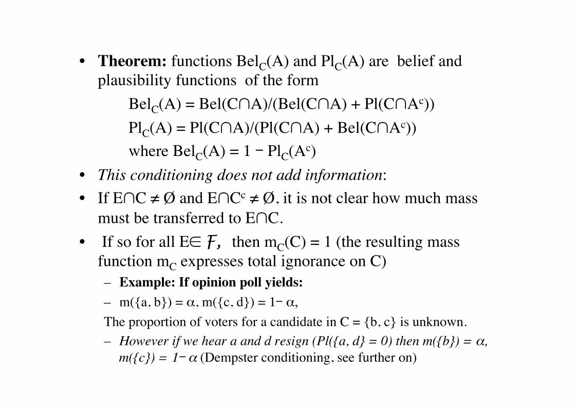
• Theorem: functions BelC(A) and PlC(A) are belief and plausibility functions of the form BelC(A) = Bel(C∩A)/(Bel(C∩A) + Pl(C∩Ac)) PlC(A) = Pl(C∩A)/(Pl(C∩A) + Bel(C∩Ac)) where BelC(A) = 1 - PlC(Ac)
• This conditioning does not add information: • If E∩C ≠ Ø and E∩Cc ≠ Ø, it is not clear how much mass
must be transferred to E∩C. • If so for all E∈ F, then mC(C) = 1 (the resulting mass
function mC expresses total ignorance on C) – Example: If opinion poll yields: – m(a, b) = α, m(c, d) = 1- α,
The proportion of voters for a candidate in C = b, c is unknown. – However if we hear a and d resign (Pl(a, d = 0) then m(b) = α,
m(c) = 1- α (Dempster conditioning, see further on)

CONDITIONING UNCERTAIN SINGULAR EVIDENCE
• A mass function m on S, represents uncertain evidence • A new sure piece of evidence is viewed as a conditioning
event C 1. Mass transfer : for all E ∈ F, m(E) moves to C ∩ E ⊆ C
– The mass function after the transfer is mt(B) = Σ E : C ∩ E = B m(E) – But the mass transferred to the empty set may not be zero! – mt(∅) = Bel(Cc) = Σ E : C ∩ E = Ø m(E) is the degree of conflict
with evidence C 3. Normalisation: mt(B) should be divided by
Pl(C) = 1 - Bel(Cc) = Σ E : C ∩ E ≠ Ø m(E) • This is revision of an unreliable testimony by a sure fact

DEMPSTER RULE OF CONDITIONING = PRIORITIZED MERGING
The conditional plausibility function Pl(.|C) is Pl(A ∩ C) Pl(A||C) = ; Bel(A||C) = 1- Pl(Ac||C) Pl(C)
• C surely contains the value of the unknown quantity described by m. So Pl(Cc) = 0 – The new information is interpreted as asserting the
impossibility of Cc: Since Cc is impossible you can change x ∈ Ε into x ∈ E∩ C and transfer the mass of focal set E to E ∩ C.
• The new information improves the precision of the evidence : This conditioning is different from Bayesian (Walley) conditioning

EXAMPLE OF REVISION OF EVIDENCE : The criminal case
• Evidence 1 : three suspects : Peter Paul Mary • Evidence 2 : The killer was randomly selected
man vs.woman by coin tossing. – So, S = Peter, Paul, Mary
• TBM modeling: The masses are m(Peter, Paul) = 1/2 ; m(Mary) = 1/2 – Bel(Paul) = Bel(Peter) = 0. Pl(Paul) = Pl(Peter) = 1/2 – Bel(Mary) = Pl(Mary) = 1/2
• Bayesian Modeling: A prior probability – P(Paul) = P(Peter) = 1/4; P(Mary) = 1/2

• Evidence 3 : Peter was seen elsewhere at the time of the killing. • TBM: So Pl(Peter) = 0.
– m(Peter, Paul) = 1/2; mt(Paul) = 1/2 – A uniform probability on Paul, Mary results.
• Bayesian Modeling: – P(Paul | not Peter) = 1/3; P(Mary | not Peter) = 2/3. – A very debatable result that depends on where the story starts.
Starting with i males and j females: • P(Paul | Paul OR Mary) = j/(i + j); • P(Mary | Paul OR Mary) = i/(i + j)
• Walley conditioning: – Bel(Paul) = 0; Pl(Paul) = 1/2 – Bel(Mary) = 1/2; Pl(Mary) = 1

Information fusion • Dempster rule of combination in evidence theory:
– independent sources, normalised or not – Does nor preserve consonance of inputs – No well-accepted idempotent fusion rule.
• In possibility theory : many fusion rules. – The minimum rule : idempotent (= minimal
commitment fusion rule for consonant belief functions, not for other ones)
– The product rule : coincides with the contour function obtained from unnormalized Dempster rule applied to consonant belief functions
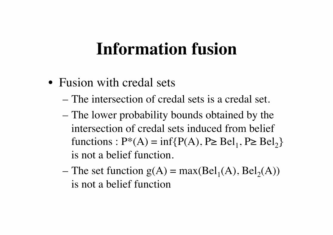
Information fusion
• Fusion with credal sets – The intersection of credal sets is a credal set. – The lower probability bounds obtained by the
intersection of credal sets induced from belief functions : P*(A) = infP(A), P≥ Bel1, P≥ Bel2 is not a belief function.
– The set function g(A) = max(Bel1(A), Bel2(A)) is not a belief function

Decision with imprecise probability techniques
• Accept incomparability when comparing imprecise utility evaluations of decisions. – Pareto optimality : decisions that dominate other choices for all
probability functions – E-admissibility : decisions that dominate other choices for at least
one probability function (Walley, etc…) • Select a single utility value that achieves a compromise
between pessimistic and optimistic attitudes. – Select a single probability measure (Shapley value = pignistic
transformation) and use expected utility (SMETS) – Compare lower expectations of decisions (Gilboa) – Generalize Hurwicz criterion to focal sets with degree of optimism
(Jaffray)

Conclusion • There exist a coherent range of uncertainty theories
combining interval and probability representations. – Imprecise probability is the proper theoretical umbrella – The choice between subtheories depends on how expressive
it is necessary to be in a given application. – There exists simple practical representations of imprecise
probability : possibility theory is the simplest, and belief functions are a good compromise between calculability and expressivity
• Discrepancies between the theories remain on conditioning, combination rules, because their language primitives differ: – One cannot obviously express concepts defined by
probability masses using credal sets, and conversely, let alone possibility distributions.