energies

Article

Development of a General Package for Resolution ofUncertainty-Related Issues in Reservoir Engineering

Liang Xue 1,2, Cheng Dai 3,* and Lei Wang 4

1 Department of Oil-Gas Field Development Engineering, College of Petroleum Engineering,China University of Petroleum, Beijing 102249, China; xueliang@pku.edu.cn

2 State Key Laboratory of Petroleum Resources and Prospecting, China University of Petroleum,Beijing 102249, China

3 State Key Laboratory of Shale Oil and Gas Enrichment Mechanisms and Effective Development,SINOPEC Group, Beijing 050021, China

4 Department of Energy and Resources Engineering, College of Engineering, Peking University,Beijing 100871, China; wanglei1986sp@foxmail.com

* Correspondence: daicheng@pku.edu.cn; Tel.: +86-10-8231-2089

Academic Editor: Mofazzal HossainReceived: 20 November 2016; Accepted: 2 February 2017; Published: 10 February 2017

Abstract: Reservoir simulations always involve a large number of parameters to characterize theproperties of formation and fluid, many of which are subject to uncertainties owing to spatialheterogeneity and insufficient measurements. To provide solutions to uncertainty-related issues inreservoir simulations, a general package called GenPack has been developed. GenPack includesthree main functions required for full stochastic analysis in petroleum engineering, generation ofrandom parameter fields, predictive uncertainty quantifications and automatic history matching.GenPack, which was developed in a modularized manner, is a non-intrusive package which canbe integrated with any existing commercial simulator in petroleum engineering to facilitate itsapplication. Computational efficiency can be improved both theoretically by introducing a surrogatemodel-based probabilistic collocation method, and technically by using parallel computing. A seriesof synthetic cases are designed to demonstrate the capability of GenPack. The test results show that therandom parameter field can be flexibly generated in a customized manner for petroleum engineeringapplications. The predictive uncertainty can be reasonably quantified and the computational efficiencyis significantly improved. The ensemble Kalman filter (EnKF)-based automatic history matchingmethod can improve predictive accuracy and reduce the corresponding predictive uncertainty byaccounting for observations.

Keywords: reservoir simulation; uncertainty quantification; automatic history matching

1. Introduction

With the advancement of the quantitative modeling techniques in petroleum engineering,numerical simulations have become popular for describing subsurface flow characteristics andmaking predictions with respect to subsurface flow behaviors. Common numerical simulators, suchas Schlumberger Eclipse, CMG and TOUGH2, are widely used in petroleum engineering to aiddecision-making for oil extraction. The most severe challenge posed by the need to obtain accuratepredictions of oil production in a reservoir lies in the various sources of uncertainties associatedwith a selected predictive model. The uncertainties may stem from the spatial heterogeneity of theformation properties caused by the complex geological process and insufficient measurements limitedby technological and economic factors. The uncertainty-related issues appear in two essential processesrequired by a complete reservoir modeling project: forward modeling and inverse modeling.

Energies 2017, 10, 197; doi:10.3390/en10020197 www.mdpi.com/journal/energies

Energies 2017, 10, 197 2 of 16

The uncertainty-related issue in forward modeling processes is related to quantification of theprediction uncertainties and risks for a given numerical model with several uncertain parameters [1–3].Monte Carlo simulation (MCS) is the most widely used uncertainty quantification method. It hasbeen applied to petroleum engineering and groundwater hydrology [4–8]. MCS requires generating alarge number of realizations of the random inputs in order to obtain a reasonably converged result [1],which is achieved with a high computational cost. This cost may become unaffordable in some cases,especially when each simulation is already time-consuming. In recent years, a surrogate model-basedmethod, called probabilistic collocation method (PCM), has been developed by some researchers [3,9].The PCM method consists of two parts, the representation of the random variables using polynomialchaos basis and the derivation of the appropriate discretized equations for the expansion coefficientson selected collocation points. This method was applied to the fields of petroleum engineering andgroundwater hydrology [10,11] to estimate predictive risks.

Inverse modeling, also known as data assimilation or history matching, aims to reduce thepredictive uncertainty through model calibration assisted by the production data. Traditional inversemodeling process is implemented by hand so that the simulation output can match the production datawell, and the performance of the calibration results strongly depends on engineer experience. However,this traditional inverse modeling method is inefficient and sometimes infeasible for application incomplex models with a large number of parameters. Many automatic history matching methodshave been developed recently [12–15]. Attributing to the development of the in-situ monitoringtechniques, a sequential stochastic inversing modeling method, the ensemble Kalman filter (EnKF),attracts a lot of attention. Apart from its conceptual simplicity and easy implementation, the followingfactors support the popularity of the EnKF method: (a) it is a non-intrusive method, which can beintegrated in a straightforward manner with already available simulators; (b) it allows the flexibility toprovide the uncertainty associated with the system states at each assimilation step; and (c) it can beextended to enable us to handle a large number of parameters to characterize subsurface flow systemsunder uncertainty [16–21]. The EnKF procedure is composed of two stages: the forecast stage and theassimilated stage. The field is first parameterized and represented by a set of realizations in terms ofprior knowledge. In the forecast stage, the model response of each realization is propagated forwardin time. In the assimilated stage, the parameters of each realization are updated by assimilatingavailable observations [16]. The successful use of EnKF in various areas has been reported in manyliteratures [22–25].

Since uncertainty-related issues are ubiquitous in petroleum engineering, there is an urgentneed to develop a software package that has the capability to integrate various state-of-the-artstochastic forward and inverse modeling methods and conduct a complete stochastic analysis toaid the decision-making for a given project. Here, we develop a general package, named GenPack,to handle a comprehensive set of the uncertainty-related issues. To our knowledge, no similarsoftware package has been developed in the petroleum engineering field. The innovations of ourdeveloped GenPack are that: (a) it is programmed in a modularized manner and can be extendedeasily when new functions are required; (b) it is customized to petroleum engineering applicationsand is ready to be integrated with any existing simulator, thus it can be easily implemented bypetroleum engineers; (c) theoretical analysis methods, such as probabilistic collocation method andparallel computing techniques, are both used to tackle the obstacles regarding computational efficiencyin stochastic analysis. The purpose of GenPack is to facilitate the implementation of stochasticanalysis required by either researchers or engineers, and it also provides a platform to easily integratewith other functions when new methods are created. This package is freely available upon request(https://www.researchgate.net/publication/313114201_GenPack_Code).

This paper is organized as follows. Section 2 illustrates the theoretical bases required in thedeveloped general software package. Section 3 is devoted to demonstrating the capability of thepackage to quantify uncertainty and implement automatic history matching. Conclusions are presentedin Section 4.

Energies 2017, 10, 197 3 of 16

2. Methodology

The developed GenPack software includes three main features. These features are the generationof the random parameter field, the stochastic forwarding modeling to quantify the predictiveuncertainty, and automatic history matching to calibrate the numerical model against the sequentiallyavailable data. The methods selected to achieve the desired features are either widely accepted(e.g., sequential Gaussian simulation method and the ensemble Kalman filter method) or performedwell based on our research experiences (e.g., the Karhunen–Loeve expansion method and probabilisticcollocation method). In this section, the theoretical bases of all these built-in methods are introduced.

2.1. Random Field Generator

To characterize the heterogeneity of geological parameters, such as permeability and porosity,it is common to treat these parameters as Gaussian random fields. GenPack provides two options togenerate the Gaussian random field, sequential Gaussian simulation method and Karhunen–Loeve(KL) expansion.

2.1.1. Sequential Gaussian Simulation Method

Gaussian sequential simulation method [1] is based on conditional probability densityfunction (PDF),

p(k1, k2, . . . , kn) = p(k1, k2, . . . , kn−1)p(kn|k1, k2, . . . , kn−1)

= . . .= p(k1)p(k2|k1) . . . p(kn|k1, k2, . . . , kn−1)

(1)

where kn denotes the parameter value at the location xn, i.e., kn = k(xn).According to the first part of Equation (1), an n-dimensional joint PDF of p(k1, k2, . . . , kn) can be

expressed by the product of an (n − 1)-dimensional conditional PDF and an unconditional PDF. If wekeep re-iterating this process, we can obtain the final form of Equation (1). This equation indicatesthat we can generate a trajectory of (n − 1) parameter values, i.e., k2, . . . , kn by taking advantage ofthe successive form of the conditional probability relation, once the first one is randomly drawn fromthe unconditional Gaussian PDF p(k1) with the known mean and variance of the field. The mean andvariance of the conditional PDF following a Gaussian distribution can be determined by:

〈k(xn)〉c = 〈k(xn)〉+n−1

∑i=1

ai(xn)[ki − 〈k(xi)〉] (2)

Varc[k(xn)] = σ2k (xn)−

n−1

∑i=1

ai(xn)Ck(xi − xn) (3)

where superscript c stands for conditional, and σ2k(xn) and Ck

(xi − xj

)are variance and covariance of

geological parameter k(xn), respectively.The coefficients {ai(xn)} can be solved using the following equation:

n−1

∑j=1

aj(xn)Ck(

xi − xj)= Ck(xi − xn), i = 1, . . . , n− 1 (4)

2.1.2. Karhunen–Loeve Expansion

KL expansion [10] is an alternative method to generate a random field. Let k(x, θ) be a randomspace function, where x ∈ D and θ ∈ Θ (a probability space). We have k(x, θ) = k(x) + k′(x, θ), wherek(x) is the mean and k′(x, θ) is the random perturbation term. The spatial covariance structure of

Energies 2017, 10, 197 4 of 16

the random field can be described by the covariance function Ck(x, y) = k′(x, θ)k′(y, θ). It may bedecomposed as:

Ck(x, y) =∞

∑n=1

λn fn(x) fn(y) (5)

where λn and fn(x) are deterministic eigenvalues and eigenfunctions, respectively, and can be solvedfrom the Fredholm equation numerically:∫

DCk(x, y) f (x)dx = λ f (y) (6)

Then, the random field can be expressed as:

k(x, θ) = 〈k(x)〉+∞

∑n=1

√λn fn(x)ξn(θ) (7)

where ξn(θ) are Gaussian random variables with zero mean and unit variance. Equation (7) is calledthe KL expansion. In practice, we often truncate the KL expansion with a finite number of terms.The rate of decay of λn determines the number of terms that need to be retained in the KL expansion,which defines the random dimensionality of the problem.

2.2. Forward Modeling Methods

GenPack provides two types of stochastic methods to quantify the predictive uncertainty inthe forward modeling process: the MCS method and the PCM method. Since the MCS methodrequires evaluating the model with a large size of parameter realizations to achieve reasonableconvergence, it is more suitable to a model which needs relatively less computational time for each run.For a time-consuming model, the MCS method may be infeasible to implement. In such case,the PCM method can be a better option. It is a surrogate model-based stochastic modeling method,which requires fewer model evaluations but may lose a certain degree of accuracy due to theapproximation in the process of surrogate model construction. The GenPack is designed to offerthe flexibility for the user to select the more appropriate method.

2.2.1. Monte Carlo Simulation

MCS [1] is a direct method to solve stochastic partial differential equations. Consider anumerical model,

∆ = f(ξ1, ξ2, . . . , ξNp

)(8)

where ξ =(ξ1, ξ2, . . . , ξNp

)represents uncertain parameters, and ∆ is model output.

MCS can be implemented in four steps: (1) Generating a realization ξn from sampling;(2) Carrying out the simulation with ξn and obtaining the model output ∆n; (3) Repeatingsteps 1 and 2 and obtaining Ns realizations; (4) Post processing and calculation of the statistic momentswith the following equations:

〈∆〉 = 1Ns

Ns

∑n=1

∆n (9)

Var(∆) =1

Ns

Ns

∑n=1

∆2n −

(〈∆〉2

)(10)

MCS is a very flexible method that is suitable for handling problems with extremely complexgeometric boundary conditions. However, MCS requires generating a large number of realizationsof the random inputs in order to achieve converged results [1]. This property of MCS prevents it

Energies 2017, 10, 197 5 of 16

from applications to real-world reservoir simulations, even running one of such simulations can becomputationally demanding.

2.2.2. Probabilistic Collocation Method

As an alternative to MCS, the model output variables can be expressed by polynomial chaosexpansion, which was introduced by [26]. The output variable ∆ in Equation (8) can be approximatedwith the following spectral expansion:

∆̂ =Nc

∑i=1

aiΨi

(ξ1, ξ2, . . . , ξNp

)(11)

where {Ψ} is the multi-dimensional orthogonal polynomials of input uncertain parametersξ1, ξ2, . . . , ξNp . The original polynomial chaos expansion is based on the assumption that the inputuncertain parameters follow a multivariate Gaussian distribution. The Hermite polynomials formthe best orthogonal basis for Gaussian random variables [27]. Unfortunately, in reservoir models, theuncertain parameters are not limited to the Gaussian distribution. Xiu and Karniadakis [3] developedgeneralized polynomial chaos expansions to represent different types of input uncertain parameters.In this study, orthogonal polynomial chaos expansions are constructed numerically for arbitrarilydistributed input uncertain parameters [28].

The coefficients in polynomial expansions are usually solved by the Galerkin method [29,30].The significant disadvantage of this approach is that it leads to a set of coupled equations governingthose coefficients. For this reason, the approach is hard to implement in reservoir simulations wheregoverning equations are nonlinear partial differential equations. Probabilistic collocation method(PCM) [31] is introduced as an alternative approach to resolve the coupling issue. Considering thestochastic model of Equation (5), the output ∆ is approximated by polynomial chaos expansion andthe approximation is denoted as Equation (8). Let us define the residual R between the real output ∆and its approximate ∆̂ as:

R({ai}, ξ) = ∆̂− ∆ (12)

where {ai} are the coefficients of polynomial chaos expansion and ξ is the vector ofuncertain parameters.

In the probabilistic collocation method, the residual should satisfy the following integralequation [10,11]:

wR({ai}, ξ)δ

(ξ− ξj

)P(ξ)dξ = 0 (13)

where δ(ξ− ξj

)is the Dirac delta function and ξj is a particular set of random vector ξ. The elements

in ξj are called the collocation points. Equation (13) results in a set of independent equations.By solving these equations, the coefficients of polynomial chaos expansion can be obtained.The number of coefficients in polynomial chaos expansion is Nc:

Nc =

(Np + d

)!

Np!d!(14)

where Np is the number of uncertain parameters and d is the degree of polynomial chaos expansion.It can be found that Nc sets of collocation points are needed to solve all the coefficients. Selection ofcollocation points is the key issue in PCM. Li and Zhang [10] suggested that the collocation points canbe selected from the roots of the next higher order orthogonal polynomial for each uncertain parameter.Obviously, compared with the MCS, PCM is computationally more efficient.

Once the coefficients of the polynomial chaos expansions are obtained, the polynomial ofEquation (9) can be used as a proxy for the original model of Equation (5). With the proxy constructed,the statistical quantities of model outputs, such as mean and variance, can be evaluated by sampling

Energies 2017, 10, 197 6 of 16

methods. Since the proxy model is reduced to a polynomial form and it does not involve the inverseprocess when solving equations, it can be evaluated much more efficiently. In addition, unlikethe Galerkin method, the PCM method is non-intrusive because it results in a set of independentdeterministic differential equations and can be implemented with existing codes or simulators.

2.3. Inverse Modeling Method

GenPack chooses EnKF [16] as the unique option to do inverse modeling due to its wide usageand better performance in the petroleum engineering field. The key theoretical basis underlying atypical EnKF approach is introduced here. We start by considering a collection of Ne realizations of thestate vector S:

S ={

s1, s2, . . . , sNe}

(15)

where superscripts in Equation (15) refer to the index identifying the realization associated with eachvector si. The entries of the state vector are given by the random quantities that characterize the model,ξ, the dynamic state variables, u, and the observation data, dobs. Observations at time t and their truevalues are related by:

dobst = Hstrue

t + εt (16)

Here, the superscripts obs and true respectively stand for the observation data and the true (usuallyunknown) system state; measurement errors collected in vector εt are assumed to be zero-meanGaussian with covariance matrix Rt; matrix H is the observation operator, which relates the state andobservation vectors. The EnKF entails two stages, i.e., the forecast and assimilation stage.

In the forecast step, each state vector in the collection of Equation (13) is projected from timestep (t − 1) to time t via:

s f ,it = F

(sa,i

t−1

); i = 1, 2, . . . , Ne (17)

where the operator F(·) in Equation (17) represents the forward numerical/analytical model used todescribe the physical process in petroleum engineering; superscripts f and a indicate the forecast andassimilation stages, respectively.

In the assimilation stage, the Kalman gain, Gt is calculated as:

Gt = C ft HT

t

(HtC

ft HT + Rt

)−1(18)

where C ft is the covariance matrix of the system state. This matrix is approximated through the Ne

model realizations as:

C ft ≈

1Ne

Ne

∑n=1

{[s f ,n

t −⟨

s ft

⟩][s f ,n

t −⟨

s ft

⟩]T}

(19)

Each state vector in the collection is then updated as:

sa,it = s f ,i

t + Gt

(dobs,i

t −Hs f ,it

)(20)

The updated ensemble mean and covariance respectively are:

E(

sat

∣∣∣dobs1:t

)=

1Ne

Ne

∑i=1

sat (21)

Cov(

sat

∣∣∣dobs1:t

)=

1Ne − 1

Ne

∑i=1

{[sa

i,t − E(sat )][

sai,t − E(sa

t )]T}

(22)

Energies 2017, 10, 197 7 of 16

where dobs1:t is the vector of observations collected up to time t, dobs

1:t =[dobs

1 , . . . , dobst

]T.

2.4. The Design of GenPack

GenPack is developed by the object-oriented language C++, and the code is designed in amodularized manner in order to be conveniently reused and extended. Figure 1 shows the structureof our package. We designed a data container called “data base”. It can be considered as the datacenter of the software package. All of the setup parameters and simulation results are saved in thisclass. The function modules are encapsulated as entities, and they can achieve data interaction withusers through “data base”. There are three main function modules in GenPack, namely, random fieldgenerator, forward modeling and inverse modeling. The random field generator is an independentmodule. It can generate Gaussian random fields via the sequential Gaussian simulation methodand KL expansion, which are required in forward and inverse modeling. The forward modelingmodule provides two methods, MCS and PCM, for uncertainty quantifications. PCM is an extendedmethod of MCS and it requires an extra module to construct orthogonal polynomials. We appliedEnKF as the unique option of inverse modeling in the current version of GenPack. Since EnKF is aMCS-based method, part of the code in this module is shared with MCS module. The forward andinverse modeling modules interface with the reservoir simulator by creating data files according to thefile format of the widely-used Schlumberger Eclipse in the current version. Other simulators can alsobe interfaced with Genpack by rewriting the Input/Output functions.

Energies 2017, 10, 197 7 of 16

( ) ( ) ( ){ }1: , ,1

1|1

eN Ta obs a a a at t i t t i t t

ie

Cov E EN =

= − − − s d s s s s (22)

where 1:obstd is the vector of observations collected up to time t, 1: 1 ,...,

Tobs obs obst t = d d d .

2.4. The Design of GenPack

GenPack is developed by the object-oriented language C++, and the code is designed in a modularized manner in order to be conveniently reused and extended. Figure 1 shows the structure of our package. We designed a data container called “data base”. It can be considered as the data center of the software package. All of the setup parameters and simulation results are saved in this class. The function modules are encapsulated as entities, and they can achieve data interaction with users through “data base”. There are three main function modules in GenPack, namely, random field generator, forward modeling and inverse modeling. The random field generator is an independent module. It can generate Gaussian random fields via the sequential Gaussian simulation method and KL expansion, which are required in forward and inverse modeling. The forward modeling module provides two methods, MCS and PCM, for uncertainty quantifications. PCM is an extended method of MCS and it requires an extra module to construct orthogonal polynomials. We applied EnKF as the unique option of inverse modeling in the current version of GenPack. Since EnKF is a MCS-based method, part of the code in this module is shared with MCS module. The forward and inverse modeling modules interface with the reservoir simulator by creating data files according to the file format of the widely-used Schlumberger Eclipse in the current version. Other simulators can also be interfaced with Genpack by rewriting the Input/Output functions.

Figure 1. The structure of Genpack. KL: Karhunen–Loeve; MCS: Monte Carlo simulation; PCM: Probabilistic collocation method.

3. Results and Discussions

Several test cases corresponding to every module in GenPack are designed to illustrate the accuracy and efficiency of the GenPack in reservoir simulations.

3.1. Random Field Generation

Figure 1. The structure of Genpack. KL: Karhunen–Loeve; MCS: Monte Carlo simulation;PCM: Probabilistic collocation method.

3. Results and Discussions

Several test cases corresponding to every module in GenPack are designed to illustrate theaccuracy and efficiency of the GenPack in reservoir simulations.

Energies 2017, 10, 197 8 of 16

3.1. Random Field Generation

If the key statistical attributes of the random log permeability field are known, we can take thecovariance function of log permeability [1] as:

Cov(x, y) = σ2 exp[−|x1 − y1|

η1− |x2 − y2|

η2

](23)

Here, x = (x1, x2) and y = (y1, y2) are two spatial locations; σ2 is the log permeability variance,which is set to unity in our demonstrative study; and η1 and η2 are the correlation lengths parallel tox1 and x2 directions in the Cartesian coordinate system, respectively. The values are set as η1 = η2 = 4in this case.

We first apply KL expansion to generate the random log permeability field. To obtain a balancebetween computational accuracy and cost, we only retain the leading terms in the KL expansion,i.e., those terms with the largest eigenvalues. Figures 2 and 3 show the results of KL expansions with1000 and 100 leading terms, respectively. Histogram of the generated log permeability values arealso given in these figures, which follow Gaussian distribution. More leading terms contained in KLexpansion will provide more details of the random field. The field with 100 truncated leading termsonly captures the main pattern of the field.

Energies 2017, 10, 197 8 of 16

If the key statistical attributes of the random log permeability field are known, we can take the covariance function of log permeability [1] as:

( ) 1 1 2 22

1 2

σ expη η

x y x yCov

− − = − −

x y, (23)

Here, ( )1 2 , x x=x and ( )1 2, y y=y are two spatial locations; 2σ is the log permeability variance, which is set to unity in our demonstrative study; and 1η and 2η are the correlation

lengths parallel to 1x and 2x directions in the Cartesian coordinate system, respectively. The values are set as 1 2η η 4= = in this case.

We first apply KL expansion to generate the random log permeability field. To obtain a balance between computational accuracy and cost, we only retain the leading terms in the KL expansion, i.e., those terms with the largest eigenvalues. Figures 2 and 3 show the results of KL expansions with 1000 and 100 leading terms, respectively. Histogram of the generated log permeability values are also given in these figures, which follow Gaussian distribution. More leading terms contained in KL expansion will provide more details of the random field. The field with 100 truncated leading terms only captures the main pattern of the field.

(a) (b)

Figure 2. The random field generated by KL expansion with 1000 leading terms: (a) histogram of fields; (b) the contour of the field.

(a) (b)

Figure 3. The random field generated by KL expansion with 100 leading terms. (a) marginal distribution of fields; (b) the contour of the field.

-5 0 50

50

100

150

200

250

300

350

Value

Histgram

10 20 30 40 50

5

10

15

20

25

30

35

40

45

50-2

-1.5

-1

-0.5

0

0.5

1

1.5

-5 0 50

50

100

150

200

250

300

350

Value

Histgram

10 20 30 40 50

5

10

15

20

25

30

35

40

45

50

-2

-1.5

-1

-0.5

0

0.5

1

1.5

Figure 2. The random field generated by KL expansion with 1000 leading terms: (a) histogram of fields;(b) the contour of the field.

Energies 2017, 10, 197 8 of 16

If the key statistical attributes of the random log permeability field are known, we can take the covariance function of log permeability [1] as:

( ) 1 1 2 22

1 2

σ expη η

x y x yCov

− − = − −

x y, (23)

Here, ( )1 2 , x x=x and ( )1 2, y y=y are two spatial locations; 2σ is the log permeability variance, which is set to unity in our demonstrative study; and 1η and 2η are the correlation

lengths parallel to 1x and 2x directions in the Cartesian coordinate system, respectively. The values are set as 1 2η η 4= = in this case.

We first apply KL expansion to generate the random log permeability field. To obtain a balance between computational accuracy and cost, we only retain the leading terms in the KL expansion, i.e., those terms with the largest eigenvalues. Figures 2 and 3 show the results of KL expansions with 1000 and 100 leading terms, respectively. Histogram of the generated log permeability values are also given in these figures, which follow Gaussian distribution. More leading terms contained in KL expansion will provide more details of the random field. The field with 100 truncated leading terms only captures the main pattern of the field.

(a) (b)

Figure 2. The random field generated by KL expansion with 1000 leading terms: (a) histogram of fields; (b) the contour of the field.

(a) (b)

Figure 3. The random field generated by KL expansion with 100 leading terms. (a) marginal distribution of fields; (b) the contour of the field.

-5 0 50

50

100

150

200

250

300

350

Value

Histgram

10 20 30 40 50

5

10

15

20

25

30

35

40

45

50-2

-1.5

-1

-0.5

0

0.5

1

1.5

-5 0 50

50

100

150

200

250

300

350

Value

Histgram

10 20 30 40 50

5

10

15

20

25

30

35

40

45

50

-2

-1.5

-1

-0.5

0

0.5

1

1.5

Figure 3. The random field generated by KL expansion with 100 leading terms. (a) marginal distributionof fields; (b) the contour of the field.

Energies 2017, 10, 197 9 of 16

Sequential Gaussian simulation method is much more suitable for large model generation thanKL expansion. It can be accelerated by parallel computing since each generation trajectory of logpermeability realization is independent of the others. Figure 4 depicts a large 3D log permeability field(permeability along x direction, denoted as PERMX) generated via Sequential Gaussian simulationmethod provided by GenPack. This model has 80 × 80 × 80 = 512,000 cells. The computational timefor running the simulation to generate the random field is 16.185 s with a single core (2.66 GHz Intelcore and 2G Memory), which is comparable to geostatistical software library (GSLIB) [32]. With theparallel computing function switched on, the computational time is reduced to 4.521 s using all theeight cores on the same computer. The speedup, defined as the ratio of the sequential computationaltime to the parallel computational time, is almost 3.6.

Energies 2017, 10, 197 9 of 16

Sequential Gaussian simulation method is much more suitable for large model generation than KL expansion. It can be accelerated by parallel computing since each generation trajectory of log permeability realization is independent of the others. Figure 4 depicts a large 3D log permeability field (permeability along x direction, denoted as PERMX) generated via Sequential Gaussian simulation method provided by GenPack. This model has 80 × 80 × 80 = 512,000 cells. The computational time for running the simulation to generate the random field is 16.185 s with a single core (2.66 GHz Intel core and 2G Memory), which is comparable to geostatistical software library (GSLIB) [32]. With the parallel computing function switched on, the computational time is reduced to 4.521 s using all the eight cores on the same computer. The speedup, defined as the ratio of the sequential computational time to the parallel computational time, is almost 3.6.

The corner grid system is often applied to the reservoir model with a complex geometric boundary. To further improve the applicability of GenPack in petroleum engineering, the module of the sequential Gaussian simulation method is designed for random field generation in a corner grid system. The traditional GSLIB package to generate the random field does not have such capability, and may need an extra post-processing code to achieve this function. Figure 5 illustrates a porosity field generated in a corner grid.

Figure 4. The log permeability field with a relatively large cell size generated by GenPack.

Figure 5. A random horizontal permeability field in the corner grid system generated by GenPack.

Figure 4. The log permeability field with a relatively large cell size generated by GenPack.

The corner grid system is often applied to the reservoir model with a complex geometric boundary.To further improve the applicability of GenPack in petroleum engineering, the module of the sequentialGaussian simulation method is designed for random field generation in a corner grid system. Thetraditional GSLIB package to generate the random field does not have such capability, and may needan extra post-processing code to achieve this function. Figure 5 illustrates a porosity field generated ina corner grid.

Energies 2017, 10, 197 9 of 16

Sequential Gaussian simulation method is much more suitable for large model generation than KL expansion. It can be accelerated by parallel computing since each generation trajectory of log permeability realization is independent of the others. Figure 4 depicts a large 3D log permeability field (permeability along x direction, denoted as PERMX) generated via Sequential Gaussian simulation method provided by GenPack. This model has 80 × 80 × 80 = 512,000 cells. The computational time for running the simulation to generate the random field is 16.185 s with a single core (2.66 GHz Intel core and 2G Memory), which is comparable to geostatistical software library (GSLIB) [32]. With the parallel computing function switched on, the computational time is reduced to 4.521 s using all the eight cores on the same computer. The speedup, defined as the ratio of the sequential computational time to the parallel computational time, is almost 3.6.

The corner grid system is often applied to the reservoir model with a complex geometric boundary. To further improve the applicability of GenPack in petroleum engineering, the module of the sequential Gaussian simulation method is designed for random field generation in a corner grid system. The traditional GSLIB package to generate the random field does not have such capability, and may need an extra post-processing code to achieve this function. Figure 5 illustrates a porosity field generated in a corner grid.

Figure 4. The log permeability field with a relatively large cell size generated by GenPack.

Figure 5. A random horizontal permeability field in the corner grid system generated by GenPack. Figure 5. A random horizontal permeability field in the corner grid system generated by GenPack.

Energies 2017, 10, 197 10 of 16

3.2. Uncertainty Quantification

Sequential Gaussian simulation and KL expansion can be used to describe and characterize therandom parameter field in GenPack. However, it is more important to know how the uncertainparameters may affect the flow behavior so that we can make rational decisions on the adjustment ofthe oil production process. A synthetic reservoir simulation case is designed to validate the uncertaintyquantification module in GenPack. Both direct Monte Carlo Simulation method (i.e., MCS) and itssurrogate model-based variant (i.e., PCM) are investigated in the test case. As discussed before, thepurpose of the PCM method is to improve the computational efficiency by reducing the original modelevaluations, but the cost is that it may lose a certain degree of accuracy due to the approximation inthe process of surrogate model construction. It is common to consider MCS with a reasonably largerealization size as the basis of the stochastic analysis. The results from the surrogate model-based PCMmethod are compared against these obtained from MCS to validate its accuracy and efficiency.

The synthetic case is a variant of SPE1 comparative solution project with a size of1000 × 1000 × 300 ft. It is divided into 10 × 10 × 3 grids. A producer and injector are located in(10, 10, 3) and (1, 1, 1) respectively. A constant gas injection rate of 100,000 Mscf/day and a constant oilproduction rate of 20,000 stb/day for the producer are assumed. There are four uncertain parametersdepicted in Table 1. These parameters are assumed to be uniform.

Table 1. The statistical features of uncertain parameters.

Parameter Layer Min Max

Porosity 1–3 0.1 0.5Permeability 1 200 mD 750 mDPermeability 2 30 mD 150 mDPermeability 3 100 mD 500 mD

Figures 6 and 7 depict the uncertainty quantification results of the BHP (bottom hole pressure) ofthe injector, and the producer´s BHP obtained from MCS and PCM respectively. It can be seen thatthe mean values of injector BHP and producer BHP yielded by the second-order PCM with 15 modelevaluations and fourth-order PCM with 70 model evaluations can agree well with those obtained bythe MCS with 1000 model evaluations. The variances provided by the second-order PCM have somedeviations from the MCS results; however, the variances obtained by the fourth order PCM correspondwith the MCS results very well. This indicates that the proxy constructed by the fourth order PCM ismore reliable than that of the second-order PCM since the fourth-order PCM requires more collocationpoints, and uncertainty quantification analysis can be performed on the basis of the fourth-order PCM.It is noted that both the second-order PCM and the fourth-order PCM are much more efficient thanthe MCS method, e.g., the second-order PCM is almost 66 times faster than MCS and the fourth-orderPCM is approximately 13 times faster than MCS. In general, higher-order PCM performs better thanits lower-order counterpart in terms of accuracy, but it requires more original model evaluations as thenumber of collocation points increases. GenPack offers the option to use any order of PCM chosenby the user. A trial-and-error analysis can be performed by user to choose the best balance betweenaccuracy and efficiency.

As can be seen in the theoretical basis, the MCS and PCM methods require multiple independentsimulations to obtain the statistic moments. The time-consuming part of the uncertainty analysis isthat of the simulations to evaluate all the statistical realizations. The independence of each realizationmakes these methods convenient for implemention with parallel computing. Each realization can bedistributed to multiple Central Processing Unit (CPU) slave cores and then the results are collected bythe master core to calculate the statistic moments. Figure 8 compares the CPU time of implementing anMCS uncertainty quantification case (25,000 cells) with 1000 realizations by using the single-core and

Energies 2017, 10, 197 11 of 16

the eight-core CPU on the same computer. It seems that parallel computing can be twice as efficient assequential computing in this case.Energies 2017, 10, 197 11 of 16

(a) (b)

Figure 6. The comparison results of MCS and PCM in the uncertainty analysis of the producer bottom hole pressure (BHP). (a) Mean value; (b) Standard deviation (STD).

(a) (b)

Figure 7. The comparison results of MCS and PCM in the uncertainty analysis of injector BHP. (a) Mean value; (b) Standard deviation (STD).

Figure 8. The CPU time of implementing a MCS case in the single-core and eight-core computers.

3.3. History Matching

History matching method provides a means to constraint the model parameters by using observation data and thus can reduce the predictive uncertainty of the simulation model. GenPack allows the user to apply the EnKF method to implement the inverse modeling process. We will

Figure 6. The comparison results of MCS and PCM in the uncertainty analysis of the producer bottomhole pressure (BHP). (a) Mean value; (b) Standard deviation (STD).

Energies 2017, 10, 197 11 of 16

(a) (b)

Figure 6. The comparison results of MCS and PCM in the uncertainty analysis of the producer bottom hole pressure (BHP). (a) Mean value; (b) Standard deviation (STD).

(a) (b)

Figure 7. The comparison results of MCS and PCM in the uncertainty analysis of injector BHP. (a) Mean value; (b) Standard deviation (STD).

Figure 8. The CPU time of implementing a MCS case in the single-core and eight-core computers.

3.3. History Matching

History matching method provides a means to constraint the model parameters by using observation data and thus can reduce the predictive uncertainty of the simulation model. GenPack allows the user to apply the EnKF method to implement the inverse modeling process. We will

Figure 7. The comparison results of MCS and PCM in the uncertainty analysis of injector BHP.(a) Mean value; (b) Standard deviation (STD).

Energies 2017, 10, 197 11 of 16

(a) (b)

Figure 6. The comparison results of MCS and PCM in the uncertainty analysis of the producer bottom hole pressure (BHP). (a) Mean value; (b) Standard deviation (STD).

(a) (b)

Figure 7. The comparison results of MCS and PCM in the uncertainty analysis of injector BHP. (a) Mean value; (b) Standard deviation (STD).

Figure 8. The CPU time of implementing a MCS case in the single-core and eight-core computers.

3.3. History Matching

History matching method provides a means to constraint the model parameters by using observation data and thus can reduce the predictive uncertainty of the simulation model. GenPack allows the user to apply the EnKF method to implement the inverse modeling process. We will

Figure 8. The CPU time of implementing a MCS case in the single-core and eight-core computers.

3.3. History Matching

History matching method provides a means to constraint the model parameters by usingobservation data and thus can reduce the predictive uncertainty of the simulation model.

Energies 2017, 10, 197 12 of 16

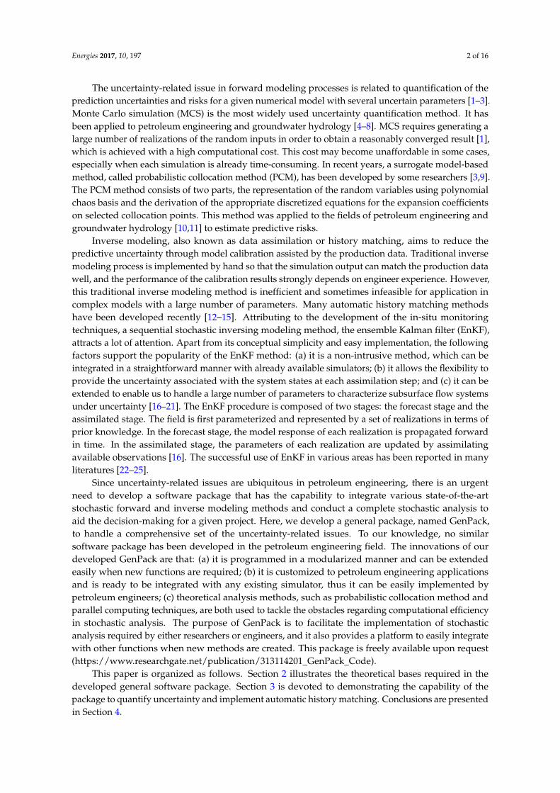
GenPack allows the user to apply the EnKF method to implement the inverse modeling process.We will validate inverse modeling module in GenPack based on the test case described in the previoussections. The model parameter values used in the synthetic reference case are listed in Table 2.The synthetic observation values, i.e., the producer BHP values and the injector BHP values rangedfrom 100 to 900 days, and are generated based on the reference model. The EnKF method is thencarried out to match the observations by optimally adjusting the model parameters. During the dataassimilation process, the ensemble size is set as 50, and the assimilation step is 50 day. Figure 9 depictsthe comparisons of the true values and initial realizations of model parameters before history matching.As shown in Figure 9, the 50 initial realizations of model parameters deviate from the true valuessignificantly. It indicates a relatively poor initial estimate of the model parameters. Figure 10 depictsthe mean predictions associated with their 95% confidence intervals (constructed using 50 predictionrealizations) on the basis of the initial realizations of model parameters. The mean predictionsdeviate from the reference or true values dramatically even though the true values are within theenvelope bounded by the upper and lower confidence intervals. Furthermore, the predictive variancerepresented by the width of the confidence intervals is relatively large, which indicates that there arerelatively large uncertainties associated with the predictions.

Table 2. The parameters used in the reference case.

Parameters Layer True Value

Porosity 1–3 0.3Permeability 1 500 mDPermeability 2 60 mDPermeability 3 200 mD

Energies 2017, 10, 197 12 of 16

validate inverse modeling module in GenPack based on the test case described in the previous sections. The model parameter values used in the synthetic reference case are listed in Table 2. The synthetic observation values, i.e., the producer BHP values and the injector BHP values ranged from 100 to 900 days, and are generated based on the reference model. The EnKF method is then carried out to match the observations by optimally adjusting the model parameters. During the data assimilation process, the ensemble size is set as 50, and the assimilation step is 50 day. Figure 9 depicts the comparisons of the true values and initial realizations of model parameters before history matching. As shown in Figure 9, the 50 initial realizations of model parameters deviate from the true values significantly. It indicates a relatively poor initial estimate of the model parameters. Figure 10 depicts the mean predictions associated with their 95% confidence intervals (constructed using 50 prediction realizations) on the basis of the initial realizations of model parameters. The mean predictions deviate from the reference or true values dramatically even though the true values are within the envelope bounded by the upper and lower confidence intervals. Furthermore, the predictive variance represented by the width of the confidence intervals is relatively large, which indicates that there are relatively large uncertainties associated with the predictions.

Table 2. The parameters used in the reference case.

Parameters Layer True ValuePorosity 1–3 0.3

Permeability 1 500 mD Permeability 2 60 mD Permeability 3 200 mD

(a) (b)

(c) (d)

Figure 9. The parameter values before history matching: (a) Porosity; (b) Permeability in layer 1; (c) Permeability in layer 2; and (d) Permeability in layer 3. Figure 9. The parameter values before history matching: (a) Porosity; (b) Permeability in layer 1;

(c) Permeability in layer 2; and (d) Permeability in layer 3.

Energies 2017, 10, 197 13 of 16

Energies 2017, 10, 197 13 of 16

(a) (b)

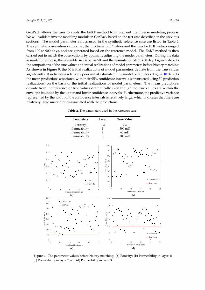
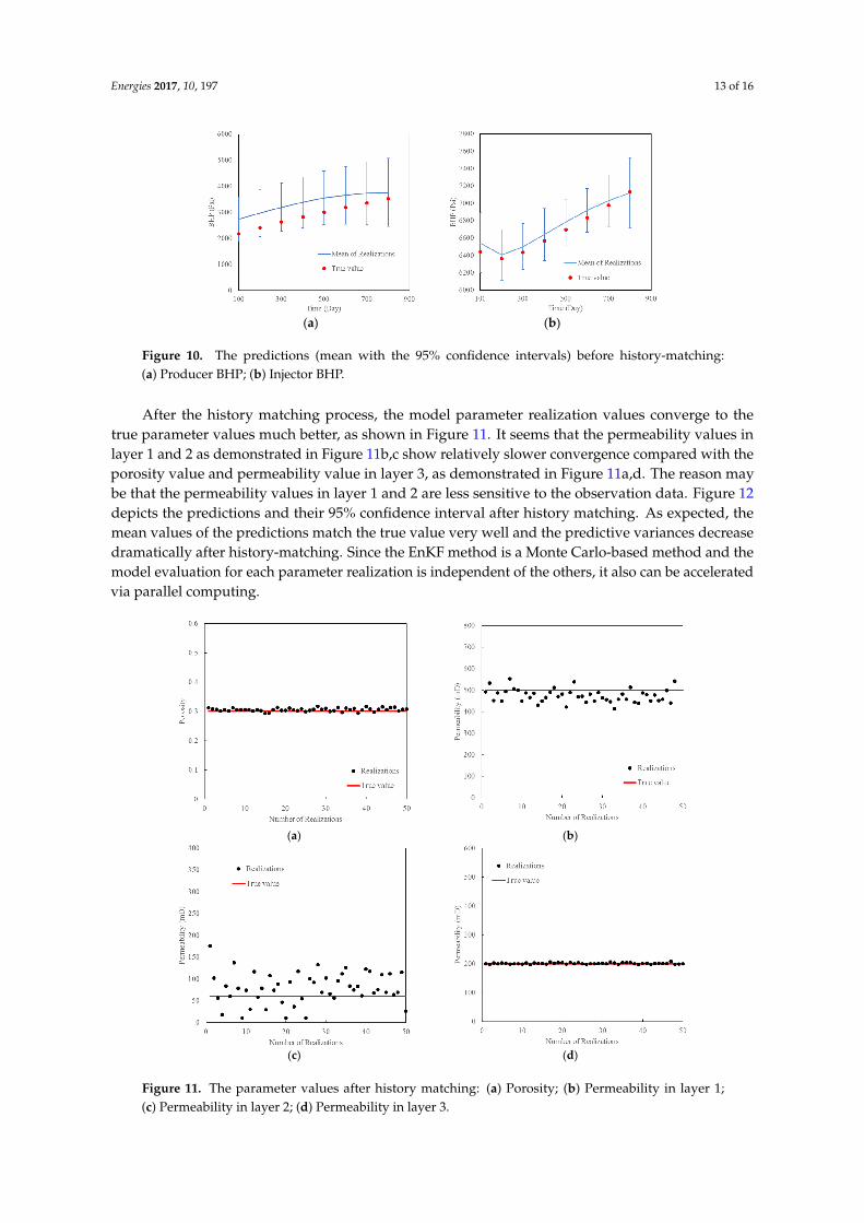
Figure 10. The predictions (mean with the 95% confidence intervals) before history-matching: (a) Producer BHP; (b) Injector BHP.

After the history matching process, the model parameter realization values converge to the true parameter values much better, as shown in Figure 11. It seems that the permeability values in layer 1 and 2 as demonstrated in Figure 11b,c show relatively slower convergence compared with the porosity value and permeability value in layer 3, as demonstrated in Figure 11a,d. The reason may be that the permeability values in layer 1 and 2 are less sensitive to the observation data. Figure 12 depicts the predictions and their 95% confidence interval after history matching. As expected, the mean values of the predictions match the true value very well and the predictive variances decrease dramatically after history-matching. Since the EnKF method is a Monte Carlo-based method and the model evaluation for each parameter realization is independent of the others, it also can be accelerated via parallel computing.

(a) (b)

(c) (d)

Figure 11. The parameter values after history matching: (a) Porosity; (b) Permeability in layer 1; (c) Permeability in layer 2; (d) Permeability in layer 3.

Figure 10. The predictions (mean with the 95% confidence intervals) before history-matching:(a) Producer BHP; (b) Injector BHP.

After the history matching process, the model parameter realization values converge to thetrue parameter values much better, as shown in Figure 11. It seems that the permeability values inlayer 1 and 2 as demonstrated in Figure 11b,c show relatively slower convergence compared with theporosity value and permeability value in layer 3, as demonstrated in Figure 11a,d. The reason maybe that the permeability values in layer 1 and 2 are less sensitive to the observation data. Figure 12depicts the predictions and their 95% confidence interval after history matching. As expected, themean values of the predictions match the true value very well and the predictive variances decreasedramatically after history-matching. Since the EnKF method is a Monte Carlo-based method and themodel evaluation for each parameter realization is independent of the others, it also can be acceleratedvia parallel computing.

Energies 2017, 10, 197 13 of 16

(a) (b)

Figure 10. The predictions (mean with the 95% confidence intervals) before history-matching: (a) Producer BHP; (b) Injector BHP.

After the history matching process, the model parameter realization values converge to the true parameter values much better, as shown in Figure 11. It seems that the permeability values in layer 1 and 2 as demonstrated in Figure 11b,c show relatively slower convergence compared with the porosity value and permeability value in layer 3, as demonstrated in Figure 11a,d. The reason may be that the permeability values in layer 1 and 2 are less sensitive to the observation data. Figure 12 depicts the predictions and their 95% confidence interval after history matching. As expected, the mean values of the predictions match the true value very well and the predictive variances decrease dramatically after history-matching. Since the EnKF method is a Monte Carlo-based method and the model evaluation for each parameter realization is independent of the others, it also can be accelerated via parallel computing.

(a) (b)

(c) (d)

Figure 11. The parameter values after history matching: (a) Porosity; (b) Permeability in layer 1; (c) Permeability in layer 2; (d) Permeability in layer 3.

Figure 11. The parameter values after history matching: (a) Porosity; (b) Permeability in layer 1;(c) Permeability in layer 2; (d) Permeability in layer 3.

Energies 2017, 10, 197 14 of 16Energies 2017, 10, 197 14 of 16

(a) (b)

Figure 12. The predictions (mean with the 95% confidence intervals) after history-matching: (a) Producer BHP; (b) Injector BHP.

4. Conclusions

This work can lead to the following major conclusions:

(1) Uncertainty-related issues are extremely important to aid the decision-making process in petroleum engineering. It is imperative to develop an efficient tool to quantify the risks and calibrate the simulation models. In this study, we designed a comprehensive general package, named GenPack to integrate together uncertainty quantification in forward modeling and uncertainty reduction in inverse modeling. GenPack is a helpful tool for petroleum engineers and researchers to effectively investigate the uncertainty-related issues in practice. In the current version of GenPack, the selected methods are either widely accepted or performed well in the existing literature. Other methods can be incorporated when they become available due to the modularized design of this package.

(2) GenPack allow user to generate Gaussian random fields via either KL expansion or sequential Gaussian simulation method. In order to improve the computational efficiency, one should decide how many leading terms can be retained in KL expansion. Sequential Gaussian simulation method is found to be suitable for parameter field generation in a large model with complex geometric boundaries.

(3) MCS and PCM are the options in GenPack to quantify uncertainty. MCS is a robust method for uncertainty quantification even though it requires large number of samples to guarantee the convergence. PCM is an efficient method to quantify uncertainty. The appropriate order of PCM can be investigated to achieve the balance between efficiency and accuracy during the analysis process.

(4) History matching is an important function in GenPack to assist us to take advantage of the observation data. GenPack applies the EnKF method in history matching. The method is validated with a synthetic case. The results show that the prediction accuracy can be greatly improved and the predictive uncertainty can be dramatically reduced after the implementation of history matching.

(5) GenPack is a Monte Carlo-based non-intrusive software package ready to be incorporated with any existing simulator in the petroleum engineering field. Due to the independence characteristics when evaluating each realization in the MC process, the efficiency of the stochastic analysis can be further improved with parallel computing when the required computing source is available.

Figure 12. The predictions (mean with the 95% confidence intervals) after history-matching:(a) Producer BHP; (b) Injector BHP.

4. Conclusions

This work can lead to the following major conclusions:

(1) Uncertainty-related issues are extremely important to aid the decision-making process inpetroleum engineering. It is imperative to develop an efficient tool to quantify the risks andcalibrate the simulation models. In this study, we designed a comprehensive general package,named GenPack to integrate together uncertainty quantification in forward modeling anduncertainty reduction in inverse modeling. GenPack is a helpful tool for petroleum engineersand researchers to effectively investigate the uncertainty-related issues in practice. In the currentversion of GenPack, the selected methods are either widely accepted or performed well in theexisting literature. Other methods can be incorporated when they become available due to themodularized design of this package.

(2) GenPack allow user to generate Gaussian random fields via either KL expansion or sequentialGaussian simulation method. In order to improve the computational efficiency, one shoulddecide how many leading terms can be retained in KL expansion. Sequential Gaussian simulationmethod is found to be suitable for parameter field generation in a large model with complexgeometric boundaries.

(3) MCS and PCM are the options in GenPack to quantify uncertainty. MCS is a robust methodfor uncertainty quantification even though it requires large number of samples to guaranteethe convergence. PCM is an efficient method to quantify uncertainty. The appropriate orderof PCM can be investigated to achieve the balance between efficiency and accuracy during theanalysis process.

(4) History matching is an important function in GenPack to assist us to take advantage of theobservation data. GenPack applies the EnKF method in history matching. The method isvalidated with a synthetic case. The results show that the prediction accuracy can be greatlyimproved and the predictive uncertainty can be dramatically reduced after the implementationof history matching.

(5) GenPack is a Monte Carlo-based non-intrusive software package ready to be incorporated withany existing simulator in the petroleum engineering field. Due to the independence characteristicswhen evaluating each realization in the MC process, the efficiency of the stochastic analysis canbe further improved with parallel computing when the required computing source is available.

Energies 2017, 10, 197 15 of 16

Acknowledgments: This work is funded by the National Natural Science Foundation of China (Grant No.41402199), National Science and Technology Major Project (Grant No. 2016ZX05037003, 2016ZX05060002),the Science Foundation of China University of Petroleum—Beijing (Grant No. 2462014YJRC038), the independentresearch funding of State Key Laboratory of Petroleum Resources and Prospecting (Grant No. PRP/indep-4-1409),China Postdoctoral Science Foundation (Grant No. 2016M591353), and the Science Foundation of Sinopec Group(Grant No. P16063).

Author Contributions: Cheng Dai developed the GenPack software package; Liang Xue performed the synthetictests and wrote the paper; Lei Wang designed the parallel computing.

Conflicts of Interest: The authors declare no conflict of interest

References

1. Zhang, D. Stochastic Methods for Flow in Porous Media: Coping with Uncertainties; Academic Press: New York,NY, USA, 2001.

2. Xiu, D. Numerical Methods for Stochastic Computations: A Spectral Method Approach; Princeton University Press:Princeton, NJ, USA, 2010.

3. Xiu, D.; Karniadakis, G.E. The Wiener–Askey polynomial chaos for stochastic differential equations. SIAM J.Sci. Comput. 2002, 24, 619–644. [CrossRef]

4. Bakr, A.A.; Gelhar, L.W.; Gutjahr, A.L.; Macmillan, J.R. Stochastic analysis of spatial variability in subsurfaceflows: 1. Comparison of one- and three-dimensional flows. Water Resour. Res. 1978, 14, 263–271. [CrossRef]

5. Gelhar, L.W. Stochastic subsurface hydrology from theory to applications. Water Resour. Res. 1986, 22.[CrossRef]

6. James, A.L.; Oldenburg, C.M. Linear and Monte Carlo uncertainty analysis for subsurface contaminanttransport simulation. Water Resour. Res. 1997, 33, 2495–2508. [CrossRef]

7. Kuczera, G.; Parent, E. Monte Carlo assessment of parameter uncertainty in conceptual catchment models:The Metropolis algorithm. J. Hydrol. 1998, 211, 69–85. [CrossRef]

8. Liu, N.; Oliver, D.S. Evaluation of Monte Carlo methods for assessing uncertainty. SPE J. 2003, 8, 188–195.[CrossRef]

9. Xiu, D.; Karniadakis, G.E. Modeling uncertainty in flow simulations via generalized polynomial chaos.J. Comput. Phys. 2003, 187, 137–167. [CrossRef]

10. Li, H.; Zhang, D. Probabilistic collocation method for flow in porous media: Comparisons with otherstochastic methods. Water Resour. Res. 2007, 43. [CrossRef]

11. Li, H.; Zhang, D. Efficient and accurate quantification of uncertainty for multiphase flow with theprobabilistic collocation method. SPE J. 2009, 14, 665–679. [CrossRef]

12. Romero, C.E.; Carter, J.N. Using genetic algorithms for reservoir characterisation. J. Pet. Sci. Eng. 2001, 31,113–123. [CrossRef]

13. Dong, Y.; Oliver, D.S. Quantitative use of 4D seismic data for reservoir description. In Proceedings of theSPE Annual Technical Conference and Exhibition, Denver, CO, USA, 5–8 October 2003.

14. Gao, G.; Reynolds, A.C. An improved implementation of the LBFGS algorithm for automatic historymatching. In Proceedings of the SPE Annual Technical Conference and Exhibition, Houston, TX, USA,26–29 September 2004.

15. Ballester, P.J.; Carter, J.N. A parallel real-coded genetic algorithm for history matching and its application toa real petroleum reservoir. J. Pet. Sci. Eng. 2007, 59, 157–168. [CrossRef]

16. Chen, Y.; Zhang, D. Data assimilation for transient flow in geologic formations via ensemble Kalman filter.Adv. Water Resour. 2006, 29, 1107–1122. [CrossRef]

17. Oliver, D.S.; Reynolds, A.C.; Liu, N. Inverse Theory for Petroleum Reservoir Characterization and History Matching;University Press: Cambridge, UK, 2008.

18. Liu, G.; Chen, Y.; Zhang, D. Investigation of flow and transport processes at the MADE site using ensembleKalman filter. Adv. Water Resour. 2008, 31, 975–986. [CrossRef]

19. Aanonsen, S.; Nævdal, G.; Oliver, D.; Reynolds, A.; Vallès, B. The Ensemble Kalman Filter in ReservoirEngineering—A review. SPE J. 2009, 14, 393–412. [CrossRef]

20. Xie, X.; Zhang, D. Data assimilation for distributed hydrological catchment modeling via ensemble Kalmanfilter. Adv. Water Resour. 2010, 33, 678–690. [CrossRef]

Energies 2017, 10, 197 16 of 16

21. Dai, C.; Xue, L.; Zhang, D.; Guadagnini, A. Data-worth analysis through probabilistic collocation-basedEnsemble Kalman Filter. J. Hydrol. 2016, 540, 488–503. [CrossRef]

22. Lorentzen, R.J.; Naevdal, G.; Valles, B.; Berg, A.; Grimstad, A.-A. Analysis of the ensemble Kalman filter forestimation of permeability and porosity in reservoir models. In Proceedings of the SPE Annual TechnicalConference and Exhibition, San Antonio, TX, USA, 24–27 September 2006.

23. Gao, G.; Reynolds, A.C. An improved implementation of the LBFGS algorithm for automatic historymatching. SPE J. 2006, 11, 5–17. [CrossRef]

24. Gu, Y.; Oliver, D.S. History Matching of the PUNQ-S3 Reservoir Model Using the Ensemble Kalman Filter.SPE J. 2005, 10, 217–224. [CrossRef]

25. Liao, Q.; Zhang, D. Probabilistic collocation method for strongly nonlinear problems: 1. Transform bylocation. Water Resour. Res. 2013, 49, 7911–7928. [CrossRef]

26. Wiener, N. The Homogeneous Chaos. Am. J. Math. 1938, 60, 897–936. [CrossRef]27. Ghanem, R.G.; Spanos, P.D. Stochastic Finite Elements: A Spectral Approach; Courier Corporation: Chelmsford,

MA, USA, 2003.28. Li, H.; Sarma, P.; Zhang, D. A Comparative Study of the Probabilistic-Collocation and Experimental-Design

Methods for Petroleum-Reservoir Uncertainty Quantification. SPE J. 2011, 16, 429–439. [CrossRef]29. Ghanem, R. Scales of fluctuation and the propagation of uncertainty in random porous media.

Water Resour. Res. 1998, 34, 2123–2136. [CrossRef]30. Mathelin, L.; Hussaini, M.Y.; Zang, T.A. Stochastic approaches to uncertainty quantification in CFD

simulations. Numer. Algorithms 2005, 38, 209–236. [CrossRef]31. Tatang, M.A.; Pan, W.; Prinn, R.G.; McRae, G.J. An efficient method for parametric uncertainty analysis of

numerical geophysical models. J. Geophys. Res. Atmos. 1997, 102, 21925–21932. [CrossRef]32. Deutsch, C.V.; Journel, A.G. GSLIB: Geostatistical Software Library and User’s Guide, 2nd ed.;

Applied Geostatistics Series; Oxford University Press: New York, NY, USA, 1998.

© 2017 by the authors; licensee MDPI, Basel, Switzerland. This article is an open accessarticle distributed under the terms and conditions of the Creative Commons Attribution(CC BY) license (http://creativecommons.org/licenses/by/4.0/).