JOURNAL OF GEOPHYSICAL RESEARCH, VOL. 104, NO. C5, PAGES 11,273-11,289, MAY 15, 1999

Uncertainty of South China Sea prediction using NSCAT and National Centers for Environmental

Prediction winds during tropical storm Ernie 1996

Peter C. Chu

Department of Oceanography, Naval Postgraduate School, Monterey, California

Shihua Lu

Institute of Plateau Atmospheric Physics, Academia Sinica, Lanzhou, China

W. Timothy Liu Jet Propulsion Laboratory, Pasadena, California

Abstract. Error propagation from winds to ocean models was numerically investigated using the Princeton Ocean Model (POM) for the South China Sea with 20-km horizontal resolution and 23 • levels conforming to a realistic bottom topography during the lifetime of tropical cyclone Ernie (November 4-18, 1996). Numerical integration was divided into preexperimental and experimental stages. The preexperiment phase generates the initial conditions on November i for the sensitivity experiment. During the experimental stage the POM was integrated from November 1 to 30, 1996 under National Centers for Environmental Prediction (NCEP) reanalyzed surface fluxes along with two surface wind data sets, namely, the daily averaged interpolated NASA scatterometer winds and the NCEP winds. The relative root-mean-square differences fluctuate from 0.5 to 1.0 for winds, 0.25 to 0.7 for surface elevations, 0.47 to 1.02 for surface currents, and 0 to 0.23 for aurface temperatures. This indicates that the model has less uncertainty overall than the wind fields used to drive it, which in turn suggests that the ocean modeling community may progress without waiting for the atmospheric modelers to build the perfect forecast model.

1. Introduction

Several important questions in ocean modeling need to be answered: How does error propagate from winds to ocean? Will the wind error be amplified or damped after it enters the ocean models? A possible way to deal with these problems is to run an ocean model with two different wind data sets, then to analyze the variability of the two ocean model fields versus the variability of the two wind fields. Here we chose the Princeton Ocean

Model (POM)for the South China Sea (SCS)for such a study.

The SCS is a semienclosed, tropical sea located be- tween the Asian land mass to the north and west, the Philippine Islands to the east, Borneo to the southeast, and Indonesia to the south (Figure 1), a total area of 3.5 x 10 c km e. It includes the shallow Gulf of Thai-

land and connections to the East China Sea (through the Taiwan Strait), to the Pacific Ocean (through the

Copyright 1999 by the American Geophysical Union.

Paper number 1998JC900046. 0148-0227/99/1998JC900046509.00

Luzon Strait), to the Sulu Sea (through the Mindoro Strait), to the Java Sea (through the Gasper and Kari- mata Straits), and to the Indian Ocean (through the Strait of Malacca). All of these straits are shallow, ex- cept the Luzon Strait, whose maximum depth is 1800 m. The complex topography includes the broad shallows of the Sunda Shelf in the south/southwest; the continen- tal shelf of the Asian landmass in the north, extending from the Gulf of Tonkin to the Taiwan Strait; a deep, elliptical shaped basin in the center, and numerous reef islands and underwater plateaus scattered throughout. The shelf that extends from the Gulf of Tonkin to the Taiwan Strait is consistently near 70 m deep and av- erages 150 km in width; the central deep basin is 1900 km along its major axis (northeast-southwest) and ap- proximately 1100 km along its minor axis and extends to over 4000 m deep. The Sunda Shelf is the submerged connection between southeast Asia, Malaysia, Sumatra, Java, and Borneo and is 100 m deep in the middle; the center of the Gulf of Thailand is about 70 m deep.

The SCS is subjected to a seasonal monsoon sys- tem [Wyrtki, 1961; Chu et al., 1997a, 1998a; Metzget

11,273

11,274 CHU ET AL.- UNCERTAINTY OF SOUTH CHINA SEA PREDICTION

25

2O

15

100 105 • 0 115 120 125 130 135

Longitude (E) Figure 1. Bathymetry (meter) and coastline of the South China Sea (SCS).

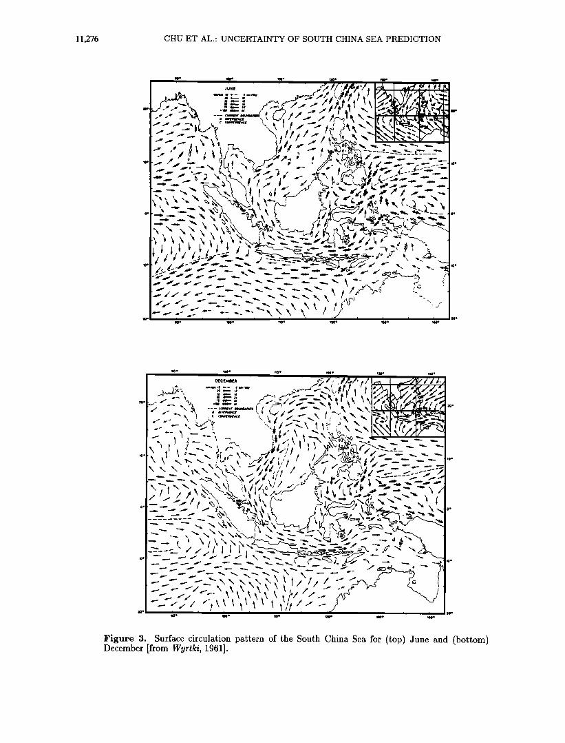
and Hurlburr, 1996]. From April to August the weaker southwesterly summer monsoon winds result in a wind stress of more than 0.1 N m -2 (Figure 2a), which drives a northward coastal jet off Vietnam and anticyclonic circulation in the SCS (Figure 3, top). From November to March the stronger northeasterly winter monsoon winds correspond to a maximum wind stress of nearly 0.28 N m -2 (Figure 2b), causing a southward coastal jet and cyclonic circulation in the SCS (Figure 3, bottom). The transitional periods are marked by highly variable winds and surface currents.

More tropical cyclones form over the western North Pacific and SCS regions than in any other ocean basin, with an average of about 26 per year [McBride, 1995]. Although highly seasonal, this is the only region in which tropical cyclones have been observed in all months of the year. The primary reason for this high incidence of occurrence is the persistently warm sea surface tem- peratures (SST) and the location of the intertropical convergence zone (ITCZ). The ITCZ occurs as a conver- gence zone in the westerly monsoon flow, known as the monsoon trough [Gray, 1968]. The trough is the shear line separating the monsoonal westerlies from the trade easterlies and is a preferred region for tropical cyclone development. The tropical cyclone Ernie in 1996 was selected since it traveled through the whole SCS dur- ing November 1996. More importantly, we have both satellite and reanalyzed wind data for the duration of tropical cyclone Ernie.

The National Aeronautics and Space Administra- tion (NASA)scatterometer (NSCAT) was successfully launched into a near-polar and Sun-synchronous or- bit on the Japanese Advanced Earth Observing Satel- lite (ADEOS 1) in August 1996. About 9 months of data were collected before the failure of ADEOS. From

NSCAT observations, surface wind vectors (speed and direction) at 10-m height were derived at 25-km spatial resolution, covering approximately 77% of the Earth's oceans in i day and 87% in 2 days, under both clear and cloudy conditions. The NSCAT observations were in- terpolated objectively by the method of successive cor- rections to form a uniformly gridded wind field, with 0.50 latitude by 0.5 o longitude and 12-hour resolution [Tang and Liu, 1996; Liu et al., 1998].

Two surface wind data sets were chosen for the study, namely, the NSCAT winds and the National Centers for Environmental Prediction (NCEP) T63 (equivalent to 1.875 ø x 1.875 ø resolution) reanalyzed winds. The daily mean data were used for simplicity since we are only interested in the error propagation.

The outline of this paper is as follows. A description of tropical cyclone Ernie 1996 is given in section 2. A depiction of numerical experiments is given in section 3. Statistical analyses are presented in section 4. Dis- crepancy between NSCAT and NCEP surface winds is described in section 5. SCS model response is given in section 6. In section 7 we present our conclusions.

CHU ET AL.' UNCERTAINTY OF SOUTH CHINA SEA PREDICTION 11,275

(a) June

i1•-'.-•....:•:• .ii?ii•i•i•---:•:• --t••i•'....•,,, ,. ..... ß ..... .,, .• .... .•,•,y....••-,: ..... ß .... ,., .... ß ..... .,,

-- ••, ,•,,: ..... :. ,,,: ..... : ..... :,, • ••_,, ,.,, ,,,.,, .... •;, ................

I.•: - --'-••- ,,,, ,.,,, ,•, .•,• ............. •0oU• .. • •-.• •.,.• , •.,.,. ,., .,.,/;:....-•,•:•..: ..-....: • ......::

I• .............. "' '• ...... '• ............

;:;; ;,; ;:;; • ' . :::::::::::::::::::::

-••: ..... : ........ : ..... :,,,• ,:... ' 100øE 105øE 110øE 115øE 120øE 125øE 130øE 135øE

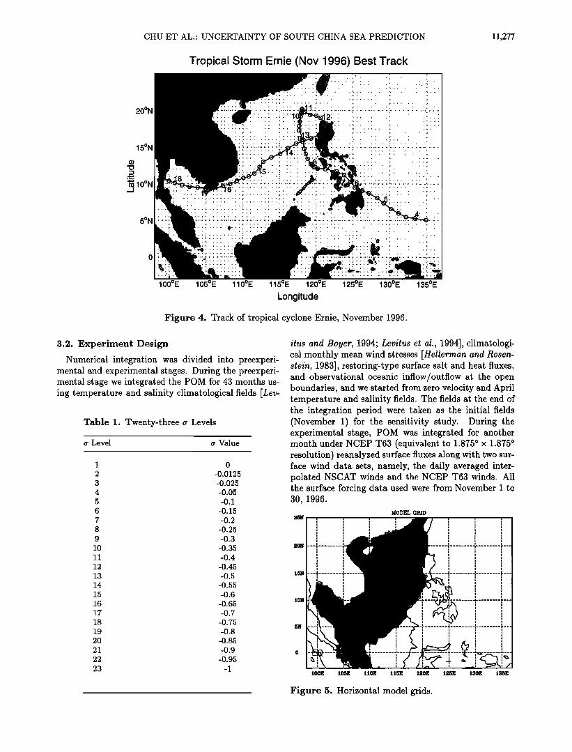
ous day, began interacting with Ernie at this tinge, a•nd late on November 8, Ernie began moving northerly to- ward this circulation. Ernie merged with TD 39W and continued moving northerly, slowly intensifying from its low wind speed of 15 m s-1 after merger to 23 m s -1. On November 11, midlevel steering flow again dimin- ished and Ernie commenced slowly drifting southerly toward Luzon, approximately 270 km to the southeast. On November 12, Ernie was over Luzon and midlevel steering flow reintensified, causing the system to begin moving to the west-southwest, back into the SCS. Ernie continued moving to the west-southwest over the next 4 days, passing over the southern tip of Vietnam and slowly weakening to 15 m s -1. Ernie tracked into the Gulf of Thailand and then finally into the eastern Bay of Bengal, where it dissipated over water on November 18.

(b) December ............ /'-•• ß r/,/, •. z./; ,' z • • ,' ,'-,' ,' '-:• • ; Z//'';"''';" , ß ;K/Z/t/Y/Y/,'/

//' '• ' •'•,',,- .•',,' 15ON • •.7.7'/'Y.7•'Y't ! ,•..""•

• .•' v'/'/•Y.2;':. z.- .z.•.: •: ,•///,',','.'.'.'-'-'

I:. • ,,z... ,(. v../'.'./':z. v. z. ,, z, :.•i'.". .... ,•. ", ' ........... $øNr.'.•.'.?,'.,'.•,'•.•.'••.., •. • • •.,,,,,, ;.'•,,.![ ':':' • ".i'.':"; '.':!:' • :.':':'i • ",

!•••', :',',•', ',_:', ',•••I•: :" .... ' ..... ' ........

I '"'•I•"-, ','" ', ' -' .•• - -..••••'-' _•,•-. '.•_5.: '. :.': •','-'-:•"•• :: k'-

100øE 105øE 110øE 115øE 120øE 125øE 130øE 135øE

Figure 2. Climatological wind stress (N m -2) for (a) June and (b) December.

2. Tropical Cyclone Ernie, 1996 Tropical cyclone Ernie formed initially about 1300

km to the east of the Philippine island of Mindanao on November 4, 1996. After formation, Ernie slowly intensified as it tracked westward through the Philip- pine Sea toward the central Philippine islands. Figure 4 shows the track of Ernie, which was obtained from the Joint Typhoon Warning Center (JTWC) on Guam. On November 6, Ernie made landfall over Mindanao and intensified to 18 m s-1, tropical storm strength. Ernie continued moving westerly through the Philippine Is- lands, intensifying at a slow rate owing to interaction with the land. The storm entered the SCS on November

7 and reached an intensity of 25 m s-•. On November 8, Ernie became quasi-stationary over the eastern SCS and began losing intensity when midlevel steering flow di- minished and a strong, low-level monsoonal flow devel- oped. Tropical depression (TD) 39W, which had formed over Luzon to the northeast of Ernie during the previ-

3. Numerical Experiments

3.1. Model Description

POM is the three-dimensional primitive equation model developed by Blumberg and Mellor [1987] with hydro- static and Boussinesq approximations and has the fol- lowing features: (1) a staggered C grid, (2) er coordi- nates in the vertical, (3) a free surface, (4) a second- order turbulence closure model for vertical viscosity [Mellor and Yamada, 1982], (5)horizontal diffusivity coefficients calculated by the $magorin•ky [1963] pa- rameterization, and (6) split time steps for barotropic (25 s) and baroclinic modes (900 s).

The model was specifically designed to accommodate mesoscale phenomena commonly found in estuarine and coastal oceanography. Tidal forcing and river outflow were not included in this application of the model. How- ever, the seasonal variation in sea surface height, tem- perature, salinity, circulation, and transport are well represented by the model data. From a series of nu- merical experiments [Chu et al., 1998b], the effects of wind forcing and lateral boundary transport on the SCS warm-core and cool-core eddies are analyzed, yielding considerable insight into the external factors affecting the region oceanography.

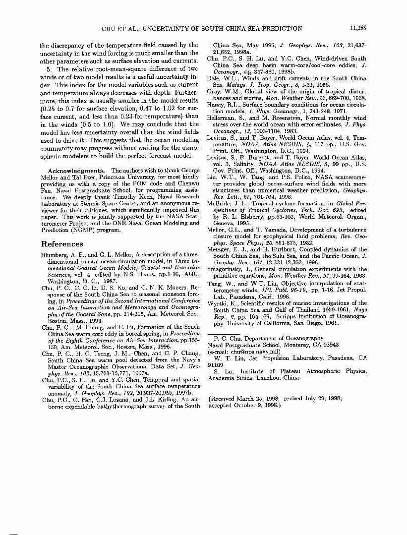
In this study we use a rectilinear grid with hori- zontal spacing of 20 km by 20 km resolution and 23 nonuniform vertical a coordinate levels (Table 1). The model domain is from 3.06øS to 25.07øN and 98.84øE to

121.16øE, which encompasses the SCS and the Gulf of Thailand, and uses realistic bathymetry data from the Naval Oceanographic Office Digital Bathymetry Data Base with 5 min by 5 min resolution (DBDB5). Conse- quently, the model contains 125 x 162 x 23 horizontally fixed grid points (Figure 5). The horizontal diffusivities are modeled using the •'magorinsky [1963] form, with the coefficient chosen to be 0.2 for this application. The bottom stress is assumed to follow a quadratic law, and the drag coefficient is specified as 0.0025 [Blumberg and Mellor, 1987].

11,276 CHU ET AL.' UNCERTAINTY OF SOUTH CHINA SEA PREDICTION

.... --,,. -- '--,,,,,, ,,,_,,, ',,5 •t.,, I- / -" ':'._•-x ? Y• • ..--.' =... '"--- \ •, -- / ...,. ..,. •

i i I i i i i i i i i i tO ß I00 ß I•0 ß •0 ß GO e •0 ß

Figure 3. Surface circulation pattern of the South China Sea for (top) June and (bottom) December [from 14/yrtki, lgOl].

CHU ET AL.' UNCERTAINTY OF SOUTH CHINA SEA PREDICTION 11,277

20ON --

15øN

'• 10øN

5øN

Tropical Storm Ernie (Nov 1996) Best Track .... ..:.. ........ : ......... : ß . .

...............................

....... ß ......... • ......... : ...

100øE 105øE 110øE 115øE 120øE 125øE 130øE 135øE

Longitude

Figure 4. Track of tropical cyclone Ernie, November 1996.

3.2. Experiment Design

Numerical integration was divided into preexperi- mental and experimental stages. During the preexperi- mental stage we integrated the POM for 43 months us- ing temperature and salinity climatological fields [Lev-

Table 1. Twenty-three •r Levels

Level er Value

1 0

2 -0.0125

3 -0.025

4 -0.05

5 -0.1

6 -0.15

7 -0.2

8 -0.25

9 -0.3

10 -0.35

11 -0.4

12 -0.45

13 -0.5

14 -0.55

15 -0.6

16 -0.65

17 -0.7

18 -0.75

19 -0.8

20 -0.85

21 -0.9

22 -0.95

23 -1

itus and Boyer, 1994; Levitus et al., 1994], climatologi- cal monthly mean wind stresses [Hell.errnan and Rosen- stein, 1983], restoring-type surface salt and heat fluxes, and observational oceanic inflow/outflow at the open boundaries, and we started from zero velocity and April temperature and salinity fields. The fields at the end of the integration period were taken as the initial fields (November 1) for the sensitivity study. During the experimental stage, POM was integrated for another month under NCEP T63 (equivalent to 1.875 o x 1.875 o resolution) reanalyzed surface fluxes along with two sur- face wind data sets, namely, the daily averaged inter- polated NSCAT winds and the NCEP T63 winds. All the surface forcing data used were from November i to 30, 1996.

MODEL GRID 25N , ,

I0N

5N

'" I

130E 135E

Figure 5. Horizontal model grids.

11,278 CHU ET AL.' UNCERTAINTY OF SOUTH CHINA SEA PREDICTION

Table 2. Bimonthly Variation of Volume Transport at Lateral Open Boundaries

Feb. April June Aug. Oct. Dec.

Gaspar- Karimata Straits 4.4 0.0 -4.0 -3.0 1.0 4.3 Luzon Strait -3.5 0.0 3.0 2.5 -0.6 -3.4

Taiwan Strait -0.9 0.0 1.0 0.5 -0.4 -0.9

aValues are in Sverdrups. Positive/negative values mean outflow/inflow and were taken from Wyrtki [1961].

3.3. Atmospheric Forcing

3.3.1. Wind forcing. The atmospheric forcing for the SCS application of the POM includes mechan- ical and thermodynamic forcing. The wind forcing is depicted by

poKM(OU/OZ, OvlOz)z=o -- (v0x;v0y) (1)

where (u, v)and (v0•, v0y)are the two components of the water velocity and wind stress vectors, respectively; p0 is the reference density; and KM is the vertical mix- ing coefficient for momentum.

From a climatological point of view the SCS ex- periences two monsoons, winter and summer, every year. During the winter monsoon season a cold north- east wind blows over the SCS (Figure 2a) as a result of the Siberian high-pressure system located over the east Asian continent. Radiative cooling and persistent cold air advection maintain cold air over the SCS. The

northeast-southwest oriented jet stream is positioned at the central SCS. Such a typical winter monsoon pattern lasts nearly 6 months (November to April). During the summer monsoon season a warm and weaker southwest

wind blows over SCS (Figure 2b). Such a typical sum-

mer monsoon pattern lasts nearly 4 months (mid-May to mid-September).

During the preexperiment stage the wind stress at each time step is interpolated from monthly mean cli- mate wind stress [Hellerman and Rosenstein, 1983], which was taken as the value at the middle of the month.

During the experiment stage we used the two daily sur- face wind data sets (NSCAT and NCEP) to force the SCS POM model.

3.3.2. Thermohaline forcing. Surface thermal forcing is depicted by

O0 Q---•--• ) + a.(0o•s - o) (2) K H •z Z -- (•1(

Ks•z z - alQs + o•2C(SoBs - S) (3) where KH and Ks are the vertical mixing coefficients for temperature and salinity, respectively; OOBS and SOBS are the observed potential temperature and salinity, re- spectively; cp is the specific heat; and QH and Qs are surface net heat and salinity fluxes, respectively. The relaxation coefficient C is the reciprocal of the restoring time period for a unit volume of water. The parame-

1 1.5

1.2

5 n' 0.7

2- 0.5

2 -

1 (B) C .... , .... , .... . .... , .... , .............. , , i .... i ........ 5 10 15 20 25 30 '5 1'0 15 20 2'5 30

November 1996 November 1996

Figure 6. Temporally varying (a) root-mean-square difference (rmsd) and (b) relative root- mean-square difference (rrmsd) between daily mean NASA scatterometer (NSCAT) and National Centers fot Envirohmental Prediction (NCEP) winds over SCS.

CHU ET AL.: UNCERTAINTY OF SOUTH CHINA SEA PREDICTION 11,279

ters (c•, c•2) are (0,1)-type switches: c• - 1, c•2 - 0, would specify only if flux forcing is applied; c• - 0, c•2 - 1, would specify that only restoring-type forcing is applied. The relaxation coefficient C is taken to be 0.7 m day -•, which is equivalent to a relaxation time of 43 days for an upper layer 30 m thick [Chu at al., 1996]. Here we used restoring-type forcing for the pre- experiment (c• = 0, c•2 = 1) and flux forcing for the experiment (a• = 1, a• = 0.)

3.4. Lateral Boundary Conditions

Solid lateral boundaries, i.e., the modeled ocean bor- dered by land, were defined using a free slip condition for velocity and a zero gradient condition for tempera- ture and salinity. No advective or diffusive heat, salt, or velocity fluxes occur through these boundaries.

Open boundaries, where the numerical grid ends but the fluid motion is unrestricted, were treated as radia- tive boundaries. Volume transport through the Luzon Strait, Taiwan Strait, and Gasper/Karimata Strait was defined according to observations (Table 2). However, the Balabac Channel, Mindoro Strait, and Strait of Malacca are assumed to have zero transport. When the water flows into the model domain, temperature and salinity at the open boundary are likewise prescribed from the climatological data [Lavitus and Boyar, 1994]. When water flows out of the domain, the radiation con- dition was applied,

0(0 $)+v 0 0-7 ' s) - 0 (4)

where U• is the normal velocity at the boundary; and the subscript n is the direction normal to the boundary.

4. Statistical Analyses

The uncertainty of SCS in the two wind data sets was analyzed using correlation analysis and root-mean- square difference (rmsd). Let (xi, yj) and rr be the horizontal and vertical coordinates, respectively, of a model grid. For a given time t, let •P•scA? (xi, yj, rr, t) and ;b•½•.p(xi, yj, rr, t) represent two sets of wind and model output. For surface wind data and two-diemnsional output such as surface elevation, we set rr = O. Three parameters used to identify difference are root-mean- square (rms) difference, relative rms difference, and cor-

relation coefficient (CC). The rms difference represents the overall difference, the relative rms difference denotes the overall difference relative to the internal variability, and CC indicates the correlation between the two model

data sets. Discrepancy between the two data sets is characterized by large values of rms difference and low values of CC.

4.1. The rms Difference

The rms difference between •P•s½AT(xi, yj,er, t) and •NCgp(gri, yj, er, t) is defined by

rmsd,p ((r, t) -- • E IA•b(xi' YJ' (r, t)l 2 (5) ß .

$

where

t) = t) - t)

and M is the total number of horizontal grid points. The variable •p can be either scalar or vector (wind and current). If •p is a vector, I(X½)l in (5) means the mod- ulus of the vector A•p.

4.2. Relative rms Difference

The relative rms difference (rrmsd) is the ratio be- tween rmsd and standard deviation of the fields,

rrmsd ((r, t) -- rmsd ((r, t) (7) where the standard deviation $½(er, t) is computed by

S• (e r, t) - M - I E Y•- •P•c•.r ( x i , yj , er, t) - •P•c•.r (e r, t) ß ,

(s) Here the overbar () indicates the horizontal mean, and the variable •p can be either scalar or vector (wind and current).

4.3. Correlation Coefficient

The Pearson product-moment correlation coefficient between •P•s½aT(xi, yj, er, t) and •P•½•.r(xi, yj, er, t) is com- puted through all the SCS horizontal model grids,

Table 3. Maximum Root-Mean-Square Differences of Various Parameters and Dates of Occurrence

Maximum Value Date in November

Surface winds, m s- • 6.7 4 Surface elevation, cm 4.3 4, 30

Surface current, m s -• 0.18 30 T (a =-0.025), o C 0.52 30

11,280 CHU ET AL.' UNCERTAINTY OF SOUTH CHINA SEA PREDICTION

cc(, t) -

Since neither of the two model data sets is consid-

ered "true," the three parameters defined in this sec- tion, rmsd•(•, t), rrmsd• (tr, t), and CC(tr, t), cannot be considered as an error bias. They only show the differ- ence between the two model results.

5. Discrepancy Between NSCAT and NCEP Surface Winds in November 1996

Before analyzing the data, both daily averaged NCEP and NSCAT wind data were interpolated into the ocean model grids. Quite surprisingly, the difference between the two wind fields is not negligible. The rmsd (Figure 6a) increases from 3.6 m s -• on November i to a maxi- mum value of 6.7 m s -• on November 4, 1996 (Table 3), the day when the boundary current was strongest; and then fluctuates between 6.7 and 2.7 m s -•. The rrmsd

(Figure 6b) varies between 0.5 and 1, with a maximum value of 1.0 on November 12 (Table 4), indicating that the difference between the two wind data sets has the

same order of magnitude as the internal variability. The value of i for rrmsd means that the difference between

the two model results equals the model's internal vari- ability.

Figure 7 shows the comparison between NSCAT and NCEP winds on November 4, 12, and 15 when rmsd exceeds 5 m s -•. On November 4, both data sets show the establishment of the northeast monsoon in

the northern SCS (110ø-120øE, 16ø-25øN) and the re- treat of the southwest monsoon in the southern SCS.

However, the NSCAT winds show a stronger retreat of the southwest monsoon than the NCEP winds. In the

central SCS (5ø-18øN) the southwest monsoon disap- peared (appeared) in the NSCAT (NCEP) wind data. The difference between the two data sets has the same order of magnitude of the wind itself, i.e.• 10-20 m s -•. Moreover, the NCEP winds exhibit a strong conver- gence between the northeast and southwest monsoons near 14øN, but NSCAT winds do not. Such a large un- certainty on November 4 instead of when the cyclone was present may be associated with the monsoon re- versal. During November 9-13, Ernie was in the quasi-

stationary stage, looping around west of Luzon Island (Figure 4). On November 12, Ernie was located at the north tip of Luzon. Both winds show the existence of a cyclone centered at the north tip of Luzon. Ernie was much stronger in the NSCAT winds than in the NCEP winds. After November 12, Ernie moved toward Vietnam. On November 15, Ernie was located at 12øN, 112ø30'E (Figure 4). However, it was shifted toward south (8øN, 112øE) in both NSCAT and NCEP winds and was very weak in the NSCAT winds.

The correlation coefficient between daily NSCAT and NCEP wind components also fluctuates (Figure 8). Dur- ing the lifetime of Ernie (November 4-18, 1996), CC fluctuated between 0.6 and 0.9 for the u component and between 0.42 and 0.92 for the v component. The mini- mum CC was determined to be 0.42 for the latitudinal

component on November 4, 1996 (Table 5.)

6. SCS Model Response to the Uncertainty of Wind Forcing

Since the two surface wind data sets are quite differ- ent, we may ask how does the ocean respond to such a wind discrepancy? The emphasis here is to show the model uncertainty caused by the wind uncertainty. Thus we computed rmsd, rrmsd, and CC of model out- puts (surface elevation, currents, and temperature) us- ing NSCAT and NCEP winds to describe the uncer- tainty. We refer to the NSCAT run as the numerical simulation with the NSCAT winds and to the NCEP

run as the numerical simulation with the NCEP winds.

6.1. Surface Elevation

Figure 9 shows the comparison between two surface elevation fields under NSCAT and NCEP wind forcing on November 4, 12, and 15. As Ernie was generated east of the South China Sea on November 4, 1996 (Figure 9a), both runs simulated surface depression in the deep SCS basin with a maximum value of 6 cm and produced sea surface setups along the southeast Chinese coast. The difference between the two runs on November 4 is

Table 4. Maximum Relative Root-Mean-Square Differences of Various Parame- ters and Dates of Occurrence

Maximum Value Date in November

Surface winds 1.0 12

Surface elevation O. 7 12 Surface current 1.02 4

Sea surface temperature 0.23 18

CHU ET AL' UNCERTAINTY OF SOUTH CHINA SEA PREDICTION 11,281

20

10.

(a) NC7• •D (m/s) NOV 4

o.eoo•+o• ' ••2 2 • • t •

..... It IIl•'' ,,

X • • '.• / / •

20

10

0

(b)

20

lO

o

100E "•1'i0E 120E 100E 110E 120E 100E 110E 120--

NSCA•T WIND (m/s) NOV 4 . NSCAT WIND (m/-) NOV le ,/, NSOAT • (m/,) NOV •5 , //

0.2 0 •00•+02 I t t t I • • / n •nn.•n•/•/////•/' '• I

'" J• •!•E •': ": :---:x ...... :::::7.

. .

I•E 11 •E 1 2•E 1 •E 1 I•E 1 2•E I•E 1 I•E 1 2•E

20 20 20 • ••'; ....

I

I t •l/lt•(• ..... ,ll•

1 00E "i'1 OE 1 20E 1 00E 11 OE 1 20E 1 00E 110E 1 20E

Figure 7. Comparison between interpolated NSCAT and NCEP wind vectors on November (a) 4, (b) 12, and (c) 15.

11,282 CHU ET AL.' UNCERTAINTY OF SOUTH CHINA SEA PREDICTION

0.75

1,,,.i,,',1 .... I .... i .... I ....

0.5

0.25

(A)

5 10 15 20 25 November 1996

30

1 .... I .... I .... I .... I .... I .... .

0 0'7 0 0.5 L

0.25

(B)

5 lO 15 20 25

November 1996

Figure 8. Correlation coefficient between daily mean interpolated NSCAT and NCEP winds for the (a) u and (b) v components.

30

small in the deep SCS basin (1 cm) and a little larger along the southeast Chinese coast (3 cm). During the period (November 10-13) when Ernie becomes quasi- stationary, the NSCAT run generated stronger depres- sion in the SCS deep basin and stronger sea surface se- tups along the southeast Chinese coast than the NCEP run (Figure 9b). This is due to the stronger cyclone near Luzon presented by the NSCAT winds (Figure 7b). As Ernie approached the Vietnamese coast on November 15, the NSCAT run generated less depression (3 cm) south of 15øN than the NCEP run. This is caused by a weaker tropical cyclone presented in the NSCAT winds (Figure 7c).

The rmsd of surface elevation (Figure 10a) generally increases with time and has a maximum value of 4.3

cm on November 4 (the day when the western bound- ary current was strongest) and on November 30, 1996 (Table 3). The rrmsd of surface elevation (Figure 10b) fluctuates between 0.25 and 0.70 (Table 4) with sev- eral high values during the life span of Ernie: 0.66 on November 4, 0.7 on November 12, and 0.67 on Novem- ber 13, and has relatively low values (0.3-0.41) after the disappearance of Ernie on November 19. The high value

of rrmsd (0.7 on November 12) indicates that the surface elevation difference between the two runs has almost

the same order of magnitude as the internal variability (Table 4). The CC of surface elevation between the two runs fluctuates between 0.81 and 0.96 with a low corre-

lation of 0.81 (Table 5) on November 12-13 (Figure 11), related to the high values of 3.5 cm for rmsd and 0.7 for rrmsd.

6.2. Currents

Figure 12 shows the comparison of the surface current vectors between NSCAT and NCEP runs. On Novem-

ber 4, the NSCAT run shows the establishment of the winter SCS circulation pattern (a southward coastal jet and cyclonic circulation) depicted in Figure 3, bottom; but the NCEP run does not show a typical winter SCS circulation pattern. There was no coastal jet along the southeast Chinese coast and no evident cyclone in the SCS basin. On November 12, Ernie was located near the north tip of Luzon (Figure 4). The NSCAT run shows a strong divergence in the northern SCS near the Luzon Strait (112ø-120øE, 18ø-22øN). The NCEP run does not show such a divergence. Difference between

Table 5. Minimum Correlation Coefficients of Various Parameters and Dates of Occurrence

Maximum Value Date in November

Surface winds 0.42 4 Surface elevation 0.81 12-13 Surface current 0.59 4

Sea surface temperature 0.97 17, 23, 26-30

CHU ET AL.- UNCERTAINTY OF SOUTH CHINA SEA PREDICTION 11,283

(a) NCEP elevation (era) NOV 4

NSCAT elevation (cm) NOV 4

NSCAT-NC• e•eva•o• (cm) NOV 4

1 •E 1 1 •E 1 2•E

(b) NCEP elevation (cm) NOV 12

•'(- •\ •(" ,,,

1 •E 1 1 •E 1 2•E NSCA• e]e•affo• (c•) NOV t2

1 •E 1 1 •E 1 •E NSCA•-NCEP e]e•aUo• (cm) NOV Z•

110E

(c) NCEP elevation (cm) NOV 15

IIIil: ,.•

, •' ',

• •E • • •E • •E NS•A• e•e•a•o• (c•) NOV t5

1 00E 110E 1 20E

100E

Figure 9. Same as Figure 7, except for the model surface elevation.

11,284 CHU ET AL.: UNCERTAINTY OF SOUTH CHINA SEA PREDICTION

5

4

''''1 .... I .... I .... I''''1 ....

(A)

5 10 15 20 25 November 1996

30

rr

rr

0.25

(B) I , , , , I , , , , I .... I , , , , ....

5 10 15 20 November 1996

I

25 3O

Figure 10. Same as Figure 6 except, for the model surface elevation.

the two runs (NSCAT minus NCEP run) indicates that the NSCAT run has a stronger coastal jet along the southeast Chinese coast, a cyclonic circulation near the Luzon Strait, and a strong divergence in southern SCS near Borneo. On November 15, Ernie was approaching the Vietnamese coast (Figure 4). Both runs simulate a strong coastal jet all the way from the Taiwan Strait to Karimata Strait. The NCEP run shows a much stronger eastern boundary flow along the west coast of Borneo- Palawan.

Figure 13a shows the rmsd for currents at three dif- ferent cr levels: 0,-0.025, and -0.1. The rmsd generally decreased with depth and increased with time. The highest rmsd is 18 cm s -1, occurring at the surface on November 30 (Table 3). The lowest rmsd is 3 cm s -1 , occurring at •r: -0.1 on November 1.

0.75

0.5

0.25

Figure 11.

I I I .... I .... I ....

5 10 15 2O 25 3O November 1996

Correlation coefficient between NSCAT and NCEP model surface elevation.

Figure 13b shows the rrmsd for currents at the three cr levels. For a given cr level the rrmsd increased from its minimum value (e.g., 0.47 at the surface) on Novem- ber i to a maximum value (e.g., 1.02 at the surface) on November 4 (Table 4). This maximum value may be due to the monsoon reversal. After November 4, it had a time-decreasing tendency with some fluctua- tion. On November 30, the rrmsd becomes 0.6 at the surface. Thus the discrepancy of the surface currents caused by the uncertainty in the wind forcing accounts for 60-100% of the internal variability.

Figures 14a and 14b show the CC for the u, v compo- nents, respectively, at the three cr levels. The CC gen- erally increased with depth. The lowest CC occurred at the surface on November 4 for both components' CC = 0.59 for the u component (Table 5) and CC - 0.68 for the v component. The minimum CC for the u, v com- ponents on November 4 is due to the differences caused by the boundary currents.

6.3. Temperature

Figure 15 shows the comparison between two SST fields under NSCAT and NCEP wind forcing on Novem- ber 4, 12, and 15. On November 4, 1996, both runs simulated a typical November SST pattern [Chu ½t al., 1997b], cool water in the northern SCS near the Chinese to northern Vietnamese coasts and warm water (28øC) in the deep SCS basin. The difference between the two runs was negligible. When Ernie was located at the north tip of Luzon on November 12, both runs showed surface cooling (IøC decrease from November 4) in the central SCS between 10 ø and 16 øN. The difference be-

tween the two runs becomes larger. Figure 16a shows the rmsd for temperature at three

different cr levels: 0, -0.025, and -0.1. It is interest- ing to see that the rmsd increased with depth from the

CHU ET AL.: UNCERTAINTY OF SOUTH CHINA SEA PREDICTION 11,285

(a) (b) (c) NCEP current (m/m) NOV 4 NCEP current (m/m) NOV 12 NCEP current (m/m) NOV 16

20 20 20 '1' •':; ;.•, •/jec'<._•:: •:: ½: ;J

"_.--•,,,--, va,tor•l::;:.•L},•.4.',•, • i• -• •m• "'"'" ....... / - ,- va•t•r•Z..,.,•., / ...... .... /,/.

1 [-:::::.•. J'::,/zt}•,,-.-----• - k: .':.' .'.' ß '.•' '. i 41: i •"

.,,%i:'--'"-• •. " ....... 1 00E "• •f0E 1 20E

NSCA?-NC•P O•Tent (m/.) NOV 1•

2

1

E 1 " ' 100E "I•POE 120E

0.100•*

,i'11

100E 11 OE 120E 100E 110E 120E 100E 110E 120:-

Figure 12. Comparison of the model surface current vectors under NSCAT and NCEP wind forcing on November (a) 4, (b) 12, and (c) 15.

11,286 CHU ET AL.' UNCERTAINTY OF SOUTH CHINA SEA PREDICTION

0.24

0.2

'• 0.16

rr 0.12

0.08

0.04

(A) *-- sigma=-0.1 X-- sigma=-0.025 O-- sigma=0.0 .

.... I .... I .... I .... I I

5 10 15 20 25

November 1996

30

(B) *-- sigma=-0.1 X-- sigma=-0.025 O-- sigma=0.0

0.75

0.5

0.2

.... i .... i .... ! .... ! .... i ....

5 10 15 20 25

November 1996

Figure 13. Temporally varying (a) rmsd and (b) rrmsd of the model currents at different levels under NSCAT and NCEP wind forcing.

30

surface to a subsurface level (or = -0.025) and then de- creased with depth. Tthat the largest rmsd occurred at the subsurface rather than at the surface might be caused by the use of the restoring-type surface thermal forcing. The highest rmsd is 0.52øC, occurring at the subsurface (or = -0.025) on November 30 (Table 3.) The lowest rmsd (0.03øC) occurred on the first day of the experiment (November 1).

Figure 16b shows the rrmsd for temperature at the three • levels. The rrmsd generally decreased with depth and increased with time until November 18 and then leveled off after that day. The rrmsd has a maxi- mum value of 0.23 at the surface on November 18 (Table 4.)

Figure 17 shows the CC for the temperature field at the three • levels. The values of CC are all quite high (>_ 0.97). The relatively low values of rrrnsd (maximum value, 0.23) and high values of CC indicate that the discrepancy of the temperature field caused by the un- certainty in the wind forcing is much smaller than the other parameters such as surface elevation and currents.

7. Conclusions

We investigated the model uncertainty due to the un- certainty of the surface boundary conditions using the POM with 20 km horizontal resolution and 23 • lev-

els conforming to a realistic bottom topography during

0.75

0.5

0.25

(A) *-- sigma=-0.1 X-- sigma=-0.025 O-- sigma=0.0

.... I .... I , , , , I , , , , I .... I ....

5 10 15 20 25 November 1996

30

0.75

0.5

0.25

(B) *-- sigma=-0.1 X-- sigma=-0.025 O-- sigma=0.0

.... I .... I .... I .... I .... I ....

5 10 15 20 25

November 1996 30

Figure 14. Correlation coefficient of the model currents at different cr levels under NSCAT and NCEP wind forcing for (a) u •nd (b) v components.

CHU ET AL.' UNCERTAINTY OF SOUTH CHINA SEA PREDICTION 11,287

(a) NCEP SST (C) NOV 4

1 00E 11 BE 1 20E NSCAT SST (C) NOV 4

1 00E 11 OE 1 2•E NSCAT-NCF. P SST (C) NOV 4

1 •13E 1 1 OE 1 20E

(b) •cm, SST (c) •ov •

1 •E 1 1 •E 1 2•E NSCAT S• (C) NOV 12

1 •E 1 1 •E 1 2•E

1 •E 1 1 •E 1 2•E

(c) •c• • (•) •ov •

1 00E 1 1 OE 1 20E NSCAT SST (C) NOV 15

1 013E 1 113E 1 213E NSCAT-NCEP SST (C) NOV 15

,

1 00E 1 1 OE 1 20E

Figure 15. Same as Figure 12, except for the model temperature.

11,288 CHU ET AL' UNCERTAINTY OF SOUTH CHINA SEA PREDICTION

0.5

o.4

0.3

0.2

0.1

- (A)

_ •

,X'•' ' ' 0-- sigma=O.O ,•'• X-- sigma=-O.025

" *-- sigma=-O. 1 - .... 1'0 .... 1•5 .... 2'0 .... 2'5 .... 30

November 1996

0.5

• 0.4

rr 0.,3

0.2

0.1

(B)

0-- sigma=O.O X-- sigma=-O.025 *-- sigma=-O. 1

10 15 20 30 November 1996

Figure 16. Same as Figure 13, except for the model temperature.

the lifetime of tropical cyclone Ernie (November 4-18, 1996). The uncertainty of SCS response to the two wind data sets was analyzed by root-mean-square difference, relative root-mean-square difference, and correlation co- efficient. Discrepancy between two data sets is charac- terized by high values of root-mean-square difference and low values of correlation coefficient. After analyz- ing the discrepancy in two wind data sets (NSCAT and NCEP) and two sets of model output generated using these wind fields, we found the following results.

1. The difference between NSCAT and NCEP winds

is not negligible. The root-mean-square difference in- creased from 3.6 m s -1 on November i to a maximum

value of 6.7 m s -1 on November 4, 1996, the day when the boundary current was strongest, and then fluctu- ated afterward between 6.7 and 2.7 m s -1. It varies

from 50 to 100% of the internal wind variability and

o o

0.99

0.98

0.9'7

0.9

0.951

0-- sigma=O.O

X-- sigma=-O.025

*-- sigr•a=-O. 1 I 5 10 15 20 25 30

November 1996

Figure 17. Correlation coefficient of model tempera- ture.

equals the internal wind variability on November 12. The correlation coefficient fluctuated between 0.6 and

0.9 for the u component and between 0.42 and 0.92 for the v component. The minimum correlation coefficient was found to be as low as 0.42 for the latitudinal com-

ponent on November 4, 1996.

2. The uncertainty in surface winds generated uncer- tainty in surface elevation. The root-mean-square dif- ference of surface elevation between NSCAT and NCEP runs increased with time and had a maximum value of

4.3 cm on November 4 and 30, 1996. It varied from 25 to 70% of the internal variability of the surface ele- vation. The correlation coefficient of surface elevation

between the two runs fluctuated between 0.81 and 0.96.

3. The uncertainty in surface winds generated un- certainty in currents. The root-mean-square difference of currents between NSCAT and NCEP runs decreased

with depth, increased with time, and had a maximum value of 18 cm s-1, occurring at the surface on Novem- ber 30. It varied from 47 to 102% of the internal vari-

ability of the surface currents. The correlation coef- ficient of currents between the two runs generally in- creased with depth. The lowest value occurred at the surface on November 4 for both the u (0.59) and v com- ponents (0.68).

4. The uncertainty in surface winds generated un- certainty in temperature. The root-mean-square differ- ence of temperature between NSCAT and NCEP runs increased with depth from the surface to a subsurface level (•r - -0.025) and then decreased with depth. It had a maximum value of 0.52øC at •r = -0.025 on

November 30, 1996. It varied from a few per cent up to 23% of the internal temperature variability. The cor- relation coefficient of temperature between two runs is quite high (0.97-1.0). The relatively low values of rela- tive root-mean-square difference (maximum value, 0.23) and high values of correlation coefficient indicate that

CHU ET AL.: UNCERTAINTY OF SOUTH CHINA SEA PREDICTION 11,259

the discrepancy of the temperature field caused by the uncertainty in the wind forcing is much smaller than the other parameters such as surface elevation and currents.

5. The relative root-mean-square difference of two winds or of two model results is a useful uncertainty in- dex. This index for the model variables such as current

and temperature always decreases with depth. Further- more, this index is usually smaller in the model results (0.25 to 0.7 for surface elevation, 0.47 to 1.02 for sur- face current, and less than 0.23 for temperature) than in the winds (0.5 to 1.0). We may conclude that the model has less uncertainty overall than the wind fields used to drive it. This suggests that the ocean modeling community may progress without waiting for the atmo- spheric modelers to build the perfect forecast model.

Acknowledgments. The authors wish to thank George Mellor and Tal Ezer, Princeton University, for most kindly providing us with a copy of the POM code and Chenwu Fan, Naval Postgraduate School, for programming assis- tance. We deeply thank Timothy Keen, Naval Research Laboratory at Stennis Space Center, and an anonymous re- viewer for their critiques, which significantly improved this paper. This work is jointly supported by the NASA Scat- terometer Project and the ONR Naval Ocean Modeling and Prediction (NOMP) program.

References

Blumberg, A. F., and G. L. Melior, A description of a three- dimensional coastal ocean circulation model, in Three Di- mensional Coastal Ocean Models, Coastal and Estuarine Sciences, vol. 4, edited by N.S. Heaps, pp.1-16, AGU, Washington, D.C., 1987.

Chu, P. C., C. C. Li, D. S. Ko, and C. N. K. Mooers, Re- sponse of the South China Sea to seasonal monsoon forc- ing, in Proceedings oj t the Second International Conjterence on Air-Sea Interaction and Meteorology and Oceanogra- phy oj t the Coastal Zone, pp. 214-215, Am. Meteorol. Soc., Boston, Mass., 1994.

Chu, P. C., M. Huang, and E. Fu, Formation of the South China Sea warm core eddy in boreal spring, in Proceedings of the Eighth Conference on Air-Sea Interaction, pp.155- 159, Am. Meteorol. Soc., Boston, Mass., 1996.

Chu, P. C., H. C. Tseng, J. M., Chen, and C. P. Chang, South China Sea warm pool detected from the Navy's Master Oceanographic Observational Data Set, J. Geo- phys. Res., 102, 15,761-15,771, 1997a.

Chu, P.C., S. H. Lu, and Y.C. Chen, Temporal and spatial variability of the South China Sea surface temperature anomaly, J. Geophys. Res., 102, 20,937-20,955, 1997b.

Chu, P.C., C. Fan, C.J. Lozano, and J.L. Kirling, An air- borne expendable bathythermograph survey of the South

China Sea, May 1995, J. Geophys. Res., 103, 21,637- 21,652, 1998a.

Chu, P.C., $. H. Lu, and Y.C. Chen, Wind-driven South China Sea deep basin warm-core/cool-core eddies, J. Oceanogr., 54{, 347-360, 1998b.

Dale, W.L., Winds and drift currents in the South China Sea, Malays. J. Trop. Geogr., 8, 1-31, 1956.

Gray, W.M., Global view of the origin of tropical distur- bances and storms, Mon. Weather Rev., 96, 669-700, 1968.

Haney, R.L., Surface boundary conditions for ocean circula- tion models, J. Phys. Oceanogr., 1, 241-248, 1971.

Hellerman, S., and M. Rosenstein, Normal monthly wind stress over the world ocean with error estimates, J. Phys. Oceanogr., 13, 1093-1104, 1983.

Levitus, S., and T. Boyer, World Ocean Atlas, vol. 4, Tem- perature, NOAA Atlas NESDIS, d, 117 pp., U.S. Gov. Print. Off., Washington, D.C., 1994.

Levitus, S., R. Burgert, and T. Boyer, World Ocean Atlas, vol. 3, Salinity, NOAA Atlas NESDIS, 3, 99 pp., U.S. Gov. Print. Off., Washington, D.C., 1994.

Liu, W.T., W. Tang, and P.S. Polito, NASA scatterome- ter provides global ocean-surface wind fields with more structures than numerical weather prediction, Geophys. Res. Lett., 25, 761-764, 1998.

McBride, J. L., Tropical cyclone formation, in Global Per- spectives oj t Tropical Cyclones, Tech. Doc. 693, edited by R. L. Elsberry, pp.63-102, World Meteorol. Organ., Geneva, 1995.

Mellor, G.L., and T. Yamada, Development of a turbulence closure model for geophysical fluid problems, Rev. Geo- phys. Space Phys., 20, 851-875, 1982.

Metzger, E. J., and H. Hurlburt, Coupled dynamics of the South China Sea, the Sulu Sea, and the Pacific Ocean, J. Geophy. Res., 101, 12,331-12,352, 1996.

Smagorinsky, J., General circulation experiments with the primitive equations, Mon. Weather Rev., 91, 99-164, 1963.

Tang, W., and W.T. Liu, Objective interpolation of scat- terometer winds, JPL Publ. 96-19, pp. 1-16, Jet Propul. Lab., Pasadena, Calif., 1996.

Wyrtki, K., Scientific results of marine investigations of the South China Sea and Gulf of Thailand 1959-1961, Naga Rep., 2, pp. 164-169, Scripps Institution of Oceanogra- phy, University of California, San Diego, 1961.

P. C. Chu, Department of Oceanography, Naval Postgraduate School, Monterey, CA 93943 (e-mail: chu@nps.navy. mil)

W. T. Liu, Jet Propulsion Laboratory, Pasadena, CA 91109

S. Lu, Institute of Plateau Atmospheric Physics, Academia Sinica, Lanzhou, China

(Received March 25, 1998; revised July 29, 1998; accepted October 9, 1998.)