
Uncertainty, Measurements and Error Analysis – PowerPoint 2015
64
Uncertainty, Measurements and Error Analysis
-
Upload
duongtuyen -
Category
Documents
-
view
228 -
download
4
Transcript of Uncertainty, Measurements and Error Analysis – PowerPoint 2015

Uncertainty, Measurements and Error Analysis
1. Statistics
2. Probability
3. Normal Distibutions
4. Mean and Standard Deviation
5. Measurements
6. Significant Figures
7. Accuracy and Precision
8. Error Analysis
Objectives

Why Study Statistics?
Statistics can tell us about…Sports
Population
Statistics: A mathematical science concerned with data collection, presentation, analysis, and interpretation.
Economy
http://espn.go.com/mlb/player/_/id/28513/adam-jones
http://www.economicpopulist.org/content/peek-employment-report-establishment-survey
http://baltimore-maryland.org/history/baltimore-population.png

Why Study Statistics?
Statistical analysis is also an integral part of scientific research!
Are your experimental results believable?
Example: Tensile Strength of Spaghetti
Data suggests a relationship between Type (size) and breaking strength

Why Study Statistics?
Responses and measurements are variable!
Due to…
Random Error – may vary from observation to observationPerhaps due to inability to perform measurements in exactly the same way every time.
Goal of statistics is to find the model that best describes a target population by taking sample data.
Represent randomness using probability.
Systematic Error – same error value by using an instrument the same way

Probability
Experiment of chance: a phenomena whose outcome is uncertain.
Probabilities Chances Probability Model
Sample Space
Events
Probability of Events
Sample Space: Set of all possible outcomes
Event: A set of outcomes (a subset of the sample space). An event E occurs if any of its outcomes occurs. Rolling dice, measuring, performing an experiment, etc.
Probability: The likelihood that an event will produce a certain outcome.
Independence: Events are independent if the occurrence of one does not affect the probability of the occurrence of another. Why important?
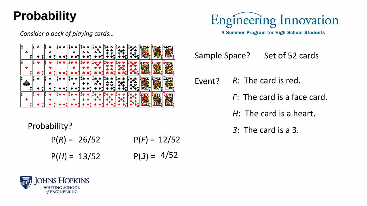
Probability
Consider a deck of playing cards…
Sample Space?
Event?
Probability?
Set of 52 cards
R: The card is red.
F: The card is a face card.
H: The card is a heart.
3: The card is a 3.P(R) = P(F) =
P(H) = P(3) =
26/52 12/52
13/52 4/52

Events and variables
Can be described as random or deterministic:
The outcome of a random event cannot be predicted:
The sum of two numbers on two rolled dice.
The time of emission of the ith particle from radioactive material.
The outcome of a deterministic event can be predicted:
The measured length of a table to the nearest cm.
Motion of macroscopic objects (projectiles, planets, space craft) as predicted by classical mechanics.

Extent of randomness
A variable can be more random or more deterministic depending on the degree to which you account for relevant parameters:
Mostly deterministic: Only a small fraction of the outcome cannot be accounted for.
Length of a table - only slightly dependent upon:
• Temperature/humidity variation• Measurement resolution• Instrument/observer error• Quantum-level intrinsic uncertainty
Mostly Random: Most of the outcome cannot be accounted for.
• Trajectory of a given molecule in a solution

Random variables
Can be described as discrete or continuous:• A discrete variable has a countable number of values.
Number of customers who enter a store before one purchases a product.
• The values of a continuous variable can not be listed:Distance between two oxygen molecules in a room.
Random Variable Possible Values
Gender Male, Female
Class Fresh, Soph, Jr, Sr
Height (inches) Integer in interval {30,90}
College Arts, Education, Engineering, etc.
Shoe Size 3, 3.5 … 18
Consider data collected for undergraduate students:
Is height a discrete or continuous variable?
How could you measure height and shoe size to make them continuous variables?

Probability Distributions
If a random event is repeated many times, it will produce a distribution of outcomes (statistical regularity).
(Think about the sum of the dots on two rolled dice)
The distribution can be represented in two ways:
• Frequency distribution function: represents the distribution as the number of occurrences of each outcome
• Probability distribution function: represents the distribution as the percentage of occurrences of each outcome

Discrete Probability Distributions
Consider a discrete random variable, X:
f(xi) is the probability distribution function
What is the range of values of f(xi)? Therefore, Pr(X=xi) = f(xi)

Discrete Probability Distributions
Properties of discrete probabilities:
0)()Pr( ii xfxX for all i
k
i
i
k
i
i xfxX11
1)()Pr( for k possible discrete outcomes
bxa
i
i
xfaFbFbXa )()()()Pr(
Where: )Pr()( xXxF
Discrete Probability Distributions
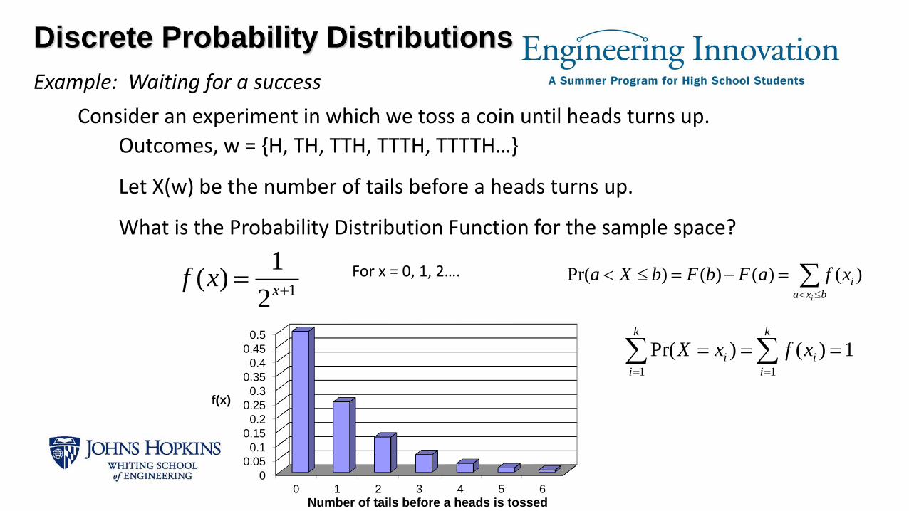
Example: Waiting for a success
Consider an experiment in which we toss a coin until heads turns up.
Outcomes, w = {H, TH, TTH, TTTH, TTTTH…}
Let X(w) be the number of tails before a heads turns up.
What is the Probability Distribution Function for the sample space?
12
1)(
xxf For x = 0, 1, 2….
0
0.05
0.1
0.15
0.2
0.25
0.3
0.35
0.4
0.45
0.5
0 1 2 3 4 5 6
f(x)
Number of tails before a heads is tossed
k
i
i
k
i
i xfxX11
1)()Pr(
bxa
i
i
xfaFbFbXa )()()()Pr(
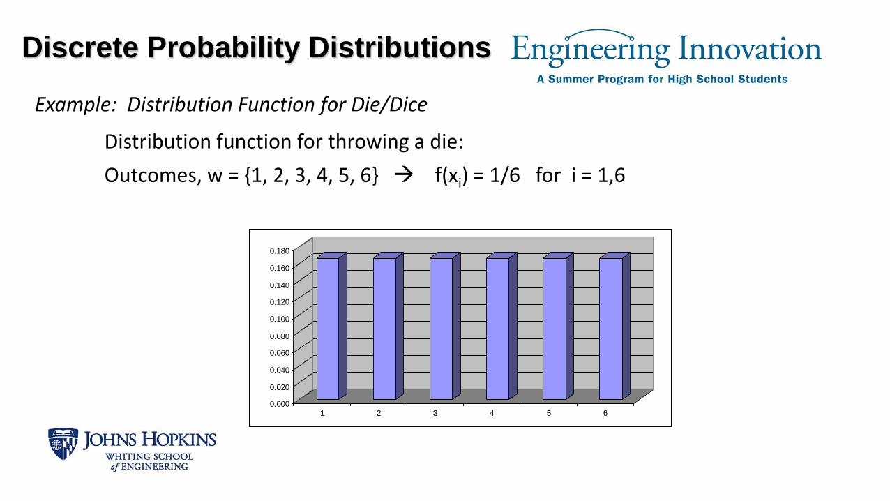
Discrete Probability Distributions
Example: Distribution Function for Die/Dice
Distribution function for throwing a die:
Outcomes, w = {1, 2, 3, 4, 5, 6} f(xi) = 1/6 for i = 1,6
0.000
0.020
0.040
0.060
0.080
0.100
0.120
0.140
0.160
0.180
1 2 3 4 5 6

Discrete Probability Distributions
Example: Distribution Function for Die/Dice
Distribution function for the sum of two thrown dice:
f(xi) = 1/36 for x1 = 2
2/36 for x2 = 3
…
0.000
0.020
0.040
0.060
0.080
0.100
0.120
0.140
0.160
0.180
2 3 4 5 6 7 8 9 10 11 12

Cumulative Discrete Probability
Distributions
j
i
ixfxFxX1
)()'()'Pr(Where xj is the largest discrete value of X less than or equal to x’
1)Pr( kxX
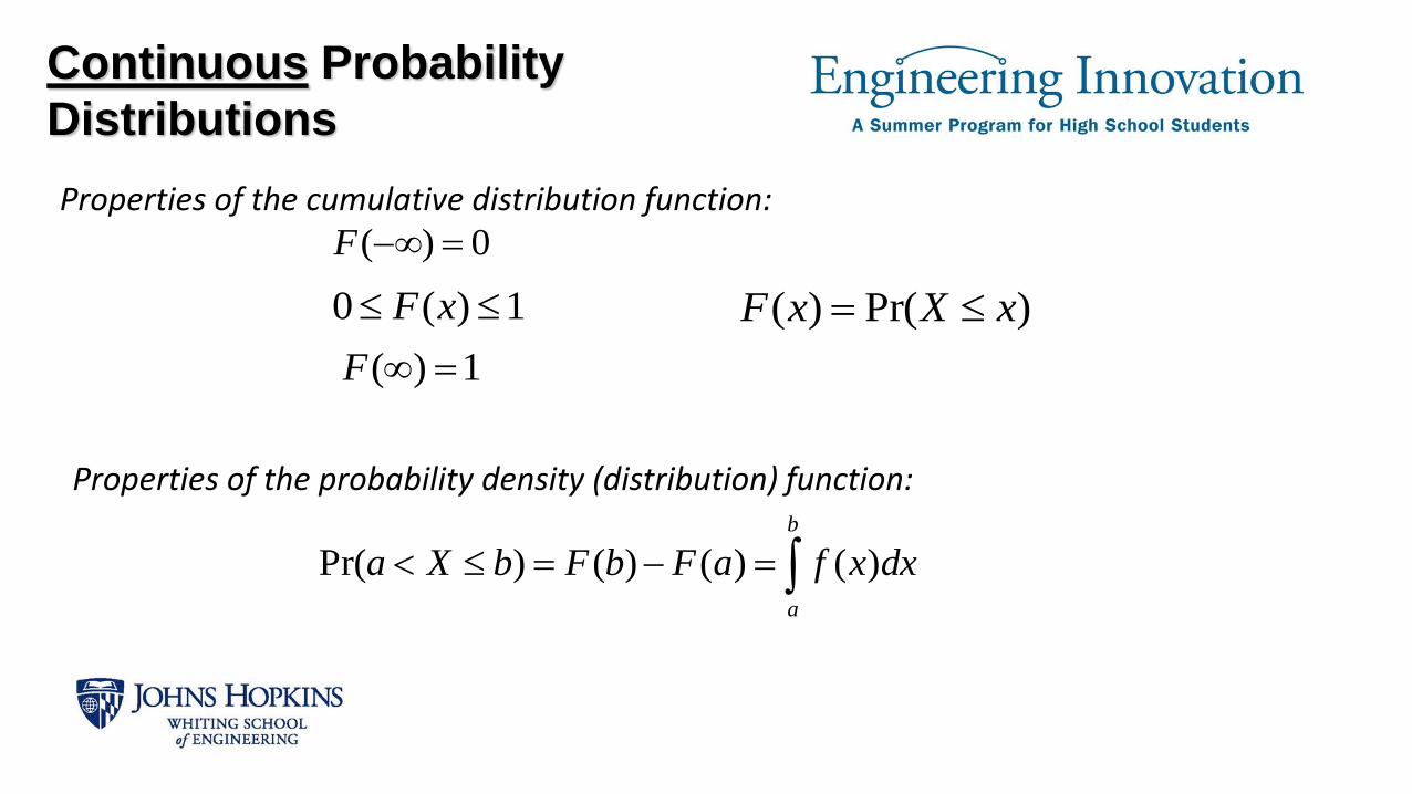
Continuous Probability
Distributions
Properties of the cumulative distribution function:
0)( F
1)(0 xF
1)( F
Properties of the probability density (distribution) function:
b
a
dxxfaFbFbXa )()()()Pr(
)Pr()( xXxF

Continuous Probability Density
FunctionCumulative Distribution Function (cdf): Gives the fraction of the total
probability that lies at or to the left of each x
Probability Density (Distribution) Function (pdf): Gives the density of concentration of probability at each point x

Continuous Probability Distributions
1
10t
F(t)
For continuous variables, the events of interest are intervals rather than isolated values.
Not interested in probability that the bus will arrive in 3.451233 minutes, but rather the probability that the bus will arrive in the subinterval (a,b) minutes:
Consider waiting time for a bus which is equally likely to arrive anytime in the next ten minutes:
10)()()(
abaFbFbTaP
Continuous Probability
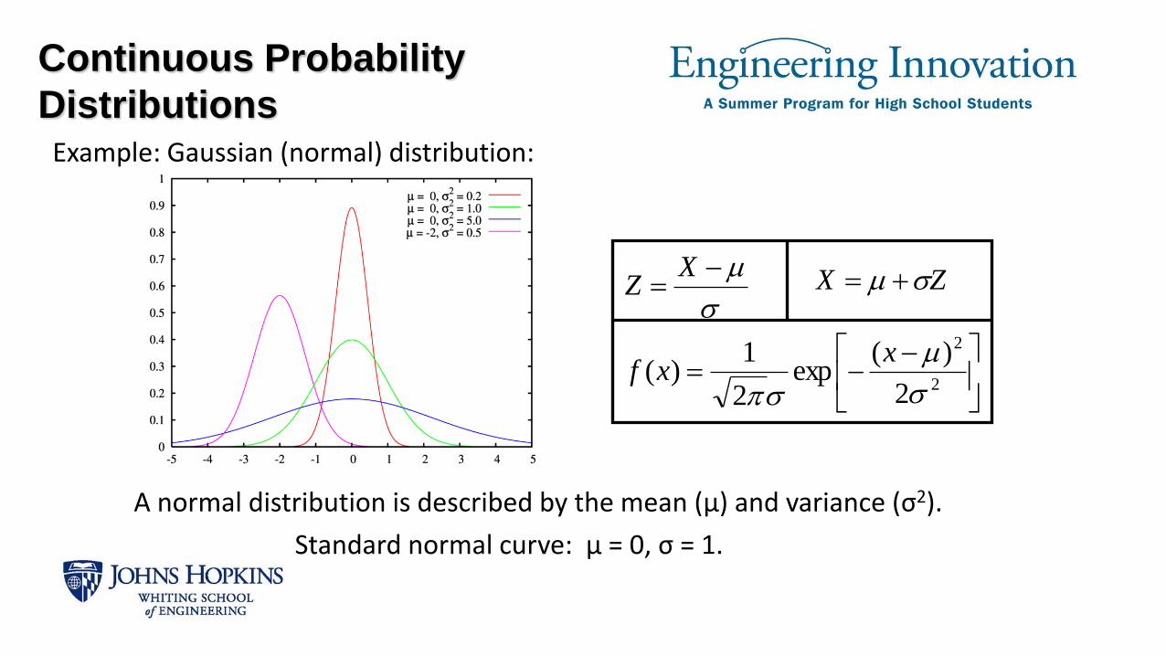
DistributionsExample: Gaussian (normal) distribution:
ZX
xxf
XZ
2
2
2
)(exp
2
1)(
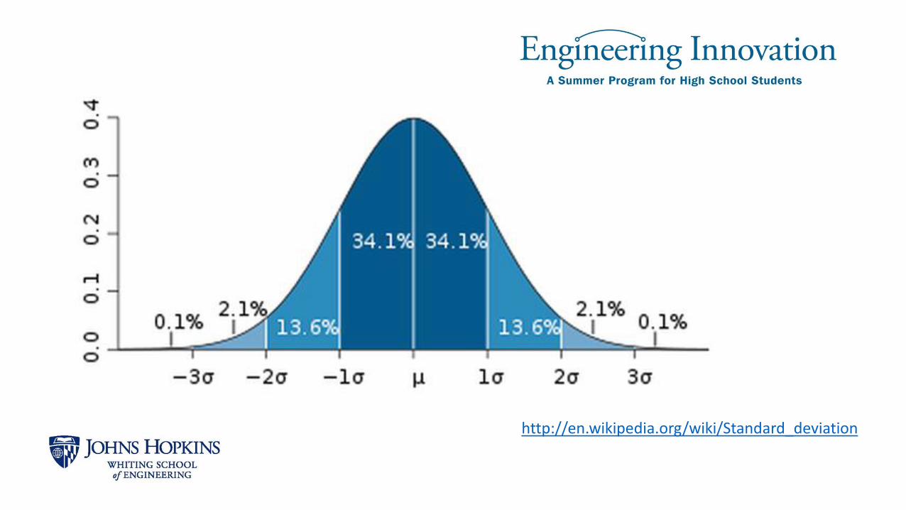
A normal distribution is described by the mean (μ) and variance (σ2).
Standard normal curve: μ = 0, σ = 1.
ZX
xxf
XZ
2
2
2
)(exp
2
1)(

Mean, Standard Deviation,
Variance
N
X
N
X
)(
)( 22
Standard Deviation:
Variance is second moment about the mean; the average squared distance of the data from the mean.
Variance:
N
X 22 )(
Standard deviation measures the spread of data about the mean.
Mean: The mean is the 1st moment about the origin; the average value of x

Two teams measure the height of a flagpole.
• Which team did the better job?
• Why do you think so?
Team A Team B
183 183.0
182 183.5
185 182.7
181 182.5
183 183.1
184 183.3
avg = avg =
183 183.0
std dev = std dev =
1.41 0.37
Height in cm
Practice!

Normal / Gaussian Distribution
Can be used to approximately describe any variable that tends to cluster around the mean.
Normal (Gaussian) Distribution:
The sum of a (sufficiently) large number of independent random variables will be approximately normally distributed.
Central Limit Theorem:
Used as a simple model for complex phenomena – statistics, natural science, social science [e.g., Observational error assumed to follow normal distribution]
Importance:
Examples of experiments/measurements that will produce Gaussian distribution?
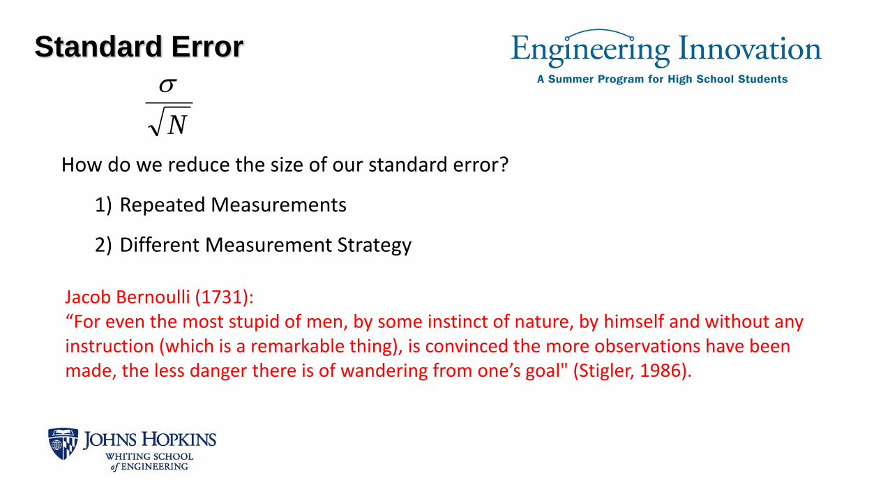
Standard Error
How do we reduce the size of our standard error?
1) Repeated Measurements
2) Different Measurement Strategy
Jacob Bernoulli (1731): “For even the most stupid of men, by some instinct of nature, by himself and without any instruction (which is a remarkable thing), is convinced the more observations have been made, the less danger there is of wandering from one’s goal" (Stigler, 1986).
N

Moments
Other values in terms of the moments:
Skewness: 2/32
3
‘lopsidedness’ of the distribution
a symmetric distribution will have a skewness = 0
negative skewness, distribution shifted to the left
positive skewness, distribution shifted to the right
Kurtosis:
Describes the shape of the distribution with respect to the height and width of the curve (‘peakedness’)
Estimation of Random Variables
Random Variable: a variable whose value is subject to variations due to chance
Assumptions/Procedures
There exists a stable underlying probability density function for the random variable
Investigating the characteristics of the random variable consists of obtaining sample outcomes and making inferences about the underlying distribution

Estimation of Random Variables
Sample statistics on a random variable X
The ith sample outcome of the variable X is denoted Xi
The sample mean : 𝑋 =1
𝑁 𝑖=1𝑁 𝑋𝑖 where N = sample size
The sample variance: 𝑠2 =1
𝑁−1 𝑖=1𝑁 𝑋𝑖 − 𝑋 2
𝑿 and s2 are estimates of the mean, , and variance, σ2, of the underlying p.d.f.
𝑋 and s2 are estimates for the sample
and σ2 are characteristics of the population from which the sample was taken
𝑋 and s2 are random variables
Expected Value, E(X)
The value that one would obtain if a very large number of samples were averaged together.
𝐸 𝑋 =
The expected value of the sample mean is the population mean
𝐸 𝑠2 = σ2
The expected value of the sample variance is the population variance
Expected values allow us to use sample statistics to infer population statistics

Properties of Expected Values
• 𝐸 𝑎𝑋 + 𝑏𝑌 = 𝑎𝐸 𝑋 + 𝑏𝐸 𝑌 where a and b are constants
• If Z = g(X), then E 𝑍 = E[g(X)] = 𝑎𝑙𝑙 𝑣𝑎𝑙𝑢𝑒𝑠 𝑥 𝑜𝑓 𝑋 𝑔 𝑥 𝑃𝑟(𝑋 = 𝑥)
Example: Throw a die. If the die shows a “6” you win $5; else, you lose a $1. What’s the expected value,E[Z], of this game?
Pr(X=1) = 1/6 g(1) = -1Pr(X=2) = 1/6 g(2) = -1Pr(X=3) = 1/6 g(3) = -1Pr(X=4) = 1/6 g(4) = -1Pr(X=5) = 1/6 g(5) = -1Pr(X=6) = 1/6 g(6) = 5
E[Z] = ([(-1)*5*1]/6)+([5*1]/6) = 0, you would not expect to win or lose

Properties of Expected Values
• 𝐸 𝑋𝑌 = 𝐸 𝑋 𝐸 𝑌 where X and Y are independent (samples of X cannot be used to predict anything about sample Y and Y cannot be used to predict X)
Example: Find the area of a picture with height, X, and width, Y.

Measurements

All measurements have errorsWhat are some sources of measurement errors?
• Instrument uncertainty (caliper vs. ruler)• Use half the smallest division (unless manufacturer provides precision information).
• Measurement error (using an instrument incorrectly)• Measure your height - not hold ruler level.
• Variations in the size of the object (spaghetti is bumpy) • Statistical uncertainty
L = 9 ± 0.5 cm
L = 8.5 ± 0.3 cm
L = 11.8 ± 0.1 cm

Estimating and Accuracy• Measurements often don’t fit the gradations of scales
• Two options:• Estimate with a single reading (take ½ the smallest division)
• Independently measure several times and take an average – try to make each trial independent of previous measurement (different ruler, different observer)
http://scidiv.bellevuecollege.edu/physics/measure&sigfigs/C-Uncert-Estimate.html
3.1 ±0.1 cm

Accuracy vs. Precision• Accuracy refers to the agreement between a measurement and the true or
accepted value• Cannot be discussed meaningfully unless the true value is known or knowable
• The true value is not usually known or may never be known)
• We generally have an estimate of the true value
• Precision refers to the repeatability of measurement• Does not require us to know the true value

http://www.shmula.com/2092/precision-accuracy-measurement-system
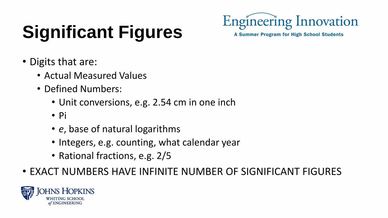
Significant Figures
• Digits that are:• Actual Measured Values
• Defined Numbers:
• Unit conversions, e.g. 2.54 cm in one inch
• Pi
• e, base of natural logarithms
• Integers, e.g. counting, what calendar year
• Rational fractions, e.g. 2/5
• EXACT NUMBERS HAVE INFINITE NUMBER OF SIGNIFICANT FIGURES
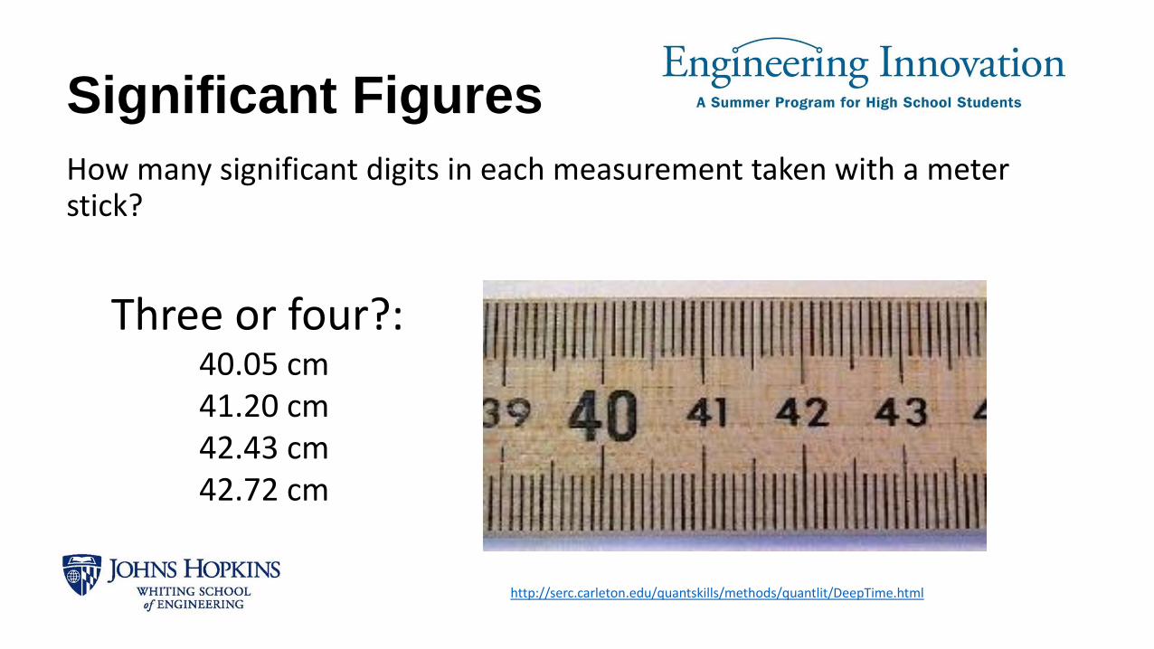
Significant Figures
How many significant digits in each measurement taken with a meter stick?
Three or four?:40.05 cm41.20 cm42.43 cm42.72 cm
http://serc.carleton.edu/quantskills/methods/quantlit/DeepTime.html

Significant Figures
• Be clear in your communication
• Which is it?
• 40 cm
• 40.0 cm
• 4 x 101 cm
http://serc.carleton.edu/quantskills/methods/quantlit/DeepTime.html

Significant Figures
• State the number of significant figures:
Value
5280
0.35
0.00307
204100
180.00
Number of significant figures
3 or 4 (unclear)
2
3
4, 5 or 6 (unclear)
5

Significant Figures
• State the number of significant figures for the number described in each phrase below:
Statement
My mattress is 182 inches long
My car gets twenty miles per gallon
5280 feet per mile
There are ten cars in that train
I am going to the Seven-Eleven
Number of significant figures
3
1 or 2
Infinite – exact number by definition
Infinite – exact number (assuming you can count to ten accurately)
0

273.92 rounded to 4 digits is
1.97 rounded to 2 digits is
2.55 rounded to 2 digits is
4.45 rounded to 2 digits is
Significant FiguresRounding:
If you do not round after a computation, you imply a greater accuracy than you actually measured
1. Determine how many digits you will keep
2. Look at the first rejected digit
3. If digit is less than 5, round down
4. If digit is more than 5, round up
5. If digit is 5, round up or down in order to leave an even number as your last significant figure
273.9
2.0
2.6
4.4
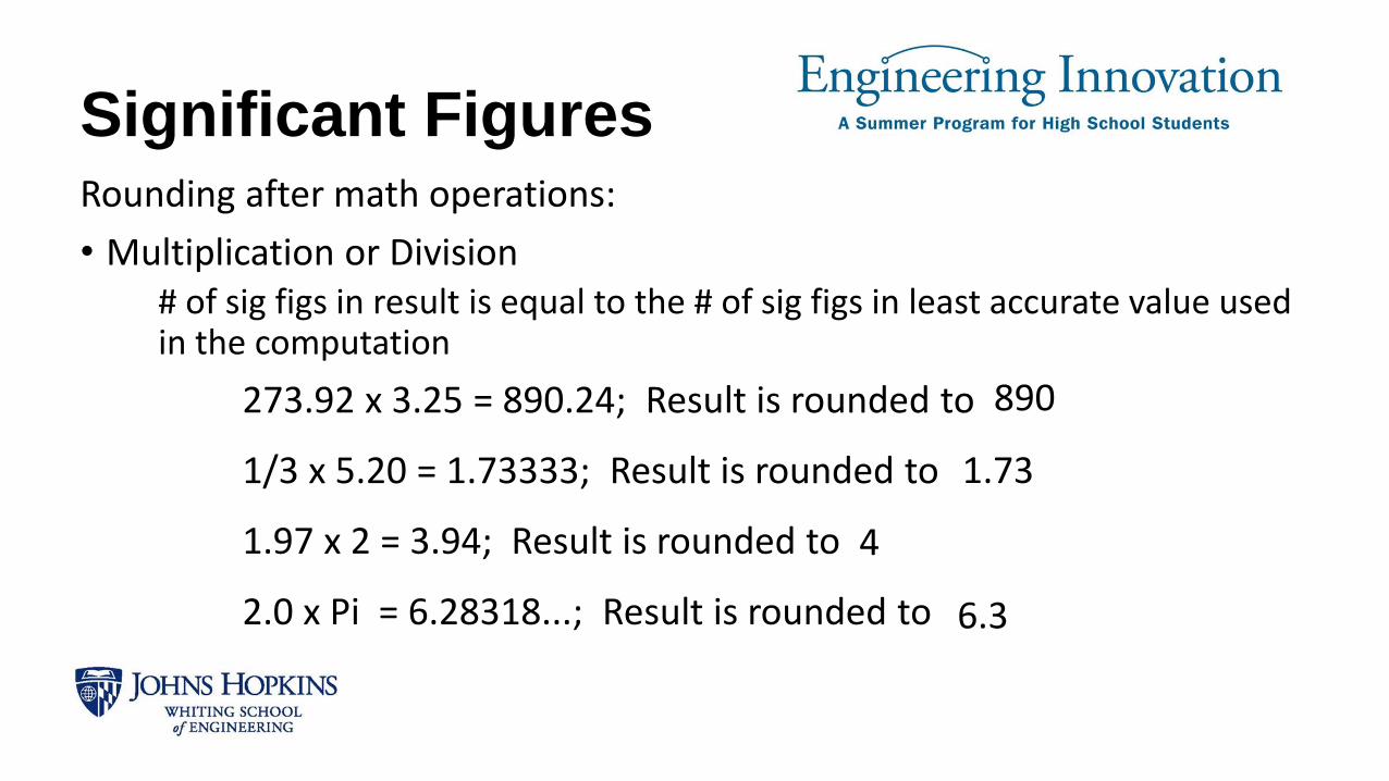
Significant FiguresRounding after math operations:
• Multiplication or Division# of sig figs in result is equal to the # of sig figs in least accurate value used in the computation
273.92 x 3.25 = 890.24; Result is rounded to
1/3 x 5.20 = 1.73333; Result is rounded to
1.97 x 2 = 3.94; Result is rounded to
2.0 x Pi = 6.28318...; Result is rounded to
890
1.73
4
6.3

Significant Figures
Rounding after math operations:
• Addition or Subtraction
Place of last sig fig is important
What’s the problem here?

Significant Figures
Multiple Calculations
• The least error will come from combining all terms algebraically, then computing all at once.
• If you need to show intermediate steps to a reader, calculate sig figs at every step. Keep an extra sig fig until the last calculation.
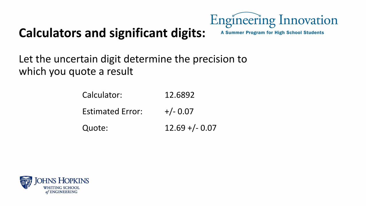
Calculators and significant digits:
Let the uncertain digit determine the precision to which you quote a result
Calculator: 12.6892
Estimated Error: +/- 0.07
Quote: 12.69 +/- 0.07

Error Analysis
What is an error?• No measurements – however carefully made- can be completely free of errors
• In data analysis, engineers use• error = uncertainty • error ≠ mistake.
• Mistakes in calculation and measurements should always be corrected before calculating experimental error.
• Measured value of x = xbest δx • xbest = best estimate or measurement of x• δx = uncertainty or error in the measurements
• Experimental uncertainties should almost always be rounded to one sig. fig
• Uncertainty in any measured quantity has the same dimensions as the measured quantity itself
• Error – difference between an observed/measured value and a true value.
• We usually don’t know the true value
• We usually do have an estimate
• Systematic Errors
• Faulty calibration, incorrect use of instrument
• User bias
• Change in conditions – e.g., temperature rise
• Random Errors
• Statistical variation
• Small errors of measurement
• Mechanical vibrations in apparatus
Error
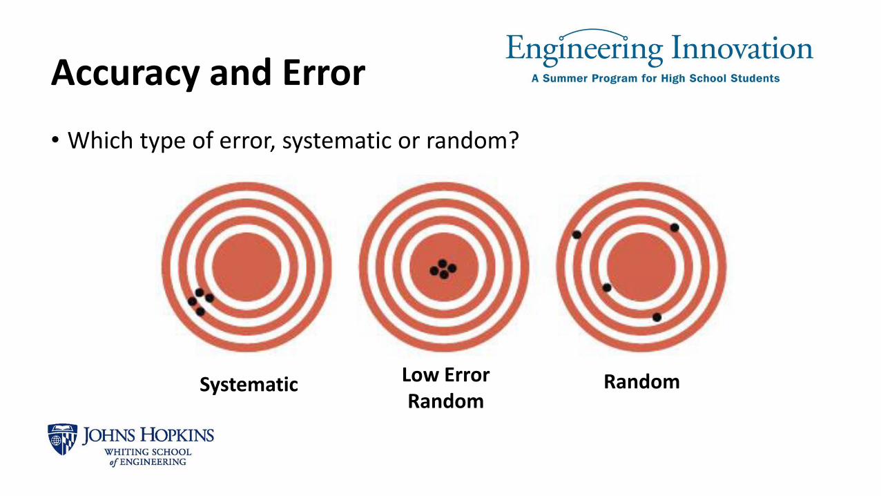
Accuracy and Error
• Which type of error, systematic or random?
Systematic Low ErrorRandom
Random

Error
• Percent Error
• Relative Error

How do you account for errors in calculations?• The way you combine errors depends on the math function
• added or subtracted –
• The sum of two lengths is Leq = L1 + L2. What is the error in Leq?
• multiplied or divide –
• The area is of a room is A = L x W. What is error in A?
• other functions (trig functions, power relationships)
• A simple error calculation gives the largest probable error.

Sum or difference • What is the error if you add or subtract numbers?
• The absolute error is the sum of the absolute errors.
xx yy zz
zyxw
boundupper zyxw

What is the error in length of molding to put around a room?
• L1 = 5.0cm 0.5cm and L2 = 6.0cm 0.3cm.
• The perimeter is
• The error (upper bound) is:
cm22
cm0.6cm0.5cm0.6cm0.5
2121
LLLLL
cm6.1
cm3.0cm5.0cm3.0cm5.0
2121
LLLLL
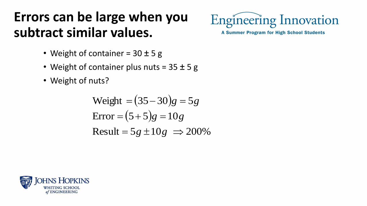
Errors can be large when you subtract similar values.
• Weight of container = 30 ± 5 g
• Weight of container plus nuts = 35 ± 5 g
• Weight of nuts?
%200105Result
1055Error
53035Weight
gg
gg
gg

Product or quotient
• What is error if you multiply or divide?
• The relative error is the sum of the relative errors.
z
yxw
boundupper z
z
y
y
x
x
w
w
xx yy zz
zz
yyxxw
)()(
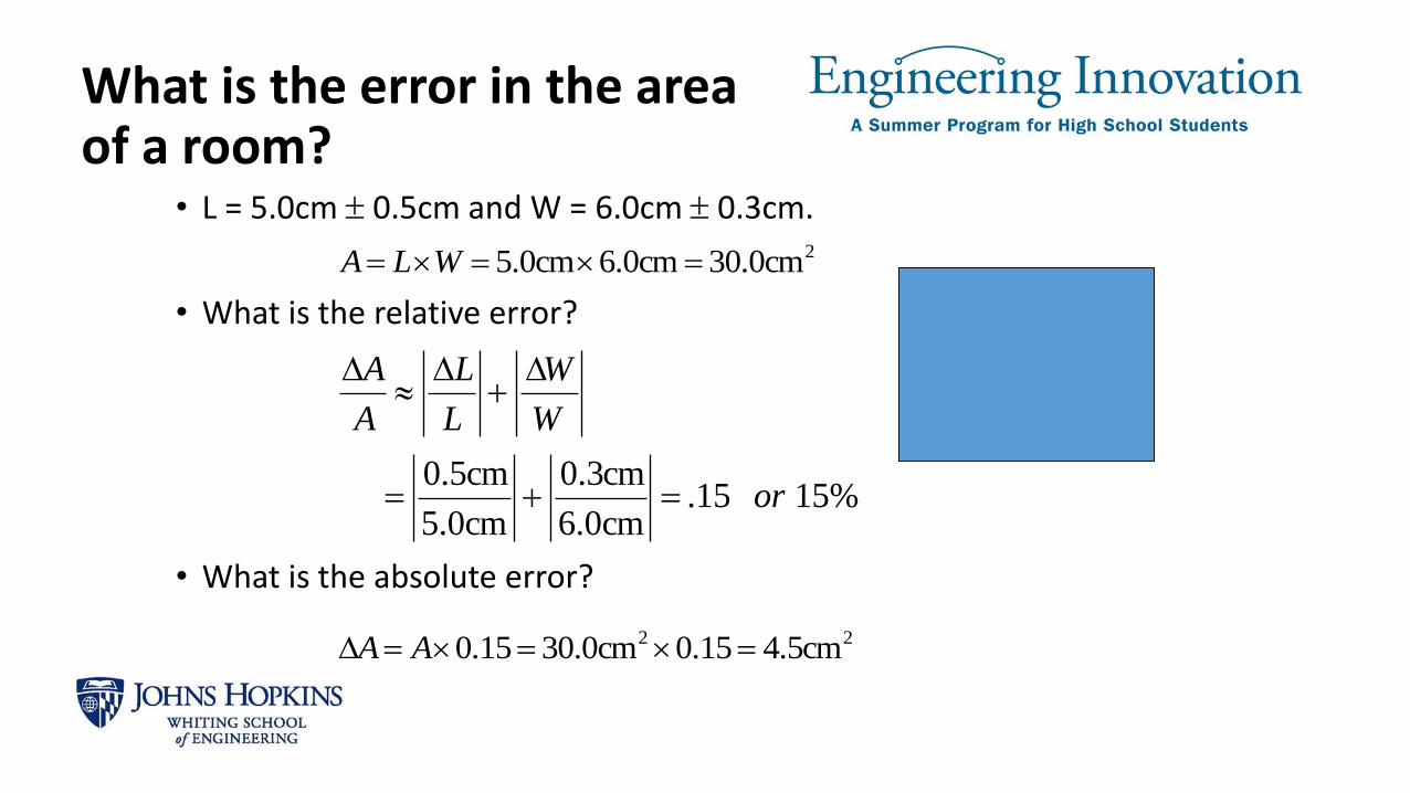
What is the error in the area of a room?
• L = 5.0cm 0.5cm and W = 6.0cm 0.3cm.
• What is the relative error?
• What is the absolute error?
2cm0.30cm0.6cm0.5 WLA
%1515.cm0.6
cm3.0
cm0.5
cm5.0
or
W
W
L
L
A
A
22 cm5.415.0cm0.3015.0 AA

Multiply by constant
• What if you multiply a variable x by a constant B?
• The error is the constant times the absolute error.
Bxw
xBw

What is the error in the circumference of a circle?
• C = 2 π R
• For R = 2.15 ± 0.08 cm
• C = 2 π (0.08 cm)
= 0.50 cm
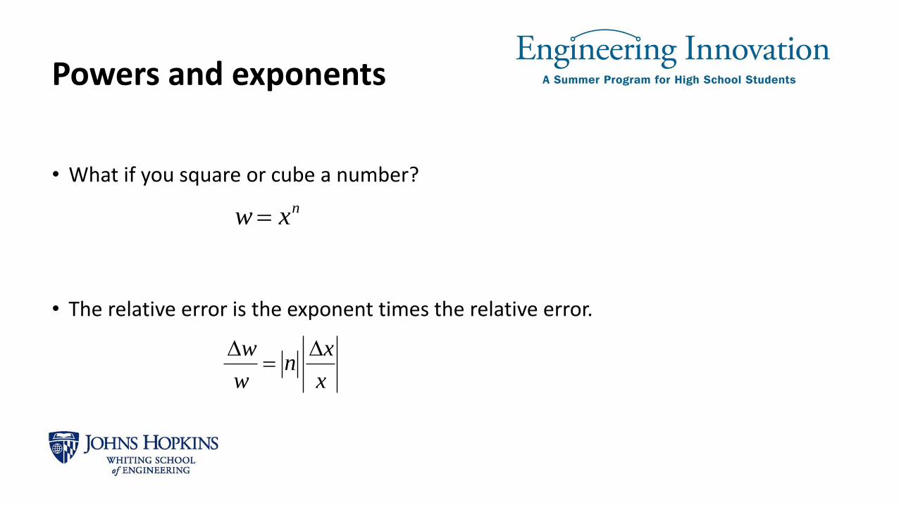
Powers and exponents
• What if you square or cube a number?
• The relative error is the exponent times the relative error.
nxw
x
xn
w
w
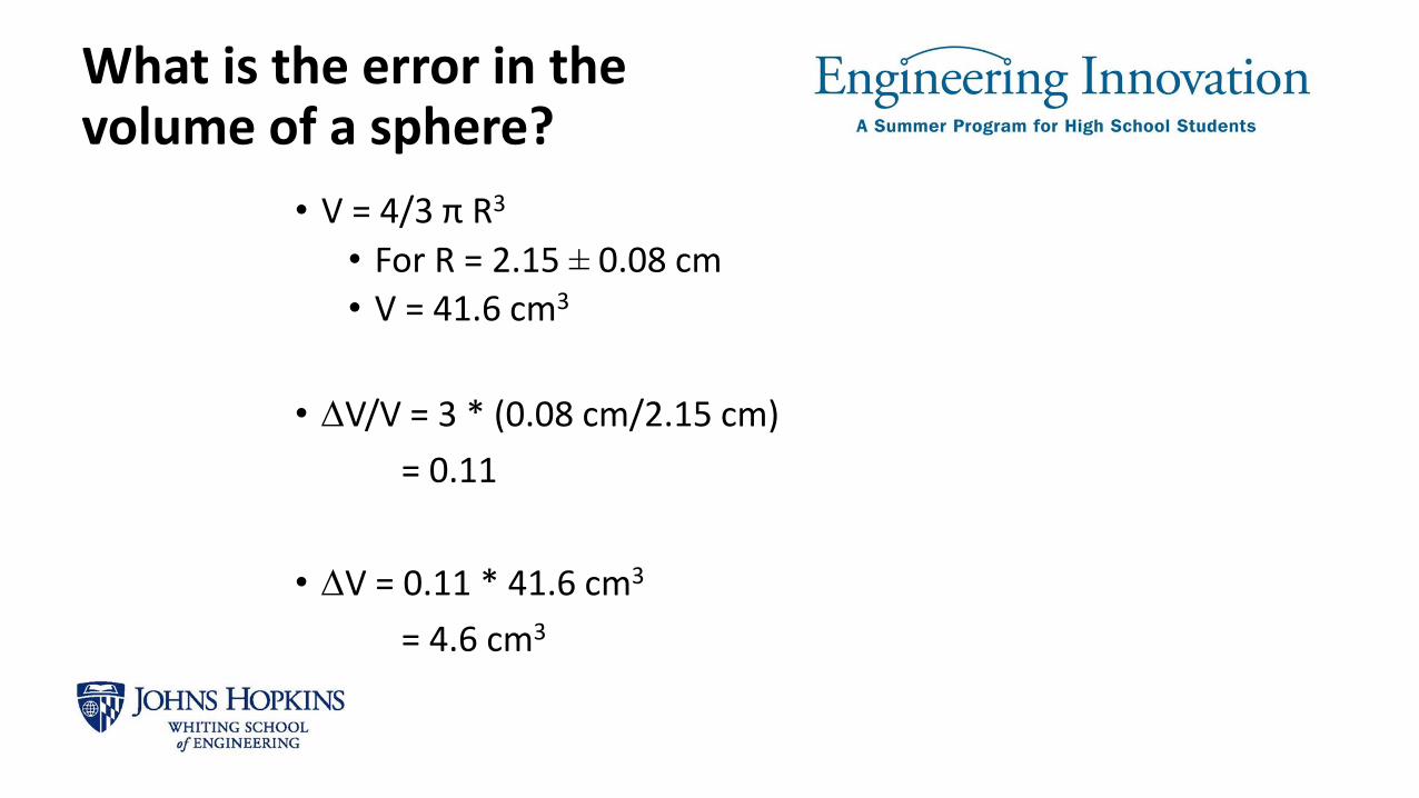
What is the error in the volume of a sphere?
• V = 4/3 π R3
• For R = 2.15 ± 0.08 cm
• V = 41.6 cm3
• V/V = 3 * (0.08 cm/2.15 cm)
= 0.11
• V = 0.11 * 41.6 cm3
= 4.6 cm3

Trig Functions
• What if you are using a trigonometric function?
)sin()sin(
)sin(
xxxw
xw

Remote Measurement Lab “Calculus of Errors” Explanation