p. 1

Uncertainty Analysis of Climate Change and Policy Response

Mort Webster1, Chris Forest2, John Reilly2, Mustafa Babiker3, David Kicklighter4, Monika Mayer5, Ronald Prinn2, Marcus Sarofim2, Andrei Sokolov2, Peter Stone2,

Chien Wang2

1Department of Public Policy, University of North Carolina Chapel Hill, CB# 3435, Chapel Hill, NC, 27599;

2MIT Joint Program on the Science and Policy of Global Change, 1 Amherst St., E40-271, Massachusetts Institute of Technology, Cambridge, MA 02139;

3Arab Planning Institute, P.O. Box 5834, Safat 13059, KUWAIT; 4Ecosystems Center at Marine Biological Laborartory, 7 MBL Street, Woods Hole, MA 02543;

5AVL List GmbH, Hans List Platz 1, A-8020 GRAZ, Austria

Abstract

To aid climate policy decisions, accurate quantitative descriptions of the

uncertainty in climate outcomes under various possible policies are needed. Here, we

apply an earth systems model to describe the uncertainty in climate projections under two

different policy scenarios. This study illustrates an internally consistent uncertainty

analysis of one climate assessment modeling framework, propagating uncertainties in

both economic and climate components, and constraining climate parameter uncertainties

based on observation. We find that in the absence of greenhouse gas emissions

restrictions, there is a one in forty chance that global mean surface temperature change

will exceed 4.9oC by the year 2100. A policy case with aggressive emissions reductions

over time lowers the temperature change to a one in forty chance of exceeding 3.2oC,

thus reducing but not eliminating the chance of substantial warming.

p. 2

1. Introduction

Policy formulation for climate change poses a great challenge because it presents

a problem of decision-making under uncertainty (Manne and Richels, 1995; Morgan and

Keith, 1995; Nordhaus, 1994; Webster, 2002; Hammit et al., 1992). While continued

basic research on the climate system to reduce uncertainties is essential, policy-makers

also need a way to assess the possible consequences of different decisions, including

taking no action, within the context of known uncertainties. Here, we use an earth

systems model to describe the uncertainty in climate projections under two different

policy scenarios related to greenhouse gas emissions. This analysis propagates

uncertainties in emissions projections and uses observations to constrain uncertain

climate parameters. We find that with a policy of no restrictions on greenhouse gas

(GHG) emissions, there is one chance in two that the increase in global mean temperature

change over the next century will exceed 2.4oC and one chance in twenty that it will be

outside the range 1.0-4.9oC. A second hypothetical policy case with aggressive

emissions reductions over time lowers the temperature change to one chance in two of

exceeding 1.6oC and one chance in twenty of being outside the range 0.8-3.2oC; thus this

policy reduces the chance of high levels of global warming but does not eliminate the

chance of substantial warming.

Decision-making under uncertainty is an appropriate framework for the climate

problem because of two basic premises: (i) the cumulative nature of atmospheric

greenhouse gases, and the inertia of the oceans, means that if one waits to resolve the

amount of climate change in 2050 or 2100 by perfectly observing (or forecasting) it, it

will take decades or centuries to alter the observed trends—effective mitigation action

p. 3

must be started decades before the climate changes of concern are actually observed; (ii)

a significant part of our uncertainty about future climate change may be unavoidable—

details of climate and weather over longer periods are likely to remain unpredictable to

some degree, and uncertainty in projecting future levels of human activities and

technological change is inevitable. Thus, informed climate policy decisions require

current estimates of the uncertainty in consequences for a range of possible actions.

Furthermore, the use of consistent and well-documented methods to develop these

uncertainty estimates will allow us to track the changes in our understanding through

time.

Recognition of the importance of providing uncertainty estimates has been

increasing in recent years. Authors for the Third Assessment Report (TAR) of the

Intergovernmental Panel on Climate Change (IPCC) were encouraged to quantify

uncertainty as much as possible (Moss and Schneider, 2000) and indeed, uncertainty was

quantified for some aspects of climate change in the TAR. Uncertainty in key results,

however, such as the increase in global mean surface temperature through 2100, was

given only as a range without probabilities (Houghton et al., 2001). Since the IPCC TAR

was published, several studies have recognized this shortcoming and contributed

estimates of the uncertainty in future climate change (Schneider, 2001; Allen et al., 2001;

Wigley and Raper, 2001; Knutti et al., 2002; Stott and Kettleborough, 2002).

These previous attempts to describe uncertainty have, however, been limited in

significant ways. First, recent climate observations were not used to constrain the

uncertainty in climate model parameters in some studies (Wigley and Raper, 2001).

Second, by using only one Atmosphere-Ocean General Circulation Model (AOGCM),

p. 4

uncertainties in climate model response are reduced to uncertainty in a single scaling

factor for optimizing the model’s agreement with observations (Stott and Kettleborough,

2002). Third, the IPCC’s emissions scenarios were not intended to be treated as equally

likely, yet some authors have assumed that they were (Wigley and Raper, 2001). Indeed,

Schneider (2001, 2002) has demonstrated the ambiguity and potential dangers that result

from the absence of probabilities assigned to emissions scenarios. Fourth, other authors

estimated uncertainty in future climate change only applied to specific IPCC emissions

scenarios rather than providing equal treatment of the uncertainty in the emissions

projections (Allen et al., 2001; Knutti, et al., 2002; Stott and Kettleborough, 2002). As

such, these studies analyzed the uncertainty only in the climate system response without

characterizing the economic uncertainty except through individual IPCC emissions

scenarios. Finally, none of these previous studies have examined the uncertainty in

future climate change under a policy scenario leading to stabilization of GHG

concentrations.

Our study builds on previous estimates of uncertainty in future climate changes

but with three significant improvements: (1) we use explicit probabilities for different

emissions projections, based on judgments about the uncertainty in future economic

growth and technological change (Webster et al., 2002) and on documented uncertainty

in current levels of emissions (Olivier et al., 1995); (2) we use observations to constrain

the joint distributions of uncertain climate parameters so that simulated climate change

for the 21st century is consistent with observations of surface, upper-air, and deep ocean

temperatures over the 20th century (Forest et al., 2000, 2001, 2002); and (3), we estimate

uncertainty under a policy constraint as well as a no policy case, to show how much

p. 5

uncertainty remains even after a relatively certain cap on emissions is put in place. Using

this approach, we provide a more comprehensive picture of the relative likelihood of

different future climates than previously available.

The no policy and policy constraint cases are modeled as once-and-for-all

decisions, with no learning or change in policy along the way. In reality, climate policy

will be revised as we continue to learn and respond to new information and events.

Policy decisions are therefore better modeled as sequential decisions under uncertainty

(Webster, 2002; Hammitt et al., 1992; Manne and Richels, 1995). In order to perform

such analyses, however, the uncertainty in projections must first be quantified. Thus the

work presented here is a necessary precursor to a more sophisticated treatment of climate

policy. Also, we present here an analysis of uncertainty in one modeling framework,

which does not treat all of the structural uncertainties.

The quantification of probabilities for emissions forecasts has been the topic of

some debate. There are two distinct ways to approach the problem of forecasting when

there is substantial uncertainty: uncertainty analysis (associating probabilities with

outcomes), and scenario analysis (developing “plausible” scenarios that span an

interesting range of possible outcomes). The IPCC Special Report on Emissions

Scenarios (SRES) (Nakicenovic, 2000) used the plausible scenario approach, where all

the scenarios developed were considered “equally valid” without an assignment of

quantitative or qualitative likelihoods.

One benefit of a scenario approach is that it allows detailed exploration of what

outcomes are produced by particular sets of assumptions. In assessments involving a set

p. 6

of authors with widely diverging views, it is typically easier to avoid an impasse by

presenting equally valid scenarios without attaching likelihoods.

Uncertainty analysis requires identification of the critical uncertain model

structures and parameters (or inputs), quantification of the uncertainty in those structures

and parameters in the form of probability distributions, and then sampling from those

distributions and performing model simulations repeatedly to construct probability

distributions of the outcomes. With this approach, one can quantify the likelihood that an

outcome of a model (or range of models) falls within some specified range. Hence, unlike

the scenario approach, uncertainty analyses indicate better the likelihood of the potential

consequences, or risks, of a particular policy decision.

It has been argued that when it comes to socio-economic processes that drive

emissions, there should be no attempt to assign probabilities. However, if emissions

projections are presented without relative likelihoods, non-experts will substitute their

own judgment (Schneider, 2001). One analysis has assumed that all of the IPCC SRES

scenarios were equally likely (Wigley and Raper, 2001). Other studies have used one or

two representative scenarios to calculate future uncertainty (Allen et al., 2001; Knutti, et

al., 2002; Stott and Kettleborough, 2002), which then require judgments about the

likelihood of the emissions scenarios that were used if they are to be relevant to policy.

By using formal techniques to elicit judgments from those who are expert in the

underlying processes that contribute to uncertainty in future emissions, one can provide

this additional information for policymaking.

Because judgments are ultimately required for policy decisions, the difference

between formal quantitative uncertainty analysis and the scenario approach is not

p. 7

whether a judgment about likelihood of outcomes is needed but rather when and by

whom the judgment is made. The evidence is strong that experts and non-experts are

equally prone to well-known cognitive biases when it comes to assigning probabilities,

but also that formal quantitative approaches can reduce these biases (Morgan and

Henrion, 1990; Tversky and Kahneman, 1974). Thus, unless scientists who develop

future climate projections use the tools of uncertainty analysis and their judgment to

describe the likelihood of outcomes quantitatively, the assessment of likelihood will be

left to other scientists, or policy makers, or the public who will not have all the relevant

information behind those projections (Moss and Schneider, 2000). Our views are that:

(1) experts should offer their judgment about uncertainty in their projections, and (2)

formal uncertainty techniques can eliminate some of the cognitive biases that exist when

people deal with uncertainty. Of course, there will remain a need for experts and non-

experts to make judgments about uncertainty results: uncertainty analysis is an important

contributor to policy making but it may be no easier to achieve expert consensus for a

particular distribution of outcomes than it is to achieve consensus about a point estimate.

Further, model-based quantitative uncertainty analysis cannot easily account for

uncertainty in processes that are so poorly understood that they are not well represented

in the models. For example, there is considerable evidence that there can be abrupt

collapses in the ocean's thermohaline circulation (e.g., Higgins et al., 2002.) No coupled

GCM has yet shown such an abrupt change on the time scale that we have considered, up

to 2100, but the fact that these same models give very diverse projections for changes in

the thermohaline circulation (Cubasch et al, 2001) is evidence that our ability to model

these processes is poor. Thus, similar to many other assessment models, our modeling

p. 8

framework presented below does not currently reproduce many of the abrupt state

changes discussed in Higgins et al (2002). Such abrupt changes could certainly affect the

probability distribution of outcomes if they could be included (see e.g., distributions from

experts no. 2 and 4 in the elicitation by Morgan and Keith, 1995). As the state of the art

in models and representation of these mechanisms improves, their effects should be

included in uncertainty analyses.

2. Methods

We specifically consider uncertainty in: 1) anthropogenic emissions of

greenhouse gases [carbon dioxide (CO2), methane (CH4), nitrous oxide (N2O),

hydrofluorocarbons (HFCs), perfluorocarbons (PFCs) and sulfur hexafluoride (SF6)]; 2)

anthropogenic emissions of short-lived climate-relevant air pollutants [sulfur dioxide

(SO2), nitrogen oxides (NOx), carbon monoxide (CO), ammonia (NH3), black carbon

(BC), organic carbon (OC), and non-methane volatile organic compounds (NMVOCs)];

3) climate sensitivity (S); 4) oceanic heat uptake as measured by an effective vertical

ocean diffusivity (Kv); and 5) specific aerosol forcing (Faer).

We constrain uncertainty in climate model parameters to be consistent with

climate observations over much of the past century (Forest et al., 2002), and we use

uncertainty estimates in anthropogenic emissions (Webster et al., 2002) for all relevant

greenhouse gases (GHGs) and aerosol and GHG precursors as estimated using the MIT

Emissions Prediction and Policy Analysis (EPPA) model (Babiker et al., 2000, 2001).

These results (Webster et al., 2002; Forest et al., 2002) provide input distributions that we

use for the earth systems components of the MIT Integrated Global System Model

p. 9

(IGSM) (Prinn et al., 1999; Reilly et al., 1999), an earth system model of intermediate

complexity (Claussen, 2002). The MIT IGSM has been developed specifically to study

uncertainty quantitatively. It achieves this by retaining the necessary complexity to

adequately represent the feedbacks and interactions among earth systems and the

flexibility to represent the varying parameterizations of climate consistent with the

historical data. At the same time, it remains computationally efficient so that it is

possible to make hundreds of multi-century simulations in the course of a few months

with a dedicated parallel processing computer system. Using efficient sampling

techniques, Latin Hypercube sampling (Iman and Helton, 1998), a sample size of 250 is

sufficient to estimate probability distributions for climate outcomes of interest.

2.1 STRUCTURE OF THE MIT IGSM

The MIT IGSM components include: (a) the EPPA model, designed to project

emissions of climate-relevant gases and the economic consequences of policies to limit

them (Babiker et al., 2000, 2001), (b) the climate model, a two-dimensional (2D) zonally-

averaged land-ocean (LO) resolving atmospheric model, coupled to an atmospheric

chemistry model, (c) a 2D ocean model consisting of a surface mixed layer with specified

meridional heat transport, diffusion of temperature anomalies into the deep ocean, an

ocean carbon component, and a thermodynamic sea-ice model (Sokolov and Stone, 1998;

Wang et al., 1998, 1999; Holian et al., 2001), (d) the Terrestrial Ecosystem Model (TEM

4.1) (Melillo et al., 1993; Tian et al., 1999), designed to simulate carbon and nitrogen

dynamics of terrestrial ecosystems, and (e) the Natural Emissions Model (NEM) that

p. 10

calculates natural terrestrial fluxes of CH4 and N2O from soils and wetlands (Prinn et al.,

1999; Liu, 1996).

The version of the MIT IGSM used here contains certain other unique and

important features. It incorporates a computationally efficient reduced-form urban air

chemistry model derived from an urban-scale air pollution model (Mayer et al., 2000).

Also, TEM is now fully coupled with the 2D-LO ocean-atmosphere-chemistry model1.

In previous simulations (Prinn et al., 1999; Reilly et al., 1999), an iterative coupling

procedure was performed to include the effect of climate change on the carbon uptake by

land ecosystems. The new fully integrated version includes direct monthly interaction

between the climate and ecosystem components: the 2D-LO climate model provides

monthly averaged temperature, precipitation, and cloud cover and TEM returns the

carbon uptake or release from land for the month. The coupling of the zonally averaged

2D-LO climate model to a latitude-longitude grid to drive TEM requires scaling the

present-day longitudinal distribution of climate data by the projected zonally averaged

quantities, which has been shown to work well as compared with input from three-

dimensional models (Xiao et al., 1997).

A simple representation of sea level change due to melting of mountain glaciers

has been incorporated into the IGSM. Change in the volume of glaciers from year t0 to

year t (expressed as the equivalent (expressed as the equivalent volume of liquid water) is

calculated as

dttTgdTgdBBotSgdV

t

to

))()(( ∆+= ∫ ,

p. 11

where B0 is the rate of increase in global sea level due to melting of glaciers in the

year t0, dTgdB is the sensitivity of this rate of increase to changes in global average

annual mean surface temperature, Tg, and Sg is the total glacial area. Sg in a year t is

calculated as,

)1()1()( −+−= tdSgtSgtSg ,

dSg is assumed to be proportional to dV. Change in sea level is computed using the total

ocean surface area Ao as,

AodVdh = .

In all our calculations we use year 1990 as t0. Values of B0 and dTgdB , 0.4 mm/year

and 0.61 mm/year/degree respectively, were derived from the published results of

transient climate change simulations with a number of coupled atmosphere-ocean GCMs

(Church et al, 2001). The differences in these parameters as simulated by the different

models were small compared to the uncertainty in projections of changes in Tg associated

with other uncertainties, such as climate sensitivity. Thus by taking fixed values of these

parameters, we are assuming that the major uncertainty in dV is due to the uncertainty in

dTg. This approach is a simplified version of that used by Gregory and Oerlemans

(1998).

1 Anthropogenic emissions of greenhouse gases from human activities are treated parametrically in the EPPA model. A version of the ecosystems model that includes human-induced land-use change, including a mechanistic model of GHG emissions from land use is being developed for future versions of the IGSM.

p. 12

2.2 UNCERTAINTY IN IGSM CLIMATE PARAMETERS

The century-scale response of the climate system to changes in the radiative

forcing is primarily controlled by two uncertain global properties of the climate system:

the climate sensitivity and the rate of oceanic heat uptake (Sokolov and Stone, 1998;

Sokolov et al., 2002). In coupled Atmosphere-Ocean General Circulation Models

(AOGCMs) these two essentially structural properties are determined by a large number

of equations and parameters and cannot easily be changed. The sensitivity, S, of the MIT

climate model, however, can be easily varied by changing the strength of the cloud

feedback (i.e., we can mimic structural differences in the AOGCMs). Mixing of heat into

the deep ocean is parameterized in the MIT model by an effective diffusion applied to a

temperature difference from values in a present-day climate simulation. Therefore, the

rate of the oceanic heat uptake is defined by the value of the globally averaged diffusion

coefficient, Kv. By varying these two parameters the MIT climate model can reproduce

the global-scale zonal-mean responses of different AOGCMs (Sokolov and Stone, 1998).

Because of this flexibility our results for these responses are not as model dependent as

they would be if we had used a single AOGCM for all of our analysis. There is also

significant uncertainty in the historical forcing mainly associated with uncertainty in the

radiative forcing in response to a given aerosol loading, Faer17. Thus, in the MIT IGSM,

these three parameters (S, Kv, and Faer) are used to characterize both the response of the

climate system and the uncertainty in the historical climate forcing.

A particularly crucial aspect of our uncertainty work was estimating the joint pdfs

for the climate model parameters controlling S, Kv, and Faer. Previous work has used pdfs

based on expert judgment or results from a set of climate models (Hammit et al., 1992;

p. 13

Wigley and Raper, 2001; Titus and Narayan, 1995; Webster and Sokolov, 2000). Our

method uses observations of upper air, surface, and deep-ocean temperatures for the 20th

century to jointly constrain these climate parameters, while including natural climate

variability as a source of uncertainty (Forest et al., 2002). The method for estimating pdfs

relies on estimating goodness-of-fit statistics, r2 (Forest et al., 2000, 2001, 2002),

obtained from an optimal fingerprint detection algorithm (Allen and Tett, 1999).

Differences in r2 provide a statistic that can be used in hypothesis testing, and thereby

provide probability estimates for parameter combinations (Forest et al., 2000, 2001). We

compute r2 by taking the difference in the modeled and observed patterns of climate

change and weighting the difference by the inverse of the natural variability for the

pattern. This method requires an estimate of the natural variability (i.e., unforced) for the

climate system over very long periods. Ideally, observed climate variability would be

used but reconstructed data are not of sufficient accuracy. Our estimate was obtained

from long control runs of particular AOGCMs (Forest et al., 2002). Estimates of the

variability from other AOGCMs could change the results.

Starting with a prior pdf over the model parameter space, an estimate of the

posterior pdf is obtained by applying Bayes Theorem (Bayes, 1763), using each

diagnostic to estimate a likelihood function, and then each posterior becomes the prior for

the procedure using the next diagnostic. In the work presented here, expert priors for

both S and Kv were used (Webster and Sokolov, 2000), but sensitivity to alternative

assumptions will be presented2. Fractiles for the final posterior distributions used here for

the climate model parameters are shown in Table 1. The three diagnostics are treated as

p. 14

independent observations and, therefore, weighted equally in the Bayesian updating

procedure.

The result is a joint pdf for these three parameters with correlation among the

marginal pdfs (e.g., a high climate sensitivity is only consistent with observed

temperature under some combination of rapid heat uptake by the ocean and a strong

aerosol cooling effect). The pairwise correlation coefficients are 0.243 for S-Faer, 0.093

for Kv-Faer, and 0.004 for S-Kv,

2.3 SPIN-UP OF CLIMATE MODEL IN MONTE CARLO EXPERIMENTS

A further issue in the Monte Carlo analysis is the so-called “spin-up” of the IGSM

components required with different sampled values of changes in S, Kv, and Faer. There is

inertia in the ocean and carbon cycle models, as well as TEM, so that one cannot start

“cold” from the year 2000 with different values for climate parameters. The

computational requirements for running the full model starting from pre-industrial times

through 2100 for each of the 250 runs necessitated a two-stage spin-up procedure. For

the first stage, a simulation of the IGSM in spin-up mode was carried out with reference

values for S, Kv, and Faer for the period Jan. 1, 1860 to Jan. 1, 1927. In this mode, the

climate model uses estimated historical forcings while the ocean carbon-cycle model

(OCM) and TEM are forced by observed changes in CO2 concentrations and the climate

variables as simulated by the climate model. Carbon uptake by the OCM and TEM are

not fed back to the climate model in this stage. The model states in 1927 for the climate

model and TEM from this run were saved and then used as initial conditions for the

2 There is debate over whether and how to combine subjective probability distributions from multiple experts for use in an uncertainty analysis; see, e.g., Titus and Narayanan (1996), Pate-Cornell (1996), Keith

p. 15

second spin-up stage with the different sets of model parameters sampled in the Monte

Carlo analysis. During this second stage the IGSM was run in the same mode as the first

stage from Jan. 1, 1927 to Jan. 1, 1977, but using the different sampled values for the

climate parameters. Given the inertia in the OCM, that model component was run from

1860 in all simulations and the required climate data up to 1927 were taken from the

climate simulation for reference parameter values. Test runs of the full IGSM spun-up

from 1860 using extreme values of the uncertain parameters were compared with results

from this shortened spin-up procedure and showed no noticeable difference in the

simulation results by 1977, confirming that this shortened spin-up period would not affect

projections of future climate.

The full version of the IGSM was then run beginning from Jan. 1, 1977 using

historical anthropogenic emissions of GHGs and other pollutants through 1997 and

predicted emissions for 1998 through 2100. During this stage of the simulations all

IGSM components are fully interactive: carbon uptake by the OCM and TEM are used in

the atmospheric chemistry model and soil carbon changes simulated by TEM are used in

NEM. Concentrations of all gases and aerosols as well as associated radiative forcings

are calculated endogenously. The atmospheric chemistry model and NEM components

use the same initial conditions for 1977 in all simulations. Short-lived species do not

require a long spin-up period because they have relatively little inertia, while the long-

lived species, including CO2, N2O, CH4, and CFCs, have been prescribed during spin-up

and are restricted to observations over 1977-1997.

The 1977 to 1997 period provides additional information on the consistency of the

ocean and terrestrial carbon uptake. Given data on anthropogenic emissions and actual

(1996), and Genest and Zidek (1986).

p. 16

atmospheric concentrations, total carbon uptake by the ocean and terrestrial systems can

be estimated to have averaged 4.3 TgC/year during the 1980s. Carbon uptake by the

ocean strongly depends on the values of climate parameters, especially Kv. Across the

250 runs, the implied distribution for oceanic carbon uptake averaged over the 1980s has

a mean of 2.1 TgC/year with 95 percent bounds of 0.9 and 3.2 TgC/year. This

distribution is quite similar to results from a more complete treatment of uncertainty in

the OCM (Holian et al., 2001). Because we do not treat uncertainty in TEM for this

study, carbon uptake by the terrestrial eco-system shows too little variance. Thus for

every sample parameter set, we calculate an additional sink/source needed to balance the

carbon cycle for the decade 1980-1989, and retain this sink/source as a constant addition

for each individual through the year 2100.

During the spin-up phase, as described in Forest et al. (2001), aerosol forcing is

parameterized by a change in surface albedo and depends on historical SO2 emissions and

a scattering coefficient that sets the forcing level in response to the prescribed aerosol

loading. In each simulation, this coefficient is used to set the sampled value of Faer. In the

period beyond 1977 using the full version of the IGSM, the sampled value of Faer is now

a function of the aerosol optical depth multiplier and the initial SO2 emission. Based on

the results of preliminary simulations, the following formula was obtained for the aerosol

optical depth multiplier Cf (see Table 6 in Forest et al., 2001):

Cf=A*Faer(1+x)/E(1+y),

where E is the global SO2 emissions, x=0.035 and y=0.0391 and the value of A was

defined from a reference simulation. The dependence on the initial SO2 emissions

reflects uncertainty in the present day aerosol loading. We use the aerosol optical depth

p. 17

multiplier to provide the sampled value of Faer. Thus, the choice of parameters in each

period of the simulation ensures a smooth transition in the net forcing between different

stages of the run as well as consistency with the historical climate record.

2.4 DATA FOR PARAMETER DISTRIBUTIONS

The critical input data for uncertainty analyses are the probability distribution

functions (pdfs) for the uncertain parameters. A key error frequently made in assembling

such pdfs is to use the distribution of point estimates drawn from the literature rather than

from estimates of uncertainty (e.g., standard deviation) itself. Examples of such errors

are estimates of future emissions uncertainty based on literature surveys of emissions

projections, or estimates of uncertainty in climate sensitivity based on their distribution

from existing climate models. There is nothing inherently wrong with using literature

estimates, but the point estimates of uncertain parameters should span the population of

interest and not simply a distribution of mean estimates from different studies.

There can be a variety of problems with using literature estimates. For example,

the distribution of emissions scenarios based on a literature review showed maximum

probability at the level of one of the central emissions scenarios produced by the second

assessment report of the IPCC (Houghton et al., 1996). However, subsequent evaluation

of the same literature (Nakicenovic et al., 1998) indicates that many analysts simply

adopted this scenario as a convenient reference to conduct a policy study, rather than to

conduct a new and independent forecast of emissions. The frequent reappearance of this

estimate in the literature should not be interpreted as indicating a particular judgment that

the scenario was much more likely than others. Similarly, the fact that the IPCC scenarios

p. 18

span the range in the literature provides no evidence of whether they describe uncertainty

in future emissions, although recent analyses (Wigley and Raper, 2001) have attempted to

interpret them as such. Basing the distribution of climate sensitivity on the distribution of

estimates from a set of climate models makes a similar mistake. There is no reason to

expect that the climate sensitivities in this set of models provide an unbiased estimate of

either the mean or the variance, because some models are simply slight variants, or use

parameterizations similar to those in other models. But, just because one parent model

has given rise to more models does not mean that the sensitivities of this group of models

should be weighted more than another model—more versions does not make it more

likely to be correct. The goal is to perform internally-consistent uncertainty analysis to

understand the likelihood of different outcomes.

2.5 ANTHROPOGENIC EMISSIONS PROBABILITY DENSITY FUNCTIONS

Uncertainties in anthropogenic emissions were determined using a Monte Carlo

analysis of the MIT EPPA model, which is a computable general equilibrium model of

the world economy with sectoral and regional detail (Babiker et al., 2000, 2001). As

emissions projections for all substances are derived from a single economic model, the

projections are self-consistent with the economic activity projections. The correlation

structure among emissions forecasts reflects the structure of the model. Specifically,

because energy production and agriculture are simultaneous sources of many GHGs and

air pollutants, there is a strong correlation among emissions of the various gases and

aerosols (Webster et al., 2002). An approach that used different models for different sets

of emissions might erroneously treat the distributions of emissions as independent. We

p. 19

used an efficient and accurate method for sampling the input parameter space to produce

a reduced form (response surface) model (Tatang et al., 1997) of the underlying EPPA

model. A full Monte Carlo analysis is then conducted using the response surface model.

Based on sensitivity analysis of the EPPA model, a limited set of EPPA input

parameters was identified for uncertainty treatment. These were: labor productivity

growth; autonomous energy efficiency improvement (AEEI); factors for emissions per

unit of economic activity for agricultural and industrial sources of CH4 and N2O; factors

for emissions per unit of economic activity in fossil fuel, agricultural and industrial

sources of SO2, NOx, CO, NMVOC, BC, OC, and NH3; and emissions growth trends for

HFCs, PFCs, and SF6. The underlying distributions were based on a combination of

expert elicitation of the distributions (labor productivity and AEEI), on estimates of

uncertainty in emission coefficients from the literature (i.e., not a distribution of point

estimates), and statistical analysis of cross-section dependence of emissions per unit of

economic activity on per capita income. Thus, we account for the uncertainty in today’s

global emissions, as well as the uncertainty in how quickly different economies around

the globe will reduce pollutants as their wealth increases. Many derivative factors

traditionally treated as uncertain parameters, such as energy prices, introduction of new

technologies, sectoral growth, and resource exhaustion, are endogenously calculated in

EPPA. The projections of these economic processes (and thus emissions from different

activities) are uncertain but that uncertainty derives from the more fundamental

uncertainty in productivity growth and energy efficiency and from the structure of the

model.

p. 20

2.6 LATIN HYPERCUBE SAMPLING UNCERTAINTY ANALYSIS

Sampling from the probability distributions for the uncertainty analysis is

performed using Latin Hypercube Sampling (LHS) (Iman and Helton, 1988). LHS

divides each parameter distribution into n segments of equal probability, where n is the

number of samples to be generated. Sampling without replacement is performed so that

with n samples every segment is used once. Samples for the climate parameters are

generated from the marginal pdfs, and the correlation structure among the three climate

model parameters is imposed (Iman and Conover, 1982). This ensures that the low

probability combinations of parameters are not over-represented, as would be the case if

the correlations were neglected.

We conducted two LHS uncertainty analyses for the period 1860-2100, in both

cases using n = 250. One analysis included uncertainty in climate variables and

emissions in the absence of policy. The second analysis restricted the emissions path for

greenhouse gases, by assuming a policy constraint. The policy scenario chosen was one

used in previous work (Reilly et al., 1999), which comes close to a 550 ppm stabilization

case for reference climate model parameter values. It assumes that the Kyoto Protocol

caps are implemented in 2010 in all countries that agreed to caps in the original protocol

(i.e., including the United States even though the US has indicated it will not ratify the

protocol) (United Nations, 1997). The policy scenario also assumes that the Kyoto

emissions cap is further lowered by 5 percent every 15 years so that by 2100 emissions of

all greenhouse gases in all countries under the original Kyoto cap are 35 percent below

1990 levels. With regard to countries not capped by the Kyoto Protocol, the policy

scenario assumes that they take on a cap in 2025 with emissions 5 percent below their

p. 21

(unconstrained) 2010 emissions levels. The cap is then reduced by 5 percent every 15

years thereafter so that these countries are 30 percent below their 2010 emissions by

2100. Because we assume no uncertainty in these caps, the emissions uncertainty is

greatly reduced. Some emissions uncertainty remains, however, because there is no cap

on any nation until 2010 and the cap for the developing countries is started even later and

depends on their uncertain 2010 emissions. This cap is only applied to CO2, and does not

explicitly constrain other greenhouse gases or air pollutants, but because of the

correlation between sources captured in the structure of the model, there will be some

corresponding reduction in these other emissions as well.

3. Results and Discussion

3.1 ANALYSIS OF UNCERTAINTY WITH AND WITHOUT POLICY

In the absence of any climate policy, we find that the 95% bounds on annual CO2

emissions by 2100 are 7 to 38 GtCyr-1 with a mean of 19 GtCyr-1. This range is similar to

that of the six SRES marker scenarios. However by explicitly providing the probability

distribution, we reduce the chances that someone would incorrectly assume that scenarios

resulting in 7 and 38 GtCyr-1 are equally likely as those that result in 19 GtCyr-1.

The biggest difference between our emissions distributions and the SRES

(Nakicenovic et al., 2000) scenarios are for SO2 projections. First, unlike the IPCC

analysis, we consider the uncertainty in current annual global emissions, which is

substantial: 95% bounds of 20 to 105 TgSyr-1 with a mean of 58 TgSyr-1 in 1995 (Olivier

et al., 1995; Van Aardenne et al., 2001). Secondly, we consider the uncertainty in future

SO2 emissions controls. In all six of the SRES marker scenarios reported in the IPCC

p. 22

TAR, SO2 emissions begin to steadily decline after about 2040. Thus, all these SRES

scenarios assume that policies will be implemented to reduce sulfur emissions, even in

developing countries, for all imaginable futures. In contrast, our study assumes that the

ability or willingness to implement sulfur emissions reduction policies is one of the key

uncertainties in these projections. Accordingly, our 95% probability range by 2100, 20 to

230 TgSyr-1 with a mean of 100 TgSyr-1, includes the possibility of continuing increases

in SO2 emissions over the next century, or of declining emissions consistent with SRES.

Neither extreme is considered as likely as a level similar to today’s emissions. A large

part of our uncertainty in SO2 emissions can be traced to the fact that we are uncertain

about current emissions. While there are many inventories of emissions by governments

that purport to track emissions of pollutants, the apparent accuracy suggested by them

does not reflect the underlying problems in measurement or lack of comprehensive

measurement of all sources. Thus emissions estimates often cannot be easily and

accurately reconciled with observed pollutant levels. In considering emissions

uncertainty, in contrast to the SRES approach, it is therefore essential to evaluate

uncertainty in current emissions where that is important as well as in factors that affect

growth in emissions.

The stringent policy causes the median CO2 concentration in 2100 to be nearly

200 ppm lower (Figure 1A), the median radiative forcing to be about 2.5 Wm-2 lower

(Figure 1B), and the global mean temperature to be about 1.0oC lower (Figure 1C) than in

the no policy case. The policy reduces the 95% upper bound for the increase in

temperature change by 2oC (from 4.9oC to 3.2oC).

p. 23

We estimate probability distributions (Figure 2) for global mean temperature

change, sea level rise, and carbon uptake by the terrestrial biosphere. For each model

output, the cumulative distribution (CDF) of the 250 results is fit to an analytical

distribution that minimizes the squared differences between the empirical and analytical

CDFs. The comparison between the empirical and analytical distributions is shown only

for temperature change in 2100 with no policy (Figure 2A) to illustrate the approximate

nature of the fits and the caution needed in evaluating small probability regions (e.g., the

tails of the distribution). Without policy, our estimated mean for the global mean surface

temperature increase is 1.1˚C in 2050 and 2.4˚C in 2100. The corresponding means for

the policy case are 0.93˚C in 2050 and 1.7˚C in 2100. The mean outcomes tend to be

somewhat higher than the modes of the distribution, reflecting the skewed distribution—

the mean outcome of the Monte Carlo analysis is higher than if one were to run a single

scenario with mean estimates from all the distributions. One can also contrast the

distribution for the no policy case with the IPCC range for 2100 of 1.4 to 5.8˚C

(Houghton et al., 2001). Although the IPCC provided no estimate of the probability of

this range, our 95 percent probability range for 2100 is 1.0 to 4.9˚C. So, while the width

of the IPCC range turns out to be very similar to our estimate of a 95 percent confidence

limit, both their lower and upper bounds are somewhat higher. When compared to our

no-policy case, our policy case produces a narrower pdf and lower mean value for the

1990-2100 warming (Figure 2B). But, even with the reduced emissions uncertainty in the

policy case, the climate outcomes are still quite uncertain. There remains a one in forty

chance that temperatures in 2100 could be greater than 3.2˚C and a one in seven chance

that temperatures could rise by more than 2.4˚C, which is the mean of our no policy case.

p. 24

Hence, climate policies can reduce the risks of large increases in global temperature, but

they cannot eliminate the risk.

We also report uncertainty in sea level rise due to thermal expansion of the ocean

and melting of glacial ice (Figure 2C). These two processes are expected to be the

primary sources of sea level rise over the next century3, and the policy reduces the 95%

upper bound for sea level rise by 21 cm (from 84 cm to 63 cm)4. Finally, the uptake of

carbon into the terrestrial biosphere (Figure 2D) is much more uncertain and has higher

mean values in the no policy case than in the policy case, due to the larger and continual

increases in atmospheric CO2 concentrations in the no policy case (Figure 1A).

As changes in surface temperature will not be uniform across the surface of the

earth, it is useful to examine the dependence of projected temperatures on latitude (Figure

3). As in all current AOGCMs, the warming at high latitudes, as well as the uncertainty

associated with this warming, is significantly greater than in the tropics, and the 95%

upper bound warming with no policy is quite substantial in the high latitudes: there is a

one in forty chance that warming will exceed 8oC in the southern high latitudes and 12oC

in the north.

3 We exclude contributions from the Greenland and Antarctic ice sheets, but most studies indicate these would have a negligible contribution in the next century (IPCC 2001; Bugnion, 2000). 4 For cases of stabilization such as these, one observes about 70% of equilibrium warming by the time stabilization occurs, and the remaining 30% would be realized gradually over the next 200 to 500 years. Sea level rise takes even longer to equilibrate: at the time of stabilization one sees only about 10% of the ultimate equilibrium rise, with the remaining 90% occurring over the next 500 to 1000 years. Climate

p. 25

3.2 ROBUSTNESS OF RESULTS

To test the robustness of the results, we propagated a second set of probability

distributions for the uncertain climate parameters. Instead of beginning with prior pdfs

from expert judgment and using the observation-based diagnostics to constrain the pdfs,

we begin with uniform priors (i.e., equal likelihood over all parameter values) and then

constrain based on observations. This results in a joint pdf with greater variance, and is

the pdf described in Forest et al. (2002). The resulting uncertainty in temperature change

by 2100 is somewhat greater: the 95% probability bounds are 0.8o to 5.5oC (Figure 4A).

A larger increase in uncertainty is seen in sea level rise due to thermal expansion: the

upper 95% bound increases from 83 cm to 87 cm and the probability that sea level rise

will exceed 50 cm by 2100 increases from 32% to 49% (Figure 4B). This is largely due

to the inability of the climate change diagnostics to constrain the uncertainty in rapid heat

uptake by the deep ocean (Forest et al., 2002).

3.3 COMPARISON TO OTHER APPROACHES

Using results from model comparisons to describe uncertainty will tend to

underestimate the variance in climate outcomes. As an illustration, we compare the

transient climate response (TCR), which is defined as the change in global mean

temperature at the time of CO2 concentration doubling with a 1%yr-1 increase in CO2

atmospheric concentrations, for the models given in Table 9.1 of the TAR (Cubasch et al,

2001) to the pdf of the TCR from the MIT IGSM (Figure 5). The pdf for the MIT model

is calculated by propagating the distributions for climate sensitivity and heat uptake by

‘equilibrium’ is, itself, a troublesome concept as there is natural variation in climate that takes place on many different time scales. And, stabilization is at best an approximate concept (Jacoby et al., 1996).

p. 26

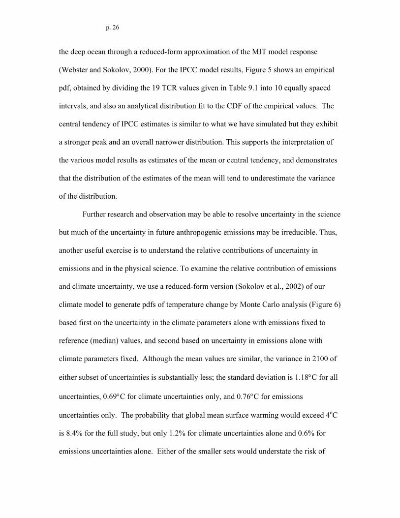
the deep ocean through a reduced-form approximation of the MIT model response

(Webster and Sokolov, 2000). For the IPCC model results, Figure 5 shows an empirical

pdf, obtained by dividing the 19 TCR values given in Table 9.1 into 10 equally spaced

intervals, and also an analytical distribution fit to the CDF of the empirical values. The

central tendency of IPCC estimates is similar to what we have simulated but they exhibit

a stronger peak and an overall narrower distribution. This supports the interpretation of

the various model results as estimates of the mean or central tendency, and demonstrates

that the distribution of the estimates of the mean will tend to underestimate the variance

of the distribution.

Further research and observation may be able to resolve uncertainty in the science

but much of the uncertainty in future anthropogenic emissions may be irreducible. Thus,

another useful exercise is to understand the relative contributions of uncertainty in

emissions and in the physical science. To examine the relative contribution of emissions

and climate uncertainty, we use a reduced-form version (Sokolov et al., 2002) of our

climate model to generate pdfs of temperature change by Monte Carlo analysis (Figure 6)

based first on the uncertainty in the climate parameters alone with emissions fixed to

reference (median) values, and second based on uncertainty in emissions alone with

climate parameters fixed. Although the mean values are similar, the variance in 2100 of

either subset of uncertainties is substantially less; the standard deviation is 1.18°C for all

uncertainties, 0.69°C for climate uncertainties only, and 0.76°C for emissions

uncertainties only. The probability that global mean surface warming would exceed 4oC

is 8.4% for the full study, but only 1.2% for climate uncertainties alone and 0.6% for

emissions uncertainties alone. Either of the smaller sets would understate the risk of

p. 27

extreme warming as we understand the science of climate change today. If it were

possible to significantly resolve climate science over the next few years, about one-third

of the uncertainty, as measured by the standard deviation, could be reduced. Reducing

the odds of serious climate change thus requires both improved scientific research and

policies that control emissions.

Because the climate model parameters can be chosen such that the model

reproduces the global scale zonal-mean transient results of a particular AOGCM

(Sokolov et al., 2002), we can repeat the above experiment choosing parameter settings

corresponding to specific AOGCMs. Three such cases, for GFDL_R15, HadCM3, and

NCAR CSM, have been chosen because they represent a wide range of climate change

results simulated by AOGCMs (Sokolov et al., 2002). To simulate such results, we first

derive the conditional pdf of aerosol forcing from our constrained joint pdf of climate

parameters, conditioned on the values of S and Kv that match the IGSM to a particular

model (Figure 7A). We then draw 250 Latin Hypercube samples from the conditional

aerosol pdf and use the original 250 samples of all emissions parameters. Finally,

because of computation time considerations, we perform the Monte Carlo on a reduced-

form model fit to the IGSM. The reduced-form model is a 3rd-order response surface fit

based on the 500 runs of the IGSM (presented above) and has an R2 of 0.97.

The simulated pdfs for surface warming 1990-2100 from these models (Figure

7B) indicate that any single AOGCM will have less variance in temperature change than

a complete treatment of the uncertainty, not surprisingly, considering that the sensitivity

and heat uptake are fixed. The mean estimates of temperature change for the models are

ordered as one would expect given the climate parameter values that allow us to

p. 28

reproduce them with the MIT IGSM. In particular, the HadCM3 and GFDL models have

a higher mean for their distribution of temperature change than the NCAR model, with

the NCAR mean near the mean of the full distribution but with smaller variance.

4. Conclusions

The Third Assessment Report of the Intergovernmental Panel on Climate Change

strove to quantify the uncertainties in the reported findings, but was limited in what could

be said for future climate projections given the lack of published estimates. This study is

a contribution to help fill that gap in the literature, providing probability distributions of

future climate projections based on current uncertainty in underlying scientific and

socioeconomic parameters, and for two possible policies over time. In reality, there will

be the possibility to adapt climate policy over time as, through research and observation,

we learn which outcomes are more likely. But decisions today can only be based on the

information we have today. The work presented here is one attempt to bring together

current knowledge on science and economics to understand the likelihood of future

climate outcomes as we understand the science and economics today. A necessary part

of the research on climate change is to repeat this type of analysis as our understanding

improves so that we can better understand the policy relevance of these scientific

advances.

As with all investigations of complex and only partially understood systems, the

results presented here must be treated with appropriate caution. Current knowledge of

the stability of the great ice sheets, stability of thermohaline circulation, ecosystem

transition dynamics, climate-severe storm connections, future technological innovation,

p. 29

human population dynamics, and political change, among other relevant processes, is

limited. Therefore abrupt-changes or “surprises” not currently evident from model

studies, including our uncertainty studies summarized here, may occur.

While our approach allows us to simulate climate responses over a range of

different structural assumptions in 3D models, other structural features of our modeling

system are fixed for this analysis even though alternative assumptions are also possible.

We hope that uncertainty studies of other climate models will soon follow, making use of

ever-increasing processor speeds, efficient sampling techniques, and reduced-form

models to make uncertainty analyses feasible on even larger models that require more

computational time.

Acknowledgements

We thank Myles Allen for his assistance and support with the detection

diagnostics. We also thank Steve Schneider and four anonymous reviewers for helpful

comments and suggestions. This research was conducted within the Joint Program on the

Science and Policy of Global Change with the support of a government-industry

partnership that includes the Integrated Assessment program, Biological and

Environmental Research (BER), U.S. Department of Energy (DE-FG02-94ER61937), the

Methane Branch of the US EPA (grant X-827703-01-0), NSF grant ATM-9523616,

Methods and Models for Integrated Assessment Program of the NSF (DEB-9711626),

and a group of corporate sponsors from the United States, the European Community, and

Japan.

Correspondance and requests should be addressed to M.Webster (email: mort@unc.edu).

p. 30

Refererences

Allen, M. et al.: 2002, Surveys in Geophysics, in press.

Allen, M. R. and Tett, S.F.B.: 1999, Clim. Dyn. 15, 419-434.

Babiker, M. et al.: 2001, ‘The MIT Emissions Prediction and Policy Analysis (EPPA)

Model: Revisions, Sensitivities, and Comparison of Results’, Report No. 71, Joint

Program on the Science and Policy of Global Change, MIT, Cambridge, MA. Or

see http://web.mit.edu/globalchange/www/MITJPSPGC_Rpt71.pdf

Babiker, M., Reilly, J. and Ellerman, D.: 2000, ‘Japanese Nuclear Power and the Kyoto

Agreement’, Journal of Japanese and International Economies 14, 169-188.

Bayes, T.: 1763, Phil. Trans. Royal Society 53, 370-418.

Bugnion, V. 2000, ‘Reducing the uncertainty in the contributions of Greenland to Sea-

level rise in the 20th and 21st centuries’, Annals of Glaciology 31, 121-125.

Church, J. A., Gregory, J. M. et al.: 2001, “Changes in Sea Level”, Chapter 11 in Climate

Change 2001: The Scientific Basis, Contribution of Working Group I to the

Second Assessment Report of the Intergovernmental Panel on Climate Change,

Houghton, J.T., Ding, Y., Griggs, D.J., Noguer, M., van der Linden, P.J., Dai, X.,

Maskell, K., and Johnson, C.A. (eds.), Cambridge University Press, Cambridge

and New York.

Claussen, M. et al.: 2002, ‘Earth system models of intermediate complexity: Closing the

gap in the spectrum of climate system models’, Climate Dyn., 18, 579-586.

Cubasch, U., Meehl, G. A. et al.: 2001, “Projections of Future Climate Change”, Chapter

9 in Climate Change 2001: The Scientific Basis, Contribution of Working Group I

p. 31

to the Second Assessment Report of the Intergovernmental Panel on Climate

Change, Houghton, J.T., Ding, Y., Griggs, D.J., Noguer, M., van der Linden, P.J.,

Dai, X., Maskell, K., and Johnson, C.A. (eds.), Cambridge University Press,

Cambridge and New York.

Forest, C. E., Stone, P. H., Sokolov, A. P., Allen, M. R. and Webster, M. D.: 2002,

‘Quantifying Uncertainties in Climate System Properties with the Use of Recent

Climate Observations’, Science 295, 113-117.

Forest, C. E., Allen, M. R., Sokolov, A. P. and Stone, P. H.: 2001, ‘Constraining Climate

Model Properties Using Optimal Fingerprint Detection Methods’, Clim. Dyn. 18,

227-295.

Forest, C. E., Allen, M. R., Stone, P. H., and Sokolov, A. P.: 2000, ‘Constraining

Uncertainties in Climate Models Using Climate Change Detection Techniques’,

Geophys. Res. Let. 24(4), 569-572.

Genest, C. and Zidek, J. V.: 1986, ‘Combining Probability Distributions: a Critique and

Annotated Bibliography’, Statistical Science 1, 114-148.

Gregory, J. M. and Oerlemans J.: 1998, ‘Simulated future sea-level rise due to glacier

malt based on regionally and seasonally resolved temperature changes’, Nature

391, 474-476.

Hammit, J. K., Lempert, R. J. and Schlesinger, M. E.: 1992, ‘A Sequential-Decision

Strategy for Abating Climate Change’, Nature 357, 315-18.

Holian, G., Sokolov, A.P. and Prinn, R.G.: 2001, ‘Uncertainty in Atmospheric CO2

Predictions from a Parametric Uncertainty Analysis of a Global Ocean Carbon

p. 32

Cycle Model’, Report No. 80, Joint Program on the Science and Policy of Global

Change, MIT, Cambridge, MA, 2001. Or see

http://web.mit.edu/globalchange/www/MITJPSPGC_Rpt80.pdf

Houghton, J.T., Meira Filho, L.G., Callander, B.A., Harris, N., Kattenberg, A., and

Maskell, K. (eds.): 1996, Climate Change 1995—The Science of Climate Change,

Contribution of Working Group I to the Second Assessment Report of the

Intergovernmental Panel on Climate Change, Cambridge University Press,

Cambridge and New York.

Iman, R. L. and Helton, J. C.: 1998, ‘An Investigation of Uncertainty and Sensitivity

Analysis Techniques for Computer Models’, Risk Analysis 8(1), 71-90.

Iman, R. L. and Conover, W. J.: 1982, ‘A Distribution-Free Approach to Inducing Rank

Correlation Among Input Variables’, Communications in Statistics B11(3), 311-

334.

Jacoby, H.D., Schmalensee, R. and Reiner, D.M.:1996, ‘What Does Stabilizing

Greenhouse Gas Concentrations Mean?’ in Flannery, B., Kolhase, K. and

LeVine, D. (eds.), Critical Issues in the Economics of Climate Change,

International Petroleum Industry Environmental Conservation Association,

London.

Keith, D. W.: 1996, ‘When is it Appropriate to Combine Expert Judgements?’, Climatic

Change 33, 139-143.

Knutti, R. et al.: 2002, ‘Constraints on radiative forcing and future climate change from

observations and climate model ensembles’, Nature 416, 719-723.

p. 33

Liu, Y.: 1996, ‘Modeling the Emissions of Nitrous Oxide and Methane from the

Terrestrial Biosphere to the Atmosphere’, Report No. 10, Joint Program on the

Science and Policy of Global Change, MIT, Cambridge, MA. Or see

http://web.mit.edu/globalchange/www/rpt10a.html

Manne, A.S. and Richels, R.G.: 1995, ‘The Greenhouse Debate: Economic Efficiency,

Burden Sharing and Hedging Strategies’, Energy Journal 16(4), 1-37.

Mayer, M., Wang, C., Webster, M. and Prinn, R.G.: 2002, ‘Linking Local Air Pollution

to Global Chemistry and Climate’, J. Geophys. Res. 105(D18), 22,869-22,896.

Melillo, J.M. et al.: 1993, Nature 363, 234-240.

Morgan, M.G. and Henrion, M.: 1990, Uncertainty : a guide to dealing with uncertainty

in quantitative risk and policy analysis, Cambridge University Press, Cambridge.

Morgan, M.G. and Keith, D.W.: 1995, ‘Subjective Judgments by Climate Experts’,

Environ. Sci. Technol. 29, 468-476.

Moss, R.H. and Schneider, S.H.: 2000, in Pachauri, R., Taniguchi, T. and Tanaka, K.

(eds.), Guidance Papers on the Cross Cutting Issues of the Third Assessment

Report, World Meteorological Organization, Geneva, pp. 33-57.

Nakicenovic, N. et al.: 2000, Special Report on Emissions Scenarios, Intergovernmental

Panel on Climate Change, Cambridge University Press, Cambridge UK.

Nakicenovic, N., Victor, D. and Morita, T.: 1998, Mitigation and Adaptation Strategies

for Global Change 3(2-4), 95-120.

Nordhaus, W. D.: 1994, Managing the Global Commons, MIT Press, Cambridge, MA.

p. 34

Olivier, J.G.J., et al.: 1995, Description of EDGAR Version 2.0: A set of global emission

inventories of greenhouse gases and ozone depleting substances for all

anthropogenic and most natural sources on a per country basis and on 1° x 1°

grid, Report no. 771060002, RIVM, Bilthoven.

Pate-Cornell, E.: 1996, ‘Uncertainties in Global Climate Change Estimates’, Climatic

Change 33, 145-149.

Prinn, R., Jacoby, H., Sokolov, A., Wang, C., Xiao, X., Yang, Z., Eckaus, R., Stone, P.,

Ellerman, D., Melillo, J., Fitzmaurice, J., Kicklighter, D., Holian, G., and Liu, Y.:

1999, ‘Integrated Global System Model for Climate Policy Assessment:

Feedbacks and Sensitivity Studies’, Clim. Change 41(3/4), 469-546.

Reilly, J. et al.: 2001, ‘Multi-gas Assessment of the Kyoto Protocol’, Nature 401, 549-

555.

Schneider, S. H.: 2001, ‘What is ‘Dangerous’ Climate Change?’, Nature 411, 17.

Sokolov, A.P., Forest, C.E., & Stone, P.H.: 2002, ‘Comparing Oceanic Heat Uptake in

AOGCM Transient Climate Change Experiments’, J. Climate, in press.

Sokolov, A. and Stone, P.: 1998, ‘A Flexible Climate Model for Use in Integrated

Assessments’, Clim. Dyn. 14, 291-303.

Stott, P.A. and Kettleborough, J.A.: 2002, ‘Origins and estimates of uncertainty in

predictions of twenty-first century temperature rise’, Nature 416, 723-726.

Tatang, M., Pan, W., Prinn, R. and McRae, G.: 1997, ‘An efficient method for parametric

uncertainty analysis of numerical geophysical models’, J. Geophys. Res.

102(D18), 21.

p. 35

Tian, H., Melillo, J.M., Kicklighter, D.W., McGuire, A.D. and Helfrich, J.V.K. III: 1999,

Tellus 51B, 414-452.

Titus, J.G. and Narayan, V.K.: 1996, ‘The Risk of Sea level Rise’, Clim. Change 33, 151-

212.

Tversky, A. and Kahneman, D.: 1974, ‘Judgment under Uncertainty: Heuristics and

Biases’, Science 185, 1124-1131.

United Nations: 1997, FCCC/CP/1997/L.7/Add.1. Bonn.

Van Aardenne, J. A., Dentener, F. J., Olivier, J. G. J., Klein Goldewijk, C. G. M. and

Lelieveld, J.: 2001, ‘A 1o x 1o resolution data set of historical anthropogenic trace

gas emissions for the period 1890-1990’, Global Biogeochemical Cycles 15(4),

909-928.

Wang, C. and Prinn, R.G.: 1999, ‘Impact of Emissions, Chemistry and Climate on

Atmospheric Carbon Monoxide: 100-Year Predictions from a Global Chemistry-

Climate Model’, Chemosphere-Global Change Science 1(1-3), 73-81.

Wang, C., Prinn, R.G. and Sokolov, A.P.: 1998, ‘A Global Interactive Chemistry and

Climate Model: Formulation and Testing’, J. Geophys. Res. 103(D3), 3399-3417.

Webster, M.D., Babiker, M., Mayer, M., Reilly, J.M., Harnisch, J., Sarofim, M.C., and

Wang, C.: 2002, ‘Uncertainty in Emissions Projections for Climate Models’,

Atmos. Env., 36(22), 3659-3670.

Webster, M. D.: 2002, ‘The Curious Role of “Learning” in Climate Policy: Should We

Wait for More Data?’, Energy Journal 23 (2), 97-119.

p. 36

Webster, M. D. and Sokolov, A.P.: 2000, ‘A Methodology for Quantifying Uncertainty in

Climate Projections’, Clim. Change 46(4), 417-446.

Wigley, T. M. L. and Raper, S. C. B.: 2001, ‘Interpretations of High Projections for

Global-Mean Warming’, Science 293, 451-454.

Xiao, X., et al: 1997, ‘Linking a global terrestrial biogeochemical model and a 2-

dimensional climate model: Implications for the global carbon budget’, Tellus,

49B, 18-37.

Table 1. Fractiles of posterior marginal distributions for climate sensitivity, rate of heat uptake by the deep ocean, and radiative forcing uncertainty from aerosols. Fractile

Parameter 0.025 0.05 0.25 0.5 0.75 0.95 0.975

S (oC) 1.3 1.4 1.95 2.38 2.96 4.2 4.7

Kv (cm2/s) 0.65 1.32 4.6 9.4 16.8 33.6 37.8

Faer (W/m2) -0.94 -0.88 -0.74 -0.65 -0.45 -0.25 -0.18

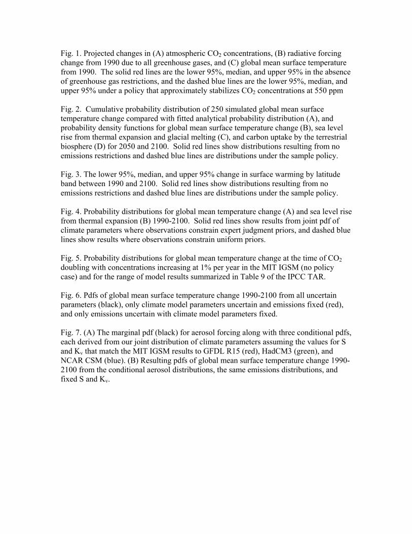
Fig. 1. Projected changes in (A) atmospheric CO2 concentrations, (B) radiative forcing change from 1990 due to all greenhouse gases, and (C) global mean surface temperature from 1990. The solid red lines are the lower 95%, median, and upper 95% in the absence of greenhouse gas restrictions, and the dashed blue lines are the lower 95%, median, and upper 95% under a policy that approximately stabilizes CO2 concentrations at 550 ppm Fig. 2. Cumulative probability distribution of 250 simulated global mean surface temperature change compared with fitted analytical probability distribution (A), and probability density functions for global mean surface temperature change (B), sea level rise from thermal expansion and glacial melting (C), and carbon uptake by the terrestrial biosphere (D) for 2050 and 2100. Solid red lines show distributions resulting from no emissions restrictions and dashed blue lines are distributions under the sample policy. Fig. 3. The lower 95%, median, and upper 95% change in surface warming by latitude band between 1990 and 2100. Solid red lines show distributions resulting from no emissions restrictions and dashed blue lines are distributions under the sample policy. Fig. 4. Probability distributions for global mean temperature change (A) and sea level rise from thermal expansion (B) 1990-2100. Solid red lines show results from joint pdf of climate parameters where observations constrain expert judgment priors, and dashed blue lines show results where observations constrain uniform priors. Fig. 5. Probability distributions for global mean temperature change at the time of CO2 doubling with concentrations increasing at 1% per year in the MIT IGSM (no policy case) and for the range of model results summarized in Table 9 of the IPCC TAR. Fig. 6. Pdfs of global mean surface temperature change 1990-2100 from all uncertain parameters (black), only climate model parameters uncertain and emissions fixed (red), and only emissions uncertain with climate model parameters fixed. Fig. 7. (A) The marginal pdf (black) for aerosol forcing along with three conditional pdfs, each derived from our joint distribution of climate parameters assuming the values for S and Kv that match the MIT IGSM results to GFDL R15 (red), HadCM3 (green), and NCAR CSM (blue). (B) Resulting pdfs of global mean surface temperature change 1990-2100 from the conditional aerosol distributions, the same emissions distributions, and fixed S and Kv.

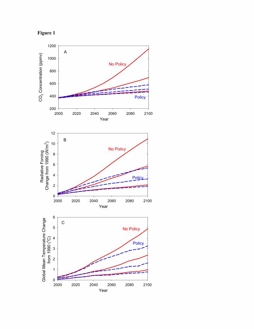
Figure 1

Year2000 2020 2040 2060 2080 2100

Rad

iativ

e Fo

rcin

g C

hang

e fro

m 1

990

(W/m

2 )

0

2

4

6

8

10

12

Policy

B

Year2000 2020 2040 2060 2080 2100

CO

2 Con

cent

ratio

n (p

pmv)

200

400

600

800

1000

1200A

Policy

Year2000 2020 2040 2060 2080 2100

Glo

bal M

ean

Tem

pera

ture

Cha

nge

from

199

0 (o C

)

0

1

2

3

4

5

6

Policy

C

No Policy

No Policy

No Policy

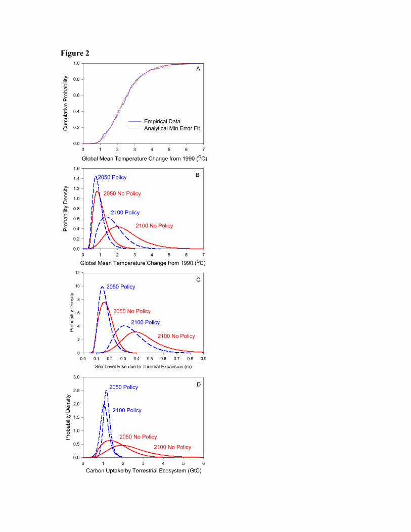
Figure 2

A

Global Mean Temperature Change from 1990 (oC)0 1 2 3 4 5 6 7

Cum

ulat

ive

Prob

abilit

y

0.0

0.2

0.4

0.6

0.8

1.0

Empirical DataAnalytical Min Error Fit

Global Mean Temperature Change from 1990 (oC)0 1 2 3 4 5 6 7

Prob

abilit

y D

ensi

ty

0.0

0.2

0.4

0.6

0.8

1.0

1.2

1.4

1.6B

2100 Policy

2050 Policy

Carbon Uptake by Terrestrial Ecosystem (GtC)0 1 2 3 4 5 6

Prob

abilit

y D

ensi

ty

0.0

0.5

1.0

1.5

2.0

2.5

3.0

D

2100 Policy

2050 Policy

Sea Level Rise due to Thermal Expansion (m)

0.0 0.1 0.2 0.3 0.4 0.5 0.6 0.7 0.8 0.9

Prob

abilit

y D

ensi

ty

0

2

4

6

8

10

12

C

2100 Policy

2050 Policy

2100 No Policy

2050 No Policy

2100 No Policy

2050 No Policy

2100 No Policy

2050 No Policy

Figure 3

Latitude

-80 -60 -40 -20 0 20 40 60 80

Zona

l Mea

n Te

mpe

ratu

re C

hang

e19

90-2

100

(oC

)

0

2

4

6

8

10

12

14

Policy

No Policy

Figure 4

Global Mean Temperature Change from 1990 (oC)

0 1 2 3 4 5 6 7 8

Prob

abilit

y D

ensi

ty

0.0

0.1

0.2

0.3

0.4

0.5

Sea Level Rise due to Thermal Expansion (m)

0.0 0.1 0.2 0.3 0.4 0.5 0.6 0.7 0.8 0.9 1.0 1.1 1.2

Prob

abilit

y D

ensi

ty

0.0

0.5

1.0

1.5

2.0

2.5

3.0

3.5

A

B

Posterior from Uniform Priors

Posterior from Uniform Priors

Posterior from Expert Priors

Posterior from Expert Priors

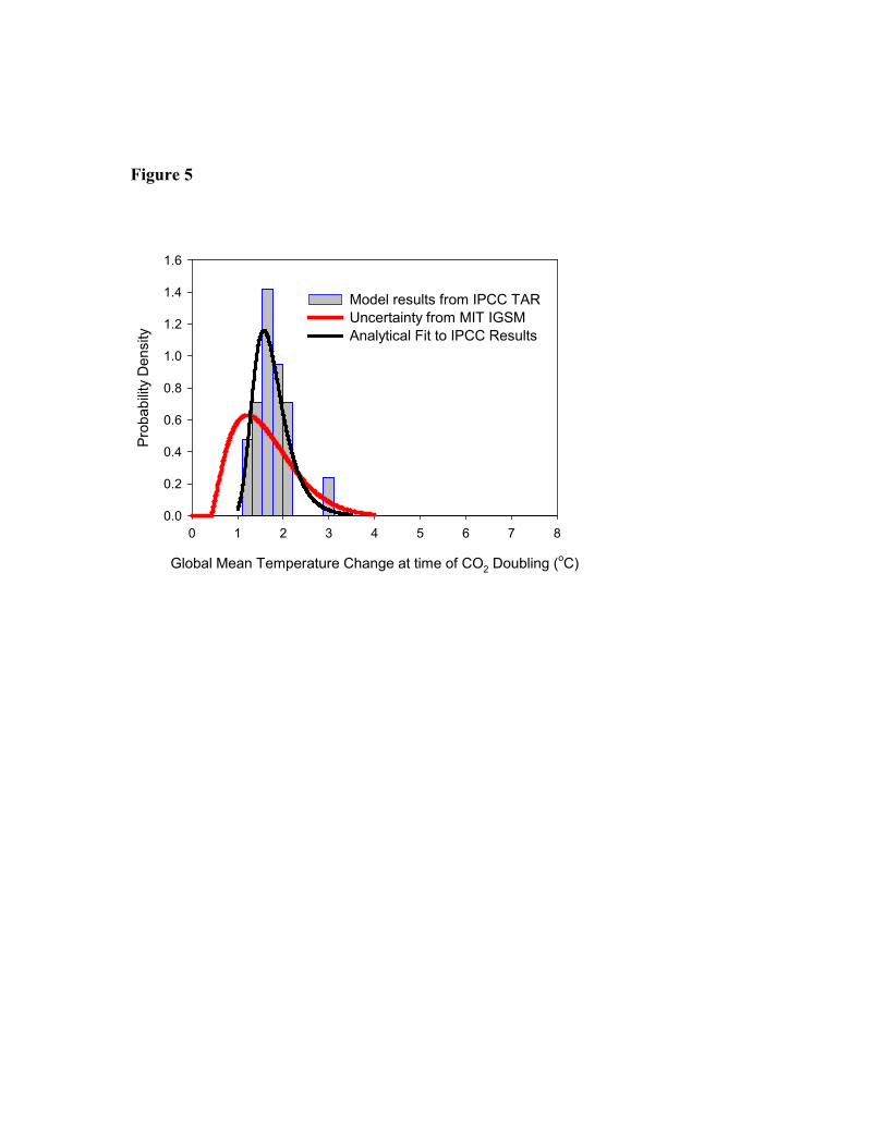
Figure 5

Global Mean Temperature Change at time of CO2 Doubling (oC)

0 1 2 3 4 5 6 7 8

Prob

abilit

y D

ensi

ty

0.0

0.2

0.4

0.6

0.8

1.0

1.2

1.4

1.6

Model results from IPCC TARUncertainty from MIT IGSMAnalytical Fit to IPCC Results

Figure 6

Global Mean Temperature Change 1990-2100 (oC)0 1 2 3 4 5 6 7

Prob

abilit

y D

ensi

ty

0.0

0.2

0.4

0.6

0.8

1.0MIT IGSM: Full UncertaintyIGSM: Only Climate Parameters UncertainIGSM: Only Emissions Parameters Uncertain

Figure 7

Global Mean Temperature Change 1990-2100 (oC)0 1 2 3 4 5 6 7

Prob

abilit

y D

ensi

ty

0.0

0.2

0.4

0.6

0.8MIT IGSM: Full UncertaintyGFDL_R15HadCM3NCAR CSM

B

Aerosol Forcing Strength (w/m2)0.0 0.1 0.2 0.3 0.4 0.5 0.6 0.7 0.8 0.9 1.0 1.1

Prob

abilit

y D

ensi

ty

0

1

2

3

4

5

6Marginal PDF - uncertainty in S and KvConditional - GFDL_R15Conditional - HADCM3Conditional - NCAR_CSM

A