
Unbiased Recommender Learning from Missing-Not-At-Random ...
9
Unbiased Recommender Learning from Missing-Not-At-Random Implicit Feedback Yuta Saito Tokyo Institute of Technology [email protected] Suguru Yaginuma SMN Corporation [email protected] Yuta Nishino SMN Corporation [email protected] Hayato Sakata SMN Corporation [email protected] Kazuhide Nakata Tokyo Institute of Technology [email protected] ABSTRACT Recommender systems widely use implicit feedback such as click data because of its general availability. Although the presence of clicks signals the users’ preference to some extent, the lack of such clicks does not necessarily indicate a negative response from the users, as it is possible that the users were not exposed to the items (positive-unlabeled problem). This leads to a difficulty in predicting the users’ preferences from implicit feedback. Previous studies addressed the positive-unlabeled problem by uniformly upweighting the loss for the positive feedback data or estimat- ing the confidence of each data having relevance information via the EM-algorithm. However, these methods failed to address the missing-not-at-random problem in which popular or frequently recommended items are more likely to be clicked than other items even if a user does not have a considerable interest in them. To overcome these limitations, we first define an ideal loss function to be optimized to realize recommendations that maximize the relevance and propose an unbiased estimator for the ideal loss. Subsequently, we analyze the variance of the proposed unbiased estimator and further propose a clipped estimator that includes the unbiased estimator as a special case. We demonstrate that the clipped estimator is expected to improve the performance of the recommender system, by considering the bias-variance trade-off. We conduct semi-synthetic and real-world experiments and demon- strate that the proposed method largely outperforms the baselines. In particular, the proposed method works better for rare items that are less frequently observed in the training data. The findings indi- cate that the proposed method can better achieve the objective of recommending items with the highest relevance. CCS CONCEPTS • Information systems → Collaborative filtering; • Comput- ing methodologies → Learning from implicit feedback. Permission to make digital or hard copies of all or part of this work for personal or classroom use is granted without fee provided that copies are not made or distributed for profit or commercial advantage and that copies bear this notice and the full citation on the first page. Copyrights for components of this work owned by others than ACM must be honored. Abstracting with credit is permitted. To copy otherwise, or republish, to post on servers or to redistribute to lists, requires prior specific permission and/or a fee. Request permissions from [email protected]. WSDM ’20, February 3–7, 2020, Houston, TX, USA © 2020 Association for Computing Machinery. ACM ISBN 978-1-4503-6822-3/20/02. . . $15.00 https://doi.org/10.1145/3336191.3371783 KEYWORDS Implicit Feedback; Missing-Not-At-Random; Inverse Propensity Weighting; Positive-Unlabeled Learning; Matrix Factorization. ACM Reference Format: Yuta Saito, Suguru Yaginuma, Yuta Nishino, Hayato Sakata, and Kazuhide Nakata. 2020. Unbiased Recommender Learning from Missing-Not-At-Random Implicit Feedback. In The Thirteenth ACM International Conference on Web Search and Data Mining (WSDM ’20), February 3–7, 2020, Houston, TX, USA. ACM, New York, NY, USA, 9 pages. https://doi.org/10.1145/3336191.3371783 1 INTRODUCTION Recommender systems are widely used in industries such as per- sonalized advertising and video streaming [3, 9, 10]. These services utilize recommender systems to predict and provide users with items that they may be interested in to improve user experience. To provide such recommendations, predicting the items that users like is an important task [7, 9, 16]. Generally, one can use two types of data for the recommendation. One includes users’ ratings on items, and the other corresponds to users’ clicks (e.g., purchases, views) [9, 17]. Rating data is called explicit data, as they represent the preferences explicitly via positive or negative feedback. Typically, collecting sufficient explicit data for recommendation is difficult because it requires users to actively provide ratings [9]. In contrast, click data, which is called implicit data, are easy to collect because they represent the behavior logs of the users [10]. Any services, even those without the users’ ratings, can utilize the data, and many of the actual recommender systems are based on implicit data [9, 19]. As in the information retrieval field [11, 12, 17, 27], one should estimate the relevance of an item to a user from implicit feedback to improve user experience, because one can recommend items that users are genuinely interested in by accurately predicting its relevance. However, as the implicit data is not the explicit feedback of the users’ preferences, one cannot know whether unclicked feedback is negative feedback or unlabeled positive feedback; this corresponds to the positive- unlabeled problem [2, 5, 9]. To predict the relevance, [7] proposed weighted matrix factor- ization (WMF), which assigns unclicked items less weight to incor- porate the idea that those items correspond to less confidence in prediction than clicked items. However, in some cases, one might be more confident in predicting the relevance of some unclicked items than for the other unclicked ones. Unclicked items that have been recommended several times indicate that they are less relevant for the users. Exposure matrix factorization (ExpoMF) fully utilizes this arXiv:1909.03601v3 [stat.ML] 9 Feb 2020
Transcript of Unbiased Recommender Learning from Missing-Not-At-Random ...

Unbiased Recommender Learning fromMissing-Not-At-Random Implicit Feedback
Yuta Saito
Tokyo Institute of Technology
Suguru Yaginuma
SMN Corporation
Yuta Nishino
SMN Corporation
Hayato Sakata
SMN Corporation
Kazuhide Nakata
Tokyo Institute of Technology
ABSTRACTRecommender systems widely use implicit feedback such as click
data because of its general availability. Although the presence of
clicks signals the users’ preference to some extent, the lack of
such clicks does not necessarily indicate a negative response from
the users, as it is possible that the users were not exposed to the
items (positive-unlabeled problem). This leads to a difficulty in
predicting the users’ preferences from implicit feedback. Previous
studies addressed the positive-unlabeled problem by uniformly
upweighting the loss for the positive feedback data or estimat-
ing the confidence of each data having relevance information via
the EM-algorithm. However, these methods failed to address the
missing-not-at-random problem in which popular or frequently
recommended items are more likely to be clicked than other items
even if a user does not have a considerable interest in them. To
overcome these limitations, we first define an ideal loss function
to be optimized to realize recommendations that maximize the
relevance and propose an unbiased estimator for the ideal loss.
Subsequently, we analyze the variance of the proposed unbiased
estimator and further propose a clipped estimator that includes
the unbiased estimator as a special case. We demonstrate that the
clipped estimator is expected to improve the performance of the
recommender system, by considering the bias-variance trade-off.
We conduct semi-synthetic and real-world experiments and demon-
strate that the proposed method largely outperforms the baselines.
In particular, the proposed method works better for rare items that
are less frequently observed in the training data. The findings indi-
cate that the proposed method can better achieve the objective of
recommending items with the highest relevance.
CCS CONCEPTS• Information systems → Collaborative filtering; • Comput-ing methodologies → Learning from implicit feedback.
Permission to make digital or hard copies of all or part of this work for personal or
classroom use is granted without fee provided that copies are not made or distributed
for profit or commercial advantage and that copies bear this notice and the full citation
on the first page. Copyrights for components of this work owned by others than ACM
must be honored. Abstracting with credit is permitted. To copy otherwise, or republish,
to post on servers or to redistribute to lists, requires prior specific permission and/or a
fee. Request permissions from [email protected].
WSDM ’20, February 3–7, 2020, Houston, TX, USA© 2020 Association for Computing Machinery.
ACM ISBN 978-1-4503-6822-3/20/02. . . $15.00
https://doi.org/10.1145/3336191.3371783
KEYWORDSImplicit Feedback; Missing-Not-At-Random; Inverse Propensity
Weighting; Positive-Unlabeled Learning; Matrix Factorization.
ACM Reference Format:Yuta Saito, Suguru Yaginuma, Yuta Nishino, Hayato Sakata, and Kazuhide
Nakata. 2020. Unbiased Recommender Learning fromMissing-Not-At-Random
Implicit Feedback. In The Thirteenth ACM International Conference on WebSearch and Data Mining (WSDM ’20), February 3–7, 2020, Houston, TX, USA.ACM, New York, NY, USA, 9 pages. https://doi.org/10.1145/3336191.3371783
1 INTRODUCTIONRecommender systems are widely used in industries such as per-
sonalized advertising and video streaming [3, 9, 10]. These services
utilize recommender systems to predict and provide users with
items that they may be interested in to improve user experience.
To provide such recommendations, predicting the items that users
like is an important task [7, 9, 16].
Generally, one can use two types of data for the recommendation.
One includes users’ ratings on items, and the other corresponds to
users’ clicks (e.g., purchases, views) [9, 17]. Rating data is called
explicit data, as they represent the preferences explicitly via positive
or negative feedback. Typically, collecting sufficient explicit data
for recommendation is difficult because it requires users to actively
provide ratings [9]. In contrast, click data, which is called implicit
data, are easy to collect because they represent the behavior logs of
the users [10]. Any services, even those without the users’ ratings,
can utilize the data, and many of the actual recommender systems
are based on implicit data [9, 19]. As in the information retrieval
field [11, 12, 17, 27], one should estimate the relevance of an item to
a user from implicit feedback to improve user experience, because
one can recommend items that users are genuinely interested in
by accurately predicting its relevance. However, as the implicit
data is not the explicit feedback of the users’ preferences, one
cannot know whether unclicked feedback is negative feedback
or unlabeled positive feedback; this corresponds to the positive-
unlabeled problem [2, 5, 9].
To predict the relevance, [7] proposed weighted matrix factor-
ization (WMF), which assigns unclicked items less weight to incor-
porate the idea that those items correspond to less confidence in
prediction than clicked items. However, in some cases, one might be
more confident in predicting the relevance of some unclicked items
than for the other unclicked ones. Unclicked items that have been
recommended several times indicate that they are less relevant for
the users. Exposure matrix factorization (ExpoMF) fully utilizes this
arX
iv:1
909.
0360
1v3
[st
at.M
L]
9 F
eb 2
020

exposure information [17]. The authors introduced exposure vari-
ables and the latent probabilistic model, in which the probability of
a click is the product of the probability of the exposure and rele-
vance level. Under this probabilistic model, when a user has been
exposed to an item, clicked and unclicked information between
the pair can be regarded as relevance information. Thus, ExpoMF
upweights the loss of data with high exposure probability because
the exposure probability is regarded as the confidence of how much
relevance information each data includes. Although ExpoMF tack-
les the positive-unlabeled problem by introducing the exposure
variables, it does not address another critical issue of implicit feed-
back recommendation, namely the missing-not-at-random (MNAR)
problem [18, 23, 28]. This is because, by upweighting the loss of
data with high exposure probability (mostly popular items), it can
lead to poor prediction accuracy for rare items. Thus, ExpoMF suf-
fers from bias and cannot achieve the objective of recommender
systems to provide users with items that are relevant to them.
In this study, to establish a method to predict items with the high-
est relevance rather than the highest click probability, we first define
the ideal loss function that should be optimized tomaximize the rele-
vance. We theoretically demonstrate that the existing methods (e.g.,
WMF, ExpoMF) have biases in their loss functions toward the ideal
loss. Next, we simultaneously solve the positive-unlabeled problem
and the MNAR problem inspired by the estimation technique for
causal inference [8, 20, 21] and derive an unbiased estimator for
the ideal loss estimated only from the observable feedback. Fur-
ther, we analyze the variance of the proposed unbiased estimator
and highlight that the variance could be large under recommenda-
tion settings. Moreover, we propose a clipped estimator that could
achieve a better bias-variance trade-off than that of the unbiased es-
timator and investigate its theoretical characteristics. Finally, in the
experiments, we verify the effectiveness of the proposed method
on both semi-synthetic and real-world datasets.
The contributions of this research are as follows.
• We define an ideal loss function to be optimized to maximize
relevance. We propose an unbiased estimator for the loss
function of interest for the first time.
• We perform theoretical analyses for the statistical proper-
ties of the proposed estimator and indicate that its variance
could be large. We address the variance problem by using a
variance reduction estimator.
• We conduct experiments using semi-synthetic and real-world
datasets. Compared to the baselines, the proposed method
largely improves the rankingmetrics. In addition, it improves
the prediction for the less popular items, which comprise a
major proportion of the total items.
2 NOTATION AND PROBLEM FORMULATIONIn this section, we introduce the basic notation and formulate the
implicit feedback recommendation.
2.1 NotationLet u ∈ U be a user (|U|= m), i ∈ I be an item (|I |= n), andD = U × I be the set of all user–item pairs. Y ∈ {0, 1}m×n
is a
click matrix, and each entry Yu,i is a Bernoulli random variable
representing a click between the user u and item i . If the feedback
of (u, i) is observed, then Yu,i = 1; otherwise, Yu,i = 0. In implicit
feedback recommendation, Yu,i = 1 indicates a positive feedback,
but Yu,i = 0 is either a negative or unlabeled positive feedback. To
precisely formulate this implicit feedback setting, we introduce two
other matrices. R ∈ {0, 1}m×nis a relevance matrix, and each entry
Ru,i is a Bernoulli random variable representing the relevance
of user u and item i . Ru,i = 1 means that u and i are relevant;
however, Ru,i = 0 means that u and i are irrelevant. The other
matrix is called the exposure matrix, denoted as O ∈ {0, 1}m×n.
Each entry of this matrix Ou,i is a random variable representing
whether user u has been exposed to item i . It should be noted
that in implicit feedback recommendation, both the relevance and
exposure random variables are unobserved, and only click randomvariables are observable.
In this work, we make the following two assumptions for all
user–item pairs.
Yu,i = Ou,i · Ru,i (1)
P (Yu,i = 1) = θu,i · γu,i (2)
We define θu,i = P(Ou,i = 1
)and γu,i = P
(Ru,i = 1
)as the expo-
sure and relevance parameters, respectively and assume that both
parameters are non-zero for all user–item pairs.
Eq. (1) assumes that item i is clicked by user u if i has beenexposed to u and they are relevant (i.e., Yu,i = 1 ⇔ Ou,i = 1 =
1 & Ru,i = 1 ). The position-based model in unbiased learning-to-
rank [12, 27] makes the same assumption in the click generative
process. This assumption precisely represents the implicit feedback
setting, in which a click does not always signify relevance.
In contrast, Eq. (2) assumes that the click probability is decom-
posed into the exposure probability (θu,i ) and relevance level
(γu,i )1. Given this assumption, the exposure probability θu,i can
take different values among user–item pairs, and it can model the
MNAR setting in which the click probability and relevance level
are not proportional.
2.2 True Performance MetricThis section describes the objective of this study. To evaluate the
recommendation policy with implicit feedback data, the top-N rec-
ommendation metrics such as the mean average precision (MAP)
and recall are commonly used [28]. In general, these metrics can
be defined in the following manner [28].
Rclick
(Z)
=
1
|U|∑u ∈U
∑i ∈I
P(Yu,i = 1
)︸ ︷︷ ︸click probability
·c(Zu,i
)(3)
where Z = {Zu,i }(u,i )∈D is the predicted ranking of item i for useru, and the function c(·) characterizes a top-N scoring metric. For
example, for DCG@K, the function is defined as c(Zu,i ) = I{Zu,i ≤K}/log(Zu,i + 1).
The problem is that click (Yu,i ) does not directly signify relevance(Ru,i ), and thus, the top-N recommendation metrics defined as in
Eq. (3) are not appropriate to measure the improvement in the user
experience. Therefore, we use the following top-N recommendation
1This assumption is similar to the unconfoundedness assumption in causal inference
[8, 20, 21] and can also be represented as O ⊥ R |u, i .

metric defined using the relevance level as the performance metric.
Rr el
(Z)
=
1
|U|∑u ∈U
∑i ∈I
P(Ru,i = 1
)︸ ︷︷ ︸relevance level
·c(Zu,i
)(4)
The focus of this study is to optimize the performance metric in
Eq. (4). To achieve this goal, we follow the basic pointwise approach
and aim to optimize the following loss function of interest.
Lideal
(R)
=
1
|D|∑
(u,i )∈D
[γu,iδ
(1)
(Ru,i
)+
(1 − γu,i
)δ (0)
(Ru,i
)](5)
where R is a prediction matrix, and δ (R), (R ∈ {0, 1}) denotes thelocal loss for user–item pair (u, i). For example, when δ (R)
(R) =
−(R log(R) + (1−R) log(1− R)), then Lideal (R) is called the log loss.
In the following sections, we denote δ (R)(Ru,i ) simply as δ
(R)
u,i .
A prediction matrix R minimizing the ideal loss defined using
the relevance level in Eq. (5) is expected to lead to the desired values
of the top-N recommendation metric in Eq. (4).
3 ANALYSIS ON EXISTING BASELINESIn this section, we describe the standard baselines and theoretically
analyze the loss functions used in these methods. In particular, we
demonstrate that the loss functions are biased against the ideal loss.
3.1 Weighted Matrix FactorizationWMF is the most basic latent factor model for implicit feedback
recommendation [7]. The WMF uses a simple heuristic in which
all the clicked data are equally upweighted compared with the
unclicked data [7, 17]. This model optimizes the following estimator
for the ideal loss:
LWMF
(R)
=
1
|D|∑
(u,i )∈D
[cYu,iδ
(1)
u,i +
(1 − Yu,i
)δ
(0)
u,i
](6)
where c ≥ 1 is a hyperparameter representing the confidence of
the clicked data relative to that of the unclicked data. When no side
information is available, c is uniform among all the clicked data. In
the following proposition, we demonstrate that the estimator used
in the WMF is biased.
Proposition 3.1. (Bias of WMF estimator) The bias of the estima-tor used in WMF is represented as follows.���E [
LWMF
(R)]
− Lideal
(R)���
=
1
|D|
����� ∑(u,i )∈D
[(cθu,i − 1)γu,iδ
(1)+ γu,i (1 − θu,i )δ
(0)
u,i
] �����Proof.
E[LWMF
(R)]
= E
[1
|D|∑
(u,i )∈D
[cYu,iδ
(1)
u,i +
(1 − Yu,i
)δ
(0)
u,i
] ]=
1
|D|∑
(u,i )∈D
[cE
[Yu,i
]δ
(1)
u,i +
(1 − E
[Yu,i
] )δ
(0)
u,i
]=
1
|D|∑
(u,i )∈D
[cθu,iγu,iδ
(1)
u,i +
(1 − θu,iγu,i
)δ
(0)
u,i
]
Thus,
E[LWMF
(R)]
− Lideal
(R)
=
1
|D|∑
(u,i )∈D
[cθu,iγu,iδ
(1)
u,i +
(1 − θu,iγu,i
)δ
(0)
u,i
]− 1
|D|∑
(u,i )∈D
[γu,iδ
(1)
u,i +
(1 − γu,i
)δ
(0)
u,i
]=
1
|D|∑
(u,i )∈D
[(cθu,i − 1)γu,iδ
(1)+ γu,i (1 − θu,i )δ
(0)
u,i
]□
For LWMF
(R)to be theoretically unbiased, cθu,i − 1 = 0 ⇒
θu,i = 1/c , and 1 − θu,i = 0 ⇒ θu,i = 1 need to be satisfied for
all pairs from the last equation. However, θu,i can take different
values among user–item pairs in our setting; thus, these conditions
are not always satisfied, and the loss function of WMF does not
satisfy the unbiasedness. This is because WMF does not address
the positive-unlabeled problem, in which Y = 0 does not always
signify R = 0. Thus, WMF is unsuitable for optimizing our metric
of interest defined in Eq. (4).
3.2 Exposure Matrix FactorizationIn contrast to the WMF, the ExpoMF is a prediction method con-
sidering the exposure matrix (O), and it is based on the following
latent probabilistic model [17]:
U ∼ N(0, λ−1
U IK
), V ∼ N
(0, λ−1
V IK
)Ou,i ∼ Bern (µi ) , Yu,i |Ou,i = 1 ∼ N
(U⊤u Vi , λ
−1
y
)where λU , λV , and λy are the hyperparameters denoting the inverse
variance of the prior distributions, and Bern(·) is the Bernoulli dis-tribution. Following the probabilistic model defined above, P (Yu,i =
0 |Ou,i = 0) = 1, which is consistent with our assumptions.
The log-likelihood to derive the parameters (i.e., µi ,Uu , and Vi )can be written as
2
log
(P
(ou,i ,yu,i | µu,i ,Uu ,Vi , λ−1
y
))= logBern
(ou,i | µu,i
)+ ou,i · logN
(yu,i |U⊤
u Vi , λ−1
y
)︸ ︷︷ ︸
(a)
(7)
In Eq. (7), the loss to derive the user and item matrices (U ,V ) is (a),
and it can be defined in the following manner:
(a) =
δ (1)
(U⊤u Vi
)(yu,i = 1, ou,i = 1)
δ (0)(U⊤u Vi
)(yu,i = 0, ou,i = 1)
0 otherwise (ou,i = 0)
Therefore, the loss function of the ExpoMF is designed to consider
the local loss of user–item pairs when the item has been exposed
to the user (i.e., ou,i = 1). This is because if an item has been
exposed, the click variable is considered to represent the relevance
information (i.e., Ou,i = 1 ⇒ Yu,i = Ru,i ).
2Equation (2) of [17]. The third term is always 0 and is thus omitted here.

However, the realizations of exposure variables {ou,i } are unob-served. Therefore, ExpoMF uses an EM-like iterative algorithm to
derive the user–item matrices. In the E-step, the posterior exposure
probability is estimated, and in the M-step, the model parameters
are updated to optimize the log-likelihood3. Given the true poste-
rior exposure probabilities, the M-step of ExpoMF is interpreted to
minimize the following weighted loss function.
LExpoMF
(R)
=
1
|D|∑
(u,i )∈Dθ ′u,i
[Yu,iδ
(1)
u,i +
(1 − Yu,i
)δ
(0)
u,i
](8)
where θ ′u,i = E[Ou,i |Yu,i
]is the posterior exposure probability.
For example, E[Ou,i |Yu,i = 1
]= 1 because Yu,i = 1 ⇒ Ou,i = 1.
This posterior probability represents the confidence of the amount
of relevance information contained in click indicator Yu,i .ExpoMF utilizes the posterior probability of the exposure to
reweight data and improves the WMF. However, the following
proposition suggests that the loss function in Eq. (8) optimized in
the M-step of the ExpoMF is also biased against the ideal loss.
Proposition 3.2. (Bias of ExpoMF) When the posterior exposureprobabilities are given, then, the bias of the estimator used in ExpoMFis represented as follows.���E [
LExpoMF
(R)]
− Lideal
(R)���
=
1
|D|
��� ∑(u,i )∈D
γu,i (θ′u,iθu,i − 1)δ
(1)
u,i
+
{θ ′u,i − 1 − γu,i (θu,iθ
′u,i − 1)
}δ
(0)
u,i
���Proof.
E[LExpoMF
(R)]
= E
[1
|D|∑
(u,i )∈Dθ ′u,i
[Yu,iδ
(1)
u,i +
(1 − Yu,i
)δ
(0)
u,i
] ]=
1
|D|∑
(u,i )∈Dθ ′u,i
[E
[Yu,i
]δ
(1)
u,i +
(1 − E
[Yu,i
] )δ
(0)
u,i
]=
1
|D|∑
(u,i )∈D
[θ ′u,iθu,iγu,iδ
(1)
u,i + θ ′u,i(1 − θu,iγu,i
)δ
(0)
u,i
]Thus we obtain:
E[LExpoMF
(R)]
− Lideal
(R)
=
1
|D|∑
(u,i )∈D
[θ ′u,iθu,iγu,iδ
(1)
u,i + θ ′u,i(1 − θu,iγu,i
)δ
(0)
u,i
]− 1
|D|∑
(u,i )∈D
[γu,iδ
(1)
u,i +
(1 − γu,i
)δ
(0)
u,i
]=
1
|D|∑
(u,i )∈D
[γu,i (θ
′u,iθu,i−1)δ
(1)
u,i +
{θ ′u,i−1−γu,i (θu,iθ ′u,i−1)
}δ
(0)
u,i
]□
For LExpoMF
(R)to be theoretically unbiased, θu,iθ
′u,i − 1 =
0 ⇒ θu,iθ′u,i = 1, and θ ′u,i − 1 = 0 ⇒ θ ′u,i = 1 need to be satisfied
for all pairs from the last equation. However, θu,i and θ′u, j can take
different values among user–item pairs in our setting, and thus,
3The detailed learning procedure of ExpoMF is described in Section 3.3 of [17].
these conditions are not always satisfied, and the loss function of
the ExpoMF does not satisfy the unbiasedness. This is because the
ExpoMF upweights the local loss of data that is frequently observed
in the training data (i.e., data having high exposure probability).
This upweighting leads to the poor prediction accuracy for data
having low exposure probability such as tail items, and thus, it fails
to achieve the goal of recommender systems. Therefore, dealing
with the MNAR problem as well as the unlabeled nature of implicit
feedback is essential to derive a desirable estimator.
4 PROPOSED METHODIn this section, we propose an unbiased estimator for the ideal loss
to overcome the limitations described in the previous section. The
proposed unbiased estimator is an extension of the Inverse Propen-
sity Score (IPS) in causal inference [8, 20, 21] and an estimator in
positive-unlabeled learning [2, 15]. In our theoretical analysis, we
prove that our estimator is valid in the implicit recommendation
setting. Moreover, we analyze the variance of the unbiased estima-
tor and indicate that it can suffer from a high variance. Finally, we
provide and analyze a technique to address the variance problem.
4.1 Proposed EstimatorFirst, we define the propensity score to deal with theMNARproblem
of implicit feedback as follows.
Definition 4.1. (Propensity Score) The propensity score of user–
item pair (u, i) is
θu,i = P (Ou,i = 1) = P(Yu,i = 1 | Ru,i = 1
)Next, our proposed estimator is defined using the propensity
score.
Definition 4.2. (Unbiased Estimator) When the propensity scores
are given, the unbiased estimator is defined as
Lunbiased
(R)
=
1
|D|∑
(u,i )∈D
[Yu,iθu,i
δ(1)
u,i +
(1 −
Yu,iθu,i
)δ
(0)
u,i
](9)
Note that this unbiased estimator is not the standard form of
the IPS estimator in the explicit feedback setting [23] because one
cannot use the exposure indicator in the implicit feedback setting.
The proposed estimator can also be represented in the following
form.
1
|D|∑
(u,i )∈D
[Yu,i
(1
θu,iδ
(1)
u,i +
(1 − 1
θu,iδ
(0)
u,i
))+ (1 − Yu,i )δ
(0)
u,i
]Thus, the unbiased estimator applies both positive loss (δ (1)
) and
negative loss (δ (0)) for the clicked data (Yu,i = 1). In the follow-
ing proposition, we show that our unbiased estimator is unbiased
against the ideal loss.
Proposition 4.3. The unbiased estimator defined in Eq. (9) isunbiased against the ideal loss in Eq. (5).
E[Lunbiased
(R)]
= Lideal
(R)

Proof.
E[Lunbiased
(R)]
= E
[1
|D|∑
(u,i )∈D
[Yu,iθu,i
δ(1)
u,i +
(1 −
Yu,iθu,i
)δ
(0)
u,i
] ]=
1
|D|∑
(u,i )∈D
[E[Yu,i ]
θu,iδ
(1)
u,i +
(1 −E[Yu,i ]
θu,i
)δ
(0)
u,i
]=
1
|D|∑
(u,i )∈D
[γu,iδ
(1)
u,i +
(1 − γu,i
)δ
(0)
u,i
]= Lideal
(R)□
Proposition 4.3 validates that de-biasing using propensity reweight-
ing is valid inMNAR implicit recommendation. However, propensity-
based estimators often suffer from a high variance [4, 22, 25]. More-
over, variance analysis was not conducted in a previous study on
positive-unlabeled learning [2, 15]. Thus, in the following theorem,
we provide the variance of the unbiased estimator.
Theorem 4.4. (Variance of the unbiased estimator) Given sets ofindependent random variables {Yu,i }, {Ou,i }, and {Ru,i }, propensityscores {θu,i }, and predicted matrix R, the variance of the unbiasedestimator is
V(Lunbiased
(R))
=
1
|D|2∑
(u,i )∈Dγu,i
(1
θu,i− γu,i
) (δ
(1)
u,i − δ(0)
u,i
)2
Proof. First, we define Xu,i =Yu,iθu,i
δ(1)
u,i +
(1 − Yu,i
θu,i
)δ
(0)
u,i . Subse-
quently, V(Xu,i
)can be written as
V(Xu,i
)= E
[(Xu,i )
2]︸ ︷︷ ︸
(b)
−(E
[Xu,i
] )2︸ ︷︷ ︸
(c )
By Proposition 4.3,
(c) = (γu,iδ(1)
u,i + (1 − γu,i )δ(0)
u,i )2
= γ 2
u,i (δ(1)
u,i )2
+ 2γu,i (1 − γu,i )δ(1)
u,iδ(0)
u,i + (1 − γu,i )2(δ
(0)
u,i )2
Then,
X 2
u,i =
Yu,i
θ2
u,i(δ
(1)
u,i )2
+ 2
Yu,iθu,i
(1−
Yu,iθu,i
)δ
(1)
u,iδ(0)
u,i +
(1−
Yu,iθu,i
)2
(δ(1)
u,i )2
=
Yu,i
θ2
u,i(δ
(1)
u,i )2
+ 2
(Yu,iθu,i
−Yu,i
θ2
u,i
)δ
(1)
u,iδ(0)
u,i
+
(1 − 2
Yu,iθu,i
+
Yu,i
θ2
u,i
)(δ
(0)
u,i )2
where Y 2
u,i = Yu,i and (1−Yu,i )2
= (1−Yu,i ). Next, (b) is calculated
as
(b) =
γu,iθu,i
(δ(1)
u,i )2
+ 2
(γ − γ
θu,i
)δ
(1)
u,iδ(0)
u,i +
(1 − 2γ +
γ
θu,i
)(δ
(0)
u,i )2
Therefore,
V(Xu,i
)= (b) − (c) = γu,i
(1
θu,i− γu,i
) (δ
(1)
u,i − δ(0)
u,i
)2
From the assumptions, {Xu,i } is a set of independent random vari-
ables. Thus,
V(Lunbiased
(R))
=
1
|D|2∑
(u,i )∈DV
(Xu,i
)=
1
|D|2∑
(u,i )∈Dγu,i
(1
θu,i− γu,i
) (δ
(1)
u,i − δ(0)
u,i
)2
□
As shown in Theorem 4.4, the variance of the unbiased estimator
depends on the inverse of the propensity score. The propensity
score is defined as the exposure probability, and thus it can be
small, especially for tail items [28]. Therefore, the variance of the
proposed estimator can be large in the implicit recommendation
setting.
4.2 Variance Reduction TechniqueIn the theoretical analysis, we demonstrated that the proposed
unbiased estimator is unbiased against the ideal loss. However,
Theorem 4.4 suggests that the unbiased estimator can suffer from
high variance. In this subsection, we apply the propensity clipping
technique [4, 6, 24] to our estimator and analyze the bias-variance
trade-off of an estimator with clipping.
First, we introduce the propensity score with the clipping tech-
nique.
Definition 4.5. (Clipped Propensity Score) M is a positive con-
stant that takes values in the interval [0, 1]. Then, the clipped
propensity score is defined as:
¯θu,i = max{θu,i ,M} (10)
The clipped propensity score clips a small value of θ byM . We
further define the clipped estimator for the ideal loss by using the
clipped propensity score.
Definition 4.6. (Clipped Estimator) The clipped estimator for the
ideal loss is defined as
Lclipped
(R)
=
1
|D|∑
(u,i )∈D
[Yu,i¯θu,i
δ(1)
u,i +
(1 −
Yu,i¯θu,i
)δ
(0)
u,i
](11)
AsM → 1, the clipped estimator approaches the naive estimator
(estimator of WMF with c = 1); in contrast, asM → 0, it approaches
the unbiased estimator. Thus, the clipped estimator is a general
form of the two estimators. By definition, the inverse of the clipped
propensity score is always smaller than that of the propensity score.
Thus, using the clipped estimator reduces the effect of the variance
problem of the unbiased estimator. However, it introduces some
bias because the clipped propensity score is not always equal to the
true propensity. We provide the bias and variance of the clipped
estimator as follows.
Proposition 4.7. (Bias of the clipped estimator) Given a constantM ∈ [0, 1], the bias of the clipped estimator is���E [
Lclipped
(R)]
− Lideal
(R)���
=
����� 1
|D|∑
(u,i )∈DI{θu,i ≤ M}γu,i
(θu,iM
− 1
) (δ
(1)
u,i − δ(0)
u,i
)�����

Proof. First, we define Xu,i =Yu,iθu,i
δ(1)
u,i +
(1 − Yu,i
θu,i
)δ
(0)
u,i , then,
E[Lclipped
(R)]
=
1
|D|∑
(u,i )∈DI{θu,i > M}E[Xu,i ]
+
1
|D|∑
(u,i )∈DI{θu,i ≤ M} E
[Yu,iM
δ(1)
u,i +
(1 −
Yu,iM
)δ
(0)
u,i
]︸ ︷︷ ︸
(d )
By using E[Yu,i ] = θu,iγu,i , (d) is calculated as
(d) =
θu,iγu,iM
δ(1)
u,i +
(1 −
θu,iγu,iM
)δ
(0)
u,i
By Proposition 4.3, E[Xu,i
]= γu,iδ
(1)
u,i + (1 − γu,i )δ(0)
u,i . Then, the
ideal loss can also be represented as
Lideal
(R)
=
1
|D|∑
(u,i )∈DI{θu,i > M}E[Xu,i ] + I{θu,i ≤ M}E[Xu,i ]
Therefore,
E[Lclipped
(R)]
− Lideal
(R)
=
1
|D|∑
(u,i )∈DI{θu,i ≤ M}
((d) − E[Xu,i ]
)=
1
|D|∑
(u,i )∈D
[I{θu,i ≤ M}γu,i
(θu,iM
− 1
) (δ
(1)
u,i − δ(0)
u,i
)]□
Corollary 4.8. (Variance of the clipped estimator) Under the samecondition as in Theorem 4.4, the variance of the clipped estimator is
V(Lclipped
(R))
=
1
|D|2∑
(u,i )∈Dγu,i
(1
¯θu,i− γu,i
) (δ
(1)
u,i − δ(0)
u,i
)2
≤ V(Lunbiased
(R))∵
1
¯θu,i≤ 1
θu,i
Proof. Propensity scores are not random variables. Thus, we
obtain the variance by replacing θu,i in Theorem 4.4 by¯θu,i . □
As shown above, the clipped estimator always reduces the vari-
ance of the unbiased estimator but introduces some bias depending
on the value ofM . In the experimental part, we tuned the clipping
constantM as a hyper-parameter using a validation set to address
the variance problem.
5 SEMI-SYNTHETIC EXPERIMENTIn this section, we conduct an experiment with semi-synthetic
datasets4and investigate the following research questions (RQs).
RQ1. How does the level of exposure bias affect the performance
of the MF-Naive and MF-Unbiased models?
RQ2. Does optimizing the ideal pointwise loss in Eq. (5) yield a
better value of the ranking metric in Eq. (4)?
4The code is available at https://github.com/usaito/unbiased-implicit-rec.
5.1 Experimental Setup5.1.1 Dataset. We used the MovieLens (ML) 100K dataset
5. This
dataset contains five-star movie ratings collected from a movie
recommendation service, and the ratings are MNAR. To facilitate
ground-truth evaluation against a fully known relevance and expo-
sure parameters, we created these parameters as follows.
1. Using rating-based matrix factorization [14], we found an
approximation of the true ratings as
Ru,i ≈ Ru,i , ∀(u, i) ∈ D
where Ru,i ∈ [1, 5].
2. Using logistic matrix factorization [13], we found an approx-
imation of the true observations as
Ou,i ≈ Ou,i , ∀(u, i) ∈ Dwhere Ou,i is a binary variable representing whether the
rating of (u, i) is observed. If the rating of (u, i) is observed,
Ou,i = 1; otherwise, Ou,i = 0. Thus, Ou,i ∈ (0, 1) is the
estimated probability of observing the rating of (u, i).3. We generate the ground-truth relevance and exposure pa-
rameters as follows.
γu,i = σ (Ru,i − ϵ), θu,i = (Ou,i )p , ∀(u, i) ∈ D
where σ (·) is the sigmoid function, ϵ controls the overall rel-
evance level, and p controls the skewness of the distribution
of the exposure parameter. When a large value of p is used,
then a huge exposure bias is introduced. In the experiment,
we set ϵ = 5 and p = 0.5, 1, 2, 3, 4.
4. Following the probabilistic model described in Eq. (1) and
Eq. (2), we generated click variables as follows.
Ou,i ∼ Bern(θu,i ), Ru,i ∼ Bern(γu,i )
Yu,i = Ou,i · Ru,i , ∀(u, i) ∈ Dwhere Bern(·) is the Bernoulli distribution.
Note that one can evaluate the ground-truth performance of the
methods with the true relevance and exposure parameters by using
semi-synthetic datasets.
5.1.2 Baselines. We used and compared the following models.
• MF-Oracle: The matrix factorization model trained using the
ground truth relevance information. Thus, the performance
of this method is the best achievable performance.
• MF-Naive: The matrix factorization model trained using only
the observable click information. As shown in Proposition
3.1, this estimator has a bias, and this bias problem can be
severe, particularly when a large value of p is used.
• MF-Unbiased: The matrix factorization model trained with
the unbiased loss function defined in Eq. (9). The variance
of the unbiased loss function might be large when a large
value of p is used.
5.1.3 Evaluation Metrics. We used the log-loss and discounted cu-
mulative gain (DCG) on test sets to evaluate the relevance prediction
and the raking performance, respectively. Note that both evaluation
metrics are calculated using the true relevance information, which
is inaccessible when using a real-world dataset.
5http://grouplens.org/datasets/movielens/

Figure 1: (Left) Log-loss on test sets of the MF-Naive and MF-Unbiased models relative to that of the MF-Oracle with differentvalues of p (x-axis). (Others) DCG@K on test sets of the MF-Oracle, MF-Naive, and MF-Unbiased models with different levelsof exposure bias.
5.2 Results & Discussions5.2.1 RQ1. How does the level of exposure bias affect the perfor-mance of the MF-Naive and MF-Unbiased models? Here, we investi-
gate the performance of the MF-Naive and MF-Unbiased models
with different levels of exposure bias (different values of p). Figure1 (left) shows the log-loss on test sets of the MF-Naive and MF-
Unbiased models relative to that of the MF-Oracle model. We report
the results for varying values of p (x-axis).
The figure reveals that the performance of both the MF-Naive
and MF-Unbiased models declines with larger values of p. Thepoor performance of the MF-Naive model with severe exposure
bias is due to the bias problem (stated in Proposition 3.1). On the
other hand, the poor performance of the MF-Unbiased model arises
from the variance problem of the propensity weighting technique
(stated in Theorem 4.4). Although the benefit of using the unbiased
estimator is relatively small when a severe exposure bias exists, it
consistently outperforms the naive estimator in all settings. The
results demonstrate the effectiveness of the unbiased estimation
approach to the different levels of exposure bias.
5.2.2 RQ2. Does the optimization of the ideal pointwise loss actuallylead to a better value of the ranking metric? Next, we compared
the ranking performance of the MF with that of the different es-
timators. Figure 1 shows the DCG@K with different values of K(K ∈ {1, 2, . . . , 10}). We report the results with p = 0.5, 2.0, 4. As
shown in the figure, MF-Unbiased outperforms MF-Naive in all
settings. In particular, with p = 0.5, the MF-Unbiased model largely
outperforms the MF-Naive model and its performance is close to
that of the MF-Oracle model. However, when a large exposure
bias exists (p = 4), the benefit of using the unbiased estimator is
relatively small. These results are well correlated with those for
the relevance level prediction task, as discussed in Section 5.2.1.
Therefore, the results validate that optimizing the ideal pointwise
loss is a valid approach to improving recommendation performance
with respect to the ranking metrics.
6 REAL-WORLD EXPERIMENTIn this section, we compare the prediction methods based on the
proposed estimator and the existing baselines by using a standard
real-world dataset6. In particular, we investigate the following re-
search question.
RQ3. How does the proposed unbiased estimator perform com-
pared with other existing methods?
6.1 Experimental Setup6.1.1 Dataset. We used the Yahoo! R3 dataset
7. This is an explicit
feedback dataset collected from a song recommendation service. As
described in [28], it contains users’ ratings for randomly selected
sets of music as a test set, and thus it can be used to measure the
recommenders’ true performances. The dataset includes explicit
feedback data; we treated items rated greater than or equal to 4
as relevant, and the others were considered irrelevant. We used
this dataset because it contains the training and test sets with
different item and user distributions. Moreover, it contains the
explicit feedback data, thus allowing the utilization of the ground
truth relevance information in the test set. Therefore, this dataset
is appropriate for the evaluation of recommender in the situation
where both positive-unlabeled and MNAR problems exist. To the
best of our knowledge, this dataset is the only one that satisfies
these properties.
6.1.2 Baselines and the proposed model. We describe the existing
baselines and the proposed model used in the real-world experi-
ment.
• Weighted Matrix Factorization (WMF) [7]: The WMF is a
basic baseline model for implicit recommendation and is
described in Section 3.1.
• Exposure Matrix Factorization (ExpoMF) [17]: ExpoMF is
based on the latent probabilistic model using exposure vari-
ables, and it is described in Section 3.2. We used the imple-
mentation provided at https://github.com/dawenl/expo-mf.
• Relevance Matrix Factorization (Rel-MF): Rel-MF is the pro-
posed model and is based on the same latent factor model
as the MF. It updates its user–item factors by minimizing
the clipped version of the proposed estimator in Eq. (11).
We estimated the propensity score by using the following
6The code is available at https://github.com/usaito/unbiased-implicit-rec-real.
7http://webscope.sandbox.yahoo.com/
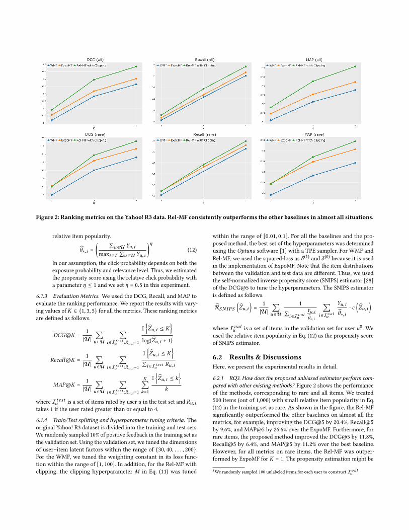
Figure 2: Rankingmetrics on the Yahoo! R3 data. Rel-MF consistently outperforms the other baselines in almost all situations.
relative item popularity.
θ∗,i =
( ∑u ∈U Yu,i
maxi ∈I∑u ∈U Yu,i
)η(12)
In our assumption, the click probability depends on both the
exposure probability and relevance level. Thus, we estimated
the propensity score using the relative click probability with
a parameter η ≤ 1 and we set η = 0.5 in this experiment.
6.1.3 Evaluation Metrics. We used the DCG, Recall, and MAP to
evaluate the ranking performance. We report the results with vary-
ing values of K ∈ {1, 3, 5} for all the metrics. These ranking metrics
are defined as follows.
DCG@K =
1
|U|∑u ∈U
∑i ∈Itestu :Ru,i=1
I{Zu,i ≤ K
}log(Zu,i + 1)
Recall@K =
1
|U|∑u ∈U
∑i ∈Itestu :Ru,i=1
I{Zu,i ≤ K
}∑i ∈Itestu
Ru,i
MAP@K =
1
|U|∑u ∈U
∑i ∈Itestu :Ru,i=1
K∑k=1
I{Zu,i ≤ k
}k
where Itestu is a set of items rated by user u in the test set and Ru,i
takes 1 if the user rated greater than or equal to 4.
6.1.4 Train/Test splitting and hyperparameter tuning criteria. Theoriginal Yahoo! R3 dataset is divided into the training and test sets.
We randomly sampled 10% of positive feedback in the training set as
the validation set. Using the validation set, we tuned the dimensions
of user–item latent factors within the range of {30, 40, . . . , 200}.For the WMF, we tuned the weighting constant in its loss func-
tion within the range of [1, 100]. In addition, for the Rel-MF with
clipping, the clipping hyperparameter M in Eq. (11) was tuned
within the range of [0.01, 0.1]. For all the baselines and the pro-
posed method, the best set of the hyperparameters was determined
using the Optuna software [1] with a TPE sampler. For WMF and
Rel-MF, we used the squared-loss as δ (1)and δ (0)
because it is used
in the implementation of ExpoMF. Note that the item distributions
between the validation and test data are different. Thus, we used
the self-normalized inverse propensity score (SNIPS) estimator [28]
of the DCG@5 to tune the hyperparameters. The SNIPS estimator
is defined as follows.
RSN IPS
(Zu,i
)=
1
|U|∑u ∈U
1∑i ∈Ivalu
Yu,iθ∗,i
∑i ∈Ivalu
Yu,i
θ∗,i· c
(Zu,i
)where Ivalu is a set of items in the validation set for user u8. We
used the relative item popularity in Eq. (12) as the propensity score
of SNIPS estimator.
6.2 Results & DiscussionsHere, we present the experimental results in detail.
6.2.1 RQ3. How does the proposed unbiased estimator perform com-pared with other existing methods? Figure 2 shows the performance
of the methods, corresponding to rare and all items. We treated
500 items (out of 1,000) with small relative item popularity in Eq.
(12) in the training set as rare. As shown in the figure, the Rel-MF
significantly outperformed the other baselines on almost all the
metrics, for example, improving the DCG@5 by 20.4%, Recall@5
by 9.6%, and MAP@5 by 26.6% over the ExpoMF. Furthermore, for
rare items, the proposed method improved the DCG@5 by 11.8%,
Recall@5 by 6.4%, and MAP@5 by 11.2% over the best baseline.
However, for all metrics on rare items, the Rel-MF was outper-
formed by ExpoMF for K = 1. The propensity estimation might be
8We randomly sampled 100 unlabeled items for each user to construct Ivalu .

the reason for this. We estimated the user independent propensity
score by Eq. (12). However, in real-world recommender systems,
the user activeness can be diverse, and different users can have
different propensity scores for the same item. Thus, considering
only the item dependent propensity score might be too simple.
Overall, it was observed that the ExpoMF outperformed theWMF
in all settings, which is consistent with the previous experiments
[17, 26]. Moreover, Rel-MF outperformed the other baseline meth-
ods in most cases. In addition, the proposed method improved the
ranking metrics for less-frequently observed items in the training
sets (rare items). This is because the ExpoMF downweights the
prediction losses on the items having a low exposure probability;
in contrast, the proposed method utilizes the theoretically principal
estimation technique and solves the MNAR problem by ensuring
prediction accuracy on rare items. These results suggest that the
proposed method is the most suitable method for optimizing the
metric of interest defined in Eq. (4) from biased implicit feedback.
7 CONCLUSIONIn this study, we first defined the ideal loss function for maximizing
the relevance to optimize the user experience. Subsequently, we
demonstrated that the loss functions of WMF and ExpoMF are bi-
ased toward the ideal loss. Furthermore, we proposed an unbiased
estimator for the ideal loss inspired by the estimation method for
causal inference and positive-unlabeled learning. We also analyzed
the variance of the unbiased estimator and introduced a clipped
estimator, which, by introducing a small bias, could reduce the
variance and achieve better performance as a result of a better
bias-variance trade-off. In the experiments, the proposed method
significantly outperformed the existing methods with respect to the
relevance maximization. In particular, the proposed method out-
performed these methods for items with low exposure probability,
and this finding empirically suggests that the proposed approach
can suitably maximize the user experience.
A possible next step would be the development of a sophisti-
cated method to estimate the exposure probabilities. The proposed
unbiased estimator relies on the true propensity scores for its un-
biasedness. Thus, a better estimation of the exposure probabilities
could lead to better prediction performances owing to the improved
estimation of the loss of interest. Moreover, pairwise algorithms
that address the two challenging problems of implicit feedback have
not yet been proposed. Therefore, the extension of the unbiased
estimator to the pairwise algorithm is another interesting theme.
REFERENCES[1] Takuya Akiba, Shotaro Sano, Toshihiko Yanase, Takeru Ohta, and Masanori
Koyama. 2019. Optuna: A Next-generation Hyperparameter Optimization Frame-
work. In Proceedings of the 25th ACM SIGKDD International Conference on Knowl-edge Discovery & Data Mining. ACM, 2623–2631.
[2] Jessa Bekker and Jesse Davis. 2018. Beyond the selected completely at ran-
dom assumption for learning from positive and unlabeled data. arXiv preprintarXiv:1809.03207 (2018).
[3] Stephen Bonner and Flavian Vasile. 2018. Causal Embeddings for Recommenda-
tion. In Proceedings of the 12th ACM Conference on Recommender Systems (RecSys’18). ACM, New York, NY, USA, 104–112. https://doi.org/10.1145/3240323.3240360
[4] Minmin Chen, Alex Beutel, Paul Covington, Sagar Jain, Francois Belletti, and
Ed H Chi. 2019. Top-k off-policy correction for a REINFORCE recommender
system. In Proceedings of the Twelfth ACM International Conference on Web Searchand Data Mining. ACM, 456–464.
[5] Charles Elkan and Keith Noto. 2008. Learning classifiers from only positive and
unlabeled data. In Proceedings of the 14th ACM SIGKDD international conference
on Knowledge discovery and data mining. ACM, 213–220.
[6] Alexandre Gilotte, Clément Calauzènes, Thomas Nedelec, Alexandre Abraham,
and Simon Dollé. 2018. Offline a/b testing for recommender systems. In Proceed-ings of the Eleventh ACM International Conference on Web Search and Data Mining.ACM, 198–206.
[7] Yifan Hu, Yehuda Koren, and Chris Volinsky. 2008. Collaborative filtering for
implicit feedback datasets. In 2008 Eighth IEEE International Conference on DataMining. Ieee, 263–272.
[8] Guido W Imbens and Donald B Rubin. 2015. Causal inference in statistics, social,and biomedical sciences. Cambridge University Press.
[9] Zanker M Jannach D., Lerche L. 2018. Recommending Based on Implicit Feedback.Springer.
[10] Elin RÃÿnby Pedersen Jiahui Liu, Peter Dolan. 2010. Personalized news recom-
mendation based on click behavior.. In Proc. of 14th Int. Conf. on Intelligent UserInterfaces (IUI). ACM, 31–40.
[11] Thorsten Joachims and Adith Swaminathan. 2016. Counterfactual evaluation and
learning for search, recommendation and ad placement. In Proceedings of the 39thInternational ACM SIGIR conference on Research and Development in InformationRetrieval. ACM, 1199–1201.
[12] Thorsten Joachims, Adith Swaminathan, and Tobias Schnabel. 2017. Unbiased
learning-to-rank with biased feedback. In Proceedings of the Tenth ACM Interna-tional Conference on Web Search and Data Mining. ACM, 781–789.
[13] Christopher C Johnson. 2014. Logistic matrix factorization for implicit feedback
data. Advances in Neural Information Processing Systems 27 (2014).[14] Yehuda Koren, Robert Bell, and Chris Volinsky. 2009. Matrix factorization tech-
niques for recommender systems. Computer 8 (2009), 30–37.[15] Xiao-Li Li and Bing Liu. 2005. Learning from positive and unlabeled examples
with different data distributions. In European Conference on Machine Learning.Springer, 218–229.
[16] Dawen Liang, Jaan Altosaar, Laurent Charlin, and David M Blei. 2016. Factor-
ization meets the item embedding: Regularizing matrix factorization with item
co-occurrence. In Proceedings of the 10th ACM conference on recommender systems.ACM, 59–66.
[17] Dawen Liang, Laurent Charlin, James McInerney, and David M Blei. 2016. Mod-
eling user exposure in recommendation. In Proceedings of the 25th InternationalConference on World Wide Web. International World Wide Web Conferences
Steering Committee, 951–961.
[18] Dugang Liu, Chen Lin, Zhilin Zhang, Yanghua Xiao, and Hanghang Tong. 2019.
Spiral of Silence in Recommender Systems. In Proceedings of the Twelfth ACMInternational Conference on Web Search and Data Mining. ACM, 222–230.
[19] Yang Yang Menghan Wang, Xiaolin Zheng and Kun Zhang. 2018. Collaborative
filtering with social exposure: A modular approach to social recommendation. In
The Thirty-Second AAAI Conference on Artificial Intelligence. AAAI, 2516–2523.[20] Paul R Rosenbaum and Donald B Rubin. 1983. The central role of the propensity
score in observational studies for causal effects. Biometrika 70, 1 (1983), 41–55.[21] Donald B Rubin. 1974. Estimating causal effects of treatments in randomized and
nonrandomized studies. Journal of educational Psychology 66, 5 (1974), 688.
[22] Yuta Saito, Hayato Sakata, and Kazuhide Nakata. 2019. Doubly Robust Prediction
and Evaluation Methods Improve Uplift Modeling for Observational Data. In
Proceedings of the 2019 SIAM International Conference on Data Mining. SIAM,
468–476.
[23] Tobias Schnabel, Adith Swaminathan, Ashudeep Singh, Navin Chandak, and
Thorsten Joachims. 2016. Recommendations as Treatments: Debiasing Learning
and Evaluation. In Proceedings of The 33rd International Conference on MachineLearning (Proceedings of Machine Learning Research), Maria Florina Balcan and
Kilian Q. Weinberger (Eds.), Vol. 48. PMLR, New York, New York, USA, 1670–1679.
http://proceedings.mlr.press/v48/schnabel16.html
[24] Yi Su, Lequn Wang, Michele Santacatterina, and Thorsten Joachims. 2019. CAB:
Continuous Adaptive Blending for Policy Evaluation and Learning. In Interna-tional Conference on Machine Learning. 6005–6014.
[25] Adith Swaminathan and Thorsten Joachims. 2015. The self-normalized estimator
for counterfactual learning. In advances in neural information processing systems.3231–3239.
[26] Gong M. Zheng X. Wang, M. and K Zhang. 2018. Modeling dynamic missingness
of implicit feedback for recommendation.. In Conference on Neural InformationProcessing Systems.
[27] Xuanhui Wang, Nadav Golbandi, Michael Bendersky, Donald Metzler, and Marc
Najork. 2018. Position bias estimation for unbiased learning to rank in personal
search. In Proceedings of the Eleventh ACM International Conference on Web Searchand Data Mining. ACM, 610–618.
[28] Longqi Yang, Yin Cui, Yuan Xuan, Chenyang Wang, Serge Belongie, and Deb-
orah Estrin. 2018. Unbiased Offline Recommender Evaluation for Missing-
not-at-random Implicit Feedback. In Proceedings of the 12th ACM Conferenceon Recommender Systems (RecSys ’18). ACM, New York, NY, USA, 279–287.
https://doi.org/10.1145/3240323.3240355


![Unbiased Comparative Evaluation of Ranking Functions · problems like unbiased recommender evaluation [23, 12], al-though in those applications, the sampling distribution is typically](https://static.fdocuments.us/doc/165x107/5fa5fe68f0872f6e8e0d7ae2/unbiased-comparative-evaluation-of-ranking-problems-like-unbiased-recommender-evaluation.jpg)