LINEAR REGRESSION USING R - AN INTRODUCTION TO DATA MODELING

David LiljaUniversity of Minnesota

Book: Linear Regression Using R - AnIntroduction to Data Modeling (Lilja)

This text is disseminated via the Open Education Resource (OER) LibreTexts Project (https://LibreTexts.org) and like the hundredsof other texts available within this powerful platform, it is freely available for reading, printing and "consuming." Most, but not all,pages in the library have licenses that may allow individuals to make changes, save, and print this book. Carefullyconsult the applicable license(s) before pursuing such effects.

Instructors can adopt existing LibreTexts texts or Remix them to quickly build course-specific resources to meet the needs of theirstudents. Unlike traditional textbooks, LibreTexts’ web based origins allow powerful integration of advanced features and newtechnologies to support learning.

The LibreTexts mission is to unite students, faculty and scholars in a cooperative effort to develop an easy-to-use online platformfor the construction, customization, and dissemination of OER content to reduce the burdens of unreasonable textbook costs to ourstudents and society. The LibreTexts project is a multi-institutional collaborative venture to develop the next generation of open-access texts to improve postsecondary education at all levels of higher learning by developing an Open Access Resourceenvironment. The project currently consists of 14 independently operating and interconnected libraries that are constantly beingoptimized by students, faculty, and outside experts to supplant conventional paper-based books. These free textbook alternatives areorganized within a central environment that is both vertically (from advance to basic level) and horizontally (across different fields)integrated.

The LibreTexts libraries are Powered by MindTouch and are supported by the Department of Education Open Textbook PilotProject, the UC Davis Office of the Provost, the UC Davis Library, the California State University Affordable Learning SolutionsProgram, and Merlot. This material is based upon work supported by the National Science Foundation under Grant No. 1246120,1525057, and 1413739. Unless otherwise noted, LibreTexts content is licensed by CC BY-NC-SA 3.0.

Any opinions, findings, and conclusions or recommendations expressed in this material are those of the author(s) and do notnecessarily reflect the views of the National Science Foundation nor the US Department of Education.

Have questions or comments? For information about adoptions or adaptions contact info@LibreTexts.org. More information on ouractivities can be found via Facebook (https://facebook.com/Libretexts), Twitter (https://twitter.com/libretexts), or our blog(http://Blog.Libretexts.org).

This text was compiled on 02/18/2022

®

1 2/18/2022

TABLE OF CONTENTSLinear Regression Using R: An Introduction to Data Modeling presents one of the fundamental data modeling techniques in an informaltutorial style. Learn how to predict system outputs from measured data using a detailed step-by-step process to develop, train, and testreliable regression models. Key modeling and programming concepts are intuitively described using the R programming language.

1: INTRODUCTION1.1: PRELUDE TO LINEAR REGRESSION1.2: WHAT IS A LINEAR REGRESSION MODEL?1.3: WHAT IS R?1.4: WHAT'S NEXT?

2: UNDERSTAND YOUR DATA2.1: MISSING VALUES2.2: SANITY CHECKING AND DATA CLEANING2.3: THE EXAMPLE DATA2.4: DATA FRAMES2.5: ACCESSING A DATA FRAME

3: ONE-FACTOR REGRESSIONThe simplest linear regression model finds the relationship between one input variable, which is called the predictor variable, and the output,which is called the system’s response. This type of model is known as a one-factor linear regression. To demonstrate the regression-modelingprocess, we will begin developing a one-factor model for the SPEC Integer 2000 (Int2000) benchmark results reported in the CPU DB dataset.

3.1: VISUALIZE THE DATA3.2: THE LINEAR MODEL FUNCTION3.3: EVALUATING THE QUALITY OF THE MODEL3.4: RESIDUAL ANALYSIS

4: MULTI-FACTOR REGRESSION4.1: VISUALIZING THE RELATIONSHIPS IN THE DATA4.2: IDENTIFYING POTENTIAL PREDICTORS4.3: THE BACKWARD ELIMINATION PROCESS4.4: AN EXAMPLE OF THE BACKWARD ELIMINATION PROCESS4.5: RESIDUAL ANALYSIS4.6: WHEN THINGS GO WRONG

5: PREDICTING RESPONSES5.1: DATA SPLITTING FOR TRAINING AND TESTING5.2: TRAINING AND TESTING5.3: PREDICTING ACROSS DATA SETS5.4: SECTION 5-5.5: SECTION 6-

6: READING DATA INTO THE R ENVIRONMENT6.1: READING CSV FILES

7: SUMMARY

8: A FEW THINGS TO TRY NEXT

BACK MATTERINDEX

2 2/18/2022

GLOSSARY

1 2/18/2022

CHAPTER OVERVIEW1: INTRODUCTION

One of the most fundamental of the broad range of data mining techniques that have been developed is regression modeling. Regressionmodeling is simply generating a mathematical model from measured data. This model is said to explain an output value given a new set ofinput values. Linear regression modeling is a specific form of regression modeling that assumes that the output can be explained using alinear combination of the input values.

1.1: PRELUDE TO LINEAR REGRESSIONData mining is a phrase that has been popularly used to suggest the process of finding useful information from within a large collection ofdata. I like to think of data mining as encompassing a broad range of statistical techniques and tools that can be used to extract differenttypes of information from your data. Which particular technique or tool to use depends on your specific goals.

1.2: WHAT IS A LINEAR REGRESSION MODEL?1.3: WHAT IS R?1.4: WHAT'S NEXT?

David Lilja 1.1.1 12/31/2021 https://stats.libretexts.org/@go/page/5375

1.1: Prelude to Linear RegressionData mining is a phrase that has been popularly used to suggest the process of finding useful information from within alarge collection of data. I like to think of data mining as encompassing a broad range of statistical techniques and tools thatcan be used to extract different types of information from your data. Which particular technique or tool to use depends onyour specific goals.

One of the most fundamental of the broad range of data mining techniques that have been developed is regressionmodeling. Regression modeling is simply generating a mathematical model from measured data. This model is said toexplain an output value given a new set of input values. Linear regression modeling is a specific form of regressionmodeling that assumes that the output can be explained using a linear combination of the input values.

A common goal for developing a regression model is to predict what the output value of a system should be for a new setof input values, given that you have a collection of data about similar systems. For example, as you gain experiencedriving a car, you begun to develop an intuitive sense of how long it might take you to drive somewhere if you know thetype of car, the weather, an estimate of the traffic, the distance, the condition of the roads, and so on. What you really havedone to make this estimate of driving time is constructed a multi-factor regression model in your mind. The inputs to yourmodel are the type of car, the weather, etc. The output is how long it will take you to drive from one point to another.When you change any of the inputs, such as a sudden increase in traffic, you automatically re-estimate how long it willtake you to reach the destination.

This type of model building and estimating is precisely what we are going to learn to do more formally in this tutorial. Asa concrete example, we will use real performance data obtained from thousands of measurements of computer systems todevelop a regression model using the R statistical software package. You will learn how to develop the model and how toevaluate how well it fits the data. You also will learn how to use it to predict the performance of other computer systems.

As you go through this tutorial, remember that what you are developing is just a model. It will hopefully be useful inunderstanding the system and in predicting future results. However, do not confuse a model with the real system. The realsystem will always produce the correct results, regardless of what the model may say the results should be.

David Lilja 1.2.1 1/21/2022 https://stats.libretexts.org/@go/page/4395

1.2: What is a Linear Regression Model?Suppose that we have measured the performance of several different computer systems using some standard benchmarkprogram. We can organize these measurements into a table, such as the example data shown in Table 1.1. The details ofeach system are recorded in a single row. Since we measured the performance of n different systems, we need n rows in thetable.

Table 1.1: An example of computer system performance data.

System Inputs Output

Clock (MHz) Cache (kB) Transistors (M) Performance

1 1500 64 2 98

2 2000 128 2.5 134

... ... ... ... ...

i ... ... ... ...

n 1750 32 4.5 113

The first column in this table is the index number (or name) from 1 to n that we have arbitrarily assigned to each of thedifferent systems measured. Columns 2-4 are the input parameters. These are called the independent variables for thesystem we will be modeling. The specific values of the

input parameters were set by the experimenter when the system was measured, or they were determined by the systemconfiguration. In either case, we know what the values are and we want to measure the performance obtained for theseinput values. For example, in the first system, the processor’s clock was 1500 MHz, the cache size was 64 kbytes, and theprocessor contained 2 million transistors. The last column is the performance that was measured for this system when itexecuted a standard benchmark program. We refer to this value as the output of the system. More technically, this is knownas the system’s dependent variable or the system’s response.

The goal of regression modeling is to use these n independent measurements to determine a mathematical function, f(),that describes the relationship between the input parameters and the output, such as:

performance = f(Clock,Cache,Transistors)

This function, which is just an ordinary mathematical equation, is the regression model. A regression model can take onany form. However, we will restrict ourselves to a function that is a linear combination of the input parameters. We willexplain later that, while the function is a linear combination of the input parameters, the parameters themselves do not needto be linear. This linear combination is commonly used in regression modeling and is powerful enough to model mostsystems we are likely to encounter.

In the process of developing this model, we will discover how important each of these inputs are in determining the outputvalue. For example, we might find that the performance is heavily dependent on the clock frequency, while the cache sizeand the number of transistors may be much less important. We may even find that some of the inputs have essentially noimpact on the output making it completely unnecessary to include them in the model. We also will be able to use the modelwe develop to predict the performance we would expect to see on a system that has input values that did not exist in any ofthe systems that we actually measured. For instance, Table 1.2 shows three new systems that were not part of the set ofsystems that we previously measured. We can use our regression model to predict the performance of each of these threesystems to replace the question marks in the table.

David Lilja 1.2.2 1/21/2022 https://stats.libretexts.org/@go/page/4395

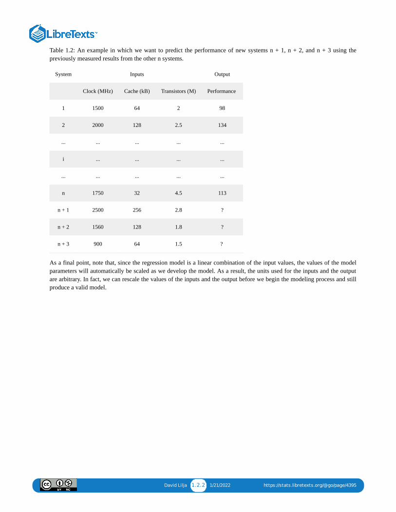
Table 1.2: An example in which we want to predict the performance of new systems n + 1, n + 2, and n + 3 using thepreviously measured results from the other n systems.

System Inputs Output

Clock (MHz) Cache (kB) Transistors (M) Performance

1 1500 64 2 98

2 2000 128 2.5 134

... ... ... ... ...

i ... ... ... ...

... ... ... ... ...

n 1750 32 4.5 113

n + 1 2500 256 2.8 ?

n + 2 1560 128 1.8 ?

n + 3 900 64 1.5 ?

As a final point, note that, since the regression model is a linear combination of the input values, the values of the modelparameters will automatically be scaled as we develop the model. As a result, the units used for the inputs and the outputare arbitrary. In fact, we can rescale the values of the inputs and the output before we begin the modeling process and stillproduce a valid model.

David Lilja 1.3.1 2/4/2022 https://stats.libretexts.org/@go/page/4396

1.3: What is R?R is a computer language developed specifically for statistical computing. It is actually more than that, though. R providesa complete environment for interacting with your data. You can directly use the functions that are provided in theenvironment to process your data without writing a complete program. You also can write your own programs to performoperations that do not have built-in functions, or to repeat the same task multiple times, for instance.

R is an object-oriented language that uses vectors and matrices as its basic operands. This feature makes it quite usefulfor working on large sets of data using only a few lines of code. The R environment also provides excellent graphical toolsfor producing complex plots relatively easily. And, perhaps best of all, it is free. It is an open source project developed bymany volunteers. You can learn more about the history of R, and download a copy to your own computer, from the RProject web site [13].

As an example of using R, here is a copy of a simple interaction with the R environment. > x x [1] 2 4 6 8 10 12 14 16 >mean(x) [1] 9 > var(x) [1] 24 > In this listing, the “>” character indicates that R is waiting for input. The line x <- c(2, 4, 6,8, 10, 12, 14, 16) concatenates all of the values in the argument into a vector and assigns that vector to the variable x.Simply typing x by itself causes R to print the contents of the vector. Note that R treats vectors as a matrix with a singlerow. Thus, the “[1]” preceding the values is R’s notation to show that this is the first row of the matrix x. The next line,mean(x), calls a function in R that computes the arithmetic mean of the input vector, x. The function var(x) computes thecorresponding variance.

This book will not make you an expert in programming using the R computer language. Developing good regressionmodels is an interactive process that requires you to dig in and play around with your data and your models. Thus, I ammore interested in using R as a computing environment for doing statistical analysis than as a programming language.Instead of teaching you the language’s syntax and semantics directly, this tutorial will introduce what you need to knowabout R as you need it to perform the specific steps to develop a regression model. You should already have someprogramming expertise so that you can follow the examples in the remainder of the book. However, you do not need to bean expert programmer.

David Lilja 1.4.1 1/7/2022 https://stats.libretexts.org/@go/page/4397

1.4: What's Next?Before beginning any sort of data analysis, you need to understand your data. Chapter 2 describes the sample data that willbe used in the examples throughout this tutorial, and how to read this data into the R environment. Chapter 3 introduces thesimplest regression model consisting of a single independent variable. The process used to develop a more complexregression model with multiple independent input variables is explained in Chapter 4. Chapter 5 then shows how to usethis multi-factor regression model to predict the system response when given new input data. Chapter 6 explains in moredetail the routines used to read a file containing your data into the R environment. The process used to develop a multi-factor regression model is summarized in Chapter 7 along with some suggestions for further reading. Finally, Chapter 8provides some experiments you might want to try to expand your understanding of the modeling process.

1 2/18/2022

CHAPTER OVERVIEW2: UNDERSTAND YOUR DATA

Good data are the basis of any sort of regression model, because we use this data to actually construct the model. If the data is flawed, themodel will be flawed. It is the old maxim of garbage in, garbage out. Thus, the first step in regression modeling is to ensure that your data isreliable. There is no universal approach to verifying the quality of your data, unfortunately. If you collect it yourself, you at least have theadvantage of knowing its provenance. If you obtain your data from somewhere else, though, you depend on the source to ensure data quality.Your job then becomes verifying your source’s reliability and correctness as much as possible.

2.1: MISSING VALUESAny large collection of data is probably incomplete. That is, it is likely that there will be cells without values in your data table. Thesemissing values may be the result of an error, such as the experimenter simply forgetting to fill in a particular entry. They also could bemissing because that particular system configuration did not have that parameter available. Fortunately, R is designed to gracefully handlemissing values.

2.2: SANITY CHECKING AND DATA CLEANING2.3: THE EXAMPLE DATA2.4: DATA FRAMESThe fundamental object used for storing tables of data in R is called a data frame. We can think of a data frame as a way of organizing datainto a large table with a row for each system measured and a column for each parameter. An interesting and useful feature of R is that allthe columns in a data frame do not need to be the same data type. Some columns may consist of numerical data, for instance, while othercolumns contain textual data.

2.5: ACCESSING A DATA FRAME

David Lilja 2.1.1 1/6/2022 https://stats.libretexts.org/@go/page/4402

2.1: Missing ValuesAny large collection of data is probably incomplete. That is, it is likely that there will be cells without values in your datatable. These missing values may be the result of an error, such as the experimenter simply forgetting to fill in a particularentry. They also could be missing because that particular system configuration did not have that parameter available. Forexample, not every processor tested in our example data had an L2 cache. Fortunately, R is designed to gracefully handlemissing values. R uses the notation NA to indicate that the corresponding value is not available.

Most of the functions in R have been written to appropriately ignore NA values and still compute the desired result.Sometimes, however, you must explicitly tell the function to ignore the NA values. For example, calling the mean()function with an input vector that contains NA values causes it to return NA as the result. To compute the mean of theinput vector while ignoring the NA values, you must explicitly tell the function to remove the NA values using mean(x,na.rm=TRUE).

David Lilja 2.2.1 1/7/2022 https://stats.libretexts.org/@go/page/4403

2.2: Sanity Checking and Data CleaningRegardless of where you obtain your data, it is important to do some sanity checks to ensure that nothing is drasticallyflawed. For instance, you can check the minimum and maximum values of key input parameters (i.e., columns) of yourdata to see if anything looks obviously wrong. One of the exercises in Chapter 8 encourages you explore other approachesfor verifying your data. R also provides good plotting functions to quickly obtain a visual indication of some of the keyrelationships in your data set. We will see some examples of these functions in Section 3.1.

If you discover obvious errors or flaws in your data, you may have to eliminate portions of that data. For instance, you mayfind that the performance reported for a few system configurations is hundreds of times larger than that of all of the othersystems tested. Although it is possible that this data is correct, it seems more likely that whoever recorded the data simplymade a transcription error. You may decide that you should delete those results from your data. It is important, though, notto throw out data that looks strange without good justification. Sometimes the most interesting conclusions come from datathat on first glance appeared flawed, but was actually hiding an interesting and unsuspected phenomenon. This process ofchecking your data and putting it into the proper format is often called data cleaning.

It also is always appropriate to use your knowledge of the system and the relationships between the inputs and the outputto inform your model building. For instance, from our experience, we expect that the clock rate will be a key parameter inany regression model of computer systems performance that we construct. Consequently, we will want to make sure thatour models include the clock parameter. If the modeling methodology suggests that the clock is not important in the model,then using the methodology is probably an error. We additionally may have deeper insights into the physical system thatsuggest how we should proceed in developing a model. We will see a specific example of applying our insights about theeffect of caches on system performance when we begin constructing more complex models in Chapter 4.

These types of sanity checks help you feel more comfortable that your data is valid. However, keep in mind that it isimpossible to prove that your data is flawless. As a result, you should always look at the results of any regression modelingexercise with a healthy dose of skepticism and think carefully about whether or not the results make sense. Trust yourintuition. If the results don’t feel right, there is quite possibly a problem lurking somewhere in the data or in your analysis.

David Lilja 2.3.1 1/14/2022 https://stats.libretexts.org/@go/page/4404

2.3: The Example DataI obtained the input data used for developing the regression models in the subsequent chapters from the publicly availableCPU DB database [2]. This database contains design characteristics and measured performance results for a largecollection of commercial processors. The data was collected over many years and is nicely organized using a commonformat and a standardized set of parameters. The particular version of the database used in this book contains informationon 1,525 processors.

Many of the database’s parameters (columns) are useful in understanding and comparing the performance of the variousprocessors. Not all of these parameters will be useful as predictors in the regression models, however. For instance, someof the parameters, such as the column labeled Instruction set width, are not available for many of the processors. Others,such as the Processor family, are common among several processors and do not provide useful information fordistinguishing among them. As a result, we can eliminate these columns as possible predictors when we develop theregression model.

On the other hand, based on our knowledge of processor design, we know that the clock frequency has a large effect onperformance. It also seems likely that the parallelism-related parameters, specifically, the number of threads and cores,could have a significant effect on performance, so we will keep these parameters available for possible inclusion in theregression model.

Technology-related parameters are those that are directly determined by the particular fabrication technology used to buildthe processor. The number of transistors and the die size are rough indicators of the size and complexity of the processor’slogic. The feature size, channel length, and FO4 (fanout-of-four) delay are related to gate delays in the processor’s logic.Because these parameters both have a direct effect on how much processing can be done per clock cycle and effect thecritical path delays, at least some of these parameters could be important in a regression model that describes performance.

Finally, the memory-related parameters recorded in the database are the separate L1 instruction and data cache sizes, andthe unified L2 and L3 cache sizes. Because memory delays are critical to a processor’s performance, all of these memory-related parameters have the potential for being important in the regression models.

The reported performance metric is the score obtained from the SPEC CPU integer and floating-point benchmarkprograms from 1992, 1995, 2000, and 2006 [6–8]. This performance result will be the regression model’s output. Note thatperformance results are not available for every processor running every benchmark. Most of the processors haveperformance results for only those benchmark sets that were current when the processor was introduced into the market.Thus, although there are more than 1,500 lines in the database representing more than 1,500 unique processorconfigurations, a much

David Lilja 2.4.1 1/6/2022 https://stats.libretexts.org/@go/page/4405

2.4: Data FramesThe fundamental object used for storing tables of data in R is called a data frame. We can think of a data frame as a way oforganizing data into a large table with a row for each system measured and a column for each parameter. An interestingand useful feature of R is that all the columns in a data frame do not need to be the same data type. Some columns mayconsist of numerical data, for instance, while other columns contain textual data. This feature is quite useful whenmanipulating large, heterogeneous data files.

To access the CPU DB data, we first must read it into the R environment. R has built-in functions for reading data directlyfrom files in the csv (comma separated values) format and for organizing the data into data frames. The specifics of thisreading process can get a little messy, depending on how the data is organized in the file. We will defer the specifics ofreading the CPU DB file into R until Chapter 6. For now, we will use a function called extract_data(), which wasspecifically written for reading the CPU DB file.

To use this function, copy both the all-data.csv and read-data.R files into a directory on your computer (you can downloadboth of these files from this book’s web site shown on p. ii). Then start the R environment and set the local directory in Rto be this directory using the File -> Change dir pull-down menu. Then use the File -> Source R code pull-down menu toread the read-data.R file into R. When the R code in this file completes, you should have six new data frames in your Renvironment workspace: int92.dat, fp92.dat, int95.dat, fp95.dat, int00.dat, fp00.dat, int06.dat, and fp06.dat.

The data frame int92.dat contains the data from the CPU DB database for all of the processors for which performanceresults were available for the SPEC Integer 1992 (Int1992) benchmark program. Similarly, fp92.dat contains the data forthe processors that executed the Floating-Point 1992 (Fp1992) benchmarks, and so on. I use the .dat suffix to show that thecorresponding variable name is a data frame.

Simply typing the name of the data frame will cause R to print the entire table. For example, here are the first few linesprinted after I type int92.dat, truncated to fit within the page: nperf perf clock threads cores ... 1 9.662070 68.60000 100 11 ... 2 7.996196 63.10000 125 1 1 ... 3 16.363872 90.72647 166 1 1 ... 4 13.720745 82.00000 175 1 1 ... ... The first row isthe header, which shows the name of each column. Each subsequent row contains the data corresponding to an individualprocessor. The first column is the index number assigned to the processor whose data is in that row. The next columns arethe specific values recorded for that parameter for each processor. The function head(int92.dat) prints out just the headerand the first few rows of the corresponding data frame. It gives you a quick glance at the data frame when you interactwith your data.

Table 2.1shows the complete list of column names available in these data frames. Note that the column names are listedvertically in this table, simply to make them fit on the page.

Table 2.1: The names and definitions of the columns in the data frames containing the data from CPU DB.

Column number Column name Definition

1 (blank) Processor index number

2 nperf Normalized performance

3 perf SPEC performance

4 clock Clock frequency (MHz)

5 threads Number of hardware threads available

6 cores Number of hardware cores available

7 TDP Thermal design power

David Lilja 2.4.2 1/6/2022 https://stats.libretexts.org/@go/page/4405

8 transistors Number of transistors on the chip (M)

9 dieSize The size of the chip

10 voltage Nominal operating voltage

11 featureSize Fabrication feature size

12 channel Fabrication channel size

13 FO4delay Fan-out-four delay

14 L1icache Level 1 instruction cache size

15 L1dcache Level 1 data cache size

16 L2cache Level 2 cache size

17 L3cache Level 3 cache size

David Lilja 2.5.1 2/11/2022 https://stats.libretexts.org/@go/page/4406

2.5: Accessing a Data FrameWe access the individual elements in a data frame using square brackets to identify a specific cell. For instance, thefollowing accesses the data in the cell in row 15, column 12:

> int92.dat[15,12]

[1] 180

We can also access cells by name by putting quotes around the name:

> int92.dat["71","perf"]

[1] 105.1

This expression returns the data in the row labeled 71 and the column labeled perf . Note that this is not row 71, butrather the row that contains the data for the processor whose name is 71 .

We can access an entire column by leaving the first parameter in the square brackets empty. For instance, the followingprints the value in every row for the column labeled clock :

> int92.dat[,"clock"]

[1] 100 125 166 175 190 ...

Similarly, this expression prints the values in all of the columns for row 36:

> int92.dat[36,]

nperf perf clock threads cores ...

36 13.07378 79.86399 80 1 1 ...

The functions nrow() and ncol() return the number of rows and columns, respectively, in the data frame:

> nrow(int92.dat)

[1] 78

> ncol(int92.dat)

[1] 16

Because R functions can typically operate on a vector of any length, we can use built-in functions to quickly computesome useful results. For example, the following expressions compute the minimum, maximum, mean, and standarddeviation of the perf column in the int92.dat data frame:

> min(int92.dat[,"perf"])

[1] 36.7

> max(int92.dat[,"perf"])

[1] 366.857

> mean(int92.dat[,"perf"])

[1] 124.2859

> sd(int92.dat[,"perf"])

[1] 78.0974

This square-bracket notation can become cumbersome when you do a substantial amount of interactive computation withinthe R environment. R provides an alternative notation using the $ symbol to more easily access a column. Repeating theprevious example using this notation:

David Lilja 2.5.2 2/11/2022 https://stats.libretexts.org/@go/page/4406

> min(int92.dat$perf)

[1] 36.7

> max(int92.dat$perf)

[1] 366.857

> mean(int92.dat$perf)

[1] 124.2859

> sd(int92.dat$perf)

[1] 78.0974

This notation says to use the data in the column named perf from the data frame named int92.dat . We canmake yet a further simplification using the attach function. This function makes the corresponding data frame localto the current workspace, thereby eliminating the need to use the potentially awkward $ or square-bracket indexingnotation. The following example shows how this works:

> attach(int92.dat)

> min(perf)

[1] 36.7

> max(perf)

[1] 366.857

> mean(perf)

[1] 124.2859

> sd(perf)

[1] 78.0974

To change to a different data frame within your local workspace, you must first detach the current data frame:

> detach(int92.dat)

> attach(fp00.dat)

> min(perf)

[1] 87.54153

> max(perf)

[1] 3369

> mean(perf)

[1] 1217.282

> sd(perf)

[1] 787.4139

Now that we have the necessary data available in the R environment, and some understanding of how to access andmanipulate this data, we are ready to generate our first regression model.

1 2/18/2022

CHAPTER OVERVIEW3: ONE-FACTOR REGRESSIONThe simplest linear regression model finds the relationship between one input variable, which is called the predictor variable, and the output,which is called the system’s response. This type of model is known as a one-factor linear regression. To demonstrate the regression-modelingprocess, we will begin developing a one-factor model for the SPEC Integer 2000 (Int2000) benchmark results reported in the CPU DB dataset.

3.1: VISUALIZE THE DATA3.2: THE LINEAR MODEL FUNCTION3.3: EVALUATING THE QUALITY OF THE MODEL3.4: RESIDUAL ANALYSIS

David Lilja 3.1.1 1/21/2022 https://stats.libretexts.org/@go/page/4409

3.1: Visualize the DataThe first step in this one-factor modeling process is to determine whether or not it looks as though a linear relationshipexists between the predictor and the output value. From our understanding of computer system design that is, fromour domain-specific knowledge we know that the clock frequency strongly influences a computer system’s performance.Consequently, we must look for a roughly linear relationship between the processor’s performance and its clock frequency.Fortunately, R provides powerful and flexible plotting functions that let us visualize this type relationship quite easily.

This R function call:

generates the plot shown in Figure 3.1. The first parameter in this function call is the value we will plot on the x-axis. Inthis case, we will plot the clock values from the int00.dat data frame as the independent variable

Figure 3.1: A scatter plot of the performance of the processors that were tested using the Int2000 benchmark versus theclock frequency.

on the x-axis. The dependent variable is the perf column from int00.dat , which we plot on the y-axis. The functionargument main="Int2000" provides a title for the plot, while xlab="Clock" and ylab="Performance" provide labels for the xand y-axes, respectively.

This figure shows that the performance tends to increase as the clock frequency increases, as we expected. If wesuperimpose a straight line on this scatter plot, we see that the relationship between the predictor (the clock frequency) andthe output (the performance) is roughly linear. It is not perfectly linear, however. As the clock frequency increases, we seea larger spread in performance values. Our next step is to develop a regression model that will help us quantify the degreeof linearity in the relationship between the output and the predictor.

> plot(int00.dat[,"clock"],int00.dat[,"perf"], main="Int2000", xlab="Clock",

David Lilja 3.2.1 2/11/2022 https://stats.libretexts.org/@go/page/4410

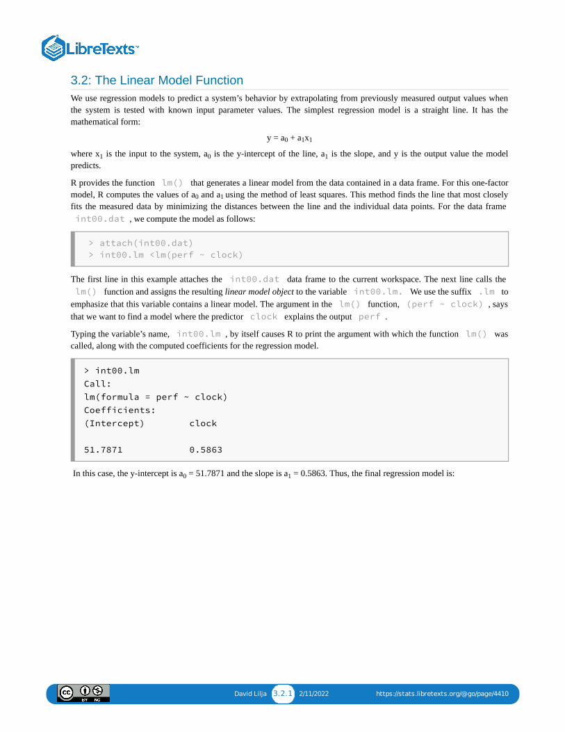
3.2: The Linear Model FunctionWe use regression models to predict a system’s behavior by extrapolating from previously measured output values whenthe system is tested with known input parameter values. The simplest regression model is a straight line. It has themathematical form:

y = a + a x

where x is the input to the system, a is the y-intercept of the line, a is the slope, and y is the output value the modelpredicts.

R provides the function lm() that generates a linear model from the data contained in a data frame. For this one-factormodel, R computes the values of a and a using the method of least squares. This method finds the line that most closelyfits the measured data by minimizing the distances between the line and the individual data points. For the data frame int00.dat , we compute the model as follows:

> attach(int00.dat)

> int00.lm <lm(perf ~ clock)

The first line in this example attaches the int00.dat data frame to the current workspace. The next line calls the lm() function and assigns the resulting linear model object to the variable int00.lm. We use the suffix .lm to

emphasize that this variable contains a linear model. The argument in the lm() function, (perf ~ clock) , saysthat we want to find a model where the predictor clock explains the output perf .

Typing the variable’s name, int00.lm , by itself causes R to print the argument with which the function lm() wascalled, along with the computed coefficients for the regression model.

> int00.lm

Call:

lm(formula = perf ~ clock)

Coefficients:

(Intercept) clock

51.7871 0.5863

In this case, the y-intercept is a = 51.7871 and the slope is a = 0.5863. Thus, the final regression model is:

0 1 1

1 0 1

0 1

0 1

David Lilja 3.2.2 2/11/2022 https://stats.libretexts.org/@go/page/4410

Figure 3.2: The one-factor linear regression model superimposed on the data from Figure 3.1.

perf = 51.7871 + 0.5863 ∗ clock.

The following code plots the original data along with the fitted line, as shown in Figure 3.2. The function abline() isshort for (a,b)-line. It plots a line on the active plot window, using the slope and intercept of the linear model given in itsargument.

> plot(clock,perf)

> abline(int00.lm)

David Lilja 3.3.1 2/4/2022 https://stats.libretexts.org/@go/page/4411

3.3: Evaluating the Quality of the ModelThe information we obtain by typing int00.lm shows us the regression model’s basic values, but does not tell usanything about the model’s quality. In fact, there are many different ways to evaluate a regression model’s quality. Many ofthe techniques can be rather technical, and the details of them are beyond the scope of this tutorial. However, the function summary() extracts some additional information that we can use to determine how well the data fit the resulting

model. When called with the model object int00.lm as the argument, summary() produces the followinginformation:

> summary(int00.lm)

Call:

lm(formula = perf ~ clock)

Residuals:

Min 1Q Median 3Q Max

-634.61 -276.17 -30.83 75.38 1299.52

Coefficients:

Estimate Std. Error t value Pr(>|t|)

(Intercept) 51.78709 53.31513 0.971 0.332

clock 0.58635 0.02697 21.741 <2e-16 ***

---

Signif. codes: 0 ‘***’ 0.001 ‘**’ 0.01 ‘*’0.05 ‘.’ 0.1 ‘ ’ 1

Residual standard error: 396.1 on 254 degrees of freedom

Multiple R-squared: 0.6505, Adjusted R-squared: 0.6491

F-statistic: 472.7 on 1 and 254 DF, p-value: < 2.2e-16

Let’s examine each of the items presented in this summary in turn.

> summary(int00.lm)

Call:

lm(formula = perf ~ clock)

These first few lines simply repeat how the lm() function was called. It is useful to look at this information to verify thatyou actually called the function as you intended.

Residuals:

Min 1Q Median 3Q Max

-634.61 -276.17 -30.83 75.38 1299.52

The residuals are the differences between the actual measured values and the corresponding values on the fitted regressionline. In Figure 3.2, each data point’s residual is the distance that the individual data point is above (positive residual) orbelow (negative residual) the regression line. Min is the minimum residual value, which is the distance from theregression line to the point furthest below the line. Similarly, Max is the distance from the regression line of the pointfurthest above the line. Median is the median value of all of the residuals. The 1Q and 3Q values are the pointsthat mark the first and third quartiles of all the sorted residual values.

How should we interpret these values? If the line is a good fit with the data, we would expect residual values that arenormally distributed around a mean of zero. (Recall that a normal distribution is also called a Gaussian distribution.) Thisdistribution implies that there is a decreasing probability of finding residual values as we move further away from themean. That is, a good model’s residuals should be roughly balanced around and not too far away from the mean of zero.Consequently, when we look at the residual values reported by summary() , a good model would tend to have a

David Lilja 3.3.2 2/4/2022 https://stats.libretexts.org/@go/page/4411

median value near zero, minimum and maximum values of roughly the same magnitude, and first and third quartile valuesof roughly the same magnitude. For this model, the residual values are not too far off what we would expect for Gaussian-distributed numbers. In Section 3.4, we present a simple visual test to determine whether the residuals appear to follow anormal distribution.

Coefficients:

Estimate Std. Error t value Pr(>|t|)

(Intercept) 51.78709 53.31513 0.971 0.332

clock 0.58635 0.02697 21.741 <2e-16 ***

---

Signif. codes: 0 ‘***’ 0.001 ‘**’ 0.01 ‘*’ 0.05 ‘.’ 0.1 ‘ ’ 1

This portion of the output shows the estimated coefficient values. These values are simply the fitted regression modelvalues from Equation 3.2. The Std. Error column shows the statistical standard error for each of the coefficients.For a good model, we typically would like to see a standard error that is at least five to ten times smaller than thecorresponding coefficient. For example, the standard error for clock is 21.7 times smaller than the coefficient value(0.58635/0.02697 = 21.7). This large ratio means that there is relatively little variability in the slope estimate, a . Thestandard error for the intercept, a , is 53.31513, which is roughly the same as the estimated value of 51.78709 for thiscoefficient. These similar values suggest that the estimate of this coefficient for this model can vary significantly.

The last column, labeled Pr(>|t|) , shows the probability that the corresponding coefficient is not relevant in themodel. This value is also known as the significance or p-value of the coefficient. In this example, the probability that clock is not relevant in this model is 2 × 10−16 a tiny value. The probability that the intercept is not relevant is 0.332,

or about a one-inthree chance that this specific intercept value is not relevant to the model. There is an intercept, of course,but we are again seeing indications that the model is not predicting this value very well.

The symbols printed to the right in this summary that is, the asterisks, periods, or spaces are intended to give a quick visualcheck of the coefficients’ significance. The line labeled Signif. codes: gives these symbols’ meanings. Threeasterisks (***) means 0 < p ≤ 0.001, two asterisks (**) means 0.001 < p ≤ 0.01, and so on.

R uses the column labeled t value to compute the p-values and the corresponding significance symbols. Youprobably will not use these values directly when you evaluate your model’s quality, so we will ignore this column for now.

Residual standard error: 396.1 on 254 degrees of freedom

Multiple R-squared: 0.6505, Adjusted R-squared: 0.6491

F-statistic: 472.7 on 1 and 254 DF, p-value: < 2.2e-16

These final few lines in the output provide some statistical information about the quality of the regression model’s fit to thedata. The Residual standard error is a measure of the total variation in the residual values. If the residuals aredistributed normally, the first and third quantiles of the previous residuals should be about 1.5 times this standard error .

The number of degrees of freedom is the total number of measurements or observations used to generate themodel, minus the number of coefficients in the model. This example had 256 unique rows in the data frame, correspondingto 256 independent measurements. We used this data to produce a regression model with two coefficients: the slope andthe intercept. Thus, we are left with (256 2 = 254) degrees of freedom.

The Multiple R-squared value is a number between 0 and 1. It is a statistical measure of how well the modeldescribes the measured data. We compute it by dividing the total variation that the model explains by the data’s totalvariation. Multiplying this value by 100 gives a value that we can interpret as a percentage between 0 and 100. Thereported R of 0.6505 for this model means that the model explains 65.05 percent of the data’s variation. Random chanceand measurement errors creep in, so the model will never explain all data variation. Consequently, you should not everexpect an R value of exactly one. In general, values of R2 that are closer to one indicate a better-fitting model. However, a

1

0

2

2

David Lilja 3.3.3 2/4/2022 https://stats.libretexts.org/@go/page/4411

good model does not necessarily require a large R value. It may still accurately predict future observations, even with asmall R value.

The Adjusted R-squared value is the R value modified to take into account the number of predictors used in themodel. The adjusted R is always smaller than the R value. We will discuss the meaining of the adjusted R in Chapter 4,when we present regression models that use more than one predictor.

The final line shows the F-statistic . This value compares the current model to a model that has one fewerparameters. Because the one-factor model already has only a single parameter, this test is not particularly useful in thiscase. It is an interesting statistic for the multi-factor models, however, as we will discuss later.

2

2

2

2 2 2

David Lilja 3.4.1 2/4/2022 https://stats.libretexts.org/@go/page/4412

3.4: Residual AnalysisThe summary() function provides a substantial amount of information to help us evaluate a regression model’s fit tothe data used to develop that model. To dig deeper into the model’s quality, we can analyze some additional informationabout the observed values compared to the values that the model predicts. In particular, residual analysis examines theseresidual values to see what they can tell us about the model’s quality.

Recall that the residual value is the difference between the actual measured value stored in the data frame and the valuethat the fitted regression line predicts for that corresponding data point. Residual values greater than zero mean that theregression model predicted a value that was too small compared to the actual measured value, and negative values indicatethat the regression model predicted a value that was too large. A model that fits the data well would tend to over-predict asoften as it under-predicts. Thus, if we plot the residual values, we would expect to see them distributed uniformly aroundzero for a well-fitted model.

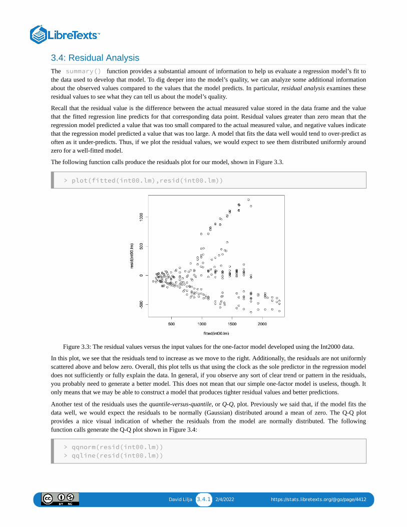
The following function calls produce the residuals plot for our model, shown in Figure 3.3.

> plot(fitted(int00.lm),resid(int00.lm))

Figure 3.3: The residual values versus the input values for the one-factor model developed using the Int2000 data.

In this plot, we see that the residuals tend to increase as we move to the right. Additionally, the residuals are not uniformlyscattered above and below zero. Overall, this plot tells us that using the clock as the sole predictor in the regression modeldoes not sufficiently or fully explain the data. In general, if you observe any sort of clear trend or pattern in the residuals,you probably need to generate a better model. This does not mean that our simple one-factor model is useless, though. Itonly means that we may be able to construct a model that produces tighter residual values and better predictions.

Another test of the residuals uses the quantile-versus-quantile, or Q-Q, plot. Previously we said that, if the model fits thedata well, we would expect the residuals to be normally (Gaussian) distributed around a mean of zero. The Q-Q plotprovides a nice visual indication of whether the residuals from the model are normally distributed. The followingfunction calls generate the Q-Q plot shown in Figure 3.4:

> qqnorm(resid(int00.lm))

> qqline(resid(int00.lm))

David Lilja 3.4.2 2/4/2022 https://stats.libretexts.org/@go/page/4412

Figure 3.4: The Q-Q plot for the one-factor model developed using the Int2000 data.

If the residuals were normally distributed, we would expect the points plotted in this figure to follow a straight line. Withour model, though, we see that the two ends diverge significantly from that line. This behavior indicates that the residualsare not normally distributed. In fact, this plot suggests that the distribution’s tails are “heavier” than what we would expectfrom a normal distribution. This test further confirms that using only the clock as a predictor in the model is insufficient toexplain the data.

Our next step is to learn to develop regression models with multiple input factors. Perhaps we will find a more complexmodel that is better able to explain the data.

1 2/18/2022

CHAPTER OVERVIEW4: MULTI-FACTOR REGRESSION

A multi-factor regression model is a generalization of the simple one- factor regression model discussed in Chapter 3. It has n factors withthe form:

y = a0 + a1x1 + a2x2 + ...anxn,

where the xi values are the inputs to the system, the ai coefficients are the model parameters computed from the measured data, and y is theoutput value predicted by the model. Everything we learned in Chapter 3 for one- factor models also applies to the multi-factor models. Todevelop this type of multi-factor regression model, we must also learn how to select specific predictors to include in the model

4.1: VISUALIZING THE RELATIONSHIPS IN THE DATA4.2: IDENTIFYING POTENTIAL PREDICTORS4.3: THE BACKWARD ELIMINATION PROCESS4.4: AN EXAMPLE OF THE BACKWARD ELIMINATION PROCESS4.5: RESIDUAL ANALYSIS4.6: WHEN THINGS GO WRONG

David Lilja 4.1.1 2/11/2022 https://stats.libretexts.org/@go/page/4416

4.1: Visualizing the Relationships in the DataBefore beginning model development, it is useful to get a visual sense of the relationships within the data. We can do thiseasily with the following function call:

> pairs(int00.dat, gap=0.5)

The pairs() function produces the plot shown in Figure 4.1. This plot provides a pairwise comparison of all the datain the  int00.dat data frame. The gap parameter in the function call controls the spacing between the individualplots. Set it to zero to eliminate any space between plots.

As an example of how to read this plot, locate the box near the upper left corner labeled perf . This is the value of theperformance measured for the int00.dat data set. The box immediately to the right of this one is a scatter

Figure 4.1: All of the pairwise comparisons for the Int2000 data frame.

plot, with perf data on the vertical axis and clock data on the horizontal axis. This is the same information wepreviously plotted in Figure 3.1. By scanning through these plots, we can see any obviously significant relationshipsbetween the variables. For example, we quickly observe that there is a somewhat proportional relationship between perf and clock . Scanning down the perf column, we also see that there might be a weakly inverse

relationship between perf and featureSize .

Notice that there is a perfect linear correlation between perf and nperf . This relationship occurs because nperf is a simple rescaling of perf . The reported benchmark performance values in the database that is, the perf values use different scales for different benchmarks. To directly compare the values that our models will predict,

it is useful to rescale perf to the range [0,100]. Do this quite easily, using this R code:

max_perf = max(perf)

min_perf = min(perf)

range = max_perf min_perf

nperf = 100 * (perf min_perf) / range

Note that this rescaling has no effect on the models we will develop, because it is a linear transformation of perf . Forconvenience and consistency, we use nperf in the remainder of this tutorial.

David Lilja 4.2.1 1/21/2022 https://stats.libretexts.org/@go/page/4417

4.2: Identifying Potential PredictorsThe first step in developing the multi-factor regression model is to identify all possible predictors that we could include inthe model. To the novice model developer, it may seem that we should include all factors available in the data aspredictors, because more information is likely to be better than not enough information. However, a good regression modelexplains the relationship between a system’s inputs and output as simply as possible. Thus, we should use the smallestnumber of predictors necessary to provide good predictions. Furthermore, using too many or redundant predictors buildsthe random noise in the data into the model. In this situation, we obtain an over-fitted model that is very good at predictingthe outputs from the specific input data set used to train the model. It does not accurately model the overall system’sresponse, though, and it will not appropriately predict the system output for a broader range of inputs than those on whichit was trained. Redundant or unnecessary predictors also can lead to numerical instabilities when computing thecoefficients.

We must find a balance between including too few and too many predictors. A model with too few predictors can producebiased predictions. On the other hand, adding more predictors to the model will always cause the R value to increase. Thiscan confuse you into thinking that the additional predictors generated a better model. In some cases, adding a predictor willimprove the model, so the increase in the R value makes sense. In some cases, however, the R value increases simplybecause we’ve better modeled the random noise.

The adjusted R attempts to compensate for the regular R ’s behavior by changing the R value according to the number ofpredictors in the model. This adjustment helps us determine whether adding a predictor improves the fit of the model, orwhether it is simply modeling the noise better. It is computed as:

where n is the number of observations and m is the number of predictors in the model. If adding a new predictor to themodel increases the previous model’s R value by more than we would expect from random fluctuations, then theadjusted R will increase. Conversely, it will decrease if removing a predictor decreases the R by more than we wouldexpect due to random variations. Recall that the goal is to use as few predictors as possible, while still producing a modelthat explains the data well.

Because we do not know a priori which input parameters will be useful predictors, it seems reasonable to start with all ofthe columns available in the measured data as the set of potential predictors. We listed all of the column names inTable 2.1. Before we throw all these columns into the modeling process, though, we need to step back and consider whatwe know about the underlying system, to help us find any parameters that we should obviously exclude from the start.

There are two output columns: perf and nperf . The regression model can have only one output, however, so wemust choose only one column to use in our model development process. As discussed in Section 4.1, nperf is a lineartransformation of perf that shifts the output range to be between 0 and 100. This range is useful for quickly obtaininga sense of future predictions’ quality, so we decide to use nperf as our model’s output and ignore the perf column.

Almost all the remaining possible predictors appear potentially useful in our model, so we keep them available as potentialpredictors for now. The only exception is TDP . The name of this factor, thermal design power, does not clearly indicatewhether this could be a useful predictor in our model, so we must do a little additional research to understand it better. Wediscover [10] that thermal design power is “the average amount of power in watts that a cooling system must dissipate.Also called the ‘thermal guideline’ or ‘thermal design point,’ the TDP is provided by the chip manufacturer to the systemvendor, who is expected to build a case that accommodates the chip’s thermal requirements.” From this definition, weconclude that TDP is not really a parameter that will directly affect performance. Rather, it is a specification provided bythe processor’s manufacturer to ensure that the system designer includes adequate cooling capability in the final product.Thus, we decide not to include TDP as a potential predictor in the regression model.

In addition to excluding some apparently unhelpful factors (such as TDP) at the beginning of the model developmentprocess, we also should consider whether we should include any additional parameters. For example, the terms in aregression model add linearly to produce the predicted output. However, the individual terms themselves can be nonlinear,such as a x ,where m does not have to be equal to one.This flexibility lets us include additional powers of the

2

2 2

2 2 2

  = 1 − (1 − )R2adjusted

n−1n−m

R2

2

2 2

i im

David Lilja 4.2.2 1/21/2022 https://stats.libretexts.org/@go/page/4417

individual factors. We should include these non-linear terms, though, only if we have some physical reason to suspect thatthe output could be a nonlinear function of a particular input.

For example, we know from our prior experience modeling processor performance that empirical studies have suggestedthat cache miss rates are roughly proportional to the square root of the cache size [5]. Consequently, we will include termsfor the square root (m = 1/2) of each cache size as possible predictors. We must also include first-degree terms (m = 1) ofeach cache size as possible predictors. Finally, we notice that only a few of the entries in the int00.dat data frameinclude values for the L3 cache, so we decide to exclude the L3 cache size as a potential predictor. Exploiting this type ofdomain-specific knowledge when selecting predictors ultimately can help produce better models than blindly applying themodel development process.

The final list of potential predictors that we will make available for the model development process is shown in Table 4.1.

Table 4.1: The list of potential predictors to be used in the model development process.

David Lilja 4.3.1 1/6/2022 https://stats.libretexts.org/@go/page/4418

4.3: The Backward Elimination ProcessWe are finally ready to develop the multi-factor linear regression model for the int00.dat data set. As mentioned inthe previous section, we must find the right balance in the number of predictors that we use in our model. Too manypredictors will train our model to follow the data’s random variations (noise) too closely. Too few predictors will produce amodel that may not be as accurate at predicting future values as a model with more predictors.

We will use a process called backward elimination [1] to help decide which predictors to keep in our model and which toexclude. In backward elimination, we start with all possible predictors and then use lm() to compute the model. Weuse the summary() function to find each predictor’s significance level. The predictor with the least significance hasthe largest p-value. If this value is larger than our predetermined significance threshold, we remove that predictor from themodel and start over. A typical threshold for keeping predictors in a model is p = 0.05, meaning that there is at least a 95percent chance that the predictor is meaningful. A threshold of p = 0.10 also is not unusual. We repeat this process until thesignificance levels of all of the predictors remaining in the model are below our threshold.

All of these approaches have their advantages and disadvantages, their supporters and detractors. I prefer the backwardelimination process because it is usually straightforward to determine which factor we should drop at each step of theprocess. Determining which factor to try at each step is more difficult with forward selection. Backward elimination has afurther advantage, in that several factors together may have better predictive power than any subset of these factors. As aresult, the backward elimination process is more likely to include these factors as a group in the final model than is theforward selection process.

The automated procedures have a very strong allure because, as technologically savvy individuals, we tend to believe thatthis type of automated process will likely test a broader range of possible predictor combinations than we could testmanually. However, these automated procedures lack intuitive insights into the underlying physical nature of the systembeing modeled. Intuition can help us answer the question of whether this is a reasonable model to construct in the firstplace.

As you develop your models, continually ask yourself whether the model “makes sense.” Does it make sense thatfactor i is included but factor j is excluded? Is there a physical explanation to support the inclusion or exclusion of anypotential factor? Although the automated methods can simplify the process, they also make it too easy for you to forget tothink about whether or not each step in the modeling process makes sense.

David Lilja 4.4.1 1/14/2022 https://stats.libretexts.org/@go/page/4419

4.4: An Example of the Backward Elimination ProcessWe previously identified the list of possible predictors that we can include in our models, shown in Table 4.1. We start thebackward elimination process by putting all these potential predictors into a model for the int00.dat data frameusing the  lm() function.

> int00.lm <lm(nperf ~ clock + threads + cores + transistors +

dieSize + voltage + featureSize + channel + FO4delay + L1icache +

sqrt(L1icache) + L1dcache + sqrt(L1dcache) + L2cache + sqrt(L2cache),

data=int00.dat)

This function call assigns the resulting linear model object to the variable int00.lm . As before, we use the suffix .lm to remind us that this variable is a linear model developed from the data in the corresponding data frame, int00.dat . The arguments in the function call tell  lm() to compute a linear model that explains the output nperf as a function of the predictors separated by the “+” signs. The argument data=int00.dat explicitly

passes to the  lm() function the name of the data frame that should be used when developing this model. This data= argument is not necessary if we attach() the data frame int00.dat to the current workspace.

However, it is useful to explicitly specify the data frame that lm()  should use, to avoid confusion when youmanipulate multiple models simultaneously.

The summary() function gives us a great deal of information about the linear model we just created:

David Lilja 4.4.2 1/14/2022 https://stats.libretexts.org/@go/page/4419

Notice a few things in this summary: First, a quick glance at the residuals shows that they are roughly balanced around amedian of zero, which is what we like to see in our models. Also, notice the line, (179 observations deleted due to missingness ). This tells us that in 179 of the rows in the data

frame that is, in 179 of the processors for which performance results were reported for the Int2000 benchmark some of thevalues in the columns that we would like to use as potential predictors were missing. These NA values caused R toautomatically remove these data rows when computing the linear model.

The total number of observations used in the model equals the number of degrees of freedom remaining 61 in this caseplus the total number of predictors in the model. Finally, notice that the R and adjusted R values are relatively close toone, indicating that the model explains the nperf values well. Recall, however, that these large R values may simplyshow us that the model is good at modeling the noise in the measurements. We must still determine whether we shouldretain all these potential predictors in the model.

To continue developing the model, we apply the backward elimination procedure by identifying the predictor with thelargest p-value that exceeds our predetermined threshold of p = 0.05. This predictor is FO4delay , which has a p-valueof 0.99123. We can use the  update() function to eliminate a given predictor and recompute the model in one step.The notation “.~.” means that  update() should keep the left and right-hand sides of the model the same.By including “ - FO4delay , ”we also tell it to remove that predictor from the model, as shown in the following:

> summary(int00.lm)

Call:

lm(formula = nperf ~ clock + threads + cores + transistors + dieSize +

voltage + featureSize + channel + FO4delay + L1icache + sqrt(L1icache) +

L1dcache + sqrt(L1dcache) + L2cache + sqrt(L2cache), data = int00.dat)

Residuals:

Min 1Q Median 3Q Max

-10.804 -2.702 0.000 2.285 9.809

Coefficients:

Estimate Std. Error t value

(Intercept) -2.108e+01 7.852e+01 -0.268

clock 2.605e-02 1.671e-03 15.594

threads -2.346e+00 2.089e+00 -1.123

cores 2.246e+00 1.782e+00 1.260

transistors -5.580e-03 1.388e-02 -0.402

dieSize 1.021e-02 1.746e-02 0.585

voltage -2.623e+01 7.698e+00 -3.408

freatureSize 3.101e+01 1.122e+02 0.276

channel 9.496e+01 5.945e+02 0.160

FO4delay -1.765e-02 1.600e+00 -0.011

L1icache 1.102e+02 4.206e+01 2.619

sqrt(L1icache) -7.390e+02 2.980e+02 -2.480

L1dcache -1.114e+02 4.019e+01 -2.771

sqrt(L1dcache) 7.492e+02 2.739e+02 2.735

L2cache -9.684e-03 1.745e-03 -5.550

sqrt(L2cache) 1.221e+00 2.425e-01 5.034

---

Signif. codes: 0 ‘***’ 0.001 ‘**’ 0.01 ‘*’ 0.05 ‘.’ 0.1 ‘ ’ 1

Residual standard error: 4.632 on 61 degrees of freedom (179 observations de

Multiple R-squared: 0.9652, Adjusted R-squared: 0.9566 F-statistic: 112.8 on

2 2

2

David Lilja 4.4.3 1/14/2022 https://stats.libretexts.org/@go/page/4419

We repeat this process by removing the next potential predictor with the largest p-value that exceeds our predeterminedthreshold, featureSize . As we repeat this process, we obtain the following sequence of possible models.

Remove featureSize :

> int00.lm <- update(int00.lm, .~. - FO4delay, data = int00.dat) > summary(i

Call:

lm(formula = nperf ~ clock + threads + cores + transistors +

dieSize + voltage + featureSize + channel + L1icache + sqrt(L1icache) +

L1dcache + sqrt(L1dcache) + L2cache + sqrt(L2cache), data = int00.dat)

Residuals:

Min 1Q Median 3Q Max

-10.795 -2.714 0.000 2.283 9.809

Coefficients:

Estimate Std. Error t value Pr(>|t|

(Intercept) -2.088e+01 7.584e+01 -0.275 0.783983

clock 2.604e-02 1.563e-03 16.662 < 2e-16

threads -2.345e+00 2.070e+00 -1.133 0.261641

cores 2.248e+00 1.759e+00 1.278 0.206080

transistors -5.556e-03 1.359e-02 -0.409 0.684020

dieSize 1.013e-02 1.571e-02 0.645 0.521488

voltage -2.626e+01 7.302e+00 -3.596 0.000642

featureSize 3.104e+01 1.113e+02 0.279 0.781232

channel 8.855e+01 1.218e+02 0.727 0.469815

L1icache 1.103e+02 4.041e+01 2.729 0.008257

sqrt(L1icache) -7.398e+02 2.866e+02 -2.581 0.012230

L1dcache -1.115e+02 3.859e+01 -2.889 0.005311

sqrt(L1dcache) 7.500e+02 2.632e+02 2.849 0.005937

L2cache -9.693e-03 1.494e-01 -6.488 1.64e-08

sqrt(L2cache) 1.222e+00 1.975e-01 6.189 5.33e-08

---

Signif. codes: 0 ‘***’ 0.001 ‘**’ 0.01 ‘*’ 0.05 ‘.’ 0.1 ‘ ’ 1

Residual standard error: 4.594 on 62 degrees of freedom (179 observations de

Multiple R-squared: 0.9652, Adjusted R-squared: 0.9573 F-statistic: 122.8 on

> int00.lm <- update(int00.lm, .~. - featureSize, data=int00.dat)

> summary(int00.lm)

Call:

lm(formula = nperf ~ clock + threads + cores + transistors + dieSize +

voltage + channel + L1icache + sqrt(L1icache) + L1dcache + sqrt(L1dcache) +

L2cache + sqrt(L2cache), data = int00.dat)

Residuals:

Min 1Q Median 3Q Max

-10.5548 -2.6442 0.0937 2.2010 10.0264

Coefficients:

Estimate Std. Error t value Pr(>|t|

David Lilja 4.4.4 1/14/2022 https://stats.libretexts.org/@go/page/4419

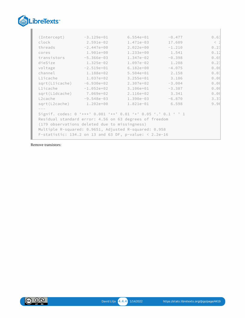
Remove transistors:

(Intercept) -3.129e+01 6.554e+01 -0.477 0.63

clock 2.591e-02 1.471e-03 17.609 < 2

threads -2.447e+00 2.022e+00 -1.210 0.23

cores 1.901e+00 1.233e+00 1.541 0.12

transistors -5.366e-03 1.347e-02 -0.398 0.69

dieSize 1.325e-02 1.097e-02 1.208 0.23

voltage -2.519e+01 6.182e+00 -4.075 0.00

channel 1.188e+02 5.504e+01 2.158 0.03

L1icache 1.037e+02 3.255e+01 3.186 0.00

sqrt(L1icache) -6.930e+02 2.307e+02 -3.004 0.00

L1icache -1.052e+02 3.106e+01 -3.387 0.00

sqrt(L1dcache) 7.069e+02 2.116e+02 3.341 0.00

L2cache -9.548e-03 1.390e-03 -6.870 3.37

sqrt(L2cache) 1.202e+00 1.821e-01 6.598 9.96

---

Signif. codes: 0 ‘***’ 0.001 ‘**’ 0.01 ‘*’ 0.05 ‘.’ 0.1 ‘ ’ 1

Residual standard error: 4.56 on 63 degrees of freedom

(179 observations deleted due to missingness)

Multiple R-squared: 0.9651, Adjusted R-squared: 0.958

F-statistic: 134.2 on 13 and 63 DF, p-value: < 2.2e-16

David Lilja 4.4.5 1/14/2022 https://stats.libretexts.org/@go/page/4419

Remove threads:

> int00.lm <- update(int00.lm, .~. - transistors, data=int00.dat)

> summary(int00.lm)

Call:

lm(formula = nperf ~ clock + threads + cores + dieSize + voltage + channel +

L1icache + sqrt(L1icache) + L1dcache + sqrt(L1dcache) + L2cache + sqrt(L2cac

data = int00.dat)

Residuals:

Min 1Q Median 3Q Max

-9.8861 -3.0801 -0.1871 2.4534 10.4863

Coefficients:

Estimate Std. Error t value Pr(>|t|)

(Intercept) -7.789e+01 4.318e+01 -1.804 0.075745 .

clock 2.566e-02 1.422e-03 18.040 < 2e-16 ***

threads -1.801e+00 1.995e+00 -0.903 0.369794

cores 1.805e+00 1.132e+00 1.595 0.115496

dieSize 1.111e-02 8.807e-03 1.262 0.211407

voltage -2.379e+01 5.734e+00 -4.148 9.64e-05 ***

channel 1.512e+02 3.918e+01 3.861 0.000257 ***

L1icache 8.159e+01 2.006e+01 4.067 0.000128 ***

sqrt(L1icache) -5.386e+02 1.418e+02 -3.798 0.000317 ***

L1dcache -8.422e+01 1.914e+01 -4.401 3.96e-05 ***

sqrt(L1dcache) 5.671e+02 1.299e+02 4.365 4.51e-05 ***

L2cache -8.700e-03 1.262e-03 -6.893 2.35e-09 ***

sqrt(L2cache) 1.069e+00 1.654e-01 6.465 1.36e-08 ***

---

Signif. codes: 0 ‘***’ 0.001 ‘**’ 0.01 ‘*’ 0.05 ‘.’ 0.1 ‘ ’ 1

Residual standard error: 4.578 on 67 degrees of freedom

(176 observations deleted due to missingness)

Multiple R-squared: 0.9657, Adjusted R-squared: 0.9596

F-statistic: 157.3 on 12 and 67 DF, p-value: < 2.2e-16

David Lilja 4.4.6 1/14/2022 https://stats.libretexts.org/@go/page/4419

Remove dieSize:

> int00.lm <- update(int00.lm, .~. - threads, data=int00.dat)

> summary(int00.lm)

Call:

lm(formula = nperf ~ clock + cores + dieSize + voltage + channel + L1icache

sqrt(L1icache) + L1dcache + sqrt(L1dcache) + L2cache + sqrt(L2cache), data =

Residuals:

Min 1Q Median 3Q Max

-9.7388 -3.2326 0.1496 2.6633 10.6255

Coefficients:

Estimate Std. Error t value Pr(>|t|)

(Intercept) -8.022e+01 4.304e+01 -1.864 0.066675

clock 2.552e-02 1.412e-03 18.074 <2e-16

cores 2.271e+00 1.006e+00 2.257 0.027226

dieSize 1.281e-02 8.592e-03 1.491 0.140520

voltage -2.299e+01 5.657e+00 -4.063 0.000128

channel 1.491e+02 3.905e+01 3.818 0.000293

L1icache 8.131e+01 2.003e+01 4.059 0.000130

sqrt(L1icache) -5.356e+02 1.416e+02 -3.783 0.000329

L1dcache -8.388e+01 1.911e+01 -4.390 4.05e-05

sqrt(L1dcache) 5.637e+02 1.297e+02 4.346 4.74e-05

L2cache -8.567e-03 1.252e-03 -6.844 2.71e-09

sqrt(L2cache). 1.040e+00 1.619e-01 6.422 1.54e-08

---

Signif. codes: 0 ‘***’ 0.001 ‘**’ 0.01 ‘*’ 0.05 ‘.’ 0.1 ‘ ’ 1

Residual standard error: 4.572 on 68 degrees of freedom

(176 observations deleted due to missingness)

Multiple R-squared: 0.9653, Adjusted R-squared: 0.9597

F-statistic: 172 on 11 and 68 DF, p-value: < 2.2e-16

David Lilja 4.4.7 1/14/2022 https://stats.libretexts.org/@go/page/4419

At this point, the p-values for all of the predictors are less than 0.02, which is less than our predetermined threshold of0.05. This tells us to stop the backward elimination process. Intuition and experience tell us that ten predictors are a ratherlarge number to use in this type of model. Nevertheless, all of these predictors have p-values below our significancethreshold, so we have no reason to exclude any specific predictor. We decide to include all ten predictors in the finalmodel:

Looking back over the sequence of models we developed, notice that the number of degrees of freedom in each subsequentmodel increases as predictors are excluded, as expected. In some cases, the number of degrees of freedom increases bymore than one when only a single predictor is eliminated from the model. To understand how an increase of more than oneis possible, look at the sequence of values in the lines labeled the number of observations dropped due to missingness . These values show how many rows

the update() function dropped because the value for one of the predictors in those rows was missing and hadthe NA value. When the backward elimination process removed that predictor from the model, at least some of those rowsbecame ones we can use in computing the next version of the model, thereby increasing the number of degrees of freedom.

Also notice that, as predictors drop from the model, the R values stay very close to 0.965. However, the adjusted R valuetends to increase very slightly with each dropped predictor. This increase indicates that the model with fewer predictors

> int00.lm <- update(int00.lm, .~. - dieSize, data=int00.dat)

> summary(int00.lm)

Call:

lm(formula = nperf ~ clock + cores + voltage + channel + L1icache + sqrt(L1i

L1dcache + sqrt(L1dcache) + L2cache + sqrt(L2cache), data = int00.dat)

Residuals:

Min 1Q Median 3Q Max

-10.0240 -3.5195 0.3577 2.5486 12.0545

Coefficients:

Estimate Std. Error t value Pr(>|t|)

(Intercept) -5.822e+01 3.840e+01 -1.516 0.133913

clock 2.482e-02 1.246e-03 19.922 < 2e-16 ***

cores 2.397e+00 1.004e+00 2.389 0.019561 *

voltage -2.358e+01 5.495e+00 -4.291 5.52e-05 ***

channel 1.399e+02 3.960e+01 3.533 0.000726 ***

L1icache 8.703e+01 1.972e+01 4.412 3.57e-05 ***

sqrt(L1icache) -5.768e+02 1.391e+02 -4.146 9.24e-05 ***

L1dcache -8.903e+01 1.888e+01 -4.716 1.17e-05 ***

sqrt(L1dcache) 5.980e+02 1.282e+02 4.665 1.41e-05 ***

L2cache -8.621e-03 1.273e-03 -6.772 3.07e-09 ***

sqrt(L2cache) 1.085e+00 1.645e-01 6.598 6.36e-09 ***

---

Signif. codes: 0 ‘***’ 0.001 ‘**’ 0.01 ‘*’ 0.05 ‘.’ 0.1 ‘ ’ 1

Residual standard error: 4.683 on 71 degrees of freedom

(174 observations deleted due to missingness)

Multiple R-squared: 0.9641, Adjusted R-squared: 0.959

F-statistic: 190.7 on 10 and 71 DF, p-value: < 2.2e-16

nperf=  −58.22 +0.02482c loc k+2.397cores

−23.58voltage +139.9 channel  +87.03L1icache

−576.8 −89.03L1dcache+598L1icache− −−−−−−

√ L1dcache− −−−−−−−

√

−0.008621L2cache+1.085 L2cache− −−−−−−

√

2 2

David Lilja 4.4.8 1/14/2022 https://stats.libretexts.org/@go/page/4419

and more degrees of freedom tends to explain the data slightly better than the previous model, which had one morepredictor. These changes in R values are very small, though, so we should not read too much into them. It is possible thatthese changes are simply due to random data fluctuations. Nevertheless, it is nice to see them behaving as we expect.

Roughly speaking, the F-test compares the current model to a model with one fewer predictor. If the current model is betterthan the reduced model, the p-value will be small. In all of our models, we see that the p-value for the F-test is quite smalland consistent from model to model. As a result, this F-test does not particularly help us discriminate between potentialmodels.

2

David Lilja 4.5.1 2/11/2022 https://stats.libretexts.org/@go/page/4420

4.5: Residual AnalysisTo check the validity of the assumptions used to develop our model, we can again apply the residual analysis techniquesthat we used to examine the one-factor model in Section 3.4.

This function call:

> plot(fitted(int00.lm),resid(int00.lm))

produces the plot shown in Figure 4.2. We see that the residuals appear to be somewhat uniformly scattered about zero. Atleast, we do not see any obvious patterns that lead us to think that the residuals are not well behaved. Consequently, thisplot gives us no reason to believe that we have produced a poor model.

The Q-Q plot in Figure 4.3 is generated using these commands:

> qqnorm(resid(int00.lm))

> qqline(resid(int00.lm))

We see the that residuals roughly follow the indicated line. In this plot, we can see a bit more of a pattern and someobvious nonlinearities, leading us to be slightly more cautious about concluding that the residuals are

Figure 4.2: The fitted versus residual values for the multi-factor model developed from the Int2000 data.

normally distributed. We should not necessarily reject the model based on this one test, but the results should serve as areminder that all models are imperfect.

David Lilja 4.6.1 2/18/2022 https://stats.libretexts.org/@go/page/4421

4.6: When Things Go WrongSometimes when we try to develop a model using the backward elimination process, we get results that do not appear to make anysense. For an example, let’s try to develop a multi-factor regression model for the Int1992 data using this process. As before, webegin by including all of the potential predictors from Table 4.1 in the model. When we try that for Int1992, however, we obtain thefollowing result:

> int92.lm<-lm(nperf ~ clock + threads + cores + transistors + dieSize + voltage

channel + FO4delay + L1icache + sqrt(L1icache) + L1dcache + sqrt(L1dcache) + L2ca

> summary(int92.lm)

Call:

lm(formula = nperf ~ clock + threads + cores + transistors +

dieSize + voltage + featureSize + channel + FO4delay +

L1icache + sqrt(L1icache) + L1dcache + sqrt(L1dcache) +

L2cache + sqrt(L2cache))

Residuals:

14 15 16 17 18 19

0.4096 1.3957 -2.3612 0.1498 -1.5513 1.9575

Coefficients: (14 not defined because of singularities)

Estimate Std. Error t value Pr(>|t|)

(Intercept) -25.93278 6.56141 -3.952 0.0168 *

clock 0.35422 0.02184 16.215 8.46e-05 **

threads NA NA NA NA

cores NA NA NA NA

transistors NA NA NA NA

dieSize NA NA NA NA

voltage NA NA NA NA

featureSize NA NA NA NA

channel NA NA NA NA

FO4delay NA NA NA NA

L1icache NA NA NA NA

sqrt(L1icache) NA NA NA NA

L1dcache NA NA NA NA

sqrt(L1dcache) NA NA NA NA

L2cache NA NA NA NA

sqrt(L2cache) NA NA NA NA

---

Signif. codes: 0 ‘***’ 0.001 ‘**’ 0.01 ‘*’ 0.05 ‘.’ 0.1 ‘ ’ 1

Residual standard error: 1.868 on 4 degrees (72 observations deleted due to missi

Multiple R-squared: 0.985, Adjusted R-squared: 0.9813 F-statistic: 262.9 on 1 and

David Lilja 4.6.2 2/18/2022 https://stats.libretexts.org/@go/page/4421

Notice that every predictor but clock has NA for every entry. Furthermore, we see a line that says that fourteen coefficientswere “not defined because of singularities.” This statement means that R could not compute a value for those coefficients becauseof some anomalies in the data. (More technically, it could not invert the matrix used in the least-squares minimization process.)

The first step toward resolving this problem is to notice that 72 observations were deleted due to “missingness,” leaving only fourdegrees of freedom. We use the function nrow(int92.dat) to determine that there are 78 total rows in this data frame.These 78 separate observations sum up to the two predictors used in the model, plus four degrees of freedom, plus 72 deleted rows.When we tried to develop the model using  lm() , however, some of our data remained unused.

To determine why these rows were excluded, we must do a bit of sanity checking to see what data anomalies may be causing theproblem. The function table() provides a quick way to summarize a data vector, to see if anything looks obviously out ofplace. Executing this function on the clock column, we obtain the following:

> table(clock)

clock

48 50 60 64 66 70 75 77 80 85 90 96 99 100 101 110

118 120 125 133 150 166 175 180 190 200 225 231 233 250 266

275 291 300 333 350

1 3 4 1 5 1 4 1 2 1 2 1 2 10 1 1

1 3 4 4 3 2 2 1 1 4 1 1 2 2 2 1 1 1 1 1

The top line shows the unique values that appear in the column. The list of numbers directly below that line is the count of howmany times that particular value appeared in the column. For example, 48 appeared once, while 50  appeared three times and 60 appeared four times. We see a reasonable range of values with minimum ( 48 ) and maximum ( 350 ) values that are not

unexpected. Some of the values occur only once; the most frequent value occurs ten times, which again does not seemunreasonable. In short, we do not see anything obviously amiss with these results. We conclude that the problem likely is with adifferent data column.

Executing the table() function on the next column in the data frame threads produces this output:

> table(threads)

threads

1

78

David Lilja 4.6.3 2/18/2022 https://stats.libretexts.org/@go/page/4421

Aha! Now we are getting somewhere. This result shows that all of the 78 entries in this column contain the same value: 1 . Aninput factor in which all of the elements are the same value has no predictive power in a regression model. If every row has thesame value, we have no way to distinguish one row from another. Thus, we conclude that threads is not a useful predictor forour model and we eliminate it as a potential predictor as we continue to develop our Int1992 regression model.

We continue by executing  table() on the column labeled cores . This operation shows that this column also consists ofonly a single value, 1. Using the update()  function to eliminate these two predictors from the model gives the following:

Unfortunately, eliminating these two predictors from consideration has not solved the problem. Notice that we still have only fourdegrees of freedom, because 72 observations were again eliminated. This small number of degrees of freedom indicates that theremust be at least one more column with insufficient data.

By executing table() on the remaining columns, we find that the column labeled L2cache has only three unique values,and that these appear in a total of only ten rows:

> table(L2cache)

L2cache

96 256 512

6 2 2

> int92.lm <update(int92.lm, .~. threads cores)

> summary(int92.lm)

Call:

lm(formula = nperf ~ clock + transistors + dieSize + voltage +

featureSize + channel + FO4delay + L1icache + sqrt(L1icache) +

L1dcache + sqrt(L1dcache) + L2cache + sqrt(L2cache))

Residuals:

14 15 16 17 18 19

0.4096 1.3957 -2.3612 0.1498 -1.5513 1.9575

Coefficients: (12 not defined because of singularities)

Estimate Std. Error t value Pr(>|t|)

(Intercept) -25.93278 6.56141 -3.952 0.0168 *

clock 0.35422 0.02184 16.215 8.46e-05 ***

transistors NA NA NA NA

dieSize NA NA NA NA

voltage NA NA NA NA

featureSize NA NA NA NA

channel NA NA NA NA

FO4delay NA NA NA NA

L1icache NA NA NA NA

sqrt(L1icache) NA NA NA NA

L1dcache NA NA NA NA

sqrt(L1dcache) NA NA NA NA

L2cache NA NA NA NA

sqrt(L2cache) NA NA NA NA

---

Signif. codes: 0 ‘***’ 0.001 ‘**’ 0.01 ‘*’ 0.05 ‘.’ 0.1 ‘ ’ 1

Residual standard error: 1.868 on 4 degrees of freedom (72 observations deleted d

Multiple R-squared: 0.985, Adjusted R-squared: 0.9813 F-statistic: 262.9 on 1 and

David Lilja 4.6.4 2/18/2022 https://stats.libretexts.org/@go/page/4421

Although these specific data values do not look out of place, having only three unique values can make it impossible for lm() to compute the model coefficients. Dropping L2cache and sqrt(L2cache) as potential predictors finally produces thetype of result we expect:

We now can proceed with the normal backward elimination process. We begin by eliminating the predictor that has the largest p-value above our preselected threshold, which is transistors in this case. Eliminating this predictor gives the following:

> int92.lm <update(int92.lm, .~. L2cache sqrt(L2cache))

> summary(int92.lm)

Call:

lm(formula = nperf ~ clock + transistors + dieSize + voltage +

featureSize + channel + FO4delay + L1icache + sqrt(L1icache) +

L1dcache + sqrt(L1dcache))

Residuals:

Min 1Q Median 3Q Max

-7.3233 -1.1756 0.2151 1.0157 8.0634

Coefficients:

Estimate Std. Error t value Pr(>|t|)

(Intercept) -58.51730 17.70879 -3.304 0.00278 **

clock 0.23444 0.01792 13.084 6.03e-13 ***

transistors -0.32032 1.13593 -0.282 0.78018

dieSize 0.25550 0.04800 5.323 1.44e-05 ***

voltage 1.66368 1.61147 1.032 0.31139

featureSize 377.84287 69.85249 5.409 1.15e-05 ***

channel -493.84797 88.12198 -5.604 6.88e-06 ***

FO4delay 0.14082 0.08581 1.641 0.11283

L1icache 4.21569 1.74565 2.415 0.02307 *

sqrt(L1icache) -12.33773 7.76656 -1.589 0.12425

L1dcache -5.53450 2.10354 -2.631 0.01412 *

sqrt(L1dcache) 23.89764 7.98986 2.991 0.00602 **

---

Signif. codes: 0 ‘***’ 0.001 ‘**’ 0.01 ‘*’ 0.05 ‘.’ 0.1 ‘ ’ 1

Residual standard error: 3.68 on 26 degrees of freedom (40 observations deleted d

Multiple R-squared: 0.985, Adjusted R-squared: 0.9786 F-statistic: 155 on 11 and

David Lilja 4.6.5 2/18/2022 https://stats.libretexts.org/@go/page/4421

After eliminating this predictor, however, we see something unexpected. The p-values for voltage and featureSize

increased dramatically. Furthermore, the adjusted R-squared value dropped substantially, from 0.9786 to 0.9051. Theseunexpectedly large changes make us suspect that transistors may actually be a useful predictor in the model even thoughat this stage of the backward elimination process it has a high p-value. So, we decide to put transistors back into the modeland instead drop voltage , which has the next highest p-value. These changes produce the following result:

> int92.lm <update(int92.lm, .~. -transistors)

> summary(int92.lm)

Call:

lm(formula = nperf ~ clock + dieSize + voltage + featureSize +

channel + FO4delay + L1icache + sqrt(L1icache) + L1dcache +

sqrt(L1dcache))

Residuals:

Min 1Q Median 3Q Max

-13.2935 -3.6068 -0.3808 2.4535 19.9617

Coefficients:

Estimate Std. Error t value Pr(>|t|)

(Intercept) -16.73899 24.50101 -0.683 0.49

clock 0.19330 0.02091 9.243 2.77e-10

dieSize 0.11457 0.02728 4.201 0.000219

voltage 0.40317 2.85990 0.141 0.88883

featureSize 11.08190 104.66780 0.106 0.9163

channel -37.23928 104.22834 -0.357 0.7233

FO4delay -0.13803 0.14809 -0.932 0.358763

L1icache 7.84707 3.33619 2.352 0.025425 *

sqrt(L1icache) -16.28582 15.38525 -1.059 0.298261

L1dcache -14.31871 2.94480 -4.862 3.44e-05 *

sqrt(L1dcache) 48.26276 9.41996 5.123 1.64e-05

---

Signif. codes: 0 ‘***’ 0.001 ‘**’ 0.01 ‘*’ 0.05 ‘.’ 0.1 ‘ ’ 1

Residual standard error: 7.528 on 30 degrees of freedom (37 observations deleted

Multiple R-squared: 0.9288, Adjusted R-squared: 0.9051 F-statistic: 39.13 on 10 a

> int92.lm <update(int92.lm, .~. +transistors -voltage)

> summary(int92.lm)

Call:

lm(formula = nperf ~ clock + dieSize + featureSize + channel +

FO4delay + L1icache + sqrt(L1icache) + L1dcache +

sqrt(L1dcache) +

transistors)

Residuals:

Min 1Q Median 3Q Max

-10.0828 -1.3106 0.1447 1.5501 8.7589

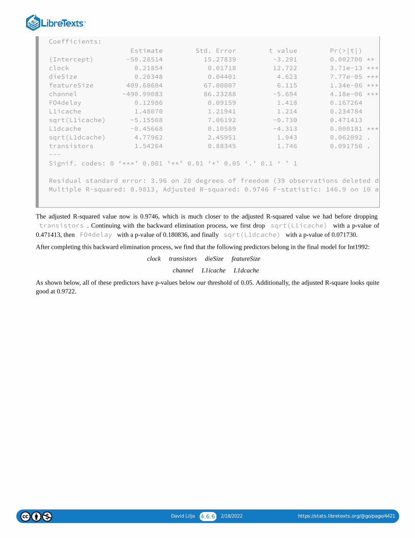
David Lilja 4.6.6 2/18/2022 https://stats.libretexts.org/@go/page/4421

The adjusted R-squared value now is 0.9746, which is much closer to the adjusted R-squared value we had before dropping transistors . Continuing with the backward elimination process, we first drop sqrt(L1icache) with a p-value of

0.471413, then FO4delay with a p-value of 0.180836, and finally sqrt(L1dcache) with a p-value of 0.071730.

After completing this backward elimination process, we find that the following predictors belong in the final model for Int1992:

clock transistors dieSize featureSize

channel L1icache L1dcache

As shown below, all of these predictors have p-values below our threshold of 0.05. Additionally, the adjusted R-square looks quitegood at 0.9722.

Coefficients:

Estimate Std. Error t value Pr(>|t|)

(Intercept) -50.28514 15.27839 -3.291 0.002700 **

clock 0.21854 0.01718 12.722 3.71e-13 ***

dieSize 0.20348 0.04401 4.623 7.77e-05 ***

featureSize 409.68604 67.00007 6.115 1.34e-06 ***

channel -490.99083 86.23288 -5.694 4.18e-06 ***

FO4delay 0.12986 0.09159 1.418 0.167264

L1icache 1.48070 1.21941 1.214 0.234784

sqrt(L1icache) -5.15568 7.06192 -0.730 0.471413

L1dcache -0.45668 0.10589 -4.313 0.000181 ***

sqrt(L1dcache) 4.77962 2.45951 1.943 0.062092 .

transistors 1.54264 0.88345 1.746 0.091750 .

---

Signif. codes: 0 ‘***’ 0.001 ‘**’ 0.01 ‘*’ 0.05 ‘.’ 0.1 ‘ ’ 1

Residual standard error: 3.96 on 28 degrees of freedom (39 observations deleted d

Multiple R-squared: 0.9813, Adjusted R-squared: 0.9746 F-statistic: 146.9 on 10 a

David Lilja 4.6.7 2/18/2022 https://stats.libretexts.org/@go/page/4421

This example illustrates that you cannot always look at only the p-values to determine which potential predictors to eliminate ineach step of the backward elimination process. You also must be careful to look at the broader picture, such as changes in theadjusted R-squared value and large changes in the p-values of other predictors, after each change to the model.

> int92.lm <update(int92.lm, .~. -sqrt(L1dcache))

> summary(int92.lm)

Call:

lm(formula = nperf ~ clock + dieSize + featureSize + channel +

L1icache + L1dcache + transistors, data = int92.dat)

Residuals:

Min 1Q Median 3Q Max

-10.1742 -1.5180 0.1324 1.9967 10.1737

Coefficients:

Estimate Std. Error t value Pr(>|t|)

(Intercept) -34.17260 5.47413 -6.243 6.16e-07 ***

clock 0.18973 0.01265 15.004 9.21e-16 ***

dieSize 0.11751 0.02034 5.778 2.31e-06 ***

featureSize 305.79593 52.76134 5.796 2.20e-06 ***

channel -328.13544 53.04160 -6.186 7.23e-07 ***

L1icache 0.78911 0.16045 4.918 2.72e-05 ***

L1dcache -0.23335 0.03222 -7.242 3.80e-08 ***

transistors 3.13795 0.51450 6.099 9.26e-07 ***

---

Signif. codes: 0 ‘***’ 0.001 ‘**’ 0.01 ‘*’ 0.05 ‘.’ 0.1 ‘ ’ 1

Residual standard error: 4.141 on 31 degrees of freedom (39 observations deleted

Multiple R-squared: 0.9773, Adjusted R-squared: 0.9722 F-statistic: 191 on 7 and

1 2/18/2022

CHAPTER OVERVIEW5: PREDICTING RESPONSES

PREDICTION is typically the primary goal of most regression modeling projects. That is, the model developer wants to use the model toestimate or predict the system’s response if it were operated with input values that were never actually available in any of the measuredsystems. For instance, we might want to use the model we developed using the Int2000 data set to predict the performance of a newprocessor with a clock frequency, a cache size, or some other parameter combination that does not exist in the data set. By inserting this newcombination of parameter values into the model, we can compute the new processor’s expected performance when executing that benchmarkprogram.

Because the model was developed using measured data, the coefficient values necessarily are only estimates. Consequently, any predictionswe make with the model are also only estimates. The summary() function produces useful statistics about the regression model’s quality,such as the R2 and adjusted R2 values. These statistics offer insights into how well the model explains variation in the data. The bestindicator of any regression model’s quality, however, is how well it predicts output values. The R environment provides some powerfulfunctions that help us predict new values from a given model and evaluate the quality of these predictions.

5.1: DATA SPLITTING FOR TRAINING AND TESTING5.2: TRAINING AND TESTING5.3: PREDICTING ACROSS DATA SETS5.4: SECTION 5-5.5: SECTION 6-

David Lilja 5.1.1 1/28/2022 https://stats.libretexts.org/@go/page/4423

5.1: Data Splitting for Training and TestingIn Chapter 4 we used all of the data available in the int00.dat data frame to select the appropriate predictors toinclude in the final regression model. Because we computed the model to fit this particular data set, we cannot now use thissame data set to test the model’s predictive capabilities. That would be like copying exam answers from the answer keyand then using that same answer key to grade your exam. Of course you would get a perfect result. Instead, we must useone set of data to train the model and another set of data to test it.

The difficulty with this train-test process is that we need separate but similar data sets. A standard way to find these twodifferent data sets is to split the available data into two parts. We take a random portion of all the available data and call itour training set. We then use this portion of the data in the lm() function to compute the specific values of the model’scoefficients. We use the remaining portion of the data as our testing set to see how well the model predicts the results,compared to this test data.

The following sequence of operations splits the int00.dat data set into the training and testing sets:

rows <nrow(int00.dat)

f <0.5

upper_bound <floor(f * rows)

permuted_int00.dat <int00.dat[sample(rows), ]

train.dat <permuted_int00.dat[1:upper_bound, ]

test.dat <permuted_int00.dat[(upper_bound+1):rows, ]

The first line assigns the total number of rows in the int00.dat data frame to the variable rows . The next lineassigns to the variable f  the fraction of the entire data set we wish to use for the training set. In this case, we somewhatarbitrarily decide to use half of the data as the training set and the other half as the testing set. The floor() functionrounds its argument value down to the nearest integer. So the line upper_bound <floor(f * rows) assignsthe middle row’s index number to the variable upper_bound .

The interesting action happens in the next line. The sample() function returns a permutation of the integers between1 and n when we give it the integer value n as its input argument. In this code, the expression sample(rows) returnsa vector that is a permutation of the integers between 1 and rows , where rows is the total number of rows in the int00.dat data frame. Using this vector as the row index for this data frame gives a random permutation of all of the

rows in the data frame, which we assign to the new data frame, permuted_int00.dat. The next two lines assignthe lower portion of this new data frame to the training data set and the top portion to the testing data set, respectively. Thisrandomization process ensures that we obtain a new random selection of the rows in the train-and-test data sets every timewe execute this sequence of operations.

David Lilja 5.2.1 2/18/2022 https://stats.libretexts.org/@go/page/4424

5.2: Training and TestingWith the data set partitioned into two randomly selected portions, we can train the model on the first portion, and test it on thesecond portion. Figure 5.1shows the overall flow of this training and testing process. We next explain the details of this process totrain and test the model we previously developed for the Int2000 benchmark results.

Figure 5.1: The training and testing process for evaluating the predictions produced by a regression model.

The following statement calls the lm() function to generate a regression model using the predictors we identified inChapter 4 and the train.dat  data frame we extracted in the previous section. It then assigns this model to the variable int00_new.lm. We refer to this process of computing the model’s coefficients as training the regression model.

The predict() function takes this new model as one of its arguments. It uses this model to compute the predicted outputswhen we use the test.dat data frame as the input, as follows:

predicted.dat <predict(int00_new.lm, newdata=test.dat)

We define the difference between the predicted and measured performance for each processor i to be ∆ = Predictedi − Measured ,where Predicted is the value predicted by the model, which is stored in the data frame predicted.dat , and Measured is theactual measured performance response, which we previously assigned to the test.dat  data frame. The following statementcomputes the entire vector of these ∆ values and assigns the vector to the variable delta .

delta <predicted.dat test.dat$nperf

Note that we use the $ notation to select the column with the output value, nperf , from the test.dat data frame.

The mean of these ∆ differences for n different processors is:

A confidence interval computed for this mean will give us some indication of how well a model trained on the train.dat

data set predicted the performance of the processors in the test.dat data set. The  t.test() function computes aconfidence interval for the desired confidence level of these ∆ values as follows:

int00_new.lm <lm(nperf ~ clock + cores + voltage + channel + L1icache +

sqrt(L1icache) + L1dcache + sqrt(L1dcache) + L2cache + sqrt(L2cache), data = trai

i i

i i

i

=Δ̄1

n∑n

i=1Δi

i

David Lilja 5.2.2 2/18/2022 https://stats.libretexts.org/@go/page/4424

> t.test(delta, conf.level = 0.95)

One Sample t-test

data: delta

t = -0.65496, df = 41, p-value = 0.5161

alternative hypothesis: true mean is not equal to 0

95 percent confidence interval:-2.232621 1.139121

sample estimates: mean of x -0.5467502

If the prediction were perfect, then ∆ = 0. If ∆ > 0, then the model predicted that the performance would be greater than it actuallywas. A ∆ < 0, on the other hand, means that the model predicted that the performance was lower than it actually was.Consequently, if the predictions were reasonably good, we would expect to see a tight confidence interval around zero. In this case,we obtain a 95 percent confidence interval of [-2.23, 1.14]. Given that nperf is scaled to between 0 and 100, this is a reasonablytight confidence interval that includes zero. Thus, we conclude that the model is reasonably good at predicting values in the test.dat  data set when trained on the train.dat data set.

Another way to get a sense of the predictions’ quality is to generate a scatter plot of the ∆ values using the plot() function:

plot(delta)

This function call produces the plot shown in Figure 5.2. Good predictions would produce a tight band of values uniformlyscattered around zero. In this figure, we do see such a distribution, although there are a few outliers that are more than ten pointsabove or below zero.

It is important to realize that the sample() function will return a different random permutation each time we execute it. Thesediffering permutations will partition different processors (i.e., rows in the data frame) into the train and test sets. Thus, if we runthis experiment again with exactly the same inputs, we will likely get a different confidence interval and ∆ scatter plot. Forexample, when we repeat the same test five times with identical inputs, we obtain the following confidence intervals: [-1.94, 1.46],[-1.95, 2.68], [-2.66, 3.81], [-6.13, 0.75], [-4.21, 5.29]. Similarly, varying the fraction of the data we assign to the train and test setsby changing f = 0.5 also changes the results.

It is good practice to run this type of experiment several times and observe how the results change. If you see the results varywildly when you re-run these tests, you have good reason for concern. On the other hand, a series of similar results does notnecessarily mean your results are good, only that they are consistently reproducible. It is often easier to spot a bad model than todetermine that a model is good.

Based on the repeated confidence interval results and the corresponding scatter plot, similar to Figure 5.2, we conclude that thismodel is reasonably good at predicting the performance of a set of processors when the model is trained on a different set ofprocessors executing the same benchmark program. It is not perfect, but it is also not too bad. Whether the differences are largeenough to warrant concern is up to you.

i i

i

i

i

David Lilja 5.2.3 2/18/2022 https://stats.libretexts.org/@go/page/4424

Figure 5.2: An example scatter plot of the differences between the predicted and actual performance results for the Int2000benchmark when using the data-splitting technique to train and test the model.

David Lilja 5.3.1 12/10/2021 https://stats.libretexts.org/@go/page/4425

5.3: Predicting Across Data SetsAs we saw in the previous section, data splitting is a useful technique for testing a regression model. If you have other datasets, you can use them to further test your new model’s capabilities.

In our situation, we have several additional benchmark results in the data file that we can use for these tests. As anexample, we use the model we developed from the Int2000 data to predict the Fp2000 benchmark’s performance.

We first train the model developed using the Int2000 data, int00.lm , using all the Int2000 data available in the int00.dat data frame. We then predict the Fp2000 results using this model and the fp00.dat data. Again, we

assign the differences between the predicted and actual results to the vector delta . Figure 5.3 shows the overall dataflow for this training and testing. The corresponding R commands are:

Figure 5.3: Predicting the Fp2000 results using the model developed with the Int2000 data.

The resulting confidence interval for the delta values contains zero and is relatively small. This result suggests thatthe model developed using the Int2000 data is reasonably good at predicting the Fp2000 benchmark program’s results. Thescatter plot in Figure 5.4 shows the resulting delta values for each of the processors we used in the prediction. Theresults tend to be randomly distributed around zero, as we would expect from a good regression model. Note, however,that some of the values differ significantly from zero. The maximum positive deviation is almost 20, and the magnitude of

> int00.lm <lm(nperf ~ clock + cores + voltage + channel +

L1icache + sqrt(L1icache) + L1dcache + sqrt(L1dcache) + L2cache +

sqrt(L2cache), data = int00.dat)> predicted.dat <predict(int00.lm, newdata=f

> delta <predicted.dat fp00.dat$nperf

> t.test(delta, conf.level = 0.95)

One Sample t-test

data: delta

t = 1.5231, df = 80, p-value = 0.1317

alternative hypothesis: true mean is not equal to 0

95 percent confidence interval:

-0.4532477 3.4099288 sample estimates:

mean of x

1.478341

David Lilja 5.3.2 12/10/2021 https://stats.libretexts.org/@go/page/4425

the largest negative value is greater than 43. The confidence interval suggests relatively good results, but this scatter plotshows that not all the values are well predicted.

Figure 5.4: A scatter plot of the differences between the predicted and actual performance results for the Fp2000benchmark when predicted using the Int2000 regression model.

As a final example, we use the Int2000 regression model to predict the results of the benchmark program’s future Int2006version. The R code to compute this prediction is:

In this case, the confidence interval for the delta values does not include zero. In fact, the mean value of thedifferences is 50.9096, which indicates that the average of the model-predicted values is substantially larger than the actualaverage value. The scatter plot shown in Figure 5.5 further confirms that the predicted values are all much larger than theactual values.

This example is a good reminder that models have their limits. Apparently, there are more factors that affect theperformance of the next generation of the benchmark programs, Int2006, than the model we developed using the Int2000results captures. To develop a model that better predicts future performance, we would have to uncover those factors.Doing so requires a deeper understanding of the factors that affect computer performance, which is beyond the scope ofthis tutorial.

> int00.lm <lm(nperf ~ clock + cores + voltage + channel + L1icache + sqrt(L

sqrt(L1dcache) + L2cache + sqrt(L2cache), data = int00.dat)> predicted.dat <

> delta <predicted.dat int06.dat$nperf

> t.test(delta, conf.level = 0.95)

One Sample t-test

data: delta

t = 49.339, df = 168, p-value < 2.2e-16

alternative hypothesis: true mean is not equal to 0

95 percent confidence interval: 48.87259 52.94662

sample estimates:

mean of x

50.9096

David Lilja 5.3.3 12/10/2021 https://stats.libretexts.org/@go/page/4425

Figure 5.5: A scatter plot of the differences between the predicted and actual performance results for the Int2006benchmark, predicted using the Int2000 regression model.

David Lilja 1 1/7/2022 https://stats.libretexts.org/@go/page/4427

Welcome to the Statistics Library. This Living Library is a principal hub of the LibreTexts project, which is a multi-institutional collaborative venture to develop the next generation of open-access texts to improve postsecondary educationat all levels of higher learning. The LibreTexts approach is highly collaborative where an Open Access textbookenvironment is under constant revision by students, faculty, and outside experts to supplant conventional paper-basedbooks.

Campus Bookshelves Bookshelves

Learning Objects

David Lilja 5.5.1 1/14/2022 https://stats.libretexts.org/@go/page/4428

Edit page

Drag and drop

Classifications

Working with templates

5.5: Section 6-

Your page has been created!Remove this content and add your own.

Click the Edit page button in your user bar. You will see a suggested structure for your content. Add your content andhit Save.

Tips:

Drag one or more image files from your computer and drop them onto your browser window to add them to yourpage.

Tags are used to link pages to one another along common themes. Tags are also used as markers for the dynamicorganization of content in the CXone Expert framework.

CXone Expert templates help guide and organize your documentation, making it flow easier and more uniformly.Edit existing templates or create your own.

Visit for all help topics.

David Lilja 6.1 12/10/2021 https://stats.libretexts.org/@go/page/4436

6: Reading Data into the R EnvironmentAS we have seen, the R environment provides some powerful functions to quickly and relatively easily develop and testregression models. Ironically, simply reading the data into R in a useful format can be one of the most difficult aspects ofdeveloping a model. R does not lack good input-output capabilities, but data often comes to the model developer in amessy form. For instance, the data format may be inconsistent, with missing fields and incorrectly recorded values. Gettingthe data into the format necessary for analysis and modeling is often called data cleaning. The specific steps necessary to“clean” data are heavily dependent on the data set and are thus beyond the scope of this tutorial. Suffice it to say that youshould carefully examine your data before you use it to develop any sort of regression model. Section 2.2 provides a fewthoughts on data cleaning.

In Chapter 2, we provided the functions used to read the example data into the R environment, but with no explanationabout how they worked. In this chapter, we will look at these functions in detail, as specific examples of how to read a dataset into R. Of course, the details of the functions you may need to write to input your data will necessarily change to matchthe specifics of your data set.

6.1: Reading CSV files

David Lilja 6.1.1 2/18/2022 https://stats.libretexts.org/@go/page/4430

6.1: Reading CSV filesPerhaps the simplest format for exchanging data among computer systems is the de facto standard comma separated values, or csv,file. R provides a function to directly read data from a csv file and assign it to a data frame:

> processors <- read.csv("all-data.csv")

The name between the quotes is the name of the csv-formatted file to be read. Each file line corresponds to one data record.Commas separate the individual data fields in each record. This function assigns each data record to a new row in the data frame,and assigns each data field to the corre- sponding column. When this function completes, the variable processors containsall the data from the file  all-data.csv nicely organized into rows and columns in a data frame.

If you type processors to see what is stored in the data frame, you will get a long, confusing list of data. Typing

> head(processors)

will show a list of column headings and the values of the first few rows of data. From this list, we can determine which columns toextract for our model development. Although this is conceptually a simple problem, the execution can be rather messy, dependingon how the data was collected and organized in the file.

As with any programming language, R lets you define your own func- tions. This feature is useful when you must perform asequence of opera- tions multiple times on different data pieces, for instance. The format for defining a function is:

function-name <- function(a1, a2, ...) { R expressions

return(object)

}

where function-name is the function name you choose and a1, a2, ... is the list of arguments in your function.The R system evaluates the expres- sions in the body of the definition when the function is called. A function can return any type ofdata object using the return() statement.

We will define a new function called extract_data to extract all the rows that have a result for the given benchmarkprogram from the processors  data frame. For instance, calling the function as follows:

> int92.dat <- extract_data("Int1992")

> fp92.dat <- extract_data("Fp1992")

> int95.dat <- extract_data("Int1995")

> fp95.dat <- extract_data("Fp1995")

> int00.dat <- extract_data("Int2000")

> fp00.dat <- extract_data("Fp2000")

> int06.dat <- extract_data("Int2006")

> fp06.dat <- extract_data("Fp2006")

extracts every row that has a result for the given benchmark program and assigns it to the corresponding data frame, int92.dat, fp92.dat , and so on.

We define the extract_data function as follows:

David Lilja 6.1.2 2/18/2022 https://stats.libretexts.org/@go/page/4430

The first line with the paste functions looks rather complicated. How- ever, it simply forms the name of the column with thegiven benchmark results. For example, when extract_data is called with Int2000 as the ar- gument, the nested paste functions simply concatenate the strings " Spec ", " Int2000 ", and " ..average.base. ". The final string

corresponds to the name of the column in the processors data frame that contains the perfor- mance results for the Int2000 benchmark, " SpecInt2000..average.base. ".

The next line calls the function get_column , which selects all the rows with the desired column name. In this case, thatcolumn contains the actual performance result reported for the given benchmark program, perf . The next four lines computethe normalized performance value, nperf , from the perf value we obtained from the data frame. The following sequenceof calls to get_column extracts the data for each of the predictors we intend to use in developing the regression model. Notethat the second parameter in each case, such as " Processor.Clock..MHz. ", is the name of a column in the processors data frame. Finally, the data.frame() function is a predefined R function that assembles all its arguments

into a single data frame. The new function we have just defined, extract_data() , returns this new data frame.

Next, we define the get_column() function to return all the data in a given column for which the given benchmark programhas been defined:

get_column <- function(x,y) {

benchmark <- paste(paste("Spec",x,sep=""), "..average.base.", sep="")

ix <- !is.na(processors[,benchmark]) return(processors[ix,y])

}

extract_data <- function(benchmark) {

temp <- paste(paste("Spec",benchmark,sep=""), "..average.base.", sep="")

perf <- get_column(benchmark,temp)

max_perf <- max(perf)

min_perf <- min(perf)

range <- max_perf - min_perf

nperf <- 100 * (perf - min_perf) / range

clock <- get_column(benchmark,"Processor.Clock..MHz.")

threads <- get_column(benchmark,"Threads.core")

cores <- get_column(benchmark,"Cores")

TDP <- get_column(benchmark,"TDP")

transistors <- get_column(benchmark,"Transistors..millions.")

dieSize <- get_column(benchmark,"Die.size..mm.2.")

voltage <- get_column(benchmark,"Voltage..low.")

featureSize <- get_column(benchmark,"Feature.Size..microns.")

channel <- get_column(benchmark,"Channel.length..microns.")

FO4delay <- get_column(benchmark,"FO4.Delay..ps.")

L1icache <- get_column(benchmark,"L1..instruction...on.chip.")

L1dcache <- get_column(benchmark,"L1..data...on.chip.")

L2cache <- get_column(benchmark,"L2..on.chip.")

L3cache <- get_column(benchmark,"L3..on.chip.")

return(data.frame(nperf, perf, clock, threads, cores, TDP, transistors, dieSize,

voltage, featureSize, channel, FO4delay, L1icache, L1dcache, L2cache, L3cache))

}

David Lilja 6.1.3 2/18/2022 https://stats.libretexts.org/@go/page/4430

The argument x is a string with the name of the benchmark program, and y is a string with the name of the desired column.The nested paste() func- tions produce the same result as the extract_data() function. The is.na() functionperforms the interesting work. This function returns a vector with “ 1 ” values corresponding to the row numbers in the processors data frame that have NA values in the column selected by the benchmark index. If there is a value in that

location, is.na() will return a corresponding value that is a 0 . Thus, is.na indicates which rows are missingperformance results for the benchmark of interest. Inserting the exclamation point in front of this function complements its output.As a result, the variable ix will con- tain a vector that identifies every row that contains performance results for the indicatedbenchmark program. The function then extracts the selected rows from the processors data frame and returns them.

These types of data extraction functions can be somewhat tricky to write, because they depend so much on the specific format ofyour input file. The functions presented in this chapter are a guide to writing your own data extraction functions.

David Lilja 7.1 2/11/2022 https://stats.libretexts.org/@go/page/4443

7: SummaryLINEAR regression modeling is one of the most basic of a broad collection of data mining techniques. It can demonstratethe relationships between the inputs to a system and the corresponding output. It also can be used to predict the outputgiven a new set of input values. While the specifics for developing a regression model will depend on the details of yourdata, there are several key steps to keep in mind when developing a new model using the R programming environment:

1. Read your data into the R environment.

As simple as it sounds, one of the trickiest tasks oftentimes is simply reading your data into R. Because you may nothave controlled how data was collected, or in what format, be prepared to spend some time writing new functions toparse your data and load it into an R data frame. Chapter 6 provides an example of reading a moderately complicatedcsv file into R.

2. Sanity check your data.

Once you have your data in the R environment, perform some sanity checks to make sure that there is nothingobviously wrong with the data. The types of checks you should perform depend on the specifics of your data. Somepossibilities include:

Finding the values’ minimum, maximum, average, and standard deviation in each data frame column.

Looking for any parameter values that seem suspiciously outside the expected limits.

Determining the fraction of missing ( NA ) values in each column to ensure that there is sufficient data available.

Determining the frequency of categorical parameters, to see if any unexpected values pop up.

Any other data-specific tests.

Ultimately, you need to feel confident that your data set’s values are reasonable and consistent.

3. Visualize your data.

It is always good to plot your data, to get a basic sense of its shape and ensure that nothing looks out of place. Forinstance, you may expect to see a somewhat linear relationship between two parameters. If you see something else,such as a horizontal line, you should investigate further. Your assumption about a linear relationship could be wrong, orthe data may be corrupted (see item no. 2 above). Or perhaps something completely unexpected is going on.Regardless, you must understand what might be happening before you begin developing the model. The pairs() function is quite useful for performing this quick visual check, as described in Section 4.1.

4. Identify the potential predictors.

Before you can begin the backward elimination process, you must identify the set of all possible predictors that couldgo into your model. In the simplest case, this set consists of all of the available columns in your data frame. However,you may know that some of the columns will not be useful, even before you begin constructing the model. Forexample, a column containing only a few valid entries probably is not useful in a model. Your knowledge of the systemmay also give you good reason to eliminate a parameter as a possible predictor, much as we eliminated TDP as apossible predictor in Section 4.2, or to include some of the parameters’ non-linear functions as possible predictors, aswe did when we added the square root of the cache size terms to our set of possible predictors.

5. Select the predictors.

Once you have identified the potential predictors, use the backward elimination process described in Section 4.3 toselect the predictors you’ll include in the final model, based on the significance threshold you decide to use.

6. Validate the model.

Examine your model’s R value and the adjusted-R value. Use residual analysis to further examine the model’squality. You also should split your data into training and testing sets, and then see how well your model predicts valuesfrom the test set.

7. Predict.

2 2

David Lilja 7.2 2/11/2022 https://stats.libretexts.org/@go/page/4443

Now that you have a model that you feel appropriately explains your data, you can use it to predict previously unknownoutput values.

A deep body of literature is devoted to both statistical modeling and the R language. If you want to learn more about R as aprogramming language, many good books are available, including [11, 12, 15, 16]. These books focus on specificstatistical ideas and use R as the computational language [1, 3, 4, 14]. Finally, this book [9] gives an introduction tocomputer performance measurement.

As you continue to develop your data-mining skills, remember that what you have developed is only a model. Ideally, it isa useful tool for explaining the variations in your measured data and understanding the relationships between inputs andoutput. But like all models, it is only an approximation of the real underlying system, and is limited in what it can tell usabout that system. Proceed with caution.

David Lilja 8.1 2/4/2022 https://stats.libretexts.org/@go/page/4450

8: A Few Things to Try NextHERE are a few suggested exercises to help you learn more about regression modeling using R.

1. Show how you would clean the data set for one of the selected benchmark results (Int1992, Int1995, etc.). For example,for every column in the data frame, you could:

Compute the average, variance, minimum, and maximum.

Sort the column data to look for outliers or unusual patterns.

Determine the fraction of NA values for each column.

How else could you verify that the data looks reasonable?

2. Plot the processor performance versus the clock frequency for each of the benchmark results, similar to Figure 3.1.

3. Develop a one-factor linear regression model for all the benchmark results. What input factor should you use as thepredictor?

4. Superimpose your one-factor models on the corresponding scatter plots of the data (see Figure 3.2).

5. Evaluate the quality of the one-factor models by discussing the residuals, the p-values of the coefficients, the residualstandard errors, the R values, the F-statistic, and by performing appropriate residual analysis.

6. Generate a pair-wise comparison plot for each of the benchmark results, similar to Figure 4.1.

7. Develop a multi-factor linear regression model for each of the benchmark results. Which predictors are the same andwhich are different across these models? What other similarities and differences do you see across these models?

8. Evaluate the multi-factor models’ quality by discussing the residuals, the p-values of the coefficients, the residualstandard errors, the R values, the F-statistic, and by performing appropriate residual analysis.

9. Use the regression models you’ve developed to complete the follow- ing tables, showing how well the models fromeach row predict the benchmark results in each column. Specifically, fill in the x and y values so that x is the mean ofthe delta values for the predictions and y is the width of the corresponding 95 percent confidence in- terval. Youneed only predict forwards in time. For example, it is reasonable to use the model developed with Int1992 data topredict Int2006 results, but it does not make sense to use a model developed with Int2006 data to predict Int1992results.

Int1992 Int1995 Int2000 Int2006

Int1992Int1995Int2000Int2006Fp1992Fp1995Fp2000Fp2006

x(±y)

x(±y)

x(±y)x(±y)

x(±y)x(±y)

x(±y)x(±y)x(±y)

x(±y)x(±y)x(±y)

x(±y)x(±y)x(±y)x(±y)x(±y)x(±y)x(±y)x(±y)

Fp1992 Fp1995 Fp2000 Fp2006

Int1992Int1995Int2000Int2006Fp1992Fp1995Fp2000

x(±y)

x(±y)

x(±y)x(±y)

x(±y)x(±y)

x(±y)x(±y)x(±y)

x(±y)x(±y)x(±y)

x(±y)x(±y)x(±y)x(±y)x(±y)x(±y)x(±y)

2

2

David Lilja 8.2 2/4/2022 https://stats.libretexts.org/@go/page/4450

Fp2006 x(±y)

10. What can you say about these models’ predictive abilities, based on the results from the previous problem? Forexample, how well does a model developed for the integer benchmarks predict the same-year performance of thefloating-point benchmarks? What about predic- tions across benchmark generations?

11. In the discussion of data splitting, we defined the value f as the fraction of the complete data set used in the training set.For the Fp2000 data set, plot a 95 percent confidence interval for the mean of delta for f = [0.1, 0.2, ..., 0.9]. Whatvalue of f gives the best result (i.e., the smallest confidence interval)? Repeat this test n = 5 times to see how the bestvalue of f changes.

12. Repeat the previous problem, varying f for all the other data sets.

IndexDData Frames (R)

2.4: Data Frames

Glossary

Sample Word 1 | Sample Definition 1