Ultrasonic Evaluation of Microstructure in Pipe Steels
179
Ultrasonic Evaluation of Microstructure in Pipe Steels by Jacob Kennedy A thesis submitted in partial fulfillment of the requirements for the degree of Master of Science in Materials Engineering Department of Chemical and Materials Engineering University of Alberta © Jacob Kennedy, 2015
Transcript of Ultrasonic Evaluation of Microstructure in Pipe Steels

Ultrasonic Evaluation of Microstructure in Pipe Steels
by
Jacob Kennedy
A thesis submitted in partial fulfillment of the requirements for the degree of
Master of Science
in
Materials Engineering
Department of Chemical and Materials Engineering
University of Alberta
© Jacob Kennedy, 2015

ii
Abstract
Traditionally in pipeline steels and welds, ultrasonic testing (UT) has been used for crack and/or
flaw detection. The work presented in this Thesis explores the use of this technique to characterize
the microstructure of pipe steels. Ultrasonic velocity calculations, for shear and longitudinal
waves, done with the stiffness tensor of a 1050 steel showed that shear velocity exhibits a greater
difference between structures such as ferrite, mixed ferrite-pearlite, and martensite, than
longitudinal velocity. Experiments were carried out, through thickness skelp investigation of L80
and X70 steels, annealing of interstitial free steel and structure variation in L80, 4130 and 5160.
The ultrasonic velocity and attenuation of shear and longitudinal waves were measured through
the thickness of L80 and X70 pipe skelps and did not vary significantly. XRD was performed
through the thickness as well. Interstitial free steel was ultrasonically tested at room temperature
after different annealing times. Both shear and longitudinal ultrasonic velocity changed as
recrystallization progressed, while attenuation changed during grain growth. Structure variations
after heat treatment in L80, 4130 and 5160 all showed a decrease in ultrasonic shear wave velocity
in martensite when compared with mixed structure of ferrite and pearlite, confirming the velocity
calculation results. The longitudinal velocity did not vary with structure. The attenuation of both
shear and longitudinal waves also decreased in martensite compared with mixed ferrite-pearlite.
Both shear and longitudinal ultrasonic waves had properties which varied with different structural
properties and had the potential to be useful tools in microstructural characterization. The
ultrasonic shear velocity showed a decrease from ferrite-pearlite (3268 m/s) to martensite (3207
m/s) as did the longitudinal attenuation (0.25 dB/mm for ferrite-pearlite and 0.17 dB/mm for
martensite)

iii
Acknowledgements
I would like to thank my supervisors Professor Hani Henein and Professor Douglas Ivey for their
support and guidance. I would also like to thank Dr. Barry Wiskel for his input and counsel through
the entirety of this work. Thanks to the post-doctoral fellows and students in the Advanced
Materials and Processing Laboratory (AMPL), as well as Advaita Bhatnagar for her assistance
with the metallography done for the L80. I could not have done this without all of you.
Special thanks also to Evraz Inc. NA, Trans-Canada Pipelines, Enbridge, Alliance Pipelines and
UT Quality for their sponsorship of this work along with the Natural Sciences and Engineering
Research Council (NSERC) of Canada.
Thanks to my family and friends for their help. I would also like to thank Jaime, a better partner
could not have been found to support and encourage me through this work.

iv
Table of Contents
Abstract .......................................................................................................................................... ii
Acknowledgements ...................................................................................................................... iii
Table of Contents ......................................................................................................................... iv
List of Tables .............................................................................................................................. viii
List of Figures ............................................................................................................................... ix
List of Symbols and Acronyms ................................................................................................. xiii
Introduction ................................................................................................................................... 1
Chapter 1 Literature Review ....................................................................................................... 2
1.1 General Concepts in Steel Microstructure ............................................................................ 2
1.1.1 Phase and Structure ........................................................................................................ 2
1.1.2 Crystallographic Texture ............................................................................................... 7
1.2 General Concepts in Ultrasonic Testing................................................................................ 8
1.2.1 Wave Types ................................................................................................................... 8
1.2.2 Interfaces ...................................................................................................................... 10
1.2.3 Flaw Detection ............................................................................................................. 12
1.3 Ultrasonic Velocity and Attenuation ................................................................................... 13
1.3.1 Ultrasonic Velocity ...................................................................................................... 13
1.3.2 Ultrasonic Attenuation ................................................................................................. 13
1.4 Ultrasonic Velocity and Microstructure .............................................................................. 14
1.4.1 Ultrasonic Velocity and Morphology .......................................................................... 14
1.4.2 Ultrasonic Velocity and Precipitates ............................................................................ 15
1.4.3 Ultrasonic Velocity and Orientation ............................................................................ 16
1.4.4 Ultrasonic Velocity and Grain Size ............................................................................. 18
1.4.5 Ultrasonic Velocity and Stress ..................................................................................... 18
1.4.6 Ultrasonic Velocity Summary...................................................................................... 19
1.5 Ultrasonic Attenuation and Microstructure ......................................................................... 19
1.5.1 Ultrasonic Attenuation and Morphology ..................................................................... 19
1.5.2 Ultrasonic Attenuation and Precipitation ..................................................................... 20
1.5.3 Ultrasonic Attenuation and Orientation ....................................................................... 20
1.5.4 Ultrasonic Attenuation and Grain Size ........................................................................ 21
1.5.5 Ultrasonic Attenuation and Dislocation Density ......................................................... 23

v
1.5.6 Ultrasonic Attenuation Summary ................................................................................ 23
1.6 Summary ............................................................................................................................. 24
Chapter 2 Velocity Calculations ................................................................................................ 25
2.1 Anisotropic Velocity Formulation ...................................................................................... 25
2.2 Anisotropic Velocity Results .............................................................................................. 28
2.2.1 Anisotropic Polycrystal ................................................................................................ 29
2.3 Young’s Modulus Velocity Calculations ............................................................................ 32
2.4 Isotropic Velocity Calculation Formulations ...................................................................... 33
2.5 Isotropic Assumption Velocity Simulations ....................................................................... 36
2.6 Summary ............................................................................................................................. 40
Chapter 3 Experimental Methods and Results ........................................................................ 41
3.1 Steels Studied ..................................................................................................................... 41
3.2 Ultrasonic Testing Methodology ...................................................................................... 42
3.2.1 Ultrasonic Equipment .................................................................................................. 42
3.2.2 Pressure and Thickness Effects .................................................................................... 42
3.2.3 Experimental Setup ...................................................................................................... 45
3.2.4 Velocity Measurements ............................................................................................... 47
3.2.5 Attenuation Measurements .......................................................................................... 49
3.2.6 Ultrasonic Measurement Uncertainty .......................................................................... 51
3.3 Pipe Skelp Through Thickness Investigation ................................................................. 52
3.3.1 Experimental Design .................................................................................................... 53
3.3.2 XRD Analysis .............................................................................................................. 54
3.3.3 Ultrasonic Tests ........................................................................................................... 56
3.4 Interstitial Free Steel Annealing ...................................................................................... 57
3.4.1 Experimental Design .................................................................................................... 57
3.4.2 Metallography .............................................................................................................. 58
3.4.3 Ultrasonic Tests ........................................................................................................... 59
3.5 L80 Steel Microstructure Variation ................................................................................ 59
3.5.1 Experimental Design .................................................................................................... 60
3.5.2 Ultrasonic Tests ........................................................................................................... 61
3.5.3 Vickers Hardness ......................................................................................................... 63
3.5.4 Metallography .............................................................................................................. 64

vi
3.5.5 Tensile Tests ................................................................................................................ 66
3.6 Industrial UT ..................................................................................................................... 71
3.6.1 5160 and 4130 Experimental Design ........................................................................... 71
3.6.2 5160 and 4130 Ultrasonic Tests ................................................................................... 72
3.7 Summary of Experimental Methods and Results ................................................................ 74
Chapter 4 Discussion .................................................................................................................. 75
4.1 Pipe Skelp Through Thickness Investigation ...................................................................... 75
4.1.1 Ultrasonic Velocity Through Skelp Thickness ............................................................ 75
4.1.2 Through Thickness Attenuation ................................................................................... 82
4.1.3 Pipe Skelp Through Thickness Summary .................................................................... 84
4.2 Annealing Interstitial Free Steel .......................................................................................... 84
4.2.1 Effect of Holding Time on Microstructure .................................................................. 84
4.2.2 Effect on Ultrasonic Velocity ...................................................................................... 89
4.2.3 Effect on Ultrasonic Attenuation ................................................................................. 94
4.2.4 Annealing IF Steel Summary ....................................................................................... 97
4.3 L80 Steel Microstructure Variation..................................................................................... 98
4.3.1 Heat Treated L80 Small Bars ....................................................................................... 98
4.3.2 Heat Treated L80 Long Bars ...................................................................................... 104
4.3.3 L80 Tensile Tests and Ultrasonic Properties ............................................................. 112
4.3.4 L80 Microstructure Variation Summary .................................................................... 124
4.4 Industrial UT ..................................................................................................................... 125
4.4.1 4130 Heat Treated Samples ....................................................................................... 125
4.4.2 5160 Heat Treated Samples ....................................................................................... 129
4.4.3 Industrial UT Summary ............................................................................................. 132
4.5 Velocity Comparison Across All Samples ........................................................................ 133
Chapter 5 Conclusions, Recommendations and Future Work ............................................. 135
5.1 Conclusions ....................................................................................................................... 135
5.2 Industrial Implications....................................................................................................... 136
5.3 Recommendations and Future Work ................................................................................. 137
References .................................................................................................................................. 138
Appendix A: L80 Metallography -- Grain or Colony Size Determination ............................. A
Appendix B: XRD Analysis - Rietveld Refinement .................................................................... i

vii
B.1: Literature Review ................................................................................................................. i
B.1.1 Instrument Parameters .................................................................................................... i
B.1.2 Material Properties from Rietveld Refinement ............................................................ iii
B.2: Experimental Results .......................................................................................................... iv
B.3 Through Thickness XRD Analysis ..................................................................................... vii
B.3.1 X70 Through Thickness XRD..................................................................................... vii
B.3.2 L80 Through Thickness XRD ...................................................................................... ix
B.4 Rietveld Refinement and Ultrasonic Properties .................................................................. xi
B.4.1 Texture Index ............................................................................................................... xi
B.4.2 Dislocation Density .................................................................................................... xiii
B.4.3 Microstrain ................................................................................................................. xiv
B.4.4 Domain Size ................................................................................................................ xv
B.5 XRD Analysis Summary ................................................................................................... xvi
Appendix C: Further Information for Future Work - Waveform Analysis ........................... a
viii
List of Tables
Table 1.1: Summary Of Ultrasonic Velocity Work ...................................................................... 19
Table 1.2: Summary of Ultrasonic Attenuation Work .................................................................. 23
Table 2.1: Elastic Properties of 1050 Steel [82] ........................................................................... 26
Table 2.2: Anisotropic Single Crystal Ultrasonic Velocities in 1050 Steel .................................. 30
Table 2.3: Shear (Vs) and Longitudinal (VL) Velocities Using Young’s Modulus ...................... 33
Table 2.4: Velocities and Acoustic Impedance of 1050 Steel ...................................................... 34
Table 2.5: Isotropic Nine Grain Test Textures ............................................................................. 36
Table 2.6: Textureless Velocities for Each Calculation Method .................................................. 40
Table 3.1: Abbreviated Steel Chemistries (wt%) for X70, L80 and IF Steels .............................. 41
Table 3.2: Alloying Requirements (wt%) for 5160 and 4130 Steels ............................................ 42
Table 3.3: Sample Thickness Measurements ................................................................................ 45
Table 3.4: Amplitude and Time for Backwall Reflections (Air Cooled L80) .............................. 48
Table 3.5: Ultrasonic Shear Velocity Error (Air Cooled L80) ..................................................... 51
Table 3.6: Ultrasonic Attenuation Error (Air Cooled L80) .......................................................... 51
Table 3.7: X70 Through Thickness Ultrasonic Properties............................................................ 56
Table 3.8: L80 Through Thickness Ultrasonic Properties ............................................................ 57
Table 3.9: Microhardness of IF Steel Held at 700oC .................................................................... 58
Table 3.10: Microhardness of IF Steel Held at 775oC .................................................................. 58
Table 3.11: Ultrasonic Properties for IF Held at 700oC................................................................ 59
Table 3.12: Ultrasonic Properties for IF Held at 775oC................................................................ 59
Table 3.13: L80 Cooling Media and Sample Designations .......................................................... 60
Table 3.14: L80 Small Bar Heat Treated Ultrasonic Properties ................................................... 62
Table 3.15: L80 Long Bar Heat Treated Ultrasonic Properties .................................................... 62
Table 3.16: L80 Long Bar Standard Deviation of Ultrasonic Properties ..................................... 62
Table 3.17: L80 Small Bar Microhardness ................................................................................... 63
Table 3.18: L80 Long Bar Microhardness .................................................................................... 64
Table 3.19: L80 Long Bar Grain or Colony Sizes ........................................................................ 65
Table 3.20: L80 Long Bar Phase Fraction .................................................................................... 66
Table 3.21: L80 Tensile Test Results ........................................................................................... 70
Table 3.22: Industrial UT Results for 4130 and 5160 .................................................................. 73
Table 3.23: 5160 and 4130 Microhardness ................................................................................... 74
Table 4.1: IF Samples Held at 700oC Grain Size .......................................................................... 86
Table 4.2: IF Samples Held at 775oC Grain Size .......................................................................... 87
Table 4.3: L80 Small Bar Heat Treatments and Resultant Microstructures ................................. 98
Table 4.4: L80 Long Bar Heat Treatments and Resultant Microstructures ................................ 104
Table 4.5: 4130 Heat Treatments ................................................................................................ 125
Table 4.6: 5160 Heat Treatments and Microstructures ............................................................... 129
Table B.0.1: L80 Parameters from XRD ........................................................................................ v
Table B.0.2: X70 Parameters from XRD ........................................................................................ v
Table B.0.3: L80 Calculated Dislocation Density and Texture Index from XRD ......................... vi
Table B.0.4: X70 Calculated Dislocation Density and Texture Index from XRD ........................ vi

ix
List of Figures
Figure 1.1: Fe-Fe3C Phase Diagram [6] .......................................................................................... 3 Figure 1.2: Polygonal Ferrite in 0.02 wt% C Steel [7] ................................................................... 4
Figure 1.3: Acicular Ferrite in Microalloyed Steel [3] ................................................................... 4 Figure 1.4: Pearlite in 0.8 wt% C Steel [7] ..................................................................................... 5 Figure 1.5: Mixed Ferrite-Pearlite Microstructure in 0.25 wt% C Steel [8] ................................... 5 Figure 1.6: (A) Upper and (B) lower Bainitic Microstructure in 8720 (0.2 %C) Steel [7] ............ 6 Figure 1.7: (A) Lath Martensite (Fe-0.2 %C) and (B) Plate Martensite (Fe-3.38 %Si-0.5 %C) [10]
......................................................................................................................................................... 7 Figure 1.8: Inverse Pole Figure For Extruded Aluminum Rod [11] ............................................... 7 Figure 1.9: Surface (Rayleigh) Wave and Plate (Lamb) Wave ...................................................... 9 Figure 1.10: Shear (Transverse) and Longitudinal (Compression) Waves..................................... 9
Figure 1.11: Wave Reflection and Refraction at an Interface ...................................................... 10 Figure 1.12: Snell’s Law ............................................................................................................... 11
Figure 1.13: First (A) and Second (B) Critical Angles ................................................................. 11 Figure 1.14: Transverse Ultrasonic Velocities for Heat Treated 1045 Samples [30] ................... 15 Figure 1.15: FE Analysis showing propagation shape of UT Waves in Two Models [41] .......... 16
Figure 1.16: Ultrasonic Longitudinal Velocity in a Single Crystal of CMSX-4 (m/s) [28] ......... 17 Figure 1.17: Velocity Change with Rotation of Steel Sheet (Rolling Direction= 0o) [43] ........... 17
Figure 1.18: Ultrasonic Transverse Attenuation for Heat Treated 1045 Samples [30] ................ 20 Figure 1.19: Frequency and Wavelength of Ultrasonic Waves and Grain Size ........................... 22 Figure 1.20: Attenuation (α)-Grain Size (D) Relation in Steel Railway Wheels [67] .................. 22
Figure 2.1: Determinant of Christoffel Equation Matrix for Ferrite Along [110] ........................ 26 Figure 2.2: Shear Wave Particle Displacement Along the (A) X-Axis and (B) Y-Axis .............. 27
Figure 2.3: Ferrite Longitudinal Velocities Along Different Crystallographic Directions (V1) ... 28 Figure 2.4: Ferrite Shear Velocities (A) V2 and (B) V3 Along Different Crystallographic Directions
....................................................................................................................................................... 28 Figure 2.5: Complication of Snell’s Law in Anisotropic Grains Due to Differing Wave Velocities
....................................................................................................................................................... 29 Figure 2.6: Comparison of Anisotropic Ultrasonic Velocities ..................................................... 31 Figure 2.7: Amount of Velocity Overlap between Ferrite and Martensite ................................... 31 Figure 2.8: Experimental Setup for Simulations........................................................................... 35
Figure 2.9: Incident and Refracted Wave Angles Through a Bulk Material ................................ 35 Figure 2.10: Martensite Nine Grain Simulation for Grain Size Effect ......................................... 37 Figure 2.11: Effective (A) Shear and (B) Longitudinal Velocities for Nine Grain Simulation .... 37 Figure 2.12: Effective (A) Shear and (B) Longitudinal Velocities with Grain Size ..................... 38
Figure 2.13: Effective (A) Shear and (B) Longitudinal Velocities with Grain Order .................. 39 Figure 2.14: Effect of Preferential Orientation on (A) Shear and (B) Longitudinal Velocity ...... 39 Figure 3.1: Transducer Pressure Experimental Setup ................................................................... 43
Figure 3.2: Peak Heights from Weight Application and Removal ............................................... 44 Figure 3.3: The Effect of Reducing Thickness of 4130 Steel on Ultrasonic Signals ................... 44 Figure 3.4: Experimental Setup for (A) Shear and (B) Longitudinal Tests .................................. 46 Figure 3.5: Longitudinal Wave Signal Without (A) and With (B) 10 mm Delay Block .............. 46 Figure 3.6: Transverse Oriented Shear Wave Signal (Air Cooled L80) ....................................... 47 Figure 3.7: Ultrasonic Backwall Reflections ................................................................................ 48 Figure 3.8: Backwall and Final Test Velocities (Air Cooled L80) ............................................... 49

x
Figure 3.9: Attenuation Values between Backwall Reflections (Air Cooled L80) ...................... 49 Figure 3.10: Intensity-Time Plot for Location of Erroneous Reflections (Air Cooled L80) ........ 50 Figure 3.11: Calculated Backwall and Final Test Attenuation (Air Cooled L80) ........................ 50 Figure 3.12: Ultrasonic Velocity Uncertainty vs. Sample Thickness ........................................... 52
Figure 3.13: Location of Sample Bars in Skelp ............................................................................ 53 Figure 3.14: Sample Locations Through the Thickness of (A) X70 and (B) L80 Bars. ............... 54 Figure 3.15: LaB6 XRD Pattern and Instrument Parameters ........................................................ 55 Figure 3.16: Sample L80 (Sample Depth of 1 mm) XRD Pattern and Obtained Parameters....... 55 Figure 3.17: Heat Treat Schematic of IF Samples Held at 700oC ................................................ 57
Figure 3.18: Heat Treat Schematic of IF Samples Held at 775oC ................................................ 58 Figure 3.19: L80 Small Sample Heat Treatment Schematic. Times Are Approximate. .............. 60 Figure 3.20: L80 Long Bar Heating Rates .................................................................................... 61
Figure 3.21: Circle Overlay for Grain Size Measurement of a Furnace Cooled (FC) Sample ..... 64 Figure 3.22: Grid Overlay for Phase Fraction Measurement of a FC Sample .............................. 66 Figure 3.23: Tensile Test Sample Dimensions [93] ...................................................................... 67
Figure 3.24: Stress-Strain Plot for AC1 L80 Specimen ................................................................ 67 Figure 3.25: Trend Line for Determination of Young’s Modulus of AC1 Specimen .................. 68
Figure 3.26: Stress-Strain Curve and 0.2% Offset Line for Yield Strength (YS) Determination AC1
Specimen ....................................................................................................................................... 69 Figure 3.27: Fracture Strain and Elongation Determination ......................................................... 69
Figure 3.28: Trapezoid Method for Finding Area Under The Stress Strain Curve ...................... 70 Figure 3.29: Schematic of Samples Taken from 5160 Leaf Spring .............................................. 71
Figure 3.30: 5160 and 4130 Heat Treatments; (A) Short times and (B) High Temperature Holds
....................................................................................................................................................... 72 Figure 3.31: Krautkramer Ultrasonic Velocity Test ..................................................................... 73
Figure 4.1: Shear (A) and Longitudinal (B) Velocities Through X70 Skelp................................ 76
Figure 4.2: X70 Skelp Through Thickness Optical Images Showing Consistency In Microstructure
with: (A) Brightfield, Rolling Direction and (B) Direct Interference Contrast, Transverse
Direction. Etched with 3% Nital ................................................................................................... 77
Figure 4.3: X70 Longitudinal Velocities and Calculated V1 ........................................................ 78 Figure 4.4: X70 Shear Velocities and Calculated (A) V2 and (B) V3 ........................................... 78
Figure 4.5: Shear (A) and Longitudinal (B) Velocities Through L80 Skelp ................................ 79 Figure 4.6: L80 Skelp Through Thickness Optical Images Showing Consistency In Microstructure
along: (A) Rolling Direction (B) Transverse Direction. Etched with 3% Nital ........................... 80 Figure 4.7: L80 Longitudinal Velocities and Calculated V1......................................................... 81 Figure 4.8: L80 Shear Velocities and Calculated (A) V2 and (B) V3 ........................................... 81 Figure 4.9: Attenuation Through X70 Skelp ................................................................................ 82
Figure 4.10: Attenuation through L80 Skelp ................................................................................ 83 Figure 4.11: IF Sample Heated at 700oC for 0 Min, Etched in Nital for 5 Min ........................... 84 Figure 4.12: IF Steel, Heated to 700oC for 0-60 Min, Etched in Nital and Marshall’s Reagent .. 85
Figure 4.13: Hardness vs. 700oC Hold Time ................................................................................ 86 Figure 4.14: IF Sample Held at 775oC for 0 and 120 Min, Etched in Nital and Marshall’s Reagent
....................................................................................................................................................... 87 Figure 4.15: Hardness vs 775oC Hold Time ................................................................................. 88 Figure 4.16: Hardness vs Hold Time For IF Steel ........................................................................ 89 Figure 4.17: Ultrasonic Velocity vs. 700oC Hold Time ................................................................ 90

xi
Figure 4.18: Longitudinal Velocity vs. Fraction Recrystallized in Ti-Stabalized IF Steel [48] ... 91 Figure 4.19: Ultrasonic Velocity vs. 700oC Hardness .................................................................. 91 Figure 4.20: 775oC Hold Time and Ultrasonic Velocity .............................................................. 92 Figure 4.21: Shear (A) and Longitudinal (B) Velocity vs Annealing Time at 1073 K in D9 Stainless
Steel [47] ....................................................................................................................................... 92 Figure 4.22: W400 Texture Index and Longitudinal Velocity vs Annealing Time [103] .............. 93 Figure 4.23: 775oC Hardness and Ultrasonic Velocity ................................................................. 94 Figure 4.24: Ultrasonic Attenuation vs. 700oC Hold Time .......................................................... 94 Figure 4.25: Ultrasonic Attenuation and Hardness, IF Samples Held At 700oC .......................... 95
Figure 4.26: Ultrasonic Attenuation and 775oC Hold Time ......................................................... 96 Figure 4.27: Ultrasonic Attenuation and Hardness with 775oC Hold Time ................................. 96 Figure 4.28: L80 Small Bar Microstructures ................................................................................ 99
Figure 4.29: Transverse Shear Velocity vs. L80 Heat Treatment ............................................... 100 Figure 4.30: Microhardness and Transverse Ultrasonic Shear Velocity .................................... 100 Figure 4.31: L80 Shear Velocities and Calculated V2 ................................................................ 101
Figure 4.32: Ferrite Pearlite Sample Used for Determination of Elastic Constants [82] ........... 102 Figure 4.33: Longitudinal Velocity vs. L80 Heat Treatment...................................................... 102
Figure 4.34: L80 Longitudinal Velocity vs Hardness and Calculated V1 (F-P and M) .............. 103 Figure 4.35: L80 Attenuation vs. Hardness ................................................................................ 103 Figure 4.36: L80 Long Bar Microstructures ............................................................................... 105
Figure 4.37: Furnace Cooled L80 Long Bar Sample with Banded F-P Structure ...................... 106 Figure 4.38: L80 Long Bar Shear Velocities vs. Heat Treatment .............................................. 106
Figure 4.39: Ultrasonic Shear Wave Velocities vs. Hardness for L80 Long Bars ..................... 107 Figure 4.40: L80 Long Bar Shear Wave Birefringence vs. (A) Heat Treatment and (B) Hardness
..................................................................................................................................................... 108
Figure 4.41: Ultrasonic Shear Wave Long Bar Velocities vs Hardness and Calculated Shear
Velocities (F-P and M) Ferrite Calculated Velocity = 3340 m/s ................................................ 109 Figure 4.42: Longitudinal Velocity in Long Bars vs. Heat Treatment ....................................... 110 Figure 4.43: L80 Long Bar Longitudinal Velocity vs. Hardness and Calculated V1 (F-P and M)
Ferrite V1=6047 .......................................................................................................................... 110 Figure 4.44: L80 Long Bar (A) Shear and (B) Longitudinal Attenuation vs. Hardness............. 111
Figure 4.45: L80 Ultrasonic Attenuation vs. Martensite Colony Size ........................................ 112 Figure 4.46: L80 Long Bar Hardness vs (A) YS and (B) UTS (Points are Experimental Data,
Dashed Line Is The Experimental Trend and Solid Line The Trend From Literature) .............. 113 Figure 4.47: Ultrasonic (A) Shear and (B) Longitudinal Velocity and YS ................................ 114 Figure 4.48: Shear Velocity Birefringence vs. YS ..................................................................... 115 Figure 4.49: YS and Ultrasonic Attenuation............................................................................... 116
Figure 4.50: Shear Velocity vs. Young’s Modulus (Y) .............................................................. 117 Figure 4.51: Longitudinal Velocity and Young’s Modulus (Y) ................................................. 117 Figure 4.52: Experimental and Calculated Velocities Using Young’s Moduli .......................... 118
Figure 4.53: L80 (A) Shear and (B) Longitudinal Attenuation vs. Young’s Modulus ............... 119 Figure 4.54: Breaking Strain and Elongation for L80 Long Bars ............................................... 120 Figure 4.55: Ultrasonic Velocity vs. Elongation ........................................................................ 120 Figure 4.56: Ultrasonic Attenuation and Elongation .................................................................. 121 Figure 4.57: Shear Velocity Birefringence vs. Elongation ......................................................... 122 Figure 4.58: L80 Heat Treatment Toughness and Elongation vs. Heat Treatment .................... 122

xii
Figure 4.59: Ultrasonic Velocity vs. Toughness ......................................................................... 123 Figure 4.60: Shear Birefringence vs. Toughness ........................................................................ 123 Figure 4.61: Ultrasonic Attenuation and Toughness .................................................................. 124 Figure 4.62: 4130 Heat Treated Microstructures ........................................................................ 126
Figure 4.63: 4130 Decarburized Surface Images ........................................................................ 127 Figure 4.64: 4130 Heat Treated Sample Hardness ..................................................................... 127 Figure 4.65: 4130 Heat Treated Shear Velocity ......................................................................... 128 Figure 4.66: 4130 Hardness vs. Shear Velocity .......................................................................... 128 Figure 4.67: 5160 Heat Treated Microstructures ........................................................................ 130
Figure 4.68: 5160 Surface Images of Samples Held at High Temperature ................................ 131 Figure 4.69: 5160 Heat Treated Shear Velocity ......................................................................... 131 Figure 4.70: 5160 Shear Velocity vs. Hardness .......................................................................... 132
Figure 4.71: Cumulative Ultrasonic Shear Velocity and Microstructure ................................... 133 Figure 4.72: Cumulative Ultrasonic Shear Velocity vs. Hardness ............................................. 134 Figure A.0.1: L80 FC Sample Showing Ferrite Grain (F) and Pearlite Colony (P) ...................... A
Figure A.0.2: L80 FC Pearlite Colonies (A, B, C, D) Distinguishable by Lamella Direction
(Arrows) ......................................................................................................................................... A
Figure A.0.3: L80 CWC Sample Showing Martensite Colonies (A, B, C, D) ............................... B Figure B.0.1: Summation of Background Effects Into Overall Background Output in XRD Pattern
(Line 9) [115] .................................................................................................................................. ii
Figure B.0.2: X70 Rietveld Refinement Output Parameters ........................................................ vii Figure B.0.3: X70 Calculated Parameters from Rietveld Refinement......................................... viii
Figure B.0.4: L80 Rietveld Refinement Output Parameters .......................................................... ix Figure B.0.5: L80 Calculated Parameters from Rietveld Refinement ............................................ x Figure B.0.6: Ultrasonic Velocity vs. Texture Index for Both L80 and X70 Samples .................. xi
Figure B.0.7: Longitudinal Attenuation vs. Texture Index for X70 and L80 Steel ...................... xii
Figure B.0.8: (A) Transverse and (B) Parallel Shear Attenuation vs. Texture Index for X70 and
L80 Steel ....................................................................................................................................... xii Figure B.0.9: (A) Transverse and (B) Parallel Shear Attenuation vs. Dislocation Density For X70
and L80 Steel ............................................................................................................................... xiii Figure B.0.10: Longitudinal Attenuation and Dislocation Density for X70 and L80 Steel ........ xiv
Figure B.0.11: Shear Wave Velocity Birefringence vs. Microstrain for X70 and L80 ............... xiv Figure B.0.12: (A) Transverse and (B) Parallel Shear Wave Attenuation vs. Domain Size for X70
and L80 Steel ................................................................................................................................ xv Figure B.0.13: Longitudinal Attenuation (AL) vs. Domain Size for X70 and L80 Steel ............ xvi

xiii
List of Symbols and Acronyms
Symbol/Acronym Description Units
200 200oC Oil Cooled
∆A Amplitude Difference dB
a Lattice Parameter nm
A Annealed
AC Air Cooled
AL Longitudinal Attenuation dB/mm
AsP Shear Attenuation Parallel To Rolling Direction dB/mm
AsT Shear Attenuation Transverse To Rolling Direction dB/mm
B Bainite
b Direction Of Burgers Vector
C200 Coated 200oC Oil Cooled
CAC Coated Air Cooled
Cij Component Of Stiffness Tensor
Cmn Spherical Harmonics Coefficient
COC Coated Oil Cooled
CWC Coated Water Cooled
D Grain Size mm
Ds Domain Size nm
EBSD Electron Backscattered Diffraction
F Ferrite
f Ultrasonic Frequency Hz
FC Furnace Cooled
FE Finite Element
F-P Ferrite-Pearlite
H1 6hr At 770oC After Austenization
H2 69hr At 770oC After Austenization
H3 16.5hr At 770oC No Austenization
HAGB High Angle Grain Boundaries
HAZ Heat Affected Zone
IF Interstitial Free
J Texture Index
LAGB Low Angle Grain Boundaries
LP Lorentz Polarization Factor
LUT Laser Ultrasonic Testing
M Martensite
Mo Elastic Modulus MPa
N Normalized

xiv
NDT Non Destructive Testing
OC Oil Cooled
OQ Oil Quenched
P Particle Displacement Direction
Q Quenched
QT1 1hr 650oC Temper
QT2 1hr 205oC Temper
R Reflection Coefficient Unitless
SAE Society Of Automotive Engineers
SS Stainless Steel
T Tension N
t Time s
TEM Transmission Electron Microscope
UT Ultrasonic Testing
UTS Ultimate Tensile Strength MPa
V Ultrasonic Velocity m/s
V1, V2, V3 Calculated Ultrasonic Velocities m/s
VL Longitudinal Velocity m/s
Vs Shear Velocity m/s
VsP Shear Velocity Parallel To Rolling Direction m/s
VsT Shear Velocity Transverse To Rolling Direction m/s
WC Water Cooled
WQ Water Quenched
X Material Thickness mm
XRD X-Ray Diffraction
Y Young’s Modulus MPa
YS Yield Strength MPa
Z Acoustic Impedance sPa/m3
Α Attenuation dB/mm
α1 First Critical Angle degrees
α2 Second Critical Angle degrees
αA Angle Of Incidence degrees
Β Refracted Angle degrees
Ε Strain mm/mm
λ Wavelength mm
Ρ Density kg/cm3
ρdis Dislocation Density cm/cm3
φi Texture Weighting Factor

1
Introduction
Ultrasonic testing is a non-destructive test (NDT) commonly used in the oil and gas industry.
Ultrasonics can be used both for testing of new construction and in-service equipment. They are
most commonly used for testing new welds for defects and in-service equipment for corrosion. A
thorough knowledge of how the ultrasonic wave behaves in the material is needed for accurate
testing. Other researchers have investigated many steels and metals ultrasonically, but none have
looked specifically at the pipeline and casing steels commonly used in the oil and gas industry.
This work aims to investigate steels used in this industry in Alberta using conventional ultrasonic
testing to see how microstructural characteristics affect the ultrasonic velocity and attenuation in
a material.
This thesis is divided into five chapters. The literature review in Chapter 1 presents an introduction
to steel microstructures and ultrasonic waves as well as a review of work done by others. Idealized
calculations are done in Chapter 2 to find the ultrasonic velocity in different steel microstructures.
Chapter 3 presents the experimental procedure used for each section of this work. Five sets of
experiments were conducted, through thickness analysis of X70 and L80 pipe skelp using
ultrasonic testing and X-ray diffraction (XRD), ultrasonic evaluation of an interstitial free (IF)
steel air cooled after different annealing times, the effect of cooling rate on L80 microstructure,
mechanical properties and ultrasonic velocity/attenuation, and analysis of heat treated 4130 and
5160 steels with industrial equipment. Chapter 3 tabulates the results found in each experiment.
Discussion of these results can be found in Chapter 4, while Conclusions and Recommendations
are in Chapter 5.

2
Chapter 1 Literature Review
Work done by other researchers is presented on steel microstructure, ultrasonic testing, ultrasonic
wave properties and the effects of microstructure on both the ultrasonic velocity and attenuation.
In addition, a review of the Rietveld refinement method for quantitative x-ray diffraction (XRD)
analysis is presented.
1.1 General Concepts in Steel Microstructure
This section contains a brief overview of the steel microstructures found in this work. The steels
used in this work include X70 pipeline steel, L80 casing steel, interstitial free (IF) steel, 4130 alloy
steel and 5160 spring steel. Each is presented with a representative micrograph as well an overview
of its structure and formation. The concept of preferential orientation or texture is also presented.
1.1.1 Phase and Structure
The properties of steel are highly dependent on the microstructure. Microstructure is affected by
many factors, including processing and composition. The steels used in this work encompass both
conventional steels, which are processed to take advantage of their carbon content to gain strength,
and microalloyed steels, which are strengthened without high carbon contents but rather with grain
refinement and precipitation. Further information on microalloyed steels and their processing is
given in [1] [2] [3] [4] [5]. In this work non-microalloyed steels are heat treated to obtain specific
microstructures, while the microalloyed steel is investigated in the as received state. The following
sections present a basic introduction to some common microstructures found in steel.
1.1.1.1 Ferrite
Ferrite (F) is one of the most common phases found in steel. Upon equilibrium cooling all the
steels used in this work (<0.7 wt% C) would contain some ferrite, as shown in the iron-iron carbide
phase diagram (Figure 1.1) [6].
Ferrite can have many morphologies including polygonal and acicular [7]. Polygonal ferrite
appears as large equiaxed grains like those shown in Figure 1.2. Polygonal ferrite normally appears
white in bright field optical microscopy, as the grain boundaries etch preferentially to the ferrite
grains. This is the case in Figure 1.2.

3
Figure 1.1: Fe-Fe3C Phase Diagram [6]

4
Figure 1.2: Polygonal Ferrite in 0.02 wt% C Steel [7]
An acicular microstructure (Figure 1.3) can be found in some microalloyed steels and is composed
of fine ferrite plates or laths that are interwoven [3]. Acicular ferrite is formed by intergranular
nucleation. This can be encouraged in microalloyed steel with titanium additions to form titanium
oxides which act as ferrite nucleation sites. Vanadium additions have also been found to enhance
intergranular nucleation [3].
Figure 1.3: Acicular Ferrite in Microalloyed Steel [3]
1.1.1.2 Pearlite
Pearlite is a eutectoid structure of cementite (Fe3C) and ferrite [8]. Most commonly pearlite
appears as dark lamellae (Fe3C) in a white background (ferrite). This is because cementite etches
more quickly than the ferrite and appears darker than the ferrite in optical micrographs, such as
Figure 1.4 from a near eutectoid steel.

5
Figure 1.4: Pearlite in 0.8 wt% C Steel [7]
Ferrite-pearlite (F-P) mixed microstructures occur more often than the single structure
micrographs shown in Figure 1.2 and Figure 1.4. Ferrite has a lower carbon solubility compared
with the higher temperature austenite phase, as shown in the phase diagram (Figure 1.1). The ferrite
formed as austenite cools has much less carbon in the matrix than the austenite, resulting in
increased carbon content in the austenite. When the carbon content is too high in the austenite to
form ferrite the pearlitic structure is formed instead with regions of ferrite (iron rich) and cementite
(carbon rich) interspersed with each other [9]. An example of such a mixed F-P structure is shown
in Figure 1.5.
Figure 1.5: Mixed Ferrite-Pearlite Microstructure in 0.25 wt% C Steel [8]

6
1.1.1.3 Bainite
Bainite (B) can be formed when austenite is cooled at intermediate rates between that of air cooling
and quenching [7]. Bainite is made up of ferrite and cementite, like pearlite, but in a different
structure. Bainite has an acicular ferrite morphology with carbides as discrete particles [8]. Coarser
bainite formed at higher temperatures with carbides at lath boundaries is called upper bainite, while
finer bainite formed at lower temperatures with carbides preferring planes within the laths is called
lower bainite. A sample micrograph of a bainitic structure is shown in Figure 1.6.
(A) (B)
Figure 1.6: (A) Upper and (B) lower Bainitic Microstructure in 8720 (0.2 %C) Steel [7]
1.1.1.4 Martensite
Martensite (M) is a structure formed by a diffusionless transformation from austenite to a
supersaturated solution of carbon in iron [8]. A high cooling rate is normally required to form
martensite. Martensite is characterized by a plate or lath type structure [10]. Plate martensite is
more commonly formed in high carbon, nitrogen or high nitrogen alloys. Lath martensite forms
when sheaves or packets of martensite grow together in parallel groups whereas plate martensite
forms when the grains do not form parallel to each other and the first to form is larger than those
formed after. Accommodation effects are formed when the plates impinge on one another. An
example of each lath and plate type martensitic structure are shown in Figure 1.7.

7
Figure 1.7: (A) Lath Martensite (Fe-0.2 %C) and (B) Plate Martensite (Fe-3.38 %Si-0.5 %C)
[10]
1.1.2 Crystallographic Texture
In a polycrystalline material each crystal can have its own orientation. If these orientations are not
random and some orientations occur more often than others, the material has a preferential
orientation or crystallographic texture. Further information on this subject can be found in [11]
[12] [13] [14] [15]. Texture can be caused by the preferential growth of grains along a direction
during solidification or lattice rotations by slip or twinning during working [11]. An example of
this is shown in the inverse pole figure for an extruded aluminum rod shown in Figure 1.8. The
greater density of lines near the <111> and <100> indicates crystals (grains) with these orientations
are more frequently encountered in the sample as opposed to those with <110> orientations which
have few markings.
Figure 1.8: Inverse Pole Figure For Extruded Aluminum Rod [11]

8
1.2 General Concepts in Ultrasonic Testing
Ultrasonic testing describes the use of ultrasonic waves to find sub-surface information about an
object of interest. This can vary from medical uses, such as finding tumours [16] or gall stones
[17], to industrial uses in flaw detection within construction materials [18], with the latter being of
greater interest in materials science. The first patent for using ultrasonic waves for flaw detection
in metals was in 1942 by Firestone [19]. However, the concept of using sound waves for quality
control was present long before then with the testing of railway wheels by striking them with a
hammer like a bell. If the wheel was not to specifications, the sound waves created would audibly
vary from the norm and the wheel would be rejected [20]. This example illustrates the basic
principles of ultrasonic testing. A wave is introduced into a material, travels through the material,
and then the properties of the wave are analyzed to identify and locate the presence of any defects
(Section 1.2.3) or how the structure of the material (Sections 1.4 and 1.5) has affected the wave.
1.2.1 Wave Types
When an ultrasonic transducer strikes a material it causes waves to be formed much like a stone
into water [21]. An ultrasonic transducer is most commonly a piezoelectric crystal which converts
an electrical signal into mechanical motion. Electrical current causes the piezoelectric to deform
in one direction or the other [20]. By using rapidly oscillating alternating current, the piezoelectric
can strike the material rapidly enough to induce an ultrasonic wave. Human hearing ranges from
5 Hz to 15 kHz, whereas ultrasonic testing normally occurs between 500 kHz and 15 MHz, with
weld inspection normally around 2.25 MHz. When the transducer strikes the material, it applies a
force and since the molecules in the material are not absolutely rigid they will move in response
and in turn apply a force to other molecules. The stress imposed by the ultrasonic transducer is far
below the elastic limit of the material [21], so the molecule will eventually return to its original
position much like a pendulum would [22]. When the molecule moves it also pulls neighboring
molecules along with it. As each molecule moves its neighbors, the motion propagates through the
material resulting in an ultrasonic wave
The molecular oscillation can form different types of waves, though longitudinal, shear, surface
and plate are the most common [21]. There are also Love waves, which form in a specific section
or layer of a material [22]. Plate waves, also known as Lamb waves, form in materials only a few
wavelengths thick, since these waves occur throughout the entire thickness of the material [21].
They are complex waves that have a multitude of possible velocities depending on the material
properties and dimensions, as well as the frequency of the wave. Surface waves, or Rayleigh
waves, are so called because they move along the surface of a material rather than penetrating into
the bulk. Their velocity is approximately 90% of shear waves under identical conditions. Figure
1.9 shows these wave types schematically.

9
Figure 1.9: Surface (Rayleigh) Wave and Plate (Lamb) Wave
Shear and longitudinal waves can travel through the bulk of a material [21]. In a shear wave, also
called a transverse wave, the particle motion is perpendicular to the direction of the wave. This
can be visualized as a wave in a rope; as each section of the rope travels up or down, the wave
itself moves along the length of the rope. Shear waves require strong attraction between particles
so as when they move they pull other particles with them; as such, they cannot occur in gases or
liquids with low viscosity. Shear waves travel with approximately 50% of the velocity of
longitudinal waves. Longitudinal waves, or compression waves, also travel through the bulk of a
material. In a longitudinal wave, particle motion is parallel to wave direction. This forms zones
of alternating compression and rarefaction. This is similar to squeezing and releasing a section of
a spring, where each section of the spring moves closer or further from its neighboring sections in
the same direction as the wave propagates. The two wave types are of particular importance, since
they can travel through the bulk of a material such as a pipe wall to evaluate it. These wave types
can be seen schematically in Figure 1.10.
Figure 1.10: Shear (Transverse) and Longitudinal (Compression) Waves

10
1.2.2 Interfaces
When an ultrasonic wave crosses an interface between two materials, its path is affected. If the
properties of both materials are known, the resultant behavior of the wave can be found. At each
interface the wave can be both refracted and reflected. This can be seen in Figure 1.11, where a
wave moves from the top left of the material and is refracted towards the bottom right and reflected
to the top right [23].
Figure 1.11: Wave Reflection and Refraction at an Interface
The portion of the wave reflected can be calculated using Equation 1.1, where R is the reflection
coefficient (unitless), Z1 (sPa/m3) is the acoustic impedance of the initial material and Z2 (sPa/m3)
is the acoustic impedance of the material the wave is travelling into [24].
𝑅 = (𝑍2−𝑍1
𝑍2+𝑍1)2 (1.1)
The amount of energy in the wave is constant, so the transmission coefficient or amount of wave
not reflected would simply be one minus R. Acoustic impedance can be calculated using the
material density and velocity of sound in a material.
𝑍1 = 𝜌1𝑉1 (1.2)
where ρ1 (g/cm3) is the material density and V1 (cm/s) is the velocity of sound in the material [21].
Since the velocity of shear and longitudinal waves differ, so too would their acoustic impedance
in a material and the reflection coefficient for a given interface of two materials. Similarly, the
refraction angle of the wave can be calculated from the velocities of the wave in each material and
the incidence angle (Snell’s Law).
sin 𝛼𝐴
sin 𝛽=
𝑉1
𝑉2 (1.3)

11
V1 is the velocity of a wave in the material before the interface, V2 is the velocity of a wave after
the interface, A is the angle of incidence and is the refracted angle. Both the angle of incidence
and the refracted angle are measured from the normal to the interface. Figure 1.12 shows this
schematically.
Figure 1.12: Snell’s Law
Since a shear and longitudinal wave have differing velocities in a material, they would also have
differing refracted angles from one another in the same material. When a wave encounters an
interface it refracts a wave of the same type but can also generate a wave of a different type. This
is known as mode conversion [23]. A critical angle is achieved when a wave type has a refracted
angle of 90o [25] and is not propagated in the material. The first critical angle is where a
longitudinal wave no longer penetrates into the bulk; the second critical angle is where a shear
wave does not propagate through the bulk. The first critical angle is shown in Figure 1.13A as α1
and the second critical angle is shown in Figure 1.13B as α2.
(A) (B)
Figure 1.13: First (A) and Second (B) Critical Angles

12
When performing ultrasonic tests, it is necessary to have only one wave type present. If multiple
wave types are present, the backwall reflections (peaks formed by the wave reflecting off the back
face of the sample) would be confused among the wave types and useful information could not be
obtained. These critical angles are used to ensure only one wave type is propagated into the bulk
of the material. Another way to prevent a shear wave from forming is to set the incident angle of
the ultrasonic wave perpendicular to the material surface [25].
1.2.3 Flaw Detection
A primary use of ultrasonic testing is in flaw detection. Ultrasonic testing is dependent on
properties of both the ultrasonic wave and material being tested. The frequency of the wave is
critical as it determines sensitivity, resolution and penetration [21]. Both resolution and sensitivity
increase as frequency increases. Sensitivity is how easily a flaw is detected and resolution is how
small a flaw can be detected. In contrast, penetration, how far the wave can travel into a material,
decreases as frequency increases so a balance of these characteristics is needed to determine the
desired frequency.
Two main methods of ultrasonic testing are pulse-echo and pitch-catch [20]. In the pulse-echo
method a single transducer is used both for generating the wave and detecting the reflected
response. In pitch-catch one transducer generates the wave, while another is used to detect the
response. Both shear waves and longitudinal waves can be used with either method. An example
of longitudinal wave pitch-catch testing is through thickness testing where transducers are placed
on either side of a material. The transducer on one side emits a pulse and the other detects the wave
after it has travelled through the material. Conversely, this could be done with pulse-echo, in which
case the transducer would emit a pulse as well as detect the wave after it has reflected from the
other side of the material. In the scenario for pitch-catch the wave travels through the bulk material
once, whereas in pulse-echo the wave travels through the material twice, once to the other side
then the reflection back to the transducer. If a flaw was present, it could be detected by either
method. In pulse-echo the reflection of the wave from the flaw would cause a detected wave before
the bulk beam was detected. This is because the bulk beam must pass through the entire material
before being detected, whereas the reflected beam travels through less material. In pitch-catch the
detected beam from the flaw would have less energy than the beam in flaw-free material because
of the reflection. This occurs because the flaw has different acoustic properties than the bulk
material. Pulse-echo is used whenever possible, since only one transducer needs to be used.
Analysis based on compression waves is mostly limited to thickness measurement and detection
of flaws parallel to the material surface. The wave is propagated into the material perpendicular to
the surface to avoid mode conversions. Shear waves are used for the detection of flaws in other
orientations, as well as in regions such as weldments where the surface is not sufficiently smooth
or flat to facilitate placing a transducer directly above the area of interest. The ultrasonic beam has

13
the greatest sensitivity to flaws which exist orientated perpendicular to the beam’s direction of
travel [20]. Longitudinal waves are often used to detect flaws parallel to the surface near regions
which will be tested with shear waves, as these flaws can confuse detection done with shear waves
and are more easily detected with longitudinal waves. Care must also be taken with respect to weld
geometry when using ultrasonic non-destructive testing (NDT) for example, the initial angle of
incidence must be calculated such that the wave will intersect perpendicular to the original angle
of the base metal in a weld to best detect lack of sidewall fusion. Shear waves also have an
advantage in that their smaller velocity in a material means they also have a shorter wavelength
for a given frequency. Beams with shorter wavelengths can detect smaller flaws [25].
1.3 Ultrasonic Velocity and Attenuation
The two ultrasonic wave properties critical to this work are the ultrasonic wave velocity and
attenuation. The velocity is how fast the wave can travel in a material, while the attenuation is the
rate of energy loss by the wave as it travels through a material.
1.3.1 Ultrasonic Velocity
Ultrasonic velocity refers to the speed at which an ultrasonic wave propagates through a material.
This velocity is dependent both on the frequency and wave type of interest [26], both characteristic
of the wave. The velocity of the wave is also affected by the material it is travelling through. Of
critical importance is the material’s stiffness and density. Using only this information, a
generalized ultrasonic velocity can be calculated irrespective of the frequency and wave type [27].
𝑉 = √𝑇
𝜌 (1.4)
where T (N) is the tension in the system, representative of the material stiffness, and ρ is the
material density (g/cm3). This equation can be further modified for specific wave types by taking
into account Poison’s ratio [22] or the stiffness tensor of the material [28]. While initially appearing
simple, exact calculations of ultrasonic velocity are incredibly complex and require immense
knowledge of the material in question to be accurate. Section 1.4 explores many of the features in
a material that affect the velocity of an ultrasonic wave.
1.3.2 Ultrasonic Attenuation
Ultrasonic attenuation is the loss of energy as the wave travels through a material [20]. These
energy losses come from a variety of sources, which can be categorized into transmission losses,

14
interference effects and beam spreading [21]. One form of transmission loss is absorption, which
occurs by the conversion of mechanical energy into heat. Heating occurs during compression and
cooling during rarefaction, since the heat flow moves much more slowly than the ultrasonic wave;
these cycles reduce the energy of the wave. Absorption is more pronounced for higher wave
frequencies. Scattering is another form of transmission loss. As the wave moves through a material,
energy is lost as portions of the beam are refracted or reflected out of the main beam path.
Scattering is caused by grain boundaries and small inclusions, as well as microstructural changes
and other interfaces where acoustic velocity and impedance change. Interference effects are largely
caused at interfaces. A piezoelectric crystal is not completely homogeneous and causes many
ultrasonic waves to be formed instead of a single homogeneous wave. These waves act together to
form the general ultrasonic beam; their reactions near the interface are known as near field effects.
When the beam encounters an interface, each individual wave can react slightly differently. This
causes some interference between waves and thus a loss of beam energy. Interfaces are never
perfectly smooth and irregularities cause interference from refraction differences. The far field of
an ultrasonic beam is the region after the interferences, caused by the interface, and do not largely
affect the beam. Beam spreading occurs in the far field of a wave. Beam spread is the increase in
wave front size as the beam travels.
These effects all work together to attenuate the ultrasonic wave. The amount the beam is attenuated
(α) in dB/mm can be calculated experimentally [29].
𝛼 =20
2𝑥 log (∆𝐴) (1.5)
where x (mm) is the thickness of the sample and ∆A (dB) is the change in amplitude between
sequential reflections. Many of the same factors which affect the ultrasonic velocity in a material
also affect the attenuation. Section 1.5 looks at some material features and their effects on
ultrasonic attenuation; however, less work has been done using attenuation to look at material
features compared with ultrasonic velocity.
1.4 Ultrasonic Velocity and Microstructure
Many microstructural characteristics have been found to affect the ultrasonic velocity in a material.
These include the phases or structures present, precipitates, the orientation of the material’s crystal
structure, the grain size and stresses acting on the material.
1.4.1 Ultrasonic Velocity and Morphology
Microstructure plays a critical role in a material’s properties. Efforts have been made to show that
microstructure not only affects the mechanical properties of materials, but also affects the
ultrasonic properties. Investigations into plain carbon steels (AISI 10XX) have shown that

15
quenched martensitic samples have significantly lower ultrasonic velocity than annealed thick
ferrite-pearlite samples [30]. The 1045 steel samples were austenitized at 840oC and then either
water quenched, oil quenched, normalized or annealed. The water quenched sample produced a
martensitic structure while the oil quenched sample produced fine F-P, the normalized sample
produced coarser F-P and the annealed sample produced the coarsest F-P. After heat treatment the
samples were tested with 5 MHz ultrasonic shear waves; the resultant velocities are shown in
Figure 1.14.
Figure 1.14: Transverse Ultrasonic Velocities for Heat Treated 1045 Samples [30]
The velocity is much slower in martensite than in the ferrite-pearlite samples. This is because each
structure has unique elastic properties. Work done on alloyed steels (AISI 4140 and 5140) had
similar findings, showing that coarse pearlite-ferrite had a higher velocity (3250 m/s) than
martensite (3200 m/s) [31]. The study also showed that bainite had a velocity (3235 m/s) between
that of martensite and ferrite-pearlite. Using laser ultrasonics at high temperature, velocity has
been shown to increase as austenite transforms into ferrite or pearlite [32]. Similar work has also
been done on other steels [33] [34] [35]. The velocity of sound is then highly dependent on the
microstructure of the material investigated.
1.4.2 Ultrasonic Velocity and Precipitates
The ultrasonic velocity was also found to vary with microstructure in cast iron, depending on the
graphite content in the matrix and graphite morphology (flakes vs nodular) [36]. Similarly,
precipitation progression with aging in a 2024 aluminum-copper alloy was shown to affect the
ultrasonic velocity [37]. Both hardness and ultrasonic velocity reached a maximum value after 10
hours of aging at 463 K, which corresponded to a maximum volume fraction of precipitates.
Ultrasonic velocity was found to be more sensitive to precipitation in Ni-based superalloys than
hardness, as the velocity began increasing during nucleation while the hardness remained constant
until the precipitates grew beyond a minimum size [38]. The shear velocity was found to be a better
indicator of precipitation, as it showed a greater change (1.17%) than the longitudinal velocity

16
(0.59%) as precipitation progressed [39]. The first order differential of the ultrasonic velocity was
seen to remain relatively constant with increasing temperature, but showed significant increases at
temperatures corresponding to the precipitation reactions [40]. Looking at the first order
differential eliminated the effect of temperature on the visualization of the velocity trend. The
presence of precipitates then also affects the ultrasonic velocity, however work has not been done
to determine the limits on precipitate size or volume fraction and their effects on ultrasonic
velocity.
1.4.3 Ultrasonic Velocity and Orientation
Anisotropic materials produce unique problems for ultrasonic inspection. Since these materials
have differing elastic properties along different directions, the velocity of an ultrasonic wave varies
with the direction the wave is propagating [41]. In an isotropic material the wave front and energy
propagation directions are aligned; this is not the case in an anisotropic material. Figure 1.15 was
produced by Lane et al. using finite element analysis of the two models.
Isotropic Anisotropic
Figure 1.15: FE Analysis showing propagation shape of UT Waves in Two Models [41]
Figure 1.15 shows the difference in wave propagation between an isotropic and anisotropic single
crystal material. The anisotropic crystal modelled was a CMSX-4 superalloy aligned so “the (010)
plane was in the plane of the FE mesh and the [001] direction was aligned vertically with the mesh”
[41]. This radical departure of wave behaviour from an isotropic to anisotropic material will affect
the velocity of the waves and thus will influence any UT analysis. In anisotropic materials the two
shear and longitudinal waveforms found in isotropic materials are not present, but exist in as many
as three modes, one longitudinal and two shear [42]. Lane et al. also developed a model to predict
the velocity in a single crystal of CMSX-4 superalloy. Using the solution for the longitudinal
waveform, a minimum velocity of 5194 m/s and a maximum velocity of 6316 m/s were found for
the <001> and <111> directions, respectively [28]. Figure 1.16 shows a map of longitudinal
velocity according to crystallographic direction.

17
Figure 1.16: Ultrasonic Longitudinal Velocity in a Single Crystal of CMSX-4 (m/s) [28]
This map was developed for single crystal turbine blades, since it can greatly increase the accuracy
of ultrasonic readings. If the crystallographic direction in the single crystal is known, then a fairly
accurate velocity for the wave traveling through the blade can be calculated and flaw detection and
sizing will be greatly improved.
Crystallographic directions can also have an effect on ultrasonic velocity in polycrystals, such as
rolled steel skelp. Anisotropy and texture can be of critical importance. In addition to the effects
of microstructure, the specific texture found in a material has an effect on its ultrasonic properties.
Cold rolled stainless steel (SS) sheet showed a distinct change in ultrasonic velocity as the sheet
was rotated, with the rolling direction having the lowest velocity and the highest velocity being
perpendicular to the rolling direction [43]. The results of the work by Dixon are shown in Figure
1.17.
Figure 1.17: Velocity Change with Rotation of Steel Sheet (Rolling Direction= 0o) [43]
It was also found that upon annealing, the behaviour between the directions changed. Similarly,
longitudinal waves in an austenitic stainless steel weld had the lowest velocity when aligned with
the solidification direction and the maximum velocity when perpendicular to the solidification

18
direction, with a lower minimum opposite the solidification direction [42]. There has been little
work done on modelling these effects in polycrystals unlike the single crystal turbine presented
above. Orientation of crystals and texture in polycrystals is then critical to ultrasonic velocity.
1.4.4 Ultrasonic Velocity and Grain Size
The ultrasonic velocity is also sensitive to the grain size in a material. Ultrasonic velocity was
found to decrease in austenitic stainless steel as grain size increased [44]. The shear velocity was
found to be more sensitive than the longitudinal velocity; both velocities decreased as the grain
size increased. This behaviour is not unique to metals and can also be found in other materials like
rocks such as marble [45] or composite materials [46] where the velocity increased with grain size.
The shear velocity was also found to accurately reflect the recovery and recrystallization stages of
annealing in stainless steel, with a slight increase in velocity during recovery and a sharp increase
from the beginning to the end of recrystallization [47]. This was also seen using laser ultrasonics
to observe the phenomena in-situ in both stainless and IF steel [48].
1.4.5 Ultrasonic Velocity and Stress
The ultrasonic velocity of a material also changes with applied stress [49]. A simple equation for
finding the ultrasonic velocity of a stressed material is [50]:
𝑉 = √𝑀𝑜
𝜌[1 +
𝐶
2𝑀𝑜휀] (1.6)
where Mo (MPa) is the elastic modulus of the material, ε (mm/mm) is the resultant strain from
the applied stress, ρ (kg/m3) is the material density and C (unitless) is the third order anharmonic
constant from the power series:
𝜎 = 𝑀휀 + 𝐶휀2 + 𝐷휀3 … (1.7)
Since this value is rarely recorded for a material, Equation 1.6 is not practically useful and
calibrations must be run on the specific material of interest instead of calculating the effects [51].
A common method is to use the birefringence of ultrasonic shear waves in an unstressed material
and compare it to the stressed material [52]. Ultrasonics have been used to successfully measure
residual stress in railroad wheels, where induction heating was used to simulate stresses found in
service wheels and changes in ultrasonic velocity correlated with destructive analysis performed
after ultrasonic testing [53]. Other work was also successful in looking at railway wheel residual
stress with ultrasonic velocity [54] [55]. Similar work done on steel rail showed good correlation
between residual stress and ultrasonic velocity [56] [57].

19
1.4.6 Ultrasonic Velocity Summary
The morphology, precipitates, crystallographic orientation, grain size and stress were all found to
affect the ultrasonic velocity in different materials. Table 1.1 shows a summary of the materials
examined for each microstructural characteristic, as well as those examined with laser ultrasonics
(LUT) or conventional ultrasonics (UT).
Table 1.1: Summary Of Ultrasonic Velocity Work
Materials Tested Methods
Morphology medium carbon steel, SS LUT, UT
Precipitation Fe, Al, Ni LUT, UT
Orientation CMSX4, SS sheet, SS weld UT
Grain Size SS, IF Steel LUT, UT
Stress Ni-Fe, Cu, Al, Steel Parts UT
The pipe steels investigated in this work have not been previously analyzed using conventional
ultrasonic testing for velocity. IF steel has been looked at with laser ultrasonics at high temperature,
but not at room temperature using conventional ultrasonic testing. The knowledge gained from
these works will be applied to the steels used in this work.
1.5 Ultrasonic Attenuation and Microstructure
The ultrasonic attenuation in a material is also affected by the characteristics of its microstructure.
The phases and structures present, precipitates, crystallographic orientation, grain size and
dislocations all affect the attenuation.
1.5.1 Ultrasonic Attenuation and Morphology
Similar to the ultrasonic velocity, morphology and structure of a material can have a great effect
on the attenuation of an ultrasonic wave. In the same study on 1045 as presented above by Freitas
et al. [30], the attenuation of the ultrasonic wave decreased as the microstructure changed from
martensite to fine ferrite-pearlite to coarse ferrite-pearlite, as shown in Figure 1.18.

20
Figure 1.18: Ultrasonic Transverse Attenuation for Heat Treated 1045 Samples [30]
The ultrasonic attenuation was higher in martensite than in the ferrite-pearlite samples.
Microstructural differences have been investigated much less with attenuation than velocity;
however, the limited work done has shown that structure does have an effect on attenuation.
1.5.2 Ultrasonic Attenuation and Precipitation
When the velocity increases due to precipitation, the attenuation also increases. This occurred in
the study by Belan on cast iron [36], as well as the study by Kumaran on 2024 Al-Cu alloys [37].
The precipitation reactions in a 8090 Al-Li alloy were also seen to cause spikes in the ultrasonic
attenuation, in agreement with the previous works [40]. Precipitation then has an effect on
ultrasonic attenuation.
1.5.3 Ultrasonic Attenuation and Orientation
Attenuation in an anisotropic Zn bar was found to vary between the radial and axial directions of
the bar [58]. The attenuation was found to be greatest along <110> directions and least along
<100> directions for longitudinal waves in MgO [59] and Cu [60]. The dependence of attenuation
was not found only in cubic structures, but also hexagonal single crystal Zn [61]. Attenuation was
also found to vary with incidence angle in rolled product, similar to the behavior for velocity [62].
Elongated grains in stainless steel and Al had attenuations highly dependent on preferential grain
orientation as well [63]. Orientation and texture then have an important effect on ultrasonic
attenuation.

21
1.5.4 Ultrasonic Attenuation and Grain Size
Gran size is also known to affect the attenuation of an ultrasonic wave. An example of this is the
increase in attenuation values as the austenization temperature is increased in a SAE 52100 steel
quenching operation [64]. This was attributed to both the dissolution of carbides as the temperature
increased and the coarsening of martensite. The relationship between the grain size of the material
and the wavelength of the ultrasonic wave is critical to scattering. Three distinct regions of
scattering exist: “When grain size is less than 0.01 times the wavelength, scatter is negligible.
Scattering effects vary approximately with the third power of grain size, and when the grain size
is 0.1 times the wavelength or larger, excessive scattering may make it impossible to conduct valid
ultrasonic inspections” [21]. Attenuation can be used to calculate grain size [65].
(λ>>D) Rayleigh regime 𝛼 = 𝐾𝑟𝐷3𝑓4 (1.8)
(λ~D) Stochastic regime 𝛼 = 𝐾𝑠𝐷𝑓2 (1.9)
(λ<<D) Diffusion regime 𝛼 = 𝐾𝑑/𝐷 (1.10)
where f is the ultrasonic frequency (Hz), λ is the ultrasonic wavelength (mm), D is the average
grain size (mm), α is the attenuation coefficient (dB/mm) and the K (units depend on equation)
values are material constants. In the Rayleigh regime the equation is based on the assumption that
multiple scattering effects can be ignored due to a small scattering energy [66]. These equations
show that if the Rayleigh or Stochastic regime are satisfied, i.e., wavelength greater than or close
to the grain size, the attenuation will increase with grain size. In the Diffusion regime, i.e.,
wavelength less than the grain size, attenuation will decrease as the grain size increases [65]. These
equations take into account total attenuation caused by transmission losses, interference effects
and beam spreading. In steel, the Rayleigh regime is most often encountered [44] [67]. This is
clearly shown in Figure 1.19 where a longitudinal ultrasonic velocity (VL) of 5900 m/s and a shear
velocity (Vs) of 3250 m/s at 10 MHz have wavelengths 4.5 and 8.2 times greater than the average
grain size, 72 μm, in the steel. If the velocity were constant in this case, the frequency would need
to exceed 40 MHz to leave the Rayleigh regime. Within the Rayleigh regime, the increase in
ultrasonic attenuation (α (dB/mm)) with grain size (D (mm)) has been used to quantify the grain
size in railway wheels [67]. The results are shown across multiple frequencies in Figure 1.20.

22
Figure 1.19: Frequency and Wavelength of Ultrasonic Waves and Grain Size
Figure 1.20: Attenuation (α)-Grain Size (D) Relation in Steel Railway Wheels [67]
Other techniques have also been developed using ultrasonic attenuation to determine grain size.
The ratio between peak heights across multiple frequencies was found to correlate well with grain
size in stainless steel using laser induced ultrasonics [48], where the peak height at each frequency
is analogous to the ultrasonic attenuation. The peak height method was also successfully used in
marble [68]. The velocity and attenuation can be used together as well. The parameter log (v
(dα/df)), where v is the ultrasonic velocity, α the attenuation and f the frequency, was found to
correlate with grain size in both the Rayleigh and Stochastic regions in multiple metals and alloys
[69]. The relationship between grain size and attenuation has also been used for the location of the
0
200
400
600
800
1000
1200
5 10 15 20 25 30 35 40
Wav
elen
gth
(μ
m)
Frequency (Mhz)
Vs
VL
Grain Size

23
HAZ in steel weldments, where the attenuation was lower than in the base and weld metals [70]
[71]. The type of wave also has an effect on the attenuation [71]. A longitudinal wave is more
resilient to attenuation than a shear wave [72]. Attenuation also increases as frequency increases,
as seen in Figure 1.20. This increased frequency can increase attenuation to such a degree that
useful data can no longer be obtained [71]. Grain size is then of critical importance to ultrasonic
attenuation.
1.5.5 Ultrasonic Attenuation and Dislocation Density
Dislocation density is another material property which has an effect on ultrasonic behaviour [73].
The relationship between dislocation density and ultrasonic properties is often used during studies
of material fatigue [74]. These measurements are often done using ultrasonic resonance and
looking at the damping, analogous to attenuation, rather than using an ultrasonic beam propagating
through a bulk material [75]. The attenuation was found to decrease in Sn while the dislocation
density increased [76]. Similar behaviour was found in NiTi shape memory alloys [77]. During
fatigue the attenuation reaches a peak and then decreases to a level somewhat higher than the initial
attenuation [78] [79]. The changes in attenuation as fatigue progresses are caused by changes in
dislocation mobility and density [80]. The difference in initial and final attenuation is attributed to
a buildup in dislocation density at “point clouds” at either end of the region swept by dislocations
during fatigue [74]. This shows that dislocation density is also an important material property for
ultrasonic attenuation.
1.5.6 Ultrasonic Attenuation Summary
The morphology, precipitates, crystallographic orientation, grain size and dislocations all were
found to affect the ultrasonic attenuation. Table 1.2 shows a summary of the materials examined
for each microstructural characteristic as well as whether laser ultrasonics (LUT) or conventional
ultrasonics (UT) were employed.
Table 1.2: Summary of Ultrasonic Attenuation Work
Materials Methods
Morphology medium carbon steel, SS UT
Precipitation Fe, Al UT
Orientation Zn, MgO, Cu, SS sheet, Al UT
Grain Size medium carbon steel, SS LUT, UT
Dislocations Cu, SS, Sn, IF, CS UT
Many materials have been looked at with ultrasonic attenuation, but the pipe steels investigated in
this work have not. The information found in previous works on other materials will then be
applied to the pipe steels used in this work.

24
1.6 Summary
Steel can contain many different microstructures. Of interest to this work are ferrite, pearlite,
martensite and bainite. Each one has unique characteristics and appearance from the others which
allow them to be distinguished from one another. Ultrasonic waves can exist with different wave
types. Shear and Longitudinal waves which penetrate into materials are most useful when looking
at pipe steel and other bulk materials. The velocity of an ultrasonic wave depends on the elastic
properties of the material it is propagating through. The velocity of shear and longitudinal waves
was found to depend on the structure or morphology of the material investigated, precipitates
within the material, crystallographic orientation of the material relative to the propagation direction
of the wave, grain size in the material and stress within the material. The ultrasonic attenuation
also changes with material properties such as morphology, precipitates, orientation, grain size and
dislocation density in metals and alloys.
Understanding of how the ultrasonic wave behaves in a material is critical to flaw detection. While
much work has been done with ultrasonics and metals little has been done on the pipe steels used
in the oil and gas industry. Chapter 2 looks at different methods of calculating the ultrasonic
velocity in ferrite, ferrite-pearlite and martensite using data obtained from a 1050 steel to see what
microstructural characteristics could be replicated in simulations and how they affected the
calculated ultrasonic velocity. Calculations were also done to see if longitudinal or shear waves
were more suitable for phase differentiation. Since ultrasonic velocity and attenuation have been
shown to be affected by many materials properties experiments were conducted on both L80 and
X70 pipe skelps to see if the ultrasonic properties changed through the thickness of the skelp.
Changes in ultrasonic properties through the thickness of the skelp would make flaw detection
inaccurate if not accounted for. XRD was also performed through the thickness of these skelps to
measure the texture, dislocation density and microstrain through the skelp to see if they changed
and if so how that affected the ultrasonic wave. Discussion of these experiments is found in Section
4.1. Additionally since grain size was seen to affect the ultrasonic properties in different materials
experiments were conducted on IF steel cooled to room temperature after different times at
elevated temperatures to see how the ultrasonic properties changed as annealing progressed,
discussion of which can be found in Section 4.2. To see if phase or structure differentiation was
possible in pipe steels samples of an L80 casing steel were austenitized and cooled at different
rates to obtain different structures. The structures and materials properties were then compared to
the ultrasonic velocity and attenuation, this discussion is found in Section 4.3. Further studies were
done on 4130 and 5160 steels using industrial equipment rather than laboratory to see if
correlations found in the L80 could be detected in other steels using industrial practices.

25
Chapter 2 Velocity Calculations
Since the ultrasonic velocity was shown in Section 1.4 to be a useful characteristic in the
determination of microstructure, calculations were done to predict velocities in various idealized
steel microstructures. These calculated velocities were used to predict if shear or longitudinal
waves were better for morphology differentiation. Critical materials properties were found for a
1050 plain carbon steel and these were used as the basis for the calculation methods. One
calculation used the true anisotropic characteristics of the grains, one used the Young’s modulus
and one was based on the assumption that steel grains could be approximated as isotropic. The
isotropic assumption calculations were then used to predict the effects of grain size and preferential
orientation on ultrasonic velocity.
2.1 Anisotropic Velocity Formulation
Since orientation was seen to be an important factor in finding ultrasonic velocity in Section 1.4,
calculations were done to find the ultrasonic velocity in anisotropic grains. Since the grains are
anisotropic, the Young’s modulus is not a true representation of their elastic properties and the
stiffness tensor in its entirety must be used instead. The velocity equation is then the Christoffel
equation [41].
(𝐶𝑖𝑗𝑘𝑙𝑑𝑗𝑑𝑙 − 𝑉2𝜌𝛿𝑖𝑘)𝑝𝑘 = 0 (2.1)
Cijkl is the stiffness tensor, dj and dl are the wave propagation directions, V is the phase velocity of
the wave, ρ is the density of the material, δik is the Kroenecker delta function and pk is the particle
displacement direction. To solve the Christoffel equation, it is converted into matrix form by
substituting in the constants [81].
[
𝜆11 − 𝜌𝑉2 𝜆12 𝜆13
𝜆12 𝜆22 − 𝜌𝑉2 𝜆23
𝜆13 𝜆23 𝜆33 − 𝜌𝑉2
] [
𝑝1
𝑝2
𝑝3
] = [000
] (2.2)
The values are functions of CIJ, the elements of the stiffness tensor in the Voigt notation (Cijkl →
CIJ) of the material. In addition, nj and nl are taken into account as the direction cosines (m, n and
l) of the wave. If the crystal structure of the grains is assumed to be cubic, then the stiffness tensor
is simplified into three components, C11, C12 and C44. The λ values from Equation 2.2 are then
expressed as:

26
𝜆11 = 𝑙2𝐶11 + (𝑚2 + 𝑛2)𝐶44
𝜆22 = 𝑚2𝐶11 + (𝑙2 + 𝑛2)𝐶44
𝜆33 = 𝑛2𝐶11 + (𝑙2 + 𝑚2)𝐶44 (2.3)
𝜆12 = 𝑚𝑙(𝐶12 + 𝐶44)
𝜆13 = 𝑛𝑙(𝐶12 + 𝐶44)
𝜆23 = 𝑚𝑛(𝐶12 + 𝐶44)
Table 2.1 shows the values of 3 elastic constants and material properties for 3 morphologies of an
SAE 1050 steel critical to the velocity calculations [82].
Table 2.1: Elastic Properties of 1050 Steel [82]
Material Elastic Constants (GPa) Young’s Modulus
(GPa)
Poisson’s
ratio
Density
(g/cm3)
Martensite
C11 268.5
0.2921 7.709 C44 79.04 203.5
C12 111.2
Ferrite-
Pearlite
C11 273.7
0.2877 7.835 C44 82.13 210.3
C12 110.05
α - Ferrite
C11 232
0.2888 7.851 C44 115.92 211
C12 135
The determinant of the matrix in Equation 2.2 can be described as a cubic function of V2 with three
real roots. Figure 2.1 shows this function of V2 along the [110] direction of a ferrite grain.
Figure 2.1: Determinant of Christoffel Equation Matrix for Ferrite Along [110]
-3E+24
-2.5E+24
-2E+24
-1.5E+24
-1E+24
-5E+23
0
5E+23
1E+24
1.5E+24
2E+24
0.0E+0 5.0E+6 1.0E+7 1.5E+7 2.0E+7 2.5E+7 3.0E+7 3.5E+7 4.0E+7 4.5E+7
Y (M
Pa3 )
V² (m2/s4)

27
These roots correspond to three ultrasonic velocities, two shear wave modes and one longitudinal
mode. The difference between the velocities is the particle displacement axis. For example, for a
wave propagating down the Z-axis of a material, the wave is a longitudinal wave if the particles
are displaced along the Z-axis. If the displacement is along the X axis or Y axis, the wave is a
shear wave. In an isotropic material there is no difference in properties along the X or Y axis, so
the velocities are the same. In an anisotropic material the properties are not necessarily the same
along the X or Y axis, so the shear velocity can differ depending on the particle displacement
direction relative to the propagation direction. The difference in axis propagation is shown in
Figure 2.2.
(A) (B)
Figure 2.2: Shear Wave Particle Displacement Along the (A) X-Axis and (B) Y-Axis
The roots of the function shown in Figure 2.1 are 7.4x10⁶, 1.72x10⁷ and 3.935x10⁷ m2/s2, the
values for V2. The velocities along the <110> direction are then 2720, 4147 and 6273 m/s for the
two shear then longitudinal mode respectively. These values can be compared with the specific
formulas [83] for finding ultrasonic velocities along the <110> direction.
𝑉1 = √𝐶11+𝐶12+2𝐶44
2𝜌
𝑉2 = √𝐶11−𝐶12
2𝜌 (2.4)
𝑉3 = √𝐶44
𝜌
From these equations the ultrasonic velocities for ferrite along the <110> direction are 6273, 4147
and 2719 m/s, which agree with those found by using the roots of the determinant. Since the
velocities agree between the determinant and established equations, this method of solving the
Christoffel equation can then be used to find the ultrasonic velocities along any direction in the
grain.

28
2.2 Anisotropic Velocity Results
The determinant of the Christoffel equation matrix was used to find ultrasonic velocities for every
direction in the three morphologies of 1050 steel with the elastic properties shown in Table 2.1.
Maxima and minima directions were identical between the morphologies; for simplicity the results
for ferrite will be presented. The calculated longitudinal velocities, V1, are shown in Figure 2.3,
where a sphere containing a single crystal of the material is presented. Velocities are shown on the
surface of the sphere as a colour spectrum with blue being the slowest waves and red being the
fastest.
Figure 2.3: Ferrite Longitudinal Velocities Along Different Crystallographic Directions (V1)
The maximum velocity was found to be 6529 m/s along the <111> directions and the minimum
velocity was 5436 m/s along the <001> directions. The <011> directions were also found to be
local maxima. Similarly, both shear wave velocities were calculated, V2 and V3, and are shown in
Figure 2.4 with the same colouring as in Figure 2.3.
(A) (B)
Figure 2.4: Ferrite Shear Velocities (A) V2 and (B) V3 Along Different Crystallographic
Directions

29
The maximum velocities were along the <001> directions for V2 and along the entire planes
between the <001> directions for V3. In both cases the maximum velocity was 4147 m/s. The
minimum velocity for V2 was along the <011> directions and was 2719 m/s, while for V3 the
minimum velocity was 3272 m/s along the <111> direction. There were local maxima in V2 along
the <111> directions.
2.2.1 Anisotropic Polycrystal
A series of anisotropic grains cannot be easily simulated. An ultrasonic transducer does not create
a single wave but rather a beam consisting of many waves with similar direction. In the isotropic
case these waves all refract identically since their velocities are the same in both grains. For the
anisotropic case, it is possible for a wave besides the wave being simulated to travel faster through
the grain and eventually reach the detecting transducer before the wave of interest to produce a
signal. At each interface there are multiple of possible wave velocities and thus a multiple of
possible refraction angles. This is illustrated in Figure 2.5.
Figure 2.5: Complication of Snell’s Law in Anisotropic Grains Due to Differing Wave Velocities
Instead of simulating a single wave, a multitude of waves must be considered and the mode of
their times taken as the wave time to calculate the effective velocity. This is why in experimental
ultrasonic tests the backwall reflection peaks are not perfect and have width. Instead of simulating
grains using Snell’s law for refraction, a wave perfectly perpendicular to the sample surface can
be considered as it will not refract and will travel directly through the sample. Using this method,
the effective velocity is equal to the average of the velocities in each of the grains encountered.
Since the velocities of each grain are unaffected by refraction in this case, it is useful to compare
the velocities found in each morphology.

30
If the effects of refraction are discounted and the wave is perpendicular to the face of the sample,
the total velocity through a number of grains can be calculated.
𝑉𝑡𝑜𝑡𝑎𝑙 =∑ 𝜑𝑖𝑉𝑖
𝑁𝑖=1
𝑁 (2.5)
Vtotal is the velocity of the wave in the sample, N is the number of directions the wave travels along,
Vi is the velocity of the wave along each direction and φi is a texture weighting factor. Vi can be
found using the Christoffel equation and the crystallographic direction of travel. When φi is equal
to one for every direction there is no texture or preferred orientation present. This is the equivalent
of the texture index (J) being equal to one. If a preferred orientation exists φi is greater than one
for the preferred directions or less than one for those that are not preferred. Calculations were done
to find the total velocity in each morphology with no preferential orientation (J=1, φi=1 for all
directions) as well as the maximum and minimum velocities possible (J=∞, φi=0 for most
directions). The maximum, minimum and texture free (J=1) velocities for each morphology are
shown in Table 2.2.A graphical comparison of the three velocities in each morphology is shown
in Figure 2.6.
Table 2.2: Anisotropic Single Crystal Ultrasonic Velocities in 1050 Steel
Max (m/s) Min (m/s) J=1 (m/s)
Ferrite
V₁ 6529 5436 6047
V₂ 4147 2719 3340
V₃ 4147 3272 3985
Ferrite-Pearlite
V₁ 5915 5910 5913
V₂ 3238 3232 3234
V₃ 3238 3234 3237
Martensite
V₁ 5907 5905 5905
V₂ 3202 3194 3198
V₃ 3202 3197 3201

31
Figure 2.6: Comparison of Anisotropic Ultrasonic Velocities
Figure 2.6 shows that the ultrasonic velocities in ferrite overlap with those in both martensite and
ferrite-pearlite for V1 and V2 but not V3; however, practically it is not known whether a measured
shear wave is V2 or V3 so they should be considered together. The ferrite-pearlite velocities are
always greater than the martensite velocities; however, the difference is only in the range of 7-38
m/s, whereas ferrite can be hundreds of m/s faster or slower than either. It is then important to
consider the fraction of the time that the velocity of a particular morphology is faster than the
others. Ferrite-pearlite will not be presented since its velocities are faster than martensite 100% of
the time and only differ from the comparison of ferrite and martensite, shown in Figure 2.7, by
1%. Martensite showed lower velocities than ferrite-pearlite along all directions and ferrite-pearlite
was slower than ferrite along 74% of directions for shear waves and 65% of directions for
longitudinal waves.
Figure 2.7: Amount of Velocity Overlap between Ferrite and Martensite
2500
3000
3500
4000
4500
5000
5500
6000
6500
F F-P M F F-P M F F-P M
V₁ V₂ V₃
Vel
oci
ty (
m/s
)
Max J=1 Minimum
Long. Shear
F<M-max
F>M-max

32
While ferrite has a much greater range of velocities than martensite, its velocities are only lower
than the maximum martensite velocity 33% of the time for longitudinal waves and 25% of the time
for shear waves. This means the majority of ferrite velocities are greater than any martensite
velocities. This also means that shear waves should prove more useful for determining the
difference between ferrite and martensite than longitudinal waves, since there is less velocity
overlap.
Another useful value which arises in the anisotropic simulations is the difference between V2 and
V3, called birefringence. This can easily be found experimentally by rotating a shear wave
transducer by 90o. The difference in shear velocities ranged from 0-1428 m/s in ferrite but only 0-
8 m/s in martensite. The ferrite birefringence only overlapped with martensite 6% of the time,
which indicates it could be a good measurement for differentiating between martensite and ferrite.
The anisotropic simulations show that martensite and ferrite-pearlite have similar but distinct
ultrasonic velocities, while ferrite can have velocities both faster and slower than the other
morphologies. Ferrite velocities, however, are faster than the others for the majority of directions
for both shear and longitudinal waves. In addition, the difference between the shear wave mode
velocities can be much greater in ferrite and only overlaps with the values for other morphologies
a fraction of the time.
2.3 Young’s Modulus Velocity Calculations
Since steel is an anisotropic material, the Young’s modulus (Y) is dependent on orientation. In
order to simplify the analysis, calculations were done where, rather than treating steel as
anisotropic, each grain was taken to be isotropic. In an anisotropic material such as steel a stiffness
tensor is required to accurately predict elastic behaviour in all directions [84]. In an isotropic
material, the stiffness tensor is simplified to one component which is the Young’s modulus of the
material, i.e., Y=C11. A cubic anisotropic material has three elastic constants, C11, C12 and C44,
which make up its stiffness tensor [84]. Y is also equal to C11 in an anisotropic material along the
<100> direction [85]. In its simplest form, the velocity of sound in a material can be approximated
using the density and Young’s modulus of a material [22].
𝑉𝑜 = √𝑌
𝜌 (2.6)
Vo is the generic velocity of sound, Y is the Young's modulus and ρ is the density of the material
[22]. This equation is for a generic wave in a solid. Since shear and compression waves move with
differing velocities in a given material, further equations are needed. The velocity of a shear wave
in a material can be calculated if the Poisson’s ratio is also considered [22].

33
𝑉𝑠 = √𝑌
2𝜌(1−𝜎2)= 𝑉𝑜√
1
2(1+𝜎) (2.7)
is the Poisson's ratio for the material. Similarly, the velocity of a compression wave can be
calculated [22].
𝑉𝐿 = √𝑌(1−𝜎)
𝜌(1+𝜎)(1−2𝜎)= 𝑉𝑜√
(1−𝜎)
(1+𝜎)(1−2𝜎) (2.8)
These equations were used with the material properties in Table 2.1 to find the shear and
longitudinal velocities in each morphology. The longitudinal velocities were slower than those
calculated in Section 2.2 but differed by less than 5%, while the shear velocities were 15% faster.
The velocities found with the Young’s modulus are shown in Table 2.3.
Table 2.3: Shear (Vs) and Longitudinal (VL) Velocities Using Young’s Modulus
VS (m/s) VL (m/s)
Ferrite 3829 5925
Ferrite-Pearlite 3825 5913
Martensite 3799 5898
These velocities are much closer to one another than those found with the Christoffel equation,
meaning that differentiation between phases would be more difficult if the Young’s modulus
method is true than the Christoffel method.
2.4 Isotropic Velocity Calculation Formulations
In order to simulate the effects of grain size and texture changes through grains where refraction
of the wave occurred, the Christoffel equation could not be implemented easily as discussed in
Section 2.2.1. Rather than treat each grain as anisotropic, each morphology of interest was treated
as three separate materials. The three elastic constants found for each morphology were used as
separate Young’s moduli for a unique material to simplify the calculations. For example,
martensite is represented as three unique materials, M1, M2 and M3. In M1, the Young’s modulus
is equal to the C11 value found for martensite, while in M2 it is C44 and in M3 it is C12. This allowed
each calculation to be done with the assumption of isotropy intact, while still allowing for
differences between grains of each morphology.
In order to find the first critical angle, as described in Section 1.2.2, where a shear wave is
propagated in the bulk but a longitudinal wave is not, the velocity of both waves must be known
in both the couplant and the bulk. The refracted angle of the longitudinal wave is set to 90o to
prevent it from entering the bulk and α can be calculated by modifying Snell’s law.

34
sin 𝛼 =𝑉𝐿−𝑐𝑜𝑢𝑝𝑙𝑎𝑛𝑡
𝑉𝐿−𝑏𝑢𝑙𝑘sin 90 (2.9)
where VL-couplant is the longitudinal velocity in the couplant and VL-bulk is the longitudinal velocity
in the bulk. The resultant shear wave refracted angle can then be calculated using the shear wave
velocities and the calculated α.
sin 𝛽 =𝑉𝑆−𝑏𝑢𝑙𝑘
𝑉𝑠−𝑐𝑜𝑢𝑝𝑙𝑎𝑛𝑡sin 𝛼 (2.10)
where VS-couplant is the shear velocity in the couplant and VS-bulk is the shear velocity in the bulk. If
the Poison’s ratio, Young’s modulus and density of a material are known, then the velocity, initial
angle of incidence for single wave type penetration and resultant directions can all be calculated.
The elastic constants from Table 2.1 can then be used to calculate the velocity of shear and
longitudinal waves in grains with the specific Young’s moduli using Equations 2.2 and 2.3. It is
assumed that each of the grains is a pure single crystal with no other features that could potentially
affect its ultrasonic velocities, i.e., no low angle grain boundaries, strain fields or precipitates.
Values are also found for a suitable couplant, Ultragel II [86]. The calculated velocities for each
of the three materials representing each morphology, as well as the couplant, are given in Table
2.4.
Table 2.4: Velocities and Acoustic Impedance of 1050 Steel
Morphology Material Elastic constant VS (m/s) VL (m/s)
-
Ultragel II
[86] - - 1650
Martensite
M1 C11 4252 6601
M2 C44 2307 3581
M3 C12 2736 4248
Ferrite-Pearlite
F-P1 C11 4287 6627
F-P2 C44 2348 3630
F-P3 C12 2718 4202
α - Ferrite
F1 C11 3948 6110
F2 C44 2791 4319
F3 C12 3012 4660
These velocities were used to carry out several simulations to see how grain size, morphology and
texture may affect the ultrasonic velocities. These calculations simulated a material with a number
of grain boundaries parallel to the sample faces being tested by ultrasonic transmission from a
transducer on the top sample face to one on the opposite sample face. The assumption was also
made that the time taken for the wave to travel through the couplant on either side of the sample

35
was identical for each simulation, i.e., the thickness of the couplant remained constant, and thus
was not considered when comparing velocities. Figure 2.8 shows the simulation setup.
Figure 2.8: Experimental Setup for Simulations
The critical angles were calculated between the couplant and the first grain of each simulation.
Shear wave simulations used the first critical angle as the angle of incidence for the wave and
longitudinal wave simulations used the second critical angle. Snell's law was further used to
calculate the refraction of the wave at each grain boundary. The refracted angle from each interface
is the incident angle at the next interface. Figure 2.9 shows this continuation through a bulk
material.
Figure 2.9: Incident and Refracted Wave Angles Through a Bulk Material
The distance the wave travels through each grain can be easily calculated once the refracted wave
angle is known. Since each grain has a known velocity, the time it takes the wave to travel this

36
distance can also be found. The sum of these times can then be used with the known sample
thickness to find the effective, or measured, velocity of the wave.
𝐷 = 𝐺𝑆
cos(𝛽) (2.11)
𝑡𝑔𝑟𝑎𝑖𝑛 =𝐷
𝑉𝑤𝑎𝑣𝑒 (2.12)
𝑉𝑒𝑓𝑓 = ∑ 𝑡𝑔𝑟𝑎𝑖𝑛
𝑇𝑠 (2.13)
GS is the distance between grains perpendicular to the sample thickness, D is the distance the wave
travels in the grain, β is the refracted angle, tgrain is the time the wave takes to pass through the
grain, Vwave is the velocity of the wave in the grain, Ts is the thickness of the sample and Veff is the
final output velocity which is analogous to the measured velocity from experimentation.
2.5 Isotropic Assumption Velocity Simulations
The methods described in Section 2.4 were used to calculate the ultrasonic velocity for a variety
of grain arrangements. Initial simulations considered a sample consisting of nine equally sized
grains of a single structure, ferrite, ferrite-pearlite or martensite. Three sample grain orders, or
textures, were developed which represented each grain type equally and contained every interface
possible between each type. These textures are shown in Table 2.5, where the grain name is taken
from the component of the stiffness tensor used as the Young’s modulus.
Table 2.5: Isotropic Nine Grain Test Textures
Grain 1 Grain 2 Grain 3 Grain 4 Grain 5 Grain 6 Grain 7 Grain 8 Grain 9
Texture 1 C11 C44 C12 C44 C11 C12 C11 C12 C44
Texture 2 C12 C44 C11 C44 C11 C12 C11 C44 C12
Texture 3 C44 C12 C11 C44 C12 C44 C11 C12 C11
These textures were tested for each morphology with grain sizes equal to 15, 50 and 100 μm to see
if changing the grain size had an effect on velocity. Figure 2.10 shows the results of this simulation
for martensite shear waves.

37
Figure 2.10: Martensite Nine Grain Simulation for Grain Size Effect
Each texture had a unique velocity which remained constant regardless of grain size. Since the
overall thickness of the simulated samples increased as the grain size increased and the refracted
angles between grains remained constant, the velocity did not change with grain size. Each texture
had a unique velocity, which remained constant regardless of grain size. It is also of note that the
velocity ranges of both shear and longitudinal waves overlap depending on the texture. The
velocities of each morphology and texture were compared with a grain size of 15 μm. Figure 2.11
shows the resultant shear and longitudinal velocities.
(A) (B)
Figure 2.11: Effective (A) Shear and (B) Longitudinal Velocities for Nine Grain Simulation
The martensite and ferrite-pearlite velocities remain close to one another, while the ferrite velocity
is much lower for each texture. However, texture has a much greater effect on velocity than
morphology, especially for longitudinal waves. Depending on the texture, martensite or ferrite-
pearlite could have higher velocities and ferrite with texture 3 has a higher velocity than all three
2000
2500
3000
3500
4000
4500
0 20 40 60 80 100 120
Ve
loci
ty (
m/s
)
Grain Size (μm)
Texture 1 Shear
Texture 2 shear
Texture 3 Shear
Texture 1 Long.
Texture 2 Long.
Texture 3 Long.
3000
3250
3500
3750
4000
4250
4500
1 2 3
Effe
ctiv
e V
elo
city
(m
/s)
Texture #
2000
2500
3000
3500
4000
4500
1 2 3
Effe
ctiv
e V
elo
city
(m
/s)
Texture #
M
F-P
F

38
morphologies with texture 1. This indicates that texture is a very important factor when comparing
ultrasonic velocities.
In order to further investigate these effects, simulations were conducted for a sample which was
10 mm thick. To look at the effect of grain size, grain sizes of 1, 15, 50 and 100 μm were evaluated.
Since the thickness of the sample was held constant, unlike the nine grain simulations, the number
of grains in the simulation ranged from 100 for the largest grains to 10,000 for the smallest. Figure
2.12 shows the resultant shear and longitudinal velocities from these simulations.
(A) (B)
Figure 2.12: Effective (A) Shear and (B) Longitudinal Velocities with Grain Size
In contrast to the nine grain simulations, when many more grains are considered the velocity of
ferrite becomes much higher than that for martensite or ferrite-pearlite. Additionally, a change in
grain size results in a small change in velocity. As the grain size increases the velocity decreases;
however, this change is only a half a percent in the most drastic case. Both the nine grain and the
10 mm simulations show agreement that velocity is not a suitable indicator of grain size, since in
both cases there is no significant change in velocity with grain size.
Further simulations were conducted to see the effect of texture on a 10 mm thick sample. Four
sample textures were developed that equally represented each of the sample grains and their
respective interfaces, while being different from one another. This is similar to the approach for
the nine grain textures, but the system contained 666 grains, each with a thickness of 15 μm. Each
texture had the same number of each grain type, but the order in which they were encountered by
the wave was different for each texture. The results of these simulations are shown in Figure 2.13.
2850
2900
2950
3000
3050
3100
3150
3200
0 50 100
Effe
ctiv
e V
elo
city
(m
/s)
Grain Size (μm)
4300
4350
4400
4450
4500
4550
4600
4650
0 50 100
Effe
ctiv
e V
elo
city
(m
/s)
Grain Size (μm)
M
F-P
F

39
(A) (B)
Figure 2.13: Effective (A) Shear and (B) Longitudinal Velocities with Grain Order
The textures do have an effect on the velocities; however, the effect is less than what was seen in
the nine grain model. The effect of orientation order is drastically decreased once large numbers
of grains are considered. There is no overlap in longitudinal velocity as texture changes; however,
the shear velocities of ferrite and ferrite-pearlite do overlap slightly depending on grain order.
These velocities are significantly lower than those found with the Young’s modulus or Christoffel
equation. In order to further see the effects of texture, simulations were run in the same manner as
the grain order tests but with a preferred grain orientation. In each test half of the grains were set
to one orientation, with the remainder split evenly between the other two orientations. Figure 2.14
shows both the shear and longitudinal velocities calculated with these preferential orientations.
(A) (B)
Figure 2.14: Effect of Preferential Orientation on (A) Shear and (B) Longitudinal Velocity
2850
2900
2950
3000
3050
3100
3150
3200
1 2 3 4
Effe
ctiv
e V
elo
city
(m
/s)
Texture #
4300
4350
4400
4450
4500
4550
4600
4650
1 2 3 4
Effe
ctiv
e V
elo
city
(m
/s)
Texture #
M
F-P
F
2600
2800
3000
3200
3400
C11 C44 C12
Effe
ctiv
e V
elo
ctit
y (m
/s)
Preferential Orientation
4000
4200
4400
4600
4800
C11 C44 C12
Effe
ctiv
e V
elo
ctit
y (m
/s)
Preferential Orientation
M
F-P
F

40
When a preferred orientation occurs, the resultant velocities depend highly on which orientation is
emphasized. When equal portions of each grain are present, there is not significant overlap in
velocities; however, when a preferred orientation is present both the shear and longitudinal
velocities show significant overlap between morphologies. Texture or preferential orientation is
then a significant variable in determining ultrasonic velocities.
2.6 Summary
Velocity calculations for both the anisotropic and isotropic assumptions showed that orientation
and texture are critical to the ultrasonic velocity. Grain size was found, in the isotropic case, to
have little effect on the velocity. The isotropic assumption was found to produce velocities much
slower than those for the Young’s modulus or anisotropic calculations. Textureless velocities for
each morphology from each method are shown in Table 2.6.
Table 2.6: Textureless Velocities for Each Calculation Method
Isotropic Grains Young's Modulus Anisotropic (J=1)
Vs (m/s)
VL
(m/s) Vs (m/s)
VL
(m/s) Vs1 (m/s) Vs2 (m/s) VL (m/s)
Ferrite 3155 4598 3829 5925 3340 3985 6047
Ferrite-Pearlite 2928 4359 3825 5913 3234 3237 5913
Martensite 2932 4598 3799 5898 3198 3201 5905
The calculations show that Shear velocity should be better than longitudinal velocity at
differentiating between morphologies since there is less overlap between the velocities found in
each structure in shear waves than longitudinal. The Young’s modulus approximation gave similar
longitudinal velocities to the Christoffel method but its inability to differentiate between the two
shear modes make it less useful since the shear modes are better at morphology differentiation.
The isotropic method allowed grain size analysis but did not produce velocities which agreed with
the other methods. Additionally it showed that orientation had a large effect on velocity which
makes the isotropic assumption critical to this method invalid. Both the Young’s modulus and
isotropic methods while simpler than the anisotropic Christoffel method do not sufficiently
describe the ultrasonic velocities to be useful in this work.

41
Chapter 3 Experimental Methods and Results
This chapter details the experimental methods used in this work for each set of experiments, as
well as the tabulated results obtained from each. A brief overview of the steels used is given,
followed by the ultrasonic testing methodology. The procedures used for through thickness
investigation of L80 and X70 skelp to see how ultrasonic properties varied in each skelp, interstitial
free (IF) steel annealing to see the effect of recrystallization and grain growth on ultrasonic
properties, L80 microstructure variation and finally industrial tests to see the effect of
microstructure, are presented. Tabulated results are presented in this section for reference, the
discussion of these results is found in Chapter 4.
3.1 Steels Studied
Five different steels were analyzed using ultrasonic testing as well as other methods. Two of the
steels, L80 and X70, are commonly used pipe steels while the other three, interstitial free (IF),
5160 and 4130, are used in other applications. Both the pipe steels were received in the as rolled
condition, i.e., skelp before being processed into pipe. The 4130 and IF steels were also received
as rolled product, as bar in the case of 4130 and sheet for IF. The 5160 was taken from a fully
processed leaf spring intended for installation into a Chrysler automobile.
The pipe steels were provided by Evraz Inc. NA from production runs; Evraz also provided the IF
steel from their sources. L80 is a pipe casing used in sour gas environments. Fully processed L80
pipe must have a specified minimum yield strength of 80 ksi or ~550 MPa. Normally these pipes
are quench and tempered after forming to achieve the desired properties. X70 is a microalloyed
steel used primarily for linepipe in the oil and gas industries. X70 has a specified minimum yield
strength of 70 ksi or about 480 MPa. IF steels are more commonly used for part fabrication rather
than piping, since they have good ductility and formability. Abbreviated chemistries provided for
these steels are shown in Table 3.1.
Table 3.1: Abbreviated Steel Chemistries (wt%) for X70, L80 and IF Steels
X70 L80 IF
C 0.044 0.244 0.003
Mn 1.71 0.99 0.018
Si 0.25 0.2 -
Cr 0.24 0.16 -
Mo 0.072 0.014 -
Nb, Ti, V 0.086 0.032 0.049
4130 is a common machining steel used for fabrication of parts, such as bearings or gears, which
are then heat treated to obtain desirable properties. 4130 has good machinability and is often used
in resistance welding applications. 5160, in contrast, is a poorly weldable steel with a much higher

42
carbon content than the other steels investigated. It is primarily used in heavy springs such as the
automobile leaf spring that was supplied. Since these steels were not obtained directly from their
manufacturers, exact chemistries were not provided; however, the alloying guidelines for both
grades are given in Table 3.2.
Table 3.2: Alloying Requirements (wt%) for 5160 and 4130 Steels
5160 [87] 4130 [88]
C 0.55-0.65 0.28-0.33
Mn 0.75-1.0 0.40-0.60
Si 0.20-0.35 0.2-0.35
Cr 0.70-0.90 0.8-1.10
Mo - 0.15-0.25
3.2 Ultrasonic Testing Methodology
The methods and procedure used to ultrasonically test the samples prepared in this work are
described below. Each sample was tested in the same manner to get results as comparable as
possible between each other.
3.2.1 Ultrasonic Equipment
Ultrasonic testing was conducted using a Socomate USPC7100LA ultrasonic pulser/receiver. The
pulser/receiver was used either with an Olympus V202-RM longitudinal wave transducer or an
Olympus V221-BA-RM shear wave transducer. Both transducers had an operating frequency of
10 MHz and an incidence angle of 0o. The piezo-electric element in each transducer had a diameter
of 6.5 mm. Sonotec shear gel was used for shear wave tests and synthetic SAE 5W30 motor oil
for the longitudinal tests. Shear waves require a viscous couplant to propagate, while longitudinal
waves can propagate in most fluids. Sonotec shear gel was suggested for the shear wave couplant
and motor oil for the longitudinal wave couplant by the manufacturer of the transducers [89]. The
USPC7100LA pulser/receiver was connected directly to a desktop PC and controlled with
proprietary Socomate software. This software can report ultrasonic wave times as short as 10 ns
while the receiver itself is accurate to 5 ns. A custom Labview application was made in order to
obtain more accurate wave times directly from the receiver.
3.2.2 Pressure and Thickness Effects
Before the experimental samples could be ultrasonically tested, the effect of pressure on the
transducer had to be determined as well as whether samples as thin as 1 mm could be tested. Two
experiments were devised to determine the effect of sample thickness and transducer pressure on
ultrasonic velocity. Both experiments were carried out on water quenched samples of 4130 steel.
After quenching, seven samples were machined and surface ground to different thicknesses in 1

43
mm increments from 7 mm to 1 mm thick. The 7 mm thick sample was used to see the effect of
transducer pressure on ultrasonic velocity. Couplant was placed on the sample followed by the
transducer and three 500 g weights; then the weights were removed. This setup is shown in Figure
3.1.
Figure 3.1: Transducer Pressure Experimental Setup
As the weights were placed and removed any variation in the signal received was noted. When the
weights were added, the height of backwall reflections increased. When the weights were removed,
the peak heights were not affected. This shows that the weight or pressure on the transducer is not
directly an important factor. The increase in signal height as weights were applied is the result of
the couplant spreading over the surface of the sample. Once the weights were removed, the
couplant remained spread and, as such, the peak heights did not decrease. When performing
ultrasonic tests, it is then important to apply enough pressure to spread the couplant until the peak
heights reach a maximum. It is not necessary to continually apply pressure during the test, only
when placing the transducer on the sample. The peak heights are shown in Figure 3.2.

44
Figure 3.2: Peak Heights from Weight Application and Removal
All 7 thicknesses were then tested by clamping the sample, couplant and transducer together to
ensure the couplant was spread sufficiently. The resultant signals were recorded and are shown for
the 6 mm to 1 mm samples in Figure 3.3.
Figure 3.3: The Effect of Reducing Thickness of 4130 Steel on Ultrasonic Signals

45
The signal did not change significantly from the 7 mm thick sample to the 3 mm sample. The peaks
began showing more noise around the central peak in the 2 mm thick sample and showed
significant noise in the 1 mm thick sample. The gates, horizontal lines in Figure 3.3 where data is
collected, could still be positioned for both noisy samples such that only the highest peak was
captured, allowing velocity and attenuation readings to be obtained, but much more care and time
had to be taken. The ideal minimum thickness for ultrasonic testing is then 3 mm, although samples
as thin as 1 mm can still be successfully tested.
3.2.3 Experimental Setup
Ultrasonic tests began with measuring the thickness of each sample with a Mitutoyo MDC-Lite
digital micrometer with a resolution of 0.001 mm. Each sample was measured six times and the
average of these measurements was taken as the thickness of the sample. Table 3.3 shows an
example of these thickness measurements for a small L80 sample, which was austenitized and then
air cooled. The sample had an initial machined thickness of 3 mm but was then surface ground to
remove any scale or oxidized layer.
Table 3.3: Sample Thickness Measurements
Average Thickness Standard Deviation
(mm) (mm)
2.863 0.002
Next the couplant was placed on the sample. For shear wave tests the transducer had to be
"worked" into the couplant by using firm pressure and rotating the sample. This was done to
minimize the distance the wave travels through the couplant and to ensure the wave data is accurate
and repeatable. Since the longitudinal wave couplant is much less viscous, this was not required
for longitudinal tests; however, two metal pieces with a combined weight of 135 g were placed on
top of the longitudinal transducer to keep it steady and to prevent the connecting wire from
knocking it over. Figure 3.4 shows the setup for both shear and longitudinal tests for the L80
sample described in Table 3.3.

46
Figure 3.4: Experimental Setup for (A) Shear and (B) Longitudinal Tests
Both shear and longitudinal transducers had an acrylic delay block, 6 mm for shear waves and 10
mm for longitudinal waves, which is used to minimize background noise particularly in thin
samples. The initial sample backwall reflection time includes the time for the wave to travel
through the delay block as well as the sample. The block is removable on the longitudinal
transducer, but not on the shear transducer. The delay block was used for all longitudinal tests,
since it made peak identification and gate placement significantly faster and simpler. Without the
delay block backwall reflections appeared as a cluster of peaks, whereas with the delay block the
cluster was reduced to a single peak. Figure 3.5 shows the difference in signal output for the same
sample using the transducer without and with the delay block.
Figure 3.5: Longitudinal Wave Signal Without (A) and With (B) 10 mm Delay Block

47
3.2.4 Velocity Measurements
Samples were tested with longitudinal waves as well as twice using the shear wave probe, once
with the wire from the probe oriented parallel to the rolling direction and once with the wire
oriented transverse to the rolling direction. The two shear wave directions corresponded to a
maximum and minimum in shear wave velocity, which is analogous to the V2 and V3 velocities
calculated in Section 2.1. Figure 3.6 shows the transverse oriented shear wave signal received for
the air cooled sample with each backwall reflection numbered.
Figure 3.6: Transverse Oriented Shear Wave Signal (Air Cooled L80)
Figure 3.6 shows the intensity of the received signal vs. time. A backwall is the peak in intensity
when the wave has reflected from the back surface of the sample and returned to the transducer.
The first backwall corresponds to the first reflection. The second backwall is obtained from the
wave that reflects off the surface near the transducer, after passing through the sample once, and
then travels through the bulk again and returns to the transducer. This is shown in Figure 3.7,
where each time a red arrow returns to the transducer a backwall peak is formed. The first red
arrow is the first backwall, the second red arrow is the second backwall, etc. The backwalls are
thus named since each peak formed is the result of a reflection off the back face, or wall, of the
sample.

48
Figure 3.7: Ultrasonic Backwall Reflections
The horizontal lines, called a gate, are visible at the first backwall in Figure 3.6 and show where
the Labview application will capture a time value. The location of the gate can be adjusted in the
software to be placed on any peak. The application takes the point with the highest amplitude
located inside the gate and reports its time value. The transducer is continuously pulsing in real
time to generate the signal shown in Figure 3.6. The Labview application collects 120 of these
pulses and averages them to provide a final time value. This results in some time values being
reported more accurately than 5 ns. The horizontal width of the gate can be adjusted to be wider
to quickly capture the first backwalls or to be narrower to ensure the correct peak is captured in
the later backwalls. The software also reports the amplitude of this point. Table 3.4 shows these
values for the above test.
Table 3.4: Amplitude and Time for Backwall Reflections (Air Cooled L80)
Backwall Time Amplitude
(ms) (%)
1 8.800 80
2 10.560 65
3 12.325 52
4 14.090 76
5 15.850 35
6 17.610 28
7 19.370 24
8 21.137 18
The velocities between the backwalls were obtained by dividing twice the sample thickness, since
the wave travels through the sample twice per reflection, by the difference in time between
consecutive reflections. The velocity for the test was obtained by taking the average of these
values. Figure 3.8 shows the individual backwall velocities as well as the net test velocity.

49
Figure 3.8: Backwall and Final Test Velocities (Air Cooled L80)
3.2.5 Attenuation Measurements
Attenuation can be found between each backwall using Equation 1.5. However, in some cases
other factors may affect the amplitude of a backwall reflection, skewing the results. Error was
calculated in the same manner as velocity, by finding maximum and minimum values possible.
Figure 3.9 shows the attenuation values between each backwall reflection for the example sample.
Figure 3.9: Attenuation Values between Backwall Reflections (Air Cooled L80)
The attenuation values between the third and fourth and fourth and fifth backwall reflections are
significantly different than those between the remaining reflections. In some cases it can be
difficult to determine which reflections accurately represent the sample attenuation and which are
-0.750
-0.500
-0.250
0.000
0.250
0.500
0.750
1.000
1.250
0 2 4 6 8 10
Att
en
uat
ion
(d
B/m
m)
Backwall Reflection
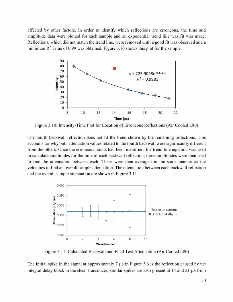
50
affected by other factors. In order to identify which reflections are erroneous, the time and
amplitude data were plotted for each sample and an exponential trend line was fit was made.
Reflections, which did not match the trend line, were removed until a good fit was observed and a
minimum R2 value of 0.99 was obtained. Figure 3.10 shows this plot for the sample.
Figure 3.10: Intensity-Time Plot for Location of Erroneous Reflections (Air Cooled L80)
The fourth backwall reflection does not fit the trend shown by the remaining reflections. This
accounts for why both attenuation values related to the fourth backwall were significantly different
from the others. Once the erroneous points had been identified, the trend line equation was used
to calculate amplitudes for the time of each backwall reflection; these amplitudes were then used
to find the attenuation between each. These were then averaged in the same manner as the
velocities to find an overall sample attenuation. The attenuation between each backwall reflection
and the overall sample attenuation are shown in Figure 3.11.
Figure 3.11: Calculated Backwall and Final Test Attenuation (Air Cooled L80)
The initial spike in the signal at approximately 7 s in Figure 3.6 is the reflection caused by the
integral delay block in the shear transducer; similar spikes are also present at 14 and 21 s from
y = 225.9098e-0.1181x
R² = 0.9981
0
10
20
30
40
50
60
70
80
90
8 10 12 14 16 18 20 22
Inte
nsi
ty
Time (s)
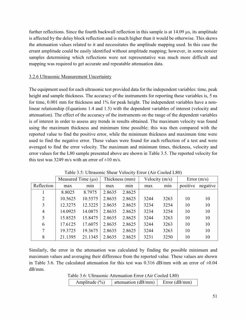
51
further reflections. Since the fourth backwall reflection in this sample is at 14.09 µs, its amplitude
is affected by the delay block reflection and is much higher than it would be otherwise. This skews
the attenuation values related to it and necessitates the amplitude mapping used. In this case the
errant amplitude could be easily identified without amplitude mapping; however, in some noisier
samples determining which reflections were not representative was much more difficult and
mapping was required to get accurate and repeatable attenuation data.
3.2.6 Ultrasonic Measurement Uncertainty
The equipment used for each ultrasonic test provided data for the independent variables: time, peak
height and sample thickness. The accuracy of the instruments for reporting these variables is, 5 ns
for time, 0.001 mm for thickness and 1% for peak height. The independent variables have a non-
linear relationship (Equations 1.4 and 1.5) with the dependent variables of interest (velocity and
attenuation). The effect of the accuracy of the instruments on the range of the dependent variables
is of interest in order to assess any trends in results obtained. The maximum velocity was found
using the maximum thickness and minimum time possible; this was then compared with the
reported value to find the positive error, while the minimum thickness and maximum time were
used to find the negative error. These values were found for each reflection of a test and were
averaged to find the error velocity. The maximum and minimum times, thickness, velocity and
error values for the L80 sample presented above are shown in Table 3.5. The reported velocity for
this test was 3249 m/s with an error of ±10 m/s.
Table 3.5: Ultrasonic Shear Velocity Error (Air Cooled L80)
Measured Time (µs) Thickness (mm) Velocity (m/s) Error (m/s)
Reflection max min max min max min positive negative
1 8.8025 8.7975 2.8635 2.8625
2 10.5625 10.5575 2.8635 2.8625 3244 3263 10 10
3 12.3275 12.3225 2.8635 2.8625 3234 3254 10 10
4 14.0925 14.0875 2.8635 2.8625 3234 3254 10 10
5 15.8525 15.8475 2.8635 2.8625 3244 3263 10 10
6 17.6125 17.6075 2.8635 2.8625 3244 3263 10 10
7 19.3725 19.3675 2.8635 2.8625 3244 3263 10 10
8 21.1395 21.1345 2.8635 2.8625 3231 3250 10 10
Similarly, the error in the attenuation was calculated by finding the possible minimum and
maximum values and averaging their difference from the reported value. These values are shown
in Table 3.6. The calculated attenuation for this test was 0.316 dB/mm with an error of ±0.04
dB/mm.
Table 3.6: Ultrasonic Attenuation Error (Air Cooled L80)
Amplitude (%) attenuation (dB/mm) Error (dB/mm)

52
wave max min max min positive negative
1 80.5 79.5 0.3 0.3 0.02 0.02
2 65.5 64.5 0.4 0.3 0.03 0.03
3 52.5 51.5 -0.6 -0.6 0.02 0.02
4 76.5 75.5 1.2 1.1 0.03 0.03
5 35.5 34.5 0.4 0.3 0.05 0.05
6 28.5 27.5 0.3 0.2 0.06 0.06
7 24.5 23.5 0.5 0.4 0.07 0.07
8 18.5 17.5
Average: 0.04 0.04
The uncertainty in time measurement is the main contributor to the uncertainty in ultrasonic
velocity. If the equipment used in the laboratory were to be used in industry, the default 10 ns
resolution would be sufficient for accurate measurements. The issue with time resolution in the
samples tested in this work is related to the thin nature of the materials being tested with industrial
equipment. The samples in this work ranged in thickness from ~0.9 mm to 3.5 mm, which is
significantly thinner than the full skelp thickness of the L80 and X70 steels, which are 9 mm and
15 mm, respectively. Figure 3.12 shows how the velocity uncertainty decreases as the sample
thickness increases, using the resolution of our equipment and an assumed velocity for the air
cooled L80 sample discussed above. The shaded region shows the range of sample thicknesses
tested, which have much higher uncertainties than samples which are 9-15 mm thick.
Figure 3.12: Ultrasonic Velocity Uncertainty vs. Sample Thickness
3.3 Pipe Skelp Through Thickness Investigation

53
Ultrasonic testing was done through the thickness of two pipe skelps to see how their ultrasonic
properties varied. X-ray diffraction (XRD) was also done through the thickness of these skelps and
compared with the ultrasonic properties.
3.3.1 Experimental Design
Investigations were carried out on samples taken through the thickness of two different pipe skelp
grades, L80 and X70. Both sections were obtained as flat skelp from production runs, which would
be further processed into pipe of their respective grade. In order to investigate these skelp samples,
24 mm x 38 mm x 1 mm thick samples were obtained through the thickness of each. To obtain
these samples, bars were first cut from each skelp along the rolling direction as illustrated in Figure
3.13.
Figure 3.13: Location of Sample Bars in Skelp
Samples were then obtained from each bar through the thickness of the skelp. Cutting was done to
minimize the length of the bar used and to keep samples as close to the same location as possible.
Figure 3.14A shows sample locations through the X70 bar and Figure 3.14B shows locations
through the L80 bar. Once cut, the samples were then surface ground to produce parallel faces and
a consistent surface finish.

54
(A)
(B)
Figure 3.14: Sample Locations Through the Thickness of (A) X70 and (B) L80 Bars.
3.3.2 XRD Analysis
The sectioned samples were characterized using X-ray Diffraction (XRD). Testing was performed
using a Rigaku rotating anode RU-200B XRD system equipped with a copper x-ray source and
graphite monochromator. The divergence slit was 1o and the monochromator slit was 0.8 mm. The
scanning range was from 10o to 110o with a 0.05o step size and 2o per minute scanning speed.
Before each set of samples was tested, a LaB6 calibration sample was run.
In order to analyze the data obtained from XRD, Rietveld refinement was done using TOPAS
Academic Software, Version 5. This software was used to obtain the spherical harmonics
coefficients for preferential orientation (Cmn), domain size (Ds) and microstrain (ε), as described
in Section 1.6, for each sample. The same software was used to obtain the instrument parameters
and calibration from the LaB6 samples. These include the error in setting the 2θ zero point
(Zero_Error), corrections for peak asymmetry due to axial divergence (Simple_Axial_Model), the
background function (bkg) and Cagliotti parameters for the instrument profile (UVW). The
background function was approximated as a sixth order or lower polynomial. In addition to the
sample data, instrument information was entered. The Lorentz-polarization (LP) factor is a
measure of the degree of polarization of the radiation, with zero being unpolarised and 90 being

55
completely polarized. For the instrument used, with a copper source and graphite monochromator,
the LP factor was 26.4. To account for the wavelength used, a factor for the source was entered,
CuK1(0.001). Figure 3.15 shows an example of a LaB6 XRD pattern.
Figure 3.15: LaB6 XRD Pattern and Instrument Parameters
From the LaB6 pattern, the 2θ zero point error was found to be 0.05639o, the peak asymmetry axial
divergence was 12.05812, the Cagliotti U, V, W parameters were 0.048, 0.369 and 0.006,
respectively, and the background function was 16.06x4-11.45x
3+6.83x
2-3.65x+2.18. Using these
instrument parameters, the steel sample parameters could be inputted and analyzed. All steel
samples were primarily ferrite; peaks were not seen or detected for any other phases. The
parameters acquired from the LaB6 calibrations were set as constants in order to find the
parameters of interest for each steel sample. A sample XRD pattern for an L80 steel sample, from
the top face of the skelp, is shown in Figure 3.16. From Rietveld fitting of the pattern, the domain
size was found to be 143 nm, the microstrain was 1.1x10⁻³ and the lattice parameter was 0.2869
nm. The spherical harmonics coefficients C41 and C61 were found to be 0.157 and -0.060,
respectively.
Figure 3.16: Sample L80 (Sample Depth of 1 mm) XRD Pattern and Obtained Parameters
Issues with sample preparation and Rietveld refinement cast doubt on the results obtained from
XRD analysis. X-rays do not penetrate deeply into the bulk of material tested but provide data only

56
for near surface material. The samples used in this work were machined and surface ground which
can create a work hardened surface layer. The XRD patterns for these samples could then be
greatly affected by this work hardened layer. In order to obtain accurate, representative diffraction
patterns from the samples, the work hardened layer would have to be removed by a process such
as electropolishing. It would also be necessary to independently verify the information obtained
from Rietveld refinement with a more direct measurement technique, such as transmission electron
microscopy, to ensure that the Rietveld quantities obtained, such as domain size and dislocation
density, are meaningful. Neither removal of the work hardened layer nor independent verification
of parameters were performed for the through thickness samples. Analysis of the results from XRD
of these samples is presented in Appendix B rather than in the main body of the thesis, because of
the uncertainty introduced by these factors.
3.3.3 Ultrasonic Tests
The samples were ultrasonically tested as described in Section 3.2 to find ultrasonic velocity and
attenuation. The ultrasonic values were then compared with the parameters found using XRD, as
well as their location through the skelp, to determine any correlations. The ultrasonic properties,
velocity and attenuation, are shown in Table 3.8 for L80 and Table 3.7 for X70 samples.
Table 3.7: X70 Through Thickness Ultrasonic Properties
Long Shear (P) Shear (T)
Sample Velocity
(m/s)
Attenuation
(dB/mm)
Velocity
(m/s)
Attenuation
(dB/mm)
Velocity
(m/s)
Attenuation
(dB/mm)
1 5968 0.30 3234 0.39 3157 0.45
2 5941 0.31 3279 0.27 3174 0.35
3 5922 0.22 3275 0.42 3174 0.55
4 5915 0.32 3273 0.41 3144 0.52
5 5936 0.30 3284 0.40 3172 0.44
6 5941 0.35 3271 0.37 3158 0.38
7 5949 0.32 3267 0.36 3117 0.53
8 5936 0.31 3279 0.48 3171 0.33
9 6018 0.50 3342 0.51 3166 0.52
10 5932 0.31 3281 0.38 3165 0.43
11 5945 0.32 3290 0.37 3169 0.40
12 5937 0.41 3294 0.36 3164 0.51
13 5920 0.36 3247 0.40 3172 0.30
14 5931 0.32 3305 0.27 3113 0.44
15 5927 0.29 3280 0.30 3155 0.33

57
Table 3.8: L80 Through Thickness Ultrasonic Properties
Long Shear (P) Shear (T)
Sample Velocity
(m/s)
Attenuation
(dB/mm)
Velocity
(m/s)
Attenuation
(dB/mm)
Velocity
(m/s)
Attenuation
(dB/mm)
1 5912 0.30 3279 0.60 3245 0.44
2 5904 0.33 3281 0.50 3256 0.54
3 5899 0.30 3274 0.56 3243 0.66
4 5904 0.33 3291 0.64 3255 0.65
5 5904 0.35 3291 0.58 3265 0.62
6 5904 0.38 3284 0.47 3246 0.69
7 5899 0.33 3282 0.55 3249 0.73
8 5894 0.29 3291 0.60 3252 0.71
9 5899 0.29 3276 0.55 3243 0.61
3.4 Interstitial Free Steel Annealing
Interstitial free steel was annealed to see how processing affected ultrasonic properties. Interstitial
free steel was chosen to simplify the analysis, since it has a low carbon content so only ferrite with
very few precipitates should form.
3.4.1 Experimental Design
To investigate the effect of annealing on ultrasonic waves, interstitial free steel was obtained in
the form of rolled sheet. Samples, 24 mm x 38 mm in size, were shear cut from the sheet so
directionality could be easily seen and to provide enough material for metallography and ultrasonic
testing. Two sets of samples were prepared. The first set was placed in a box furnace and heated
to 700oC. The samples were held at this temperature with a sample removed every five minutes
and air cooled until one hour had passed. This is shown schematically in Figure 3.17 with
approximate cooling rates.
Figure 3.17: Heat Treat Schematic of IF Samples Held at 700oC
0
100
200
300
400
500
600
700
800
0 20 40 60 80 100 120
Tem
p. (
°C)
Time (mins)

58
The second set of samples was heated to 775oC and then samples were removed every 30 minutes
and air cooled until two hours had passed. A schematic of this heat treating process is shown in
Figure 3.18.
Figure 3.18: Heat Treat Schematic of IF Samples Held at 775oC
Once heat treatment was complete and the samples were cooled to ambient temperature, a section
of each sample (~6 mm x 24 mm) was removed for metallography, using a water cooled precision
diamond saw.
3.4.2 Metallography
The sectioned samples were mounted using two part epoxy and then ground and polished using an
autopolisher; the final polishing compound was one micron diamond slurry. Etching was done
using 2% Nital followed by Marshall’s reagent. Marshall’s reagent consists of equal parts of 30%
hydrogen peroxide (Part A) and 5 mL concentrated sulfuric acid and 8 g oxalic acid mixed with
100 mL of water (Part B) [90]. Samples were immersed in the reagent for approximately thirty
seconds with the surface vertical to prevent pitting. The sizes of the grains were then observed
qualitatively to see the effect of holding time and temperature. Five microhardness indents were
performed on each of the 700oC and 775oC hold samples, with a 1 kg load and dwell time of 14 s,
using a Wilson automatic microhardness indenter. Table 3.9 shows the results of the microhardness
tests for the 700oC samples, while Table 3.10 shows the results for the 775oC samples.
Table 3.9: Microhardness of IF Steel Held at 700oC
Hold Time (min) 0 5 10 15 20 25 30 35 40 45 50 55 60
Hardness (HV1) 115 88 91 86 88 86 88 85 86 86 86 85 85
Table 3.10: Microhardness of IF Steel Held at 775oC
Hold Time (min) 0 30 90 120 160
Hardness (HV1) 83 75 76 72 72
0
100
200
300
400
500
600
700
800
900
0 50 100 150 200
Tem
p (
°C)
Time (mins)

59
3.4.3 Ultrasonic Tests
The samples were ultrasonically tested as described in Section 3.2 to determine the ultrasonic
velocity and attenuation. The ultrasonic properties are shown in Table 3.11 for the 700oC holds
and Table 3.12 for the 775oC holds.
Table 3.11: Ultrasonic Properties for IF Held at 700oC
Long Shear (P) Shear (T)
Hold Time
(min)
Velocity
(m/s)
Attenuation
(dB/mm)
Velocity
(m/s)
Attenuation
(dB/mm)
Velocity
(m/s)
Attenuation
(dB/mm)
0 6197 0.72 3160 0.70 3065 0.76
5 6284 0.97 3152 0.90 3065 1.31
10 6227 0.72 3140 0.60 3049 0.65
15 6305 0.68 3206 1.38 3081 1.13
20 6273 0.68 3156 1.07 3053 0.77
25 6292 0.65 3157 0.69 3070 0.83
30 6269 0.74 3152 0.56 3059 0.87
35 6255 1.15 3140 1.08 3061 0.89
40 6288 0.63 3156 0.95 3056 0.69
45 6312 0.87 3189 1.25 3073 1.15
50 6241 1.05 3168 0.79 3071 1.26
55 6328 0.74 3182 0.76 3083 0.70
60 6377 0.86 3204 0.93 3102 0.85
Table 3.12: Ultrasonic Properties for IF Held at 775oC
Long Shear (P) Shear (T)
Hold Time Velocity Attenuation Velocity Attenuation Velocity Attenuation
(min) (m/s) (dB/mm) (m/s) (dB/mm) (m/s) (dB/mm)
0 6294 0.78 3147 0.78 3063 0.85
30 6504 0.68 3219 0.83 3113 0.90
60 6431 0.81 3172 0.80 3057 0.81
90 6409 0.94 3144 1.13 3045 0.76
120 6445 0.90 3166 1.12 3055 1.01
3.5 L80 Steel Microstructure Variation
L80 pipe skelp was heat treated to see how changes in microstructure affected the ultrasonic
properties. Small bars were initially tested followed by longer bars, which could also be tensile
tested in addition to ultrasonic and hardness testing.

60
3.5.1 Experimental Design
To investigate the effect of microstructure on ultrasonic waves, an L80 steel, containing 0.244
wt% C and 0.99 wt% Mn among other alloying elements, was processed to obtain different
structures. Sixteen samples, 24 mm x 38 mm x 3mm thick, were machined from the skelp about
a quarter of the way through the thickness. Half of these samples were then coated in Quickrete
fireplace mortar to slow their cooling after heat treatment. All 16 samples were heated in a box
furnace to 1000oC and immediately removed. This was done to austenitize them in a manner
approximating that done to industrial L80. The samples were cooled in a variety of ways ranging
from air cooled (AC) to water quenched (WC). Table 3.13 shows the various cooling media and
sample designations.
Table 3.13: L80 Cooling Media and Sample Designations
CAC AC 200-COC 200-OC COC OC CWC WC
Quenching medium Air Air 200oC Oil 200oC Oil Oil Oil Water Water
Coating yes - yes - yes - yes -
Samples cooled in 200oC canola oil were held for three minutes and then water quenched. The oil
quenched samples used Quenchfast brand quenching oil. Figure 3.19 shows all L80 sample heat
treatments schematically, with approximate cooling rates.
Figure 3.19: L80 Small Sample Heat Treatment Schematic. Times Are Approximate.
0
100
200
300
400
500
600
700
800
900
1000
0 20 40 60 80 100 120 140 160
Tem
p. (
°C)
Time (mins)
WC
CWC
OC
COC
200-OC
200-COC
AC
CAC
FC

61
After heat treatment the samples were surface ground to remove scale and to generate parallel
faces with consistent surface roughness. They were then ultrasonically tested as detailed in Section
3.3. After ultrasonic testing, a quarter inch section of each sample was removed with a water cooled
diamond saw and mounted in epoxy. The mounted samples were ground and polished with an
autopolisher to a final polish with one micron diamond slurry and then etched with 2% Nital. The
microstructure of each sample was qualitatively evaluated using an optical microscope.
In order to obtain more statistically significant data, additional samples were tested. The samples
were rough machined from the same L80 skelp to a size corresponding to 240 mm x 20 mm x 4
mm, so that multiple ultrasonic readings could be taken from each sample, metallographic samples
could be prepared and tensile samples could be machined. In addition to the heat treatments
described in Table 3.13, furnace cooled (FC) samples were also produced with the long bars.
Samples were processed in four batches, three batches without cooling in hot oil and a fourth batch
where coated and uncoated samples were cooled in the hot oil. The time taken to heat the samples
to 1000oC ranged from 43 to 48 minutes. Figure 3.20 shows these heating profiles, the time was
measured as the furnace heated with readings taken every 50oC.
Figure 3.20: L80 Long Bar Heating Rates
After heat treatment was complete, the samples were surface ground to a thickness of 3 mm.
Approximately 20 mm was removed from either end of each sample with a water cooled diamond
saw and then the samples were cold mounted in epoxy. All mounted samples were then ground
and polished as a group to a final polish of 1 micron diamond using an autopolisher.
3.5.2 Ultrasonic Tests
0
200
400
600
800
1000
0 10 20 30 40 50
Tem
p. (
C)
Time (mins)
Round 1
Round 2
Round 3
Hot Oil

62
The small samples were ultrasonically tested as described in Section 3.2 to determine ultrasonic
velocity and attenuation. The ultrasonic properties, velocity and attenuation, are shown in Table
3.14.
Table 3.14: L80 Small Bar Heat Treated Ultrasonic Properties
Long Shear (T)
Sample Velocity
(m/s)
Attenuation
(dB/mm)
Velocity
(m/s)
Attenuation
(dB/mm)
Coated - Air Cooled 5893 0.258 3258 0.356
Air Cooled 5905 0.250 3249 0.316
Coated - 200 C Oil Quench 5893 0.263 3245 0.199
200 C Oil Quench 5913 0.268 3232 0.317
Coated - Oil Quench 5895 0.252 3215 0.243
Coated - Water Quenched 5900 0.230 3199 0.293
Oil Quench 5895 0.258 3208 0.319
Water Quenched 5895 0.245 3194 0.261
The long bar samples were tested in the same manner as the small samples, but three readings were
taken from each bar and the values for each heat treatment (three bars) were averaged to get the
ultrasonic velocity. The standard deviation of the readings was taken as the error rather than the
calculated instrument error used for single readings. The average ultrasonic properties are shown
in Table 3.15 along with the standard deviations in Table 3.16.
Table 3.15: L80 Long Bar Heat Treated Ultrasonic Properties
Long Shear (P) Shear (T)
Sample Velocity
(m/s)
Attenuation
(dB/mm)
Velocity
(m/s)
Attenuation
(dB/mm)
Velocity
(m/s)
Attenuation
(dB/mm)
Furnace Cooled (FC) 5896 0.25 3254 0.35 3266 0.34
Coated - Air Cooled 5900 0.24 3268 0.28 3285 0.29
Air Cooled 5897 0.20 3261 0.30 3275 0.28
Coated - 200 C Oil Quench 5908 0.18 3244 0.25 3253 0.25
200 C Oil Quench 5908 0.18 3236 0.23 3247 0.24
Coated - Oil Quench 5904 0.17 3220 0.23 3224 0.22
Coated - Water Quenched 5894 0.16 3207 0.23 3214 0.22
Oil Quench 5900 0.17 3207 0.23 3213 0.26
Water Quenched 5916 0.17 3215 0.25 3215 0.24
Table 3.16: L80 Long Bar Standard Deviation of Ultrasonic Properties
Long Shear (P) Shear (T)

63
Sample Velocity
(m/s)
Attenuation
(dB/mm)
Velocity
(m/s)
Attenuation
(dB/mm)
Velocity
(m/s)
Attenuation
(dB/mm)
Furnace Cooled 2 0.01 6 0.03 3 0.04
Coated - Air Cooled 9 0.00 7 0.00 6 0.03
Air Cooled 6 0.02 5 0.03 5 0.04
Coated - 200 C Oil Quench 9 0.01 6 0.01 7 0.02
200 C Oil Quench 5 0.01 7 0.03 7 0.02
Coated - Oil Quench 12 0.02 11 0.03 14 0.02
Coated - Water Quenched 6 0.01 10 0.05 4 0.03
Oil Quench 8 0.01 5 0.01 6 0.05
Water Quenched 29 0.01 17 0.06 19 0.06
3.5.3 Vickers Hardness
Microhardness tests were obtained using a manual Vickers hardness indenter with a 500 g load.
Three to five indents were done on each sample, depending on measurement variation. The values
were averaged to determine the hardness of the sample. Both the hardness and heat treatment were
then compared with the ultrasonic properties measured. The microhardness values for each sample
are shown in Table 3.17.
Table 3.17: L80 Small Bar Microhardness
Sample Average Hardness
(HV0.5)
Standard Deviation
(HV0.5)
Coated - Air Cooled 177 2
Air Cooled 200 21
Coated - 200 C Oil Quench 230 20
200 C Oil Quench 349 8
Coated - Oil Quench 455 24
Coated - Water Quenched 526 25
Oil Quench 490 39
Water Quenched 485 28
Microhardness was also done on the polished samples sectioned from the long bars. These samples
were indented with a Wilson VH3100 automatic microhardness tester. A load of 1 kg and a dwell
time of 14 seconds were used for each of the 15 Vickers hardness indents made on each sample.
The automatic microhardness tester measured each indent and calculated the resultant Vickers
hardness. The average of all the hardness tests done for each heat treatment was calculated and the
standard deviation used as the error. These values are shown in Table 3.18.

64
Table 3.18: L80 Long Bar Microhardness
Sample Average Hardness
(HV1)
Standard Deviation
(HV1)
Furnace Cooled 140 5
Coated - Air Cooled 166 4
Air Cooled 178 5
Coated - 200 C Oil Quench 281 24
200 C Oil Quench 306 8
Coated - Oil Quench 433 8
Coated - Water Quenched 433 7
Oil Quench 465 24
Water Quenched 513 13
3.5.4 Metallography
Once hardness tests were completed, the samples taken from the long bars were etched with 2%
Nital and their microstructures viewed optically. One way of assessing the microstructures was by
measuring grain size. This was done in accordance with ASTM E112 - Standard Test Methods for
Determining Average Grain Size [91]. To measure grain size, a circle of known perimeter was
overlaid on micrographs taken from each sample. The number of times the circle crossed a grain
boundary was counted and the grain size calculated as the length of the circle divided by the
number of intercepts. Figure 3.21 shows an example of such a circle and a micrograph; the grain
size was measured as 88 μm.
Figure 3.21: Circle Overlay for Grain Size Measurement of a Furnace Cooled (FC) Sample

65
This process was repeated for 9-30 fields of view on each heat treatment; the number depended on
the ability to resolve individual grains at low magnification. For the FC, CAC, and AC samples
grain size was measured, however in the remaining samples the colony size was measured as the
grains could not be distinguished from one another (See Appendix A for further information). The
values were averaged to get a grain size for each heat treatment. The grain sizes are shown in Table
3.19.
Table 3.19: L80 Long Bar Grain or Colony Sizes
Sample
Grain/
Colony Size
(μm)
Standard Deviation
(μm)
Furnace Cooled 72 55
Coated - Air Cooled 40 27
Air Cooled 81 44
Coated - 200 C Oil Quench 48 12
200 C Oil Quench 72 10
Coated - Oil Quench 66 19
Coated - Water Quenched 89 29
Oil Quench 81 21
Water Quenched 86 28
Quantitative phase analysis was also done on optical micrographs where possible. This was done
by overlaying a grid of points on the micrograph in accordance with ASTM E562 – Standard Test
Method for Determining Volume Fraction by Systematic Manual Point Count [92]. The fraction
of points located in a phase is indicative of the area fraction of that phase in the micrograph. This
analysis was only possible on samples which were cooled slowly. Those cooled quickly did not
show enough of a second phase to allow for analysis. Figure 3.22 shows a sample grid overlay and
phase fraction.

66
Figure 3.22: Grid Overlay for Phase Fraction Measurement of a FC Sample
In this case, the dark regions are pearlite and the light regions are ferrite. At higher magnification
the dark regions showed a lamellar structure characteristic of pearlite, as well no martensite was
seen in the samples with pearlite. The point count method of the image in Figure 3.22 yielded a
microstructure fraction of 46% pearlite and 54% ferrite. This procedure was repeated for at least
14 micrographs of each of the furnace and air cooled sets. These heat treatments had clearly
defined microstructures which could be differentiated, unlike the more rapidly cooled samples. In
the martensitic samples it could not be determined optically if specific regions were martensite or
not. The values from each field of view were averaged to get representative values, which are
given in Table 3.20.
Table 3.20: L80 Long Bar Phase Fraction
Sample Area %
Pearlite
Area %
Ferrite
Standard Deviation
(%)
Furnace Cooled 48 52 18
Coated - Air Cooled 40 60 13
Air Cooled 41 59 13
3.5.5 Tensile Tests
After the ends of each sample were removed, the remainder of the sample was machined into a
tensile dog bone sample in accordance with ASTM E 8M-04 – Standard Test Methods for Tension
Testing of Metallic Materials [93]. The sample dimensions from the specification are shown in
Figure 3.23.

67
Figure 3.23: Tensile Test Sample Dimensions [93]
The tensile specimens were tested to failure with an Instron 8516 Loading Frame equipped with
Instron 2743 100KN hydraulic wedge grips, an Instron 8800 controller and a 12.5 mm gauge length
extensometer, which was attached to the specimens with elastic bands. The cross sectional area in
the reduced section (W and T in Figure 3.23) of each specimen was measured prior to testing with
a micrometer in the same manner as used prior to ultrasonic testing. The tensile test was conducted
at a displacement rate of 3 mm/min. The extensometer generates a strain value in volts, which is
converted to mm/mm using Equation 3.1 where εmm/mm is the strain in mm/mm, ε is the
extensometer output in volts and G is the gauge length of the extensometer (12.5 mm) [94].
휀𝑚𝑚/𝑚𝑚 = (𝜀𝑉
2) 𝐺⁄ (3.1)
The stress was calculated using the output force measured by the instrument divided by the original
cross sectional area. The resulting engineering stress was plotted as a function of engineering
strain; an example of a stress-strain plot is shown in Figure 3.24 for the air cooled specimen that
was heated in the first round (AC1).
Figure 3.24: Stress-Strain Plot for AC1 L80 Specimen
0
100
200
300
400
500
600
700
0 0.02 0.04 0.06 0.08 0.1
Stre
ss (
MP
a)
Strain (mm/mm)

68
The Young’s modulus was measured by fitting a trend line to the linear portion of the stress-strain
curve. Points were removed from the curve until a linear trend line fit well with a good R2 value
(above 0.9) and the initial and final points considered did not deviate from the trend by more than
10 MPa. This ensured that the same criteria were met for all tests and only the linear portion of the
curve was considered to find the slope. The slope of the trend line corresponds to the Young’s
modulus for the sample. Figure 3.25 shows this trend line for the AC1 specimen.
Figure 3.25: Trend Line for Determination of Young’s Modulus of AC1 Specimen
The Young’s modulus was calculated to be 194 GPa for the AC1 specimen. The Young’s modulus
for ferrite-pearlite has been reported as ~210 GPa and ~204 GPa for martensite in a 1050 steel
[82]. The Young’s modulus was then used to generate a 0.2% strain offset line to find the yield
stress of the sample [93]. The stress at which the 0.2% offset line intersected the stress-strain curve
was taken to be the yield strength (YS) of the sample. Figure 3.26 shows the two curves and their
intersection.
y = 194239x - 5.8807R² = 0.9987
0
50
100
150
200
250
0 0.0002 0.0004 0.0006 0.0008 0.001 0.0012 0.0014
Stre
ss (
MP
a)
Strain (mm/mm)

69
Figure 3.26: Stress-Strain Curve and 0.2% Offset Line for Yield Strength (YS) Determination
AC1 Specimen
The 0.2% offset method for the AC1 sample generated a yield strength of 385.1 MPa. This value
was compared with the average stress in the plateau region of the stress-strain curve (384.9 MPa),
which is an alternative method for measuring yield strength in samples with a plateau in their
stress-strain curve. The value using the 0.2% offset method was taken as the yield strength for the
sample, since it agreed with the plateau method and could be used consistently on all samples,
including those without plateaus. The Young’s modulus was used to determine the elongation of
the sample. The intercept of a line with slope equal to the Young’s modulus with the strain axis
was adjusted until it intersected the stress strain curve at the point of fracture. The strain intercept
of this line was the elongation of the sample. A vertical line was also placed at this point to find
the fracture strain. By using a line with slope equal to the Young’s modulus the elastic portion of
the fracture strain was removed to give the elongation for the sample. Both lines are shown in
Figure 3.27.
Figure 3.27: Fracture Strain and Elongation Determination
0
50
100
150
200
250
300
350
400
450
500
0 0.002 0.004 0.006 0.008 0.01 0.012 0.014
Stre
ss (
MP
a)
Strain (mm/mm)
0
100
200
300
400
500
600
700
0.0975 0.1 0.1025 0.105
Stre
ss (
MP
a)
Strain (mm/mm)
Stress-Strain
Fracture Strain
Elongation

70
The fracture strain for this sample was 10.25% and the elongation was 9.95%. The fracture strain
was used as a cut-off value when finding the area below the stress strain curve. To determine the
area under the curve, the area of the trapezoid between each sequential pair of points and the x-
axis was found by adding the area of the rectangle between the lower point, it’s y-coordinate with
the x-coordinate of the upper point and the x-axis to the triangle formed by the upper point and the
top of the rectangle. The areas of all these trapezoids was summed up until the breaking strain was
reached. These areas were then summed to get a value for the toughness of each sample. A
simplified schematic of this method showing eight points rather than the full 2385 is shown in
Figure 3.28 for the AC1 sample.
Figure 3.28: Trapezoid Method for Finding Area Under The Stress Strain Curve
For the AC1 sample (Figure 3.22) the toughness was 35 MJ/m3. The ultimate tensile strength
(UTS) was also calculated by finding the maximum value for stress among the data points for the
sample. The AC1 sample had a UTS of 610 MPa. This process was repeated for all 27 heat treated
tensile specimens and the values are shown in Table 3.21.
Table 3.21: L80 Tensile Test Results
Sample Y (GPa) YS
(MPa)
UTS
(MPa)
Fracture
Strain
(%)
Elongation
(%)
Toughness
(MJ/m3)
Furnace Cooled 197 298 537 27 27 65
Coated - Air Cooled 200 365 583 23 23 62
Air Cooled 197 380 604 13 13 43
Coated - 200 C Oil Quench 203 655 830 4 3 18
200 C Oil Quench 202 725 910 3 3 18
Coated - Oil Quench 197 849 1145 8 7 30
Coated - Water Quenched 200 1059 1497 9 9 47
Oil Quench 206 1149 1588 7 6 50
Water Quenched 199 1158 1602 4 4 45
0
200
400
600
800
0 0.02 0.04 0.06 0.08 0.1 0.12
Stre
ss (
MP
a)
Strain (mm/mm)

71
3.6 Industrial UT
Further tests were done with two commercially available steels with equipment and practices used
in industry. 4130 was chosen as it can be treated into an L80 steel and should be comparable to the
L80 tested previously while 5160 was procured as a production part which was not a rolled skelp
like the other steels tested.
3.6.1 5160 and 4130 Experimental Design
Experimentation was conducted on 4130 and 5160 alloy steels similar to that done on the L80
small bars. The higher carbon contents of these steels facilitated the creation of differing
microstructures. Eight samples, roughly 24 mm x 24 mm in size, were cut from a 5160 leaf spring
using an abrasive cutting wheel. The samples were ground flat after sectioning, since the original
leaf spring was curved. This resulted in a loss of thickness compared with the original spring; as
such, each sample had a unique thickness. This is evident in Figure 3.29. The final thickness of
the 5160 samples ranged from approximately 6.5-8 mm.
Figure 3.29: Schematic of Samples Taken from 5160 Leaf Spring
Nine 4130 samples, roughly 24 mm x 24 mm in size, were cut from commercially available 12
mm thick bar stock. Since the bar already had uncurved parallel faces, no thickness reduction was
needed. Both sets of samples were subjected to a variety of heat treatments, beginning with a one
hour austenization at 845oC, to produce different microstructures including martensite, by
quenching in water (Q), tempered martensite, by quenching and tempering at 650oC (QT1) or
205oC (QT2), fine pearlite, by air cooling (AC), and coarse pearlite by furnace cooling (FC). In
addition, three methods to obtain spheroidized carbides were attempted by holding the samples at
770oC for 6 hrs (H1) or 69 hrs (H2) after austenization or 16 hrs without austenization (H3). Figure
3.30 shows the heat treatments schematically with approximate cooling rates.

72
(A)
(B)
Figure 3.30: 5160 and 4130 Heat Treatments; (A) Short times and (B) High Temperature Holds
3.6.2 5160 and 4130 Ultrasonic Tests
Once the samples were heat treated, they were taken to UT Quality to have their ultrasonic shear
wave velocities measured. Measurements were done with a Krautkramer USN58L pulser/receiver
and a 15 MHz 0o shear wave piezoelectric transducer with stabilized molasses as a couplant. This
equipment is standard in industry. The sample thickness was measured using a digital caliper. The
couplant was put on the transducer and then spread using a small clamp to affix the transducer to
the sample. The transducer and signal gain were simultaneously adjusted until the signal from the
first backwall reflection was at 80% of the display screen height, which is the standard procedure
for flaw detection [95]. The velocity of each sample was obtained by adjusting a pre-set velocity
in the pulser/receiver software until the first two backwall reflection distances matched the
0
100
200
300
400
500
600
700
800
900
0 10 20 30 40 50 60 70
Tem
p. (
°C)
Time (hrs)
H1
H2
H3

73
measured sample thickness. If a sample was measured to be 3 mm thick, the first backwall
reflection would be displayed as 3 mm while the second reflection would be 6 mm away. The input
velocity, which resulted in the reflections matching the measured thickness, was then the ultrasonic
shear wave velocity in the sample. An example is shown in Figure 3.31.
Figure 3.31: Krautkramer Ultrasonic Velocity Test
Since the resolution of the time measurement within the instrument was not known, only the error
from the thickness measurement, ±0.01 mm, was considered. This procedure was followed to
ultrasonically test all samples. The results of these tests are shown in Table 3.22.
Table 3.22: Industrial UT Results for 4130 and 5160
Velocity (m/s)
Sample 4130 5160
As Received 3219 3175
Quenched 3172 3157
Quench - Temper @ 650oC 3220 3148
Quench - Temper @ 205oC 3204 3129
Air Cool 3209 3288
Furnace Cool 3212 3200
High Temp. Hold 1 -770oC for 6hrs 3224 3205
High Temp. Hold 2 – 770oC 69hrs 3219 3183
High Temp. Hold 3 – 770oC 16.5hrs - no
normalize 3105 -
Once ultrasonic testing was completed, the samples were prepared for optical microscopy to view
the through thickness microstructure in each sample. Samples were cut using a water cooled

74
abrasive saw and then cold mounted in two part epoxy. Grinding and polishing was done by hand,
down with one micron diamond slurry as the final step. The samples were microhardness tested in
the same manner as the L80 long bar samples but with the five indents oriented through their
thickness. The results of these hardness tests are shown in Table 3.23. The samples were then
etched with 2% Nital and images were taken with an optical microscope at varying magnifications
for qualitative analysis of the microstructure.
Table 3.23: 5160 and 4130 Microhardness
5160 4130
Heat
Treatment
Hardness
(HV1)
Standard
Deviation
Hardness
(HV1)
Standard
Deviation
Q 702 28 567 10
AC 388 15 258 45
AR 540 15 233 8
FC 290 9 163 7
QT1 362 14 258 14
Qt2 659 34 526 10
H1 389 13 169 6
H2 252 7 158 3
H3 - - 189 5
3.7 Summary of Experimental Methods and Results
Experimental work was conducted through the thickness of pipe skelps with UT and XRD, on IF
steel cooled to room temperature after different annealing times with UT and microhardness, L80
steel after different heat treatments with UT, microhardness, tensile tests, and optical microscopy
and 5160 and 4130 steel after heat treatment with UT and microhardness. The pipe skelps used for
through thickness investigation were L80 and X70. UT and XRD were done on 1 mm thick
samples obtained through the thickness of each skelp. The ultrasonic velocity and attenuation for
shear and longitudinal waves was also obtained. Discussion of the ultrasonic properties and
location through the skelps are presented in Section 4.1. The annealed IF steel shear and
longitudinal wave velocity and attenuations as well as microhardness were obtained at room
temperature after cooling from different times and annealing temperatures. Discussion regarding
the IF steel and its ultrasonic properties after different amounts of annealing is given in Section
4.2. The L80 steel samples which were austenitized then cooled at different rates to obtain different
microstructures are discussed in Section 4.3. Ultrasonic velocity and attenuation for shear and
longitudinal waves as well as microhardness, Y, YS, UTS, fracture strain, elongation, and
toughness were found for the different L80 heat treatments used. Heat treatments were also done
to 5160 and 4130 samples to obtain different microstructures. The ultrasonic shear and longitudinal
wave velocity and attenuation were obtained for these heat treatments as well as the microhardness,
the discussion of which can be found in Section 4.4.

75
Chapter 4 Discussion
The tabulated ultrasonic results found in the previous chapter are compared with materials
properties, processing and microstructure. The ultrasonic properties of two pipe skelps, L80 and
X70, are compared with the domain size, microstrain, dislocation density and texture index found
using quantitative XRD as well as their location through the thickness of the skelp. This was done
to see if the ultrasonic properties changed through the thickness of the skelp and if the correlated
to the information obtained from quantitative XRD. The ultrasonic properties of the annealed IF
steels are compared with the hold times at high temperature and the resultant hardness values to
see how ultrasonic properties varied as annealing progressed. The ultrasonic properties of the heat
treated L80 samples are compared with the heat treatment procedure, hardness values and material
properties from tensile tests to see if changes in morphology and structure affect the ultrasonic
properties. The ultrasonic properties of the 4130 and 5160 heat treated samples were also compared
with the heat treatment and hardness values to see if changes in structure could be detected with
industrial equipment and procedures.
4.1 Pipe Skelp Through Thickness Investigation
Pipe skelps for two different grades of pipe, L80 and X70, were ultrasonically tested and the results
compared with materials properties gathered through XRD. The ultrasonic properties through the
skelp thickness were also compared with one another to see if any significant variation occurred
through the skelp. They were also compared with the calculated velocities found in Section 2.2.
Rietveld refinement of XRD patterns was used to find the texture index (J) of each sample as well
as the dislocation density, microstrain and domain size. These were then compared with the
ultrasonic properties.
4.1.1 Ultrasonic Velocity Through Skelp Thickness
The ultrasonic velocity through the thickness of each skelp was analyzed. The velocities were also
compared with those calculated using the anisotropic method in Section 2.2.
4.1.1.1 X70 Through Thickness Velocity
The ultrasonic velocities through the thickness of the X70 skelp did not show significant variation
(Figure 4.1). While there was some scatter in the velocities, including a significant spike upwards
in both the longitudinal (VL) and shear waves parallel to the rolling direction (VsP) for the sample
at a depth of 9 mm, the velocities largely remained constant throughout the thickness of the X70
skelp.

76
(A) (B)
Figure 4.1: Shear (A) and Longitudinal (B) Velocities Through X70 Skelp
The consistency in velocity is desirable for flaw detection applications. If there was significant
variation in velocity through the skelp, accurate location and sizing of flaws would be greatly
complicated. In addition, consistency in velocity points towards consistency in microstructure and
mechanical properties through the skelp. Qualitatively the microstructure appeared consistent
through the skelp with optical microscopy (Figure 4.2). The micrographs taken from the center of
the skelp appear very similar to those at the top or bottom surfaces in both the rolling direction and
transverse direction. This agrees with the velocity results and suggests that there is little centerline
segregation if any.
There is no overlap in velocity between the three wave modes. The shear waves have much lower
velocities than the longitudinal waves. The longitudinal wave velocities (VL) average 5941 m/s,
while the transverse oriented shear waves (VsT) average 3158 m/s and the shear waves oriented
along the rolling direction (VsP) average 3280 m/s.
3050
3100
3150
3200
3250
3300
3350
3400
0 3 6 9 12 15
Vel
oci
ty (
m/s
)
Sample Depth (mm)
5800
5850
5900
5950
6000
6050
6100
0 3 6 9 12 15
Vel
oci
ty (
m/s
)
Sample Depth (mm)
VL
VsP
VsT

77
(A) (B)
Figure 4.2: X70 Skelp Through Thickness Optical Images Showing Consistency In
Microstructure with: (A) Brightfield, Rolling Direction and (B) Direct Interference Contrast,
Transverse Direction. Etched with 3% Nital
Only the transverse oriented shear waves match the isotropic velocity calculations done in Section
2.2. The longitudinal velocity is much higher than the calculated value, i.e., 5941 m/s vs roughly
4600 m/s, which further confirms that the isotropic assumption is not sufficient to accurately

78
represent ultrasonic behavior. All the velocities fall within the range of velocities for each wave
type calculated in Section 2.2 for anisotropic ferrite in 1050 steel. The longitudinal waves agree
with velocities calculated for the longitudinal velocity (V1), as shown in Figure 4.3. The
longitudinal velocities fall very close to the average calculated longitudinal velocities (V1avg),
which indicates that there is very little preferential orientation in the sample. If significant
preferential orientation was present, favouring directions with velocities far from the average, the
velocities would be closer to the maximum or minimum calculated values (V1max) and (V1min).
The shear wave comparisons with calculated values are shown in Figure 4.4.
Figure 4.3: X70 Longitudinal Velocities and Calculated V1
(A) (B)
Figure 4.4: X70 Shear Velocities and Calculated (A) V2 and (B) V3
5000
5200
5400
5600
5800
6000
6200
6400
6600
6800
0 5 10 15
Vel
oci
ty (
m/s
)
Sample Depth (mm)
VL
V1 max
V1 avg
V1 min
2500
2700
2900
3100
3300
3500
3700
3900
4100
4300
0 5 10 15
Vel
oci
ty (
m/s
)
Sample depth (mm)
VsP
VsT
V2 max
V2 avg
V2 min
3000
3200
3400
3600
3800
4000
4200
0 5 10 15
Vel
oci
ty (
m/s
)
Sample depth (mm)
VsP
VsT
V3 max
V3 avg
V3 min

79
VsP falls within the range for both V2 and V3, the calculated shear velocities, while VsT falls
within the range of only V2. Since VsT is not within the range for V3, it can be assumed that VsP
is analogous with V3 and not V2. VsT velocities are near the average for V2, but not as close as the
longitudinal wave velocities are to V1, similarly indicating that there should not be much
preferential orientation in the skelp. The VsP velocities averaged only slightly above the minimum
values for V3. In order for the velocity to be that low, the grains would almost all have to be
oriented along the <111> direction. If the other velocities also deviated greatly from the average,
this hypothesis could be possible; however, the other velocities were much closer to the average
values than the minimum values. It is possible that the difference in behaviour is, instead, due to
differences in the X70 steel composition and morphology, which is a low carbon rolled product,
and the 1050 steel used in calculations, which is a medium carbon, normalized steel [82]. Each
velocity may not be equally sensitive to these changes. While V1 and V2 appear to agree very well
with the X70 velocities, V3 may be more sensitive and show different velocities from the calculated
ones.
4.1.1.2 L80 Through Thickness Velocity
As with the X70 skelp, the L80 steel also did not show significant variation in ultrasonic velocity
through the thickness of the skelp. The variation present in the L80 skelp was less than that for
X70, with no significant outliers outside the margins of error. In addition, the velocities all agreed
within error with the corresponding velocity through the entire skelp thickness taken at one time.
This can be seen in Figure 4.5, where the lines across each graph are the full thickness velocities
and the points represent the individual samples at 1 mm depth intervals.
(A) (B)
Figure 4.5: Shear (A) and Longitudinal (B) Velocities Through L80 Skelp
3050
3100
3150
3200
3250
3300
3350
3400
0 3 6 9
Vel
oci
ty (
m/s
)
Sample Depth (mm)
5800
5850
5900
5950
6000
6050
6100
0 3 6 9
Vel
oci
ty (
m/s
)
Sample Depth (mm)
VL
VsP
VsT
VL Full
VsP Full
VsT Full

80
This is again desirable for flaw detection applications, as well as indicating good consistency in
properties through the skelp. Unlike the X70 skelp, the L80 shear velocities, VsP and VsT, are
within the error range for one another. The L80 skelp also showed good consistency of
microstructure through the skelp with optical microscopy (Figure 4.6)
(A) (B)
Figure 4.6: L80 Skelp Through Thickness Optical Images Showing Consistency In
Microstructure along: (A) Rolling Direction (B) Transverse Direction. Etched with 3% Nital

81
The longitudinal waves were slower in L80 than in X70 with an average of 5902 m/s, but both
shear wave velocities were faster with average velocities of VsP 3283 m/s and VsT 3251 m/s. All
three wave types correspond to the calculated velocities in the same manner as they did for the
X70 skelp, where VL is V1, VsT is V2 and VsP is V3. The comparison of VL and V1 is shown in
Figure 4.7.
Figure 4.7: L80 Longitudinal Velocities and Calculated V1
The longitudinal velocities are lower than those found in X70 and are slightly further from the
average calculated value. They are still, however, relatively close to the average value which
suggests minimal texture effect. The shear velocities also agree with calculated values, as shown
in Figure 4.8.
(A) (B)
Figure 4.8: L80 Shear Velocities and Calculated (A) V2 and (B) V3
5000
5200
5400
5600
5800
6000
6200
6400
6600
6800
0 3 6 9
Vel
oci
ty (
m/s
)
Sample depth (mm)
VL
V1 max
V1 avg
V1 min
2500
2700
2900
3100
3300
3500
3700
3900
4100
4300
0 3 6 9
Vel
oci
ty (
m/s
)
Sample depth (mm)
VsP
VsT
V2 max
V2 avg
V2 min
3000
3200
3400
3600
3800
4000
4200
0 3 6 9
Vel
oci
ty (
m/s
)
Sample depth (mm)
VsP
VsT
V3 max
V3 avg
V3 min

82
In the L80 skelp, the shear values are all closer to the average calculated ones than in the X70 steel.
As with X70, VsT agrees well with V2, while VsP is only just inside the range of V3. The shear
values are so far from the average V3 values, which again suggests that there is some orientation
effect, but this is not borne out in the V1 and V2 results. Since both L80 and X70 are rolled products
and the calculations were done with values obtained from a normalized sample [82], it is possible
that the rolling process affected the structure in such a way that V3 is more sensitive than the other
velocities.
4.1.2 Through Thickness Attenuation
The attenuation was also found through the thickness of each skelp sample to see if there was any
variation. In the X70 skelp there was little variation through the skelp thickness or among wave
types. Figure 4.9 shows the attenuations through the X70 skelp, where AL is the longitudinal
attenuation, AsP is the shear attenuation parallel to the rolling direction and AsT is the transverse
attenuation.
Figure 4.9: Attenuation Through X70 Skelp
The attenuation of the three wave types are not distinct from one another through the X70 skelp.
For a given sample any of the three types could have the minimum attenuation at a given depth.
The shear attenuations are normally higher, which could be due to the thick couplant that does not
disperse as evenly or easily as the longitudinal couplant; however, this does not explain why the
longitudinal attenuation is not consistently the minimum value. It is also noteworthy that both the
AsP and AL have a distinct increase in attenuation for the sample at a depth of 9 mm. This same
sample also had increases in VsP and VL at the same depth. None of the three wave types show
any trend in their attenuation through the skelp. All show scatter around the average attenuation,
i.e., 0.33 dB/mm for AL, 0.38 dB/mm for AsP and 0.43 dB/mm for AsT. This scatter is significant
0.00
0.10
0.20
0.30
0.40
0.50
0.60
0.70
0 3 6 9 12 15
Att
enu
atio
n (
dB
/mm
)
Sample Depth (mm)
AL
AsP
AsT

83
enough to make it unlikely that the detected wave type could be determined the attenuation value.
This is unlike the L80 skelp, where the longitudinal attenuation, AL, is lower than the shear
attenuations in all cases (Figure 4.10).
Figure 4.10: Attenuation through L80 Skelp
The shear attenuations, AsP and AsT, overlap with the longitudinal attenuation, AL, for one case
each. For the rest of the samples, the longitudinal and shear attenuations are distinct. The lower
longitudinal attenuation could again be attributed to couplant effects. This is more likely in L80
compared with X70, since the longitudinal attenuation is consistently lower than the shear
attenuations in L80. There are no significant spikes in any of the L80 attenuations and the values
are consistent through the skelp, especially the AL attenuations since all the values are within the
error of one another. The attenuation was also determined through the whole skelp at one time,
rather than through each sample individually. The attenuations were significantly lower than those
in the individual samples; 0.19 dB/mm for AL, 0.2 dB/mm for AsP and 0.26 dB/mm for AsT.
Again this is attributed to couplant effects, since on a per mm basis the couplant will have a greater
effect for a 1 mm sample than a 9 mm sample. The difference between individual sample
attenuations and full thickness values was less for the longitudinal case than for the shear case,
again likely because of the high viscosity of the shear couplant.
Both velocity and attenuation in L80 and X70 skelps indicate little variation in the properties of
either skelp. The velocities agree with those calculated and suggest little preferential orientation is
present. The VsP was far from the average calculated V3, but remained within the range of possible
values. The difference between V3 and VsP is attributed to the difference in composition and
morphology of ferrite in the skelp samples and the normalized sample used to calculate V3. The
attenuations did not show significant variation through the skelp. For X70, attenuation was
scattered amongst the three wave types, whereas for L80 the longitudinal attenuation was lower
than the shear attenuations.
0.20
0.30
0.40
0.50
0.60
0.70
0.80
0.90
0 3 6 9
Att
enu
atio
n (
dB
/mm
)
Sample Depth (mm)
AL
AsP
AsT

84
4.1.3 Pipe Skelp Through Thickness Summary
The ultrasonic velocity and attenuation through the skelp thickness of the L80 and X70 steels did
not show significant variation. Velocities agreed with those calculated in Section 2.2 for samples
with no texture. The agreement was worse for V3 (2nd shear mode) than for V2 shear or V1
longitudinal waves. In order to better understand how the ultrasonic properties are affected by
microstructure further investigation was needed. This was done by annealing IF steel, chosen since
only ferrite forms on air cooling, to see the effect of recrystallization and grain growth on ultrasonic
properties and L80 steel after heat treatment to see the effect of forming different microstructures
such as ferrite-pearlite or martensite.
4.2 Annealing Interstitial Free Steel
Interstitial free steel was annealed at 700oC and 775oC to see the effect on ultrasonic properties.
Samples were held at 700oC for up to an hour or 775oC for up to two hours. The resultant ultrasonic
properties were compared with the holding time at each temperature, as well as the hardness of
each sample.
4.2.1 Effect of Holding Time on Microstructure
The effect of hold time on microstructure was investigated for both 700oC and 775oC holding
temperatures. Samples were polished and etched for optical microscopy. Difficulties in etching
did not allow for quantitative metallography of grain size. Hardness tests were then done to obtain
quantitative differences between samples.
4.2.1.1 700oC Holding Temperature
The interstitial free (IF) steel was held at 700oC for up to an hour to increase the grain size. Etching
proved to be extremely difficult for these samples. Nital did not etch the samples well; long etching
times were needed and Nital selectively etched some grain boundaries, but not others, making
analysis of the micrographs difficult. A sample micrograph only etched with Nital is shown in
Figure 4.11.
Figure 4.11: IF Sample Heated at 700oC for 0 Min, Etched in Nital for 5 Min

85
Some grain boundaries are quite distinct, others are faint and some do not show up at all.
Marshall’s reagent was chosen as a second etch, since it is often used for low carbon steels to etch
ferrite boundaries when Nital does an incomplete job [96]. Marshall’s reagent consists of two parts;
part A is 5 mL of concentrated sulfuric acid added to 100 mL of water followed by 8 g of oxalic
acid. Part B is 30% hydrogen peroxide which is combined in equal volume with part A. Marshall’s
reagent was found to be ineffective when used alone, but performed much better after a Nital etch
was used to remove any passive layer present on the sample. Figure 4.12 shows the as received
(AR) IF sample, along with samples heated to 700oC for 0-60 minutes.
Figure 4.12: IF Steel, Heated to 700oC for 0-60 Min, Etched in Nital and Marshall’s Reagent
It should be noted that Marshall’s reagent was more effective etching the IF steel when a mixture
using only 80% of the recommended volume of hydrogen peroxide. Both 40% sulfuric acid and
95% sulfuric acid were tested; the 40% solution produced better results. The addition of oxalic
acid prior to the sulfuric acid also improved etching response. The micrographs taken after
Marshall’s reagent etching show much better grain boundary etching, but there are still many
boundaries which are not completely etched. The micrographs are then only useful for qualitative
examination, since quantitative metallography for grain size is only accurate if all the grain
boundaries are clearly visible. The 0 and 5 minute holds should have smaller grain size, while the

86
60 minute hold should have a larger grain size. Qualitative analysis of the micrographs in Figure
4.12 do not show a significant change in grain size. The 5 and 60 minute holds appear to be quite
similar, with possibly a higher area fraction of large grains in the sample with longer hold time.
Approximate grain sizes were measured using the procedure described in Section 3.5.4 from the
best fields of view of the polished and etched samples. The results are given in Table 4.1 and show
that the grain size did not change significantly from 0 to 60 minutes of holding.
Table 4.1: Grain Size For IF Samples Held at 700oC
Sample Hold Time (mins) Grain Size (μm)
AR 7
0 12
5 11
60 12
Microhardness was then done to see if a quantitative difference could be determined between the
samples. The hardness change as a function of holding time is shown in Figure 4.13.
Figure 4.13: Hardness vs. 700oC Hold Time
The 0 min hold has the highest hardness by a large margin, while the remaining samples show
similar hardness which slightly decreases from approximately 90 HV to 85 HV. The hardness
readings are helpful when looking at the microstructures, since there is a relationship between
grain size and yield strength, i.e., the Hall-Petch relationship [97] [98].
𝑌𝑆 = 𝜎0 +𝑘𝑦
√𝐷 (4.1)
80
85
90
95
100
105
110
115
120
0 10 20 30 40 50 60
Har
dn
ess
(HV
1)
Hold Time (min)

87
where σ0 and ky are material constants, YS is the yield stress and D is the average grain size. This
relationship has been shown to be true in IF steels [99] [100]. The YS is proportional to the
hardness in steel [101], so as the average grain size decreases the hardness and yield strength
increase. The process of recrystallization is also known to decrease the hardness of metals [102].
The sharp decrease in hardness after the 0 minute hold could be the result of recovery and
recrystallization, eliminating work hardening in the as-received sample. The small change in
hardness for the remaining samples also confirms the observation that their microstructures are
similar.
4.2.1.2 775oC Holding Temperature
Since little change was found in the microstructure of the samples held at 700oC for up to one hour,
5 samples were held at 775oC for up to two hours in an attempt to change the microstructure more
drastically. The increased temperature should speed grain growth, since grain growth is
exponentially dependent on temperature; longer times should enhance grain growth as well. The
same issues with sample etching were encountered with the 775oC holds as discussed previously
with the 700oC holds. The difference in grain size is much more obvious in Figure 4.24. The 0 min
hold has a smaller grain size than the 120 min hold sample.
Figure 4.14: IF Sample Held at 775oC for 0 and 120 Min, Etched in Nital and Marshall’s
Reagent
Grain sizes were measured, using the method described in Section 3.5.4, for the samples held at
775oC. The results are shown in Table 4.2; there is an increase in grain size as hold time is increased
from 0 mins to 120 mins.
Table 4.2: Grain Size For IF Samples Held at 775oC
Sample Hold Time (mins) Grain Size (μm)
0 10
120 18

88
The hardness values for the 775oC holds are shown in Figure 4.25. The hardness shows a similar
trend to the 700oC holds, where the 0 min sample has higher hardness than the remaining samples
which show a slow decrease in hardness after the initial drop. There is, however, only a difference
of 11 HV between the two samples compared with the 27 HV difference between the 0 and 60 min
holds for the 700oC case. The 0 min, 775oC hold has a hardness in the range of the samples held
at 700oC. This makes sense since it spent 6 minutes heating from 700oC to 775oC in the furnace
before being removed. The 120 min hold also shows fewer small grains than the 60 min, 700oC
sample.
Figure 4.15: Hardness vs 775oC Hold Time
It is hard to say if the maximum grain size is increased, since what appears to be large grains could
be made up of smaller grains whose boundaries did not etch. Qualitatively the large grains in the
60 min, 700oC sample tend to have more etched lines protruding into them than those in the 120
min, 775oC sample. This may indicate that the grain size is in fact larger in the 120 min, 775oC
sample. When the hardness is compared between the two hold times, the samples held at 700oC
are harder than those held at 775oC, as shown in Figure 4.16. This is again the likely result of the
relationship between strength (hardness) and grain size [97]. The 0 min 700oC sample is the hardest
by far and likely has not recrystallized while the others are similar and likely all were
recrystallizing before being removed from the furnace. The lower hardness of the 775oC samples
indicate that more recrystallization has occurred than in the 700oC samples due to their higher
temperature and longer hold times. The increased softening in the 775oC samples also agrees with
the qualitative analysis of the micrographs that the grain size is increased compared with the 700oC
samples, which makes sense due to the higher annealing temperature.
68
70
72
74
76
78
80
82
84
86
0 20 40 60 80 100 120
Har
dn
ess
(HV
1)
Hold Time (min)

89
Figure 4.16: Hardness vs Hold Time For IF Steel
4.2.2 Effect on Ultrasonic Velocity
The ultrasonic velocities were compared with both the hardness of each sample and the time held
at either 700oC or 775oC. The behaviour was also compared with annealing behaviours found in
literature.
4.2.2.1 700oC Holding Temperature
The ultrasonic velocities were compared with hold time and hardness, both of which are used to
indirectly represent the grain size in the samples. The shear velocities tend to increase as holding
time progresses, while the birefringence remains near constant. The longitudinal velocities also
increase with holding time. Both trends are shown in Figure 4.17.
65
75
85
95
105
115
125
0 20 40 60 80 100 120
Har
dn
ess
(HV
1)
Hold Time (min)
700 C
775 C

90
(A) (B)
Figure 4.17: Ultrasonic Velocity vs. 700oC Hold Time
The velocity increases slowly as holding time increases after 30 minutes for both shear and
longitudinal waves. Assuming the grain size increases with hold time this is the opposite effect to
that found in other work on steel where the velocity decreased with increasing grain size [44] [48].
However, it does not appear from the micrographs (Figure 4.12) that the grain size has increased
significantly as hold time increased. An increase in ultrasonic velocity occurred with fraction
recrystallized for IF steels studied in-situ with laser ultrasonics at high temperature during
continuous cooling (Figure 4.18) [48]. There was a difference in the velocity behaviour in their
work between IF steels and austenitic stainless steels. The IF steel had an inhomogeneous texture
change as recrystallization progressed. The texture remained constant through the first half of
recrystallization until the “<111>//ND (normal direction) recrystallization texture replaces the
elastically softer <100>//ND deformed structure” [48]. This is the same behaviour shown in Figure
4.17, where the velocities remain relatively constant until 30 minutes have passed and then the
velocities increase. The literature IF steel longitudinal velocity increased by 150 m/s from ~25%
recrystallized to 100% recrystallized. The increase seen in Figure 4.17 is only ~100 m/s from the
average of the initial velocities to the final velocity. The smaller velocity change in the samples
tested in this work relative to those in the literature indicates that recrystallization may be
incomplete in the samples tested. It is likely then that the reduction in hardness is the result of
recrystallization, not pure grain growth as suspected.
3000
3050
3100
3150
3200
3250
0 20 40 60
Vel
oci
ty (
m/s
)
Hold Time (min)
VsP
VsT
6050
6100
6150
6200
6250
6300
6350
6400
6450
6500
6550
0 20 40 60
Vel
oci
ty (
m/s
)
Hold Time (min)
VL

91
Figure 4.18: Longitudinal Velocity vs. Fraction Recrystallized in Ti-Stabalized IF Steel [48]
Both shear velocities and longitudinal velocity are scattered with respect to hardness (Fig. 4.28).
There is scatter in the velocities at low hardness; however, a similar trend is seen for the hardness
as the hold time increases. As hardness decreases the velocity remains relatively constant until
approximately 86 HV when it begins to increase. This roughly corresponds to the 35 minute hold,
which is close to the onset of increasing velocity shown in Figure 4.17. The hardness readings had
a standard deviation of 1-3 HV depending on the sample and the maximum range of hardness
values considered was less than 10 HV. This makes any trends with the hardness difficult to
confirm with certainty. The scatter along with the small difference in hardness values points
towards the hold time being a better indicator of the progress of recrystallization and more
representative of real trends with velocity.
(A) (B)
Figure 4.19: Ultrasonic Velocity vs. 700oC Hardness
3000
3050
3100
3150
3200
3250
80 90 100 110 120
Vel
oci
ty (
m/s
)
Hardness (HV1)
VsP
VsT
6050
6100
6150
6200
6250
6300
6350
6400
6450
6500
6550
80 90 100 110 120
Vel
oci
ty (
m/s
)
Hardness (HV1)
VL

92
4.2.2.2 775oC Holding Temperature
The velocities were also compared for the 775oC samples with their hold times and hardness
values. The velocities and hold time relations are shown in Figure 4.20.
(A) (B)
Figure 4.20: 775oC Hold Time and Ultrasonic Velocity
Both the longitudinal and shear velocities increased from 0-30 minutes, then decreased and leveled
off. This is similar to the behaviour reported for annealing of stainless steel in the work done by
Palanichamy [47], where the velocity peaked then decreased as recrystallization progressed. This
behavior in stainless steel is shown in Figure 4.21, where the different shear and longitudinal waves
relate to their propagation direction through the sample. VS1 and VS2 correspond to VsT and VsP
in this work, respectively.
(A) (B)
Figure 4.21: Shear (A) and Longitudinal (B) Velocity vs Annealing Time at 1073 K in D9
Stainless Steel [47]
3000
3050
3100
3150
3200
3250
0 30 60 90 120
Vel
oci
ty (
m/s
)
Hold Time (min)
VsP VsT
6150
6200
6250
6300
6350
6400
6450
6500
6550
6600
6650
0 30 60 90 120
Vel
oci
ty (
m/s
)
Hold Time (min)
VL

93
The initial and final velocities between the stainless steel and experimental IF steel are reversed
for one another. The initial shear velocities are lower in the stainless steel, while the experimental
shear velocities appear similar or higher than the final. The specific behaviour for the ultrasonic
velocity has been shown to depend on what texture forms during annealing. Work done by
Lamouche showed the velocity change could be directly related to the texture change in cold rolled,
low carbon steel [103]. As the probability of the <111> direction being oriented along the wave
propagation direction decreased, so did the longitudinal velocity. This agrees with the calculations
done in Section 2.4 that showed the <111> direction to be the fastest for longitudinal waves. The
relationship between the W400 texture index, longitudinal velocity and annealing time from the
literature is shown in Figure 4.22.
Figure 4.22: W400 Texture Index and Longitudinal Velocity vs Annealing Time [103]
It is then possible that the differences between the literature results (Figure 4.21) and the
experimental work presented here (Figure 4.20) could be the result of different textures present in
the as received material producing different texture changes on annealing. Both cases had initial
structures which were cold rolled, although the as-received processing is not known for the
experimental IF steel used in this work.
The same trends are also seen for velocity as the hardness changes. As with the 700oC holds, the
trends are more clear for the hold times than for the hardness. Both longitudinal and shear velocity
increases then decrease as hardness increases as shown in Figure 4.23Figure 4.23. The increases
and decreases in velocity are in the same samples are they are seen in the hold time (Figure 4.20).

94
(A) (B)
Figure 4.23: 775oC Hardness and Ultrasonic Velocity
4.2.3 Effect on Ultrasonic Attenuation
The ultrasonic attenuation was also compared with the hold time and sample hardness for both
holding temperatures.
4.2.3.1 700oC Holding Temperature
The ultrasonic attenuations were compared with the hold time and hardness for the 700oC samples
(Figure 4.24).
(A) (B)
Figure 4.24: Ultrasonic Attenuation vs. 700oC Hold Time
3000
3050
3100
3150
3200
3250
3300
70 75 80 85
Vel
oci
ty (
m/s
)
Hardness (HV1)
VsP
VsT
6150
6200
6250
6300
6350
6400
6450
6500
6550
6600
6650
70 75 80 85
Vel
oci
ty (
m/s
)
Hardness (HV1)
VL
0.40
0.60
0.80
1.00
1.20
1.40
1.60
0 20 40 60
Att
enu
atio
n (
dB
/mm
)
Hold Time (min)
AsP
AsT
0.40
0.50
0.60
0.70
0.80
0.90
1.00
1.10
1.20
1.30
0 20 40 60
Att
enu
atio
n (
dB
/mm
)
Hold Time (min)
AL

95
The scatter in the shear values makes it difficult to determine any trends. The attenuation appears
to not change significantly with hold time. The longitudinal attenuation seems to increase with the
hold time; however, the data is too scattered to confidently associate this with recrystallization as
done with the velocity. Similar scatter is seen for the longitudinal and shear attenuations with
hardness (Figure 4.25).
(A) (B)
Figure 4.25: Ultrasonic Attenuation and Hardness, IF Samples Held At 700oC
There is still scatter in the longitudinal attenuation in the samples which have lower hardness, but
again they seem scattered about a decreasing trend. The increased scatter in the shear attenuations
compared with the longitudinal attenuation is likely the result of differences in the coupling
medium used for each transducer as discussed earlier. This could potentially be mitigated by taking
a significant number of readings until the effects of particularly good or bad coupling are negated.
Neither shear nor longitudinal attenuation show significant trends with hold time or hardness.
There may be an increase in attenuation as recrystallization progresses, but the scatter in the data
makes verification difficult.
4.2.3.2 775oC Holding Temperature
A similar comparison was done for attenuation with the 775oC samples. The comparison of hold
time and attenuation is shown in Figure 4.26.
0.40
0.60
0.80
1.00
1.20
1.40
1.60
80 90 100 110 120
Att
enu
atio
n (
dB
/mm
)
Hardness (HV1)
AsP
AsT
0.40
0.60
0.80
1.00
1.20
1.40
1.60
80 90 100 110 120
Att
enu
atio
n (
dB
/mm
)
Hardness (HV1)
AL

96
(A) (B)
Figure 4.26: Ultrasonic Attenuation and 775oC Hold Time
The attenuation shows the reverse behaviour compared with the velocities. There was not much
change in the attenuation for lower hold times (<90 minutes); significant changes occurred for
samples held for 90 and 120 minutes. The velocity showed a more marked change at lower hold
times. The velocity is then more sensitive to the texture change during recrystallization, while the
attenuation appears more sensitive to the phenomenon after recrystallization, grain growth. The
attenuations were also compared with the hardness as shown in Figure 4.27.
(A) (B)
Figure 4.27: Ultrasonic Attenuation and Hardness with 775oC Hold Time
0.60
0.70
0.80
0.90
1.00
1.10
1.20
1.30
0 30 60 90 120
Att
enu
atio
n (
dB
/mm
)
Hold Time (min)
AsP
AsT
0.50
0.60
0.70
0.80
0.90
1.00
1.10
0 30 60 90 120
Att
enu
atio
n (
dB
/mm
)
Hold Time (min)
AL
0.60
0.70
0.80
0.90
1.00
1.10
1.20
1.30
70 75 80 85
Att
enu
atio
n (
dB
/mm
)
Hardness (HV1)
AsP
AsT
0.50
0.60
0.70
0.80
0.90
1.00
1.10
70 75 80 85
Att
enu
atio
n (
dB
/mm
)
Hardness (HV1)
AL

97
Both the shear and longitudinal attenuations increase with decreasing hardness. The 90 minute
sample, 72 HV1 (Vickers hardness with 1 kg test weight), has a lower AsT than suggested by the
trend; the 30 minute sample, 75 HV1, also has a lower AL than suggested by the trend.
The initial softening, after short hold times, shows little change in attenuation, while the small
change in hardness in the samples held for longer times shows a sharp increase in attenuation. The
120 min sample did appear to have larger grains than the 0 min sample in Figure 4.14, indicating
that there is grain growth between the samples. Since attenuation has been shown in previous
works to be particularly sensitive to grain size [67] [48], it is likely that the initial changes in
velocity after short hold times are the result of recrystallization where the attenuation shows little
change. The changes in the attenuation in the samples after longer hold times, where the velocity
shows little change, are then likely the result of grain growth. The velocity is more sensitive to the
recrystallization process while the attenuation is more sensitive to grain growth. The micrographs
for the 700oC samples, Figure 4.12, do not show significant grain size variation between the short
and long hold times. Their velocities changed during the latter holding times, while their
attenuations did not show significant variation, only scatter. It follows that recrystallization was
not complete and pure grain growth did not occur. Since there was no significant grain growth, the
attenuations did not change. The velocity and attenuation together then show both the phenomena
of recrystallization (velocity) and grain growth (attenuation) when annealing steel.
4.2.4 Annealing IF Steel Summary
The difference between microstructures on annealing was difficult to quantify in the IF steel due
to problems with etching. For 700oC holds there did not appear to be a significant change in grain
size between samples regardless of hold time; however, the hardness dropped significantly once
the samples were held for five minutes and then remained relatively constant. Ultrasonic velocity
did not change significantly until 30 minutes of annealing had passed, which correlates with the
point where significant texture change began occurring in work done by other researchers on IF
steels. The samples held at 700oC were likely then in the process of recrystallizing after one hour
and had not yet begun grain growth, which is why the micrographs appeared similar to one another
and was confirmed by the similar grain sizes found quantitatively (~10 μm in all samples). The
scatter in the attenuations for the 700oC samples made analysis difficult and no strong conclusions
could be drawn.
The samples held at 775oC qualitatively showed grain growth in the final sample compared with
the others. The drop in hardness was less significant between the first and second sample than in
the 700oC holds. The peak and valley behavior of the velocity from 0-90 minutes agreed with the
behavior seen in stainless steels and is likely due to texture changes as the samples recrystallized.
The attenuation in these samples showed greater change after the recrystallization period than the

98
velocity, indicating that the attenuation is more sensitive to grain growth which occurred in these
samples as the grain size was measured to increase from 10 μm to 18 μm after annealing.
4.3 L80 Steel Microstructure Variation
L80 pipe skelp was heat treated to generate a variety of microstructures to see the variation in
ultrasonic properties. Small samples were tested initially with only transverse shear waves and
longitudinal waves to see if differences existed between samples. Long bars were then
ultrasonically tested and then broken with tensile tests to obtain more material properties as well
as using an optical microscope for quantitative metallography. The relationships between these
material properties and ultrasonic properties were compared.
4.3.1 Heat Treated L80 Small Bars
Small samples for one ultrasonic test were austenitized and cooled at varying rates to generate
martensite and other structures. They were then analyzed with optical microscopy to see the
resultant structures, hardness tested and ultrasonically tested. Their hardness and structure were
compared with the ultrasonic velocity and attenuation in each sample.
4.3.1.1 L80 Small Bar Microstructures
The heat treated small L80 bars showed a variety of microstructures. The samples which were
quenched formed martensite (M), while those that were cooled slowly formed a ferrite-pearlite
mix (F-P) and the sample which was cooled in hot oil, without a clay coating, formed bainite (B).
Table 4.3 shows the sample designations and their cooling process as well as the resultant
microstructure in each sample. Figure 4.28 shows optical micrographs taken from each sample.
Table 4.3: L80 Small Bar Heat Treatments and Resultant Microstructures
CAC AC C200 200 COC OC CWC WC
Quenching media Air Air 200oC Oil 200oC Oil Oil Oil Water Water
Coating yes - yes - yes - yes -
Microstructure F-P F-P F-P B M M M M

99
Figure 4.28: L80 Small Bar Microstructures
The predominant microstructures can be seen quite clearly in each micrograph. The air cooled
sample (AC) qualitatively appeared to have more pearlite colonies (dark contrast regions) than the
coated air cooled sample (CAC). The coated hot oil quenched sample (C200) appeared similar to
the CAC sample. The uncoated hot oil quenched sample (200) showed regions which appeared to
be bainite. It is possible that some regions were also martensite and that a mixed microstructure
was present. The four martensitic samples, COC, OC, CWC and WC, all appear very similar with
microstructures consisting of largely lath martensite.
4.3.1.2 L80 Small Bar Shear Velocity
The microstructures were compared with the transverse shear velocity in each sample, as shown
in Figure 4.29.

100
Figure 4.29: Transverse Shear Velocity vs. L80 Heat Treatment
The ferrite-pearlite samples have the highest shear velocity, followed by the bainite and then
martensitic. The decrease in velocity from F-P to B to M was also reported in work done on other
steels [30] [31] [32]. Additionally, the hardness of each sample was compared with the ultrasonic
shear velocity, as shown in Figure 4.30.
Figure 4.30: Microhardness and Transverse Ultrasonic Shear Velocity
The uncoated hot oil sample (349 HV1) is shown, in this case, to be distinct from the other
morphologies, as both the martensite and ferrite-pearlite samples have hardness values grouped
apart from it. This indicates its morphology is different from F-P or M and is likely either bainite
or a mixed B-M structure. There is a linear trend between hardness and shear velocity. This
relationship can be quantified as:
𝑉𝑠𝑇 = −0.1641(𝐻𝑉) + 3284.7 (4.1)
y = -0.1641x + 3284.7R² = 0.9505
3175
3200
3225
3250
3275
100 200 300 400 500 600
Vel
oci
ty (
m/s
)
Hardness (HV1)

101
where HV is the Vickers hardness of the sample and VsT is the shear velocity transverse to the
rolling direction. The experimental velocities found all agree with the trend, which has an R2 value
of 0.95. The ferrite-pearlite samples, which have low hardness, have higher velocities than the
martensite samples, which have higher hardness. This agrees with the anisotropic velocity
calculations done in Section 2.2, where ferrite had the highest ultrasonic velocity followed by
ferrite-pearlite and then martensite. Comparison between the shear velocities found in the L80
samples and those calculated in Section 2.2 are shown in Figure 4.31. The points in the figure are
the experimental L80 velocities, while the horizontal lines are the calculated shear velocities with
J=1 from Section 2.2 for ferrite-pearlite (F-P) and martensite (M).
Figure 4.31: L80 Shear Velocities and Calculated V2
The martensitic samples have velocities close to those calculated. The calculated values do not
take into account how changes in morphology such as lath or colony size affect the ultrasonic
velocity. The calculations are for a specific martensitic structure obtained by water quenching a
1050 bar, the agreement between the 1050 calculated velocities and experimentally obtained L80
velocities suggests that structure is of greater importance to ultrasonic velocity than composition.
The water quenched L80 (485 HV1) agrees within error with the complete range of calculated
velocities. Both the martensite and ferrite-pearlite calculated V2 values have very small ranges, 8
and 6 m/s respectively, making it difficult to determine if velocity differences between the
calculations and experiments are due to orientation or other factors such as composition differences
between the L80 and 1050. Calculations were not done for bainitic velocities since the work done
to get the elastic properties of 1050 structures did not include a bainitic sample [82]. The properties
of the ferrite-pearlite sample used to calculate the velocity are not entirely known. The average
grain size is 10 µm [82] and the micrograph shown in Figure 4.32 is the only information known.

102
Figure 4.32: Ferrite Pearlite Sample Used for Determination of Elastic Constants [82]
There could be more or less ferrite in the tested samples than those used to determine elastic
constants. The ferrite morphology also appears to be different in the L80 samples. The 1050 bar
used has a much more polygonal morphology than the Widmanstätten, angular and sharp, structure
seen in the L80. The calculated velocity could be lower due to an increased fraction of pearlite
compared with the experimental samples or another morphological difference such as the presence
of precipitates or difference in ferrites. Precipitates were seen in all structures found in the L80
samples. These precipitates, which are characterized by their cuboidal shape, are most likely
titanium nitrides.
4.3.1.3 L80 Small Bar Longitudinal Velocity
The longitudinal velocities of the samples was also compared with their microstructures. Unlike
the shear velocities, the ferrite-pearlite and martensite samples both showed velocities within the
same range, as shown in Figure 4.33.
Figure 4.33: Longitudinal Velocity vs. L80 Heat Treatment
The consistency seen in longitudinal velocity across microstructures initially appears inconsistent
with the trend found in shear velocities. When the experimental velocities are compared with the
calculated values from Section 2.2 this velocity behaviour can be explained. Figure 4.34 shows

103
the experimental longitudinal velocities as points while the calculated longitudinal velocities (V1)
for ferrite-pearlite (F-P) and martensite (M) are shown as horizontal lines.
Figure 4.34: L80 Longitudinal Velocity vs Hardness and Calculated V1 (F-P and M)
The calculated range of longitudinal velocities for ferrite-pearlite and martensite lie within the
error bars of the experimental values. The longitudinal velocity is a poor indicator of change
between these structures, due to their small difference in velocities. The bainitic sample does not
show significant deviation in longitudinal velocity from the other samples.
4.3.1.4 L80 Small Bar Ultrasonic Attenuation
The attenuation of both the shear waves and longitudinal waves were compared with the
microstructures and hardness of each sample. Both attenuations are shown in Figure 4.35.
Figure 4.35: L80 Attenuation vs. Hardness

104
There is no significant trend in the attenuations with hardness or microstructure. This could be
similar to the longitudinal velocities where there is not actually a significant difference between
the samples or it could be the result of scatter in the experimental data. The structure of each
sample does not appear to affect the ultrasonic attenuation for the L80 samples.
4.3.2 Heat Treated L80 Long Bars
To further the investigation into microstructure changes in L80 and their effect on ultrasonic
properties, larger samples were produced of each heat treatment used for the small bars as well as
a furnace cooled (FC) treatment. These larger samples were in the form of long bars, 240 mm x 20
mm x 4 mm, so that multiple ultrasonic tests and metallographic specimens could be done from
each sample. The length of the sample was chosen so tensile tests could be performed on each
sample after metallographic specimens were sectioned. Three samples were produced using each
heat treatment. Each sample was ultrasonically tested on either end of the sample, as well as the
center of its length. The nine values obtained for each ultrasonic wave type (longitudinal, shear
parallel to the rolling direction and shear transverse to the rolling direction) were used to obtain
average values for each heat treatment and the standard deviations in their readings were used as
the error. The same process was used to obtain values from the three tensile tests performed for
each heat treatment.
4.3.2.1 Long Bar Microstructures
The heat treated L80 long bars showed a variety of microstructures similar to those found in the
small bars. The quenched samples showed martensitic structures, while the slow cooled samples
were a ferrite-pearlite mix. In the long bar samples the 200oC, both hot oil quenched samples
showed bainitic structures unlike the small bars where only the uncoated hot oil quenched sample
appeared bainitic. The heat treat designations for the L80 long bars and the resultant
microstructures are shown in Table 4.4, while example micrographs for each heat treatment are
shown in Figure 4.36.
Table 4.4: L80 Long Bar Heat Treatments and Resultant Microstructures
FC CAC AC C200 200 COC OC CWC WC
Quenching
media Furnace Air Air
200oC
Oil
200oC
Oil Oil Oil Water Water
Coating - yes - yes - yes - yes -
Microstructure F-P F-P F-P B B M M M M

105
Figure 4.36: L80 Long Bar Microstructures
The quenched samples all showed a consistent structure of lath martensite. The samples that were
cooled in 200oC oil show similar primarily bainitic structures, but may also contain some
martensite. The more slowly cooled samples contain predominantly ferrite and pearlite. The
furnace cooled sample had a banded structure (Figure 4.37), with regions oriented along the rolling
direction being sparse in pearlite or ferrite. This was not seen in either of the air cooled treatments.
Quantitative phase fraction over multiple micrographs showed approximately 10% more pearlite
present in the furnace cooled sample, 50% area fraction pearlite, than the air cooled samples, 40%
area fraction pearlite. This is contrary to the expectation that samples which are slowly cooled
contain more ferrite than those cooled more rapidly which should contain more pearlite. All
samples showed distinct precipitates with a cuboidal morphology that was likely titanium nitride.

106
Figure 4.37: Furnace Cooled L80 Long Bar Sample with Banded F-P Structure
4.3.2.2 Long Bar Shear Velocity and Microstructure/Hardness
In order to better demonstrate the relationship between microstructure and shear velocity the
slowly cooled samples can be ordered based on increasing pearlite content rather than increasing
cooling rate, since the FC samples had the greatest pearlite content. It is difficult to determine the
phase fraction of martensite or bainite in the more rapidly cooled samples so they remain ordered
by increasing expected cooling rate in Figure 4.38. The error bars now represent standard deviation
in the samples tested rather than instrument error, as shown previously.
Figure 4.38: L80 Long Bar Shear Velocities vs. Heat Treatment

107
Both shear velocities show a decrease from ferrite-pearlite through bainite and into the martensitic
structures. It is hard to differentiate between the martensitic structures in a quantitative manner
from the optical micrographs. Hardness was then used as a manner to quantify the difference in
between the samples. The variation in ultrasonic velocity with hardness in the long bar samples is
shown in Figure 4.39.
Figure 4.39: Ultrasonic Shear Wave Velocities vs. Hardness for L80 Long Bars
As with the small bars, the hardness values for each structure are grouped together, with the hardest
samples being martensite followed by bainite and finally ferrite-pearlite. The martensitic samples
are also all above 400 HV, which is the manufacturer provided hardness for a 90% martensite
structure [104]. The quenched samples then all contain between 90 and 100% martensite. Linear
trends were found between the hardness and both shear velocities in the long bars.
𝑉𝑠𝑇 = −0.1905(𝐻𝑉) + 3305.2 (4.2)
𝑉𝑠𝑃 = −0.1569(𝐻𝑉) + 3285.3 (4.3)
Both trends fit well with the experimental data, R2>0.9, as the samples change from ferrite-pearlite
to bainite to martensite. Neither trend accurately shows the change between martensitic structures
at high hardness (>400 HV). Since both parallel and transverse readings were taken on the long
bar samples, the birefringence can also be compared with the hardness and heat treatment as seen
in Figure 4.40.
y = -0.1569x + 3285.3R² = 0.9001
y = -0.1905x + 3305.2R² = 0.9292
3175
3200
3225
3250
3275
3300
100 150 200 250 300 350 400 450 500 550
Vel
oci
ty (
m/s
)
Hardness (HV1)
VsP
VsT

108
(A) (B)
Figure 4.40: L80 Long Bar Shear Wave Birefringence vs. (A) Heat Treatment and (B) Hardness
The birefringence relates to the microstructures and hardness in a similar manner to the shear
velocities. Both decrease as hardness increases; the birefringence also shows an approximately
linear trend with hardness. Note, however, the large scatter for the highest hardness value. The
linear trend is given in the following, where VB is the shear wave velocity birefringence.
𝑉𝐵 = −0.0336(𝐻𝑉) + 19.941 (4.4)
The trend found in the birefringence has a lower R2 value (0.85) than those found from both shear
velocities. The birefringence is then, along with the shear velocities, a useful tool in differentiating
between microstructures. The birefringence in the calculated velocities found in Section 2.2 are
almost identical in ferrite-pearlite and martensite; however, as discussed above the F-P in the tested
samples varies from that used to calculate the velocities. The shear wave velocities in the heat
treated samples, shown as points, are shown in Figure 4.41 with the calculated J=1 velocities,
shown as lines.
-20
-15
-10
-5
0
5
10
15
20
25
30
CAC AC FC C200 200 COC OC CWC WC
VsT
-VsP
(m
/s)
Heat Treatment
y = -0.0336x + 19.941R² = 0.8513
-20
-15
-10
-5
0
5
10
15
20
25
30
100 200 300 400 500
VsT
-VsP
(m
/s)
Hardness (HV1)

109
Figure 4.41: Ultrasonic Shear Wave Long Bar Velocities vs Hardness and Calculated Shear
Velocities (F-P and M) Ferrite Calculated Velocity = 3340 m/s
The ferrite-pearlite velocities were further from the calculated values than those for the small bars.
The velocity of the ferrite-pearlite samples was shown to decrease as pearlite content increased in
Figure 4.38. It is possible that the ferrite-pearlite mix used in the calculated velocities had more
pearlite than in the tested samples since the velocity is lower. This would also be the case when
considering the birefringence. The calculated birefringence in ferrite could be as high as 550 m/s.
If the experimental samples had a higher ferrite content than those used in the calculations, the
birefringence could move away from the F-P value and closer to the ferrite values, which they did,
increasing to 17 m/s which is almost three times the maximum calculated birefringence of ferrite-
pearlite.
4.3.2.3 Long Bar Longitudinal Velocity
As with the short bars, the longitudinal velocities did not show a significant trend with
microstructure. With the exception of the water cooled sample, which had significant variation in
longitudinal velocity within its samples, the samples show consistent velocities across the heat
treatments. This is shown in Figure 4.42.

110
Figure 4.42: Longitudinal Velocity in Long Bars vs. Heat Treatment
These velocities agree with the calculated values from Section 2.2 for longitudinal velocities (V1).
The martensite samples are within the error for the entire range of martensite velocities, with the
exception of the oil quenched sample which falls less than 2 m/s short of the calculated minimum.
The bainitic samples are almost exactly between the calculated ferrite-pearlite and martensite
samples, as shown in Figure 4.43, where the lines are again the calculated J=1 (randomly oriented)
values and the points are the experimental values.
Figure 4.43: L80 Long Bar Longitudinal Velocity vs. Hardness and Calculated V1 (F-P and M)
Ferrite V1=6047
The ferrite-pearlite samples had velocities all below the calculated V1 range. It is possible that the
differences between the ferrite-pearlite in the experimental samples and the ferrite-pearlite used to

111
obtain elastic constants for calculations discussed previously could account for this difference.
Longitudinal velocity remains a poor indicator of microstructure in the long bars, due to the small
difference between longitudinal velocities for the various structures present.
4.3.2.4 Long Bar Ultrasonic Attenuation
Unlike the small bars (Figure 4.35), the ultrasonic attenuation in the long bars does show a
relationship with the hardness, as shown in Figure 4.44. This is likely the result of multiple tests
being performed which averaged the effects of good and bad coupling. This reduced the effect of
the couplant on the attenuation readings enough that the effect of structure changes could be seen,
which could not be in the small bar tests.
(A) (B)
Figure 4.44: L80 Long Bar (A) Shear and (B) Longitudinal Attenuation vs. Hardness
The trend is not linear for the attenuations, but appears to decrease as the hardness increases in the
F-P and B samples then level off in the martensite samples. The ferrite-pearlite samples have much
higher attenuations than the bainite or martensite. The bainite samples have higher attenuations
than the martensitic, but the difference is much less and the attenuations are within error of the
martensitic shear attenuations. There is not a significant change in the martensitic longitudinal
attenuations; however, the large deviation in martensite shear attenuations makes correlation with
the shear values.
In the L80 skelp through thickness trials, Section 4.1.4.4, the shear wave attenuation was shown
to be more sensitive to domain size than the longitudinal attenuation. A similar phenomena is not
seen in Figure 4.45 when comparing the martensite colony size to the ultrasonic attenuation.
0.15
0.20
0.25
0.30
0.35
0.40
100 200 300 400 500 600
Att
enu
atio
n (
db
/mm
)
Hardness (HV1)
AsP
AsT
0.10
0.15
0.20
0.25
0.30
100 200 300 400 500 600
Att
enu
atio
n (
db
/mm
)
Hardness (HV1)
AL

112
Figure 4.45: L80 Ultrasonic Attenuation vs. Martensite Colony Size
Neither the longitudinal nor the shear attenuations appear to change significantly with colony size
(see Section 3.5.4 for metallography procedure). While previous work shows a relation between
grain size and attenuation [64] [65] [67], the literature did not consider colony size. It is likely that
the size of the martensite laths is relatively constant within the samples, since the attenuation does
not change significantly for different martensitic samples. The difference in martensite colony size
indicates that something is changing between the martensite samples that is not reflected in their
hardness. Further information is required about these samples to explain these differences.
These trends show longitudinal attenuation to be a good indicator of microstructure when a
significant number of readings is taken. There is less variation between longitudinal readings due
to more consistent couplant effects than possible in the shear case, allowing phases to be more
easily distinguished. The shear attenuations are an indicator of phase difference between F-P and
the other samples, but variations in the martensitic samples cause differentiation between bainite
and martensite to be impossible. The shear attenuations also show much more scatter than the
longitudinal attenuations, probably due to couplant effects.
4.3.3 L80 Tensile Tests and Ultrasonic Properties
Since the microstructures were difficult to quantify, tensile tests were used to gain more
information about each sample. The yield stress (YS), ultimate tensile stress (UTS), Young’s
modulus (Y), elongation, breaking strain and toughness of each sample were compared with the
ultrasonic properties of each sample.
4.3.3.1 YS and UTS
The yield strength and ultimate tensile strength both correlated well with the hardness values
obtained from the polished metallographic samples. These correlations are shown in Figure 4.46.
0.14
0.16
0.18
0.20
0.22
0.24
0.26
0.28
0.30
0.32
60.00 65.00 70.00 75.00 80.00 85.00 90.00 95.00
Att
enu
atio
n (
dB
/mm
)
Martensite Colony Size (um)
AL
AsP
AsT

113
(A) (B)
Figure 4.46: L80 Long Bar Hardness vs (A) YS and (B) UTS (Points are Experimental Data,
Dashed Line Is The Experimental Trend and Solid Line The Trend From Literature)
The increase in hardness with yield strength is well documented [105] [106] [101] and confirms
that hardness, YS and UTS measurements relate in a reasonable manner. Both UTS and YS show
linear trends with hardness which have R2 values above 0.9.
𝑌𝑆 = 2.446(𝐻𝑉) − 54.6 (4.5)
𝑈𝑇𝑆 = 3.201(𝐻𝑉) − 3.707 (4.6)
These relations resemble those taken from an aggregate of different steels found in the literature
[101].
𝑌𝑆 = 2.876(𝐻𝑉) − 90.7 (4.7)
𝑈𝑇𝑆 = 3.737(𝐻𝑉) − 99.8 (4.8)
Neither the literature equations nor those from the experimental data predict the COC (~450 HV1)
YS or UTS accurately. Equations 4.7 and 4.8 consistently predicted higher YS than that obtained
experimentally, while predicting lower UTS for the F-P samples and higher UTS for the B and M
samples. Both the COC and WC samples had YS and UTS outside the 102 MPa and 112 MPa
error of equations 4.7 and 4.8. Both were significantly weaker (lower YS and UTS) than predicted.
The YS and UTS also correlate well with the microstructures. The ferrite-pearlite samples have
low hardness, YS and UTS, while the bainitic samples have higher values and the martensitic even
higher values. The COC sample, which is the slowest cooled of the martensitic samples, shows a
reduced YS and UTS compared with the other martensitic samples, but a similar hardness. The
R² = 0.9641
100
200
300
400
500
600
200 400 600 800 1000 1200 1400
Har
dn
ess
(HV
1)
YS (MPa)
R² = 0.9376
100
200
300
400
500
600
400 600 800 1000 1200 1400 1600 1800
Har
dn
ess
(HV
1)
UTS (MPa)

114
COC sample also has a different lath colony size, 66 µm, compared with the other martensitic
samples, 81-89 µm. The difference in colony size shows a microstructural difference between the
COC sample and the other quenched samples. If the individual lath size could be measured
reliably, it is possible that the lath size would also be different from the other samples.
Similar trends were present in the velocity relations with the YS and the UTS as were seen with
the velocity and hardness. The shear velocities both drop significantly as the YS increases, while
the longitudinal velocity remains roughly constant. This makes sense since the hardness and YS
correlate so well together. The relationship between UTS and velocity and YS and velocity are
almost identical. The YS velocity relations are shown in Figure 4.47.
(A) (B)
Figure 4.47: Ultrasonic (A) Shear and (B) Longitudinal Velocity and YS
Linear trends were fit between the shear velocities and the YS.
𝑉𝑠𝑇 = −0.0792(𝑌𝑆) + 3302.0 (4.9)
𝑉𝑠𝑃 = −0.0659(𝑌𝑆) + 3283.1 (4.10)
The linear trends fit the data well with R2 values greater than 0.9; however, the COC and FC
samples are not predicted well. The COC sample, with a YS of 750 MPa, again appears different
from the other martensitic samples in a manner not seen when comparing velocity and hardness.
The shear velocities are higher in the COC sample than the other martensitic which, with the
reduced YS, further supports the trend of reducing velocity with increasing strength. The increased
velocity and decreased strength place the COC sample between the bainitic and other martensitic
samples. The trends predict a higher YS for the COC sample than the value measured, as do the
trends for hardness. The COC longitudinal velocity also places it near the bainitic samples but, as
y = -0.0659x + 3283.1R² = 0.9173
y = -0.0792x + 3302R² = 0.9266
3180
3200
3220
3240
3260
3280
3300
200 600 1000 1400
Vel
oci
ty (
m/s
)
YS (MPa)
VsP
VsT
5880
5890
5900
5910
5920
5930
5940
5950
200 600 1000 1400
Vel
oci
ty (
m/s
)
YS (MPa)
VL

115
is the case with longitudinal velocity, the samples are almost all within the error range of one
another making differentiation difficult. The FC samples have lower hardness and YS than
predicted from their velocity and phase fraction. It is possible that the banding in its microstructure
resulted in more hardness tests being performed in the ferrite regions than pearlite, reducing the
average. It is also possible that the banding decreased the YS and UTS relative to the more
homogeneously mixed CAC and AC samples. A similar trend can be seen in the shear velocity
birefringence (FC=298 MPa) shown in Figure 4.48.
Figure 4.48: Shear Velocity Birefringence vs. YS
Since the birefringence was shown both in the literature and Section 4.1.4.3 to correlate to residual
stress and microstrain in the sample, it is likely that the strain in the COC sample is not different
from that found in the other martensitic samples and that some other microstructural effect
accounts for the strength and velocity differences.
The ultrasonic attenuation correlates with the strength of each sample. As the strength increases
the attenuation appears to decrease until the martensitic samples (800 MPa). This is particularly
apparent in the longitudinal attenuation (Figure 4.49).
-20
-15
-10
-5
0
5
10
15
20
25
30
200 300 400 500 600 700 800 900 1000 1100 1200
VsP
-VsT
(m
/s)
YS (MPa)

116
Figure 4.49: YS and Ultrasonic Attenuation
The shear attenuations in the martensitic samples show significant scatter in their attenuations and
do not appear to vary significantly. The longitudinal attenuation shows a similar trend as found
when compared with hardness, with the largest attenuations found in the F-P samples and the
lowest in the martensite. The bainite and martensite samples have similar attenuations, while the
F-P samples attenuate the beam more. The attenuation then appears to be a good indicator of
strength, and thus structure, at low strengths but much less so at high strengths since the attenuation
change is much lower.
4.3.3.2 Young’s Modulus
The Young’s Modulus did not correlate well with the ultrasonic velocities or attenuations. The
shear velocities were scattered with no discernable trend, as shown in Figure 4.50, where the blue
points are the ferrite-pearlite samples, the orange points are the bainite samples and the black points
are martensite samples.
0.10
0.15
0.20
0.25
0.30
0.35
0.40
200 300 400 500 600 700 800 900 1000 1100 1200
Att
enu
atio
n (
db
/mm
)
YS (MPa)
AL
AsP
AsT

117
Figure 4.50: Shear Velocity vs. Young’s Modulus (Y)
Even if the shear velocities are separated based on structure, no trends are apparent. There does
not appear to be a relation between measured Y and measured shear velocity. Similarly, no trends
are seen with the longitudinal velocities (Figure 4.51).
Figure 4.51: Longitudinal Velocity and Young’s Modulus (Y)
3180
3200
3220
3240
3260
3280
3300
196 198 200 202 204 206 208
Vel
oci
ty (
m/s
)
Y (GPa)
VsP
VsT
F-P
Bainite
Martensite
5880
5890
5900
5910
5920
5930
5940
5950
196 198 200 202 204 206 208
Vel
oci
ty (
m/s
)
Y (GPa)

118
According to Equation 2.6, the velocity is proportional to the square root of the Young’s modulus.
𝑉𝑜 = √𝑌
𝜌 (2.6)
This relation is not seen experimentally; however, Equation 2.1 is the generalized velocity of sound
and the behaviour of the longitudinal and shear waves may be affected by the density and Poisson’s
ratio, as described in Section 2.3 and quantified in Equation 2.7 and 2.8.
𝑉𝑠 = √𝑌
2𝜌(1−𝜎2) (2.7)
𝑉𝐿 = √𝑌(1−𝜎)
𝜌(1+𝜎)(1−2𝜎) (2.8)
The Poisson’s ratios and densities from the literature [82], shown in Table 2.1, along with the
experimental Young’s moduli, were used to compare calculated values for each sample with those
obtained experimentally (Figure 4.52).
(A) (B)
Figure 4.52: Experimental and Calculated Velocities Using Young’s Moduli
The difference between the maximum and minimum Young’s modulus is less than 10 GPa;
however, when Equations 2.7 and 2.8 are used for longitudinal and shear waves, differences of
220 m/s and 126 m/s respectively are found across this range. This does not represent the velocities
found experimentally which vary by less than 100 m/s for both longitudinal and shear waves. The
velocity calculations done in Section 2.1 using the Christoffel equation and the stiffness tensor
were shown in Figure 4.41 and Figure 4.43 to agree well with the experimental velocities. It is
5700
5750
5800
5850
5900
5950
195 198 201 204 207
Vel
oci
ty (
m/s
)
Y (GPa)
VL
VL Calc
3100
3200
3300
3400
3500
3600
3700
3800
3900
195 198 201 204 207
Vel
oci
ty (
m/s
)
Y (GPa)
Vs Calc
VsP
VsT

119
then likely that Equations 2.7 and 2.8 are insufficient to describe ultrasonic behaviour in steel
because it is anisotropic, and the full stiffness tensor is required for accurate velocity calculations.
The attenuation is quite scattered with respect to Young’s modulus. There does not appear to be a
relation between Y and attenuation, as shown in Figure 4.53.
(A) (B)
Figure 4.53: L80 (A) Shear and (B) Longitudinal Attenuation vs. Young’s Modulus
There may be a decrease in attenuation as Y increases but the trends are not conclusive. There are
high and low attenuations at near identical Y values from 195-200 GPa for both the shear and
longitudinal attenuations. The increased attenuations at low Y occur for samples which have F-P
structures. As the attenuation was shown to relate to structure previously, Y then has no apparent
effect on attenuation.
4.3.3.3 Strain
The elongation and the breaking strains were compared for each heat treatment. Both values were
extremely similar in each case, with the ferrite-pearlite samples having the closest correlation with
the values only 0.26% apart, followed by bainite with 0.42% separation and martensite with 0.69%
separation on average. The breaking strain and elongation for each heat treatment is shown in
Figure 4.54.
0.10
0.15
0.20
0.25
0.30
0.35
0.40
195 200 205 210
Att
enu
atio
n (
db
/mm
)
Y (GPa)
AsP
AsT
0.10
0.12
0.14
0.16
0.18
0.20
0.22
0.24
0.26
0.28
195 200 205 210
Att
enu
atio
n (
db
/mm
)
Y (GPa)

120
Figure 4.54: Breaking Strain and Elongation for L80 Long Bars
The F-P samples have the highest elongation, ~13-27%, followed by the martensitic samples, ~4-
9% and then the bainitic samples, ~3%. For the other properties, i.e., Y, YS and UTS, the bainite
tended to have values between those of martensite and F-P. The trend in the elongations with heat
treatment would predict the bainite to have an elongation in the 10-15% range. This is further
reinforced by comparing the elongation with the ultrasonic shear velocities as shown in Figure
4.55A.
(A) (B)
Figure 4.55: Ultrasonic Velocity vs. Elongation
3180
3200
3220
3240
3260
3280
3300
0 10 20 30
Vel
oci
ty (
m/s
)
Elongation (%)
VsP
VsT
5880
5890
5900
5910
5920
5930
5940
5950
0 10 20 30
Lon
gitu
din
al V
elo
city
(m
/s)
Elongation (%)

121
The bainitic values do, however, fit well with the longitudinal velocities shown in Figure 4.55B,
where there appears to be a relationship between the velocity and elongation. This is the strongest
relationship the longitudinal velocity shows to a material property gathered in this investigation.
The error in longitudinal velocity, however, still makes it difficult to confidently predict
elongation.
While the velocities do not show strong relations with the elongation, both the shear and
longitudinal attenuation show an increase as the elongation increases, as shown in Figure 4.56.
(A) (B)
Figure 4.56: Ultrasonic Attenuation and Elongation
It is possible that the bainitic samples have some embrittlement, possibly related to the processing
being performed in two steps, a 200oC hot oil quench for three minutes followed by a water
quenched, rather than a single step like the other samples. Bohlooli found bainite to have higher
elongations than ferrite in a 4340 steel [107]. His dual phase microstructure varied from 37-51%
ferrite and had elongations from 25-22%. The birefringence was compared to the elongation in
Figure 4.57 to see if there was greater residual stress in the bainitic samples compared to the ferrite-
pearlite and martensite samples [52].
0.10
0.15
0.20
0.25
0.30
0.35
0.40
0 10 20 30
Shea
r A
tten
uat
ion
(d
B/m
m)
Elongation (%)
AsP
AsT
0.10
0.12
0.14
0.16
0.18
0.20
0.22
0.24
0.26
0.28
0 10 20 30
Lon
gitu
din
al A
tten
uat
ion
(d
B/m
m)
Elongation (%)

122
Figure 4.57: Shear Velocity Birefringence vs. Elongation
The bainite samples have birefringence between that of the martensite and ferrite-pearlite samples.
There is then not an increase in residual stress in the bainite samples relative to the martensite. It
is possible that the bainitic structure in the samples may contain some martensite which is
embrittling them. If the transformation from austenite to bainite was not completed in the 200oC
oil quench, the remaining austenite would have transformed to martensite on water quenching.
This could explain why the COC sample had similar YS to the bainite samples, as well as the
uncharacteristically low elongation of the bainite samples. The presence of phosphorus has been
shown to embrittle lower bainite [108]; however, phosphorous content in the experimental bainitic
samples was lower than those which showed embrittlement in literature.
4.3.3.4 Toughness
The toughness obtained from the tensile stress-strain curve is closely related to the elongation, as
shown in Figure 4.58.
Figure 4.58: L80 Heat Treatment Toughness and Elongation vs. Heat Treatment
-20
-15
-10
-5
0
5
10
15
20
25
0 5 10 15 20 25 30
VsT
-VsP
Elongation (%)
-20
0
20
40
60
80
100
-10
0
10
20
30
40
50
60
70
FC CAC AC C200 200 COC OC CWC WC
Tou
ghn
ess
(MP
a)
Stra
in (
%)
Heat Treatment
Elongation
Toughness

123
The toughness values show more overlap between martensite and F-P than the elongations but the
bainite retains uncharacteristically low values, likely due to some form of embrittlement as
discussed earlier. The velocities are also compared with the toughness in Figure 4.59.
(A) (B)
Figure 4.59: Ultrasonic Velocity vs. Toughness
The longitudinal velocities show a trend with the toughness, as did the elongation. The shear values
appear quite scattered unless the individual structures are considered, in which case the shear
velocity may drop as the toughness increases in martensite. The amount of scatter makes this
difficult to conclude confidently and the shear velocity does not show a similar pattern in the other
microstructures.
The relationship between shear velocity birefringence and toughness was analyzed to see if the
bainitic samples agreed with the trend in the other samples (Figure 4.60).
Figure 4.60: Shear Birefringence vs. Toughness
3180
3200
3220
3240
3260
3280
3300
10 30 50 70
Shea
r V
elo
city
(m
/s)
Toughness (MPa)
VsP
VsT
5880
5890
5900
5910
5920
5930
5940
5950
10 30 50 70
Lon
gitu
din
al V
elo
city
(m
/s)
Toughness (MPa)
-20
-15
-10
-5
0
5
10
15
20
25
10 20 30 40 50 60 70
VsT
-VsP
Tougness (MPa)

124
The bainite samples are the weakest of those tested and do not fit the trend as well. The
birefringence trend suggests that the bainitic samples should have higher toughness than measured.
The attenuation showed an increase as the toughness increased. The bainitic values again appear
to be lower than the trend in Figure 4.61 suggests.
(A) (B)
Figure 4.61: Ultrasonic Attenuation and Toughness
The shear and longitudinal attenuation both increase with toughness in the martensite and F-P
samples. The strong relationship between ultrasonic velocity and strength/hardness suggests that
the measured velocity of the bainite samples was accurate. The bainite samples do not fit the trends
seen in ferrite-pearlite or martensite samples for ultrasonic velocity or attenuation with toughness
or elongation. Literature values for bainite elongation are much higher than those found in this
work [107]. It is then likely that the bainite samples are embrittled, but not by a characteristic to
which the ultrasonic properties are sensitive.
4.3.4 L80 Microstructure Variation Summary
The ultrasonic shear velocity decreased as sample structure changed from ferrite-pearlite (F-P) to
bainite (B) and then to martensite (M). This corresponded to an increase in sample hardness, which
increased linearly with decreasing velocity. The longitudinal velocity did not appear to change
significantly with structure. This result agreed with the small difference between F-P and M
longitudinal velocities calculated in Section 2.2. The longitudinal and shear attenuation also
decreased as the structure changed and hardness increased. The attenuation reached a minimum
with the martensite samples and did not continue decreasing as their hardness increased.
0.15
0.20
0.25
0.30
0.35
0.40
10 30 50 70
Shea
r A
tten
uat
ion
(d
B/m
m)
Toughness (MPa)
AsP
AsT
0.14
0.16
0.18
0.20
0.22
0.24
0.26
10 30 50 70
Lon
gitu
din
al A
tten
uat
ion
(d
B/m
m)
Toughness (MPa)

125
The yield stress (YS) and ultimate tensile stress (UTS) both increased with increasing hardness.
Ultrasonic shear velocities also varied linearly with the YS and UTS. Attenuation showed similar
behavior when compared with YS, UTS and hardness. The velocities did not change with Young’s
modulus (Y), as might be expected from equations in the literature. This is likely due to the
anisotropic nature of steel, which requires the full stiffness tensor to calculate velocities which
agreed with experimental work. Elongation and fracture strain increased as ultrasonic velocity and
attenuation increased; however, the bainitic samples appeared embrittled as they had lower values
than the martensite samples. The attenuation increased with increasing toughness, but not velocity,
although again the values for bainite were lower than expected.
4.4 Industrial UT
Two steels, 4130 and 5160, were chosen to heat treat and ultrasonically test with industrial
equipment other than that used in the laboratory. Testing was done to see if similar trends to those
found in this work existed for other steels and if the same trends could be detected with equipment
and procedures already in use in industry. The 4130 was chosen as it is an alternate steel which
can be processed into an L80 grade, while the 5160 is a higher carbon steel that was available as a
processed part which was not rolled skelp like the other steels tested.
4.4.1 4130 Heat Treated Samples
4130 steel was chosen to heat treat into a variety of microstructures. It has a different composition
than the L80 skelp studied previously, but can also be treated and used as an L80 steel [109]. Eight
heat treatments were performed, furnace cooled (FC), air cooled (AC), three high temperature
holds (H1, H2, H3), water quenched (Q) and two quench and tempers (QT1, QT2). A sample of
the as received material (AR) was also analyzed. The heat treatments produced ferrite-pearlite (F-
P), martensite (M), tempered martensite (TM) and a bainitic structure (B). The heat treatments
performed are detailed in Table 4.5 along with the resultant microstructures obtained.
Table 4.5: 4130 Heat Treatments
FC AC H1 H2 H3 AR QT1 QT2 Q
Step 1 870oC
1 hr
870oC
1 hr
870oC
1 hr
870oC
1 hr - -
870oC
1 hr
870oC
1 hr
870oC
1 hr
Step 2 Furnace
Cooled
Air
Cooled
770oC
6 hrs
770oC
69 hrs
770oC
16.5 hrs - Quench Quench Quench
Step 3 - - Air
Cooled
Air
Cooled
Air
Cooled -
650oC
1 hr
205oC
1 hr -
Microstructure F-P F-P F-P F-P F-P B TM TM M

126
The normalizing time and temperature were taken from the ASM Handbooks [110]. The high
temperature holds were variants of the spheroidizing treatment from the ASM Handbooks,
although all treatments produced ferrite-pearlite mixtures and not spheroidized carbides.
Representative micrographs from the heat treatments are shown in Figure 4.62.
Figure 4.62: 4130 Heat Treated Microstructures
Higher magnification images of the dark areas in the furnace cooled and H1-3 micrographs in
Figure 4.62 showed them to contain lamellae characteristic of pearlite. The dark areas in the air
cooled sample were then also assumed to be pearlite. The as received structure appears to be either
an acicular ferrite structure or possibly a bainitic structure. Since the processing is not known it is
difficult to determine the microstructure exactly with optical microscopy. The three high
temperature hold (H1-3) samples all qualitatively show similar F-P structures. Micrographs from
the surface of these samples show that significant decarburization occurred. This can be seen in
Figure 4.63, where the structures no longer show dark pearlite colonies but rather only ferrite
grains. The H3 sample shows a significantly smaller ferrite grain size in the decarburized region
than the H1 and H2 samples, which do not qualitatively have a significant difference in grain size.

127
Figure 4.63: 4130 Decarburized Surface Images
Hardness tests were performed across the thickness of each sample to get an average hardness.
Through thickness hardness was chosen so the effect of the decarburized regions as well as the F-
P regions in the H samples would be represented in the same amount the wave travelled through
them. The average hardness for each sample is shown in Figure 4.64.
Figure 4.64: 4130 Heat Treated Sample Hardness
The quenched and QT2, low temperature (205oC) tempered, samples show significantly higher
hardness than the remaining samples. The air cooled, as received and QT1, high temperature
tempered (650oC), samples have higher hardness than the furnace cooled and H1-H3 samples. The
H samples have lower average hardness values than the air cooled sample due to their decarburized
surfaces. The hardness in the center regions of the AC and H samples were similar as they had
similar F-P structures, whereas the FC sample had more ferrite in its F-P structure.
The ultrasonic shear velocities of each sample were taken using industrial equipment at UT Quality
in Edmonton, Alberta, to see if differences in microstructure could be detected using the same
0
100
200
300
400
500
600
700
FC AC H1 H2 H3 AR QT1 QT2 Q
Har
dn
ess
(HV
1)
Heat Treatment

128
procedures as performed with the laboratory equipment. Shear velocities were chosen since they
showed a good correlation with microstructure in Section 4.3. The shear velocity for each heat
treatment is shown in Figure 4.65.
Figure 4.65: 4130 Heat Treated Shear Velocity
The velocities seem to agree with trends in heat treatments seen in the L80 samples (Section 4.3)
with the exception of the H3 sample, which has a significantly lower velocity than any of the
others. The H3 sample was not austenitized, unlike the other samples. The remaining heat treated
samples were all austenitized for the same amount of time, so their structures all formed from the
same high temperature austenite structure. The H3 structure did not form from this structure, but
from annealing of the as received structure and as such could have very different texture than the
other samples. If the H3 sample is removed from the comparison because of this difference, the
remaining samples show a relationship between hardness and shear velocity, as shown in Figure
4.66.
Figure 4.66: 4130 Hardness vs. Shear Velocity
3070
3120
3170
3220
3270
FC AC H1 H2 H3 AR QT1 QT2 Q
Shea
r V
elo
city
(m
/s)
Heat Treatment
y = -0.0855x + 3234.8R² = 0.6975
3150
3160
3170
3180
3190
3200
3210
3220
3230
3240
3250
100 200 300 400 500 600
Shea
r V
elo
city
(m
/s)
Hardness (HV1)

129
The shear velocity in the 4130 samples shows a linear trend with hardness, going from a F-P
microstructure to martensite. The linear equation between the hardness and shear velocity did not
fit as well as for the laboratory tested samples in Section 4.3.1.2 or 4.3.2.2 and had an R2 value of
only 0.7.
𝑉𝑠 = −0.0855(𝐻𝑉) + 3234.8 (4.11)
The poorer fit is likely the result of having different structures such as decarburized layers and
tempered martensite as well as the F-P, B and M found in the L80. Tempering of martensite can
have a drastic effect on both hardness and ultrasonic velocity. Depending on tempering
temperature the TM samples show hardness and velocity similar to F-P at high tempering
temperature or martensite at lower tempering temperature. The shear velocity could then be useful
in an industrial application to determine the difference in structure between similar materials.
However, as shown with the H3 sample, initial conditions, e.g. austenitized vs annealed, must be
similar or velocities can change drastically. The velocity difference between martensite and ferrite-
pearlite could be useful as a method of confirming that samples are quenched properly, while the
difference between martensite and tempered martensite could confirm proper tempering. These
measurements could be done with existing ultrasonic equipment and methods without the need to
look at more than two backwall reflections or calculating attenuations.
4.4.2 5160 Heat Treated Samples
In order to see if the trends between hardness and velocity were present in a steels besides the L80
and 4130 a 5160 spring steel was analyzed in a similar manner to see if a steel used for very
different applications will show a similar trend. The 5160 samples came from an automotive leaf
spring, a complete processed part, as opposed to bar stock for the 4130 and pipe skelp for the L80.
The heat treatments and resultant microstructures for the 5160 samples are shown in Table 4.6.
Table 4.6: 5160 Heat Treatments and Microstructures
FC AC H1 H2 AR QT1 QT2 Q
Step 1 870oC
1 hr
870oC
1 hr
870oC
1 hr
870oC
1 hr -
870oC
1 hr
870oC
1 hr
870oC
1 hr
Step 2 Furnace
Cooled
Air
Cooled
770oC
6 hrs
770oC
69 hrs - Quench Quench Quench
Step 3 - - Air
Cooled
Air
Cooled -
650oC
1 hr
205oC
1 hr -
Microstructure F-P F-P F-P F-P TM TM TM M
The 5160 samples were heat treated in the same manner as the 4130 samples, but the
spheroidization heat treatment without austenization was not performed since the velocities were

130
quite different relative to the other 4130 samples. The as received sample was tempered martensite
as opposed to the rolled ferrite for the as received L80 skelp or ferrite-pearlite for the 4130 bar.
Representative micrographs for each heat treatment are shown in Figure 4.67.
Figure 4.67: 5160 Heat Treated Microstructures
The 5160 samples held at high temperature show more variation than the 4130 samples held at
high temperature. The longer hold time (H2) appears to have a much larger grain size and the
pearlite lamellae are visible at lower magnification, but not in the H1 sample. These samples also
had similar structures at their surfaces and center. It is possible that there was a smaller area
fraction of pearlite at the surface due to decarburization, but pearlite was still present as shown in
Figure 4.69.

131
Figure 4.68: 5160 Surface Images of Samples Held at High Temperature
The H2 surface and center look very similar to one another, while the H1 surface and center appear
to have different morphologies; however, both morphologies contain ferrite and pearlite. The
center of the H1 sample bears more resemblance to the FC sample than the H2 sample. The FC
sample is more similar to the H1 than the AC sample. This is also reflected in the ultrasonic shear
velocities measured, as shown in Figure 4.69.
Figure 4.69: 5160 Heat Treated Shear Velocity
There appears to be a good relation between structure and ultrasonic shear velocity in the 5160
samples. The FC and H1 samples, which showed similar structures also have similar velocities.
The air cooled sample may contain more ferrite than the FC, as seen in the L80 samples, resulting
in its increased velocity. The martensite and tempered martensite show similar velocities relative
to one another unlike the 4130 steel. The as received sample has a velocity between those of the
martensitic and H2 samples. The processing done to the leaf spring is not known. It is possible that
the tempering performed to the part is greater, higher temperature or longer time, than that done
to the heat treated samples in this work, which could cause its velocity to be increased relative to
the TM samples. The velocity was also compared to the hardness of the samples, shown in Figure
4.70.
3100
3150
3200
3250
3300
3350
AC FC H1 H2 AR QT1 QT2 Q
Shea
r V
elo
city
(m
/s)
Heat Treatment

132
Figure 4.70: 5160 Shear Velocity vs. Hardness
The linear equation between the hardness and shear velocity did not fit as well as for the laboratory
tested samples in Section 4.3.1.2 or 4.3.2.2 and had an R2 value of only 0.2.
𝑉𝑠 = −0.1333(𝐻𝑉) + 3245.3 (4.12)
The poorer fit is likely the result of having different structures such as tempered martensite as well
as the F-P, B and M found in the L80. There may also be precipitates or other microstructural
differences between the samples which were not analyzed that could affect the ultrasonic velocity.
The difference between maximum and minimum velocities in the L80 (61 m/s), 4130 (119 m/s)
and 5160 (159 m/s) increases with increasing carbon content. The shear velocity is then more
effective at differentiating between high carbon microstructures than low carbon microstructures;
however, a difference was still apparent in the L80 steel which had the lowest carbon content
(0.244 wt%).
4.4.3 Industrial UT Summary
Velocities for both 4130 and 5160 decreased as the structure changed from ferrite-pearlite (F-P)
to martensite (M). Both sets of samples showed a linear relationship with hardness; however, the
fit was not as good as that found with the L80 samples. The 4130 sample which was not
austenitized showed a significantly different velocity than those samples which were. The
ultrasonic velocity was able to differentiate between martensite and other structures using
industrial equipment and practices.
y = -0.1333x + 3245.3R² = 0.2089
3050
3100
3150
3200
3250
3300
3350
200 300 400 500 600 700 800
VsP
(m
/s)
Hardness (HV1)

133
4.5 Velocity Comparison Across All Samples
All the ultrasonic shear tests done for all the samples were compared with the structures found in
each sample. This is shown in Figure 4.71 where each number corresponds to a microstructure: 1
is ferrite (F), 2 is rolled ferrite (RF), 3 is ferrite-pearlite (F-P), 4 is bainite (B), 5 is martensite (M)
and 6 is tempered martensite (TM). The velocities agree with those calculated in Section 2.4, where
ferrite has a large range of velocities which encompass the other structures but has a higher
maximum velocity. The F-P samples have the next highest maximum followed by the B and finally
the M and TM have similar ranges.
Figure 4.71: Cumulative Ultrasonic Shear Velocity and Microstructure
The ferrite samples (structure 1) may have lower ultrasonic velocities than the rolled ferrite
samples (structure 2) since they are the annealed IF samples. The IF samples have little
precipitation or strain compared to the L80 or X70 as received skelps. Work done by other
researchers showed that precipitation [37] and stress [50] increased the ultrasonic velocity. The
range in velocities found in each structure could be the results of many factors including
composition differences between the steel types and differences in processing. Not all the samples
which were martensite would have the same precipitates, microstrain, colony size or lath size any
of which could be affecting the velocities.
The ultrasonic shear velocities were also compared to sample hardness across all the samples
which were hardness tested and ultrasonically tested (Figure 4.72). It is likely that changes in
composition and structure effect the ultrasonic velocity in manners not detectable by hardness.
3050
3100
3150
3200
3250
3300
3350
3400
0 1 2 3 4 5 6
VsP
(m
/s)
Structure
4130
5160
IF 700
IF 775
L80 HT
X70 TT
L80 TT
Structure
F 1
RF 2
F-P 3
B 4
M 5
TM 6

134
Figure 4.72: Cumulative Ultrasonic Shear Velocity vs. Hardness
As with the velocity structure plot (Figure 4.71) the IF steel appears to have lower velocity than
suggested by the general trend. The 4130 outlier point at ~200 HV1 is the sample discussed in
Section 4.4.1 which was not austenitized and showed significantly lower velocity than the other
4130 samples. If this point and the IF samples are not considered there appears to be a general
trend of decreasing velocity with increasing hardness across the 5160, 4130 and L80 heat treated
samples when considered together as well as independently. This may indicate that a correlation
exists between hardness and ultrasonic velocity for samples with similar processing history.
3050
3100
3150
3200
3250
3300
0 100 200 300 400 500 600 700 800
VsP
(m
/s)
Hardness (HV1)
4130
5160
IF 700
IF 775
L80

135
Chapter 5 Conclusions, Recommendations and Future Work
This chapter reviews the significant findings from the velocity calculations and experiments. The
industrial implications are also presented. Finally recommendations and future work are suggested.
5.1 Conclusions
The ultrasonic velocity calculations and experimental work have shown that both shear and
longitudinal waves can be used to determine different important microstructural characteristics of
steel such as the structures present or amount of microstrain.
The Christoffel equation using the full stiffness tensor as well as ultrasonic velocity equations
using only the Young’s modulus were used to calculate the ultrasonic shear and longitudinal
velocities in a 1050 steel. Calculations with the stiffness tensor predicted two shear velocities and
a longitudinal while the Young’s modulus equations only predicted one shear and longitudinal
velocity. Three structures of the 1050 steel were analyzed, ferrite (F), ferrite-pearlite (F-P) and
martensite (M). Calculated velocities showed a greater difference between F and M velocities for
shear waves than longitudinal waves. The shear waves were slower in each structure for 75% of
directions vs. 66% of directions for longitudinal waves. There was also less difference between
the calculated longitudinal velocities between structures than the shear wave velocities.
The experimentally obtained ferrite velocities from the X70 and L80 skelps (~5920 m/s for VL and
~3240 m/s for Vs) were within the maximum and minimum velocities calculated using the
Christoffel equation (5436-6529 m/s for VL and 2995-4147 m/s for Vs). The L80 martensitic
samples also had similar velocities (~5900 m/s for VL and ~3210 m/s for Vs) to the calculated
velocities (~5913 m/s for VL and ~3200 m/s for Vs). The L80 F-P sample velocities (~5900 m/s
for VL and ~3255 m/s for Vs) were further from the calculated (~5910 m/s for VL and ~3230 m/s
for Vs) than the others but the exact fractions of ferrite and pearlite in the samples used for velocity
calculations is not known and may be different from that seen experimentally which would account
for the velocity difference. The velocity can then be calculated fairly accurately from the elastic
constants of a material. The experimental work confirmed that the calculated velocities using the
Christoffel equation were fairly accurate and that those calculated based on isotropic assumptions
were inaccurate. The isotropic assumption as well as use of elastic constants as Young’s moduli
are then invalid since velocities calculated with these assumptions did not agree with the velocities
obtained experimentally.
The work done on the X70 and L80 skelps showed little change in the ultrasonic properties through
the thickness of either skelp. The velocities found through the whole L80 skelp (~3260 m/s for
VsP) agreed with those found in the individual samples taken through the skelp thickness (~3250
m/s average for VsP). The IF steel which was cooled to room temperature after different annealing

136
times showed that ultrasonic velocity was sensitive to recrystallization while attenuation was more
sensitive to grain grown after annealing. The ultrasonic shear velocity decreased as sample
structure changed from ferrite-pearlite (F-P) to bainite (B) and then to martensite (M) in the heat
treated L80 samples. This corresponded to an increase in sample hardness, which increased
linearly with decreasing velocity. The longitudinal velocity did not appear to change significantly
with structure. The longitudinal and shear attenuation also decreased as the structure changed and
hardness increased. The attenuation reached a minimum with the martensite samples and did not
continue decreasing as their hardness increased. Ultrasonic shear velocities also varied linearly
with the YS and UTS. Attenuation showed similar behavior when compared with YS, UTS and
hardness. Ultrasonic velocity and attenuation increased as elongation and fracture strain increased.
The attenuation increased with toughness but not the velocity. The trends seen with hardness and
velocity in L80 were also seen in the 4130 and 5160 samples tested with industrial equipment.
The ultrasonic shear velocity correlated well with changes in structure and hardness in the steels
tested. The longitudinal velocity did not show significant change between structures or hardness.
The attenuation of longitudinal and shear waves also correlated well with changes in structure and
hardness as well as dislocation density, however longitudinal attenuation was easier to obtain
repeatedly due to the difference in couplant between the shear and longitudinal transducers. The
shear wave birefringence changed with microstrain as well as structure. Shear wave tests are then
useful to obtain velocity and birefringence to see changes in steel structure while longitudinal wave
tests can be used to obtain attenuation which also shows changes in steel structure.
5.2 Industrial Implications
The ability of shear wave velocity to differentiate between structures in steel could be used in
industry for a variety of purposes. The velocity could be used to aid identification of pipe. A
quench and temper pipe, e.g. L80, would have a different velocity than a microalloyed pipe, e.g.
X70 (Section 4.1.1.2). Additionally the shear velocity could be used in quality control operations
to ensure the structure produced is correct. As seen in the L80 heat treatment trials (Section
4.3.2.2), F-P, B and M all had unique shear velocities. If a steel was treated to form a bainitic
microstructure but the ultrasonic velocities were lower for a pipe than normal it would be likely
that some M had formed and the pipe would need to be re-heat treated.
The ability of longitudinal attenuation to differentiate between steel structures could be used in
much the same manner as the shear velocities (Section 4.3.2.4) but could likely be implemented
more easily since longitudinal waves are commonly used in flaw detection of pipes after
production. The attenuation could likely then be measured with only a software addition rather
than requiring new equipment.

137
The consistency of ultrasonic properties through the X70 and L80 skelps (Section 4.1.1) is also
important for industry. Flaw detection on these types of pipes or skelp can be done knowing that
the assumption of constant velocity is true and the location of flaws or defects using this
assumption are accurate.
5.3 Recommendations and Future Work
This work could be used to progress into many different investigations. Of particular interest would
be to perform through thickness investigations of higher grade, e.g. X80, X100, steels in a similar
manner to that done in this work on L80 and X70. The higher texture index of X80 would be useful
to look at how texture affects ultrasonic velocity and attenuation. A more complicated steel
microstructure with differing surface and centerline properties would also be an interesting study.
Direct measurement of the texture with EBSD or dislocation density with TEM or microbeam
analysis rather than indirect measurements with XRD could also be beneficial in such a study.
Work could also be done in an industrial setting to see how ultrasonic properties vary in steels
which are produced in different heats but with similar structures and compositions to see if quality
control by monitoring microstructure with ultrasonic properties is viable. Replication of the heat
affected zones of welds would also be important for seeing how grain shape and dissolution of
precipitates affects ultrasonic properties as well as how those changes could affect flaw detection.
New equipment (or a new labview program for the current equipment if possible) could also be
obtained for the laboratory which could output the entire ultrasonic waveform to see if more
complicated analysis of the waveform such as Fourier transforms or combined velocity/attenuation
factors may be useful.
In order to implement a quality control system for microstructure using ultrasonics, further
developmental work is required. The results of the work done in this thesis show that there is a
change in ultrasonic velocity for martensite and ferrite-pearlite; however, the sensitivity to the
changes in microstructure encountered in an industrial process are not known. Before such a
system is implemented on an industrial scale, work is required to assess how ultrasonic velocity
varies for acceptable and unacceptable structures produced in an industrial setting. A first step is
to ultrasonically test samples which are already sectioned from the pipe for quality control checks
using hardness or metallography. Since these samples are already used to determine if a pipe meets
specifications, a range of velocities could be found which correspond to pipes which meet
specifications and those that do not. If the velocity ranges show minimal overlap they could be
used as on-line indicators to verify specifications. These tests would have to be repeated for each
grade of interest, since different steels have different shear velocity – hardness relationships, as
shown in Figure 4.39, Figure 4.66 and Figure 4.70.

138
References
[1] X. Li, "Quantitative Characterization of Microstructure in High Strength," University of
Alberta, Edmonton, MSc. Thesis 2009.
[2] V.B. Ginzburg, "Ch. 21 Microalloyed Steels," in Metallurgical Design of Flat Rolled
Steels.: CRC Press, 2004, pp. 545-579.
[3] D.V. Edmonds, "Designing with microalloyed and interstitial free steels," in handbook of
mechanical alloy design.: CRC Press, 2003, pp. 321-353.
[4] V.B. Ginzburg, "Structural changes in microalloyed steels during hot rolling," in
Metallurgical design of flat rolled steels.: CRC press, 2004, pp. 367-397.
[5] T. Gladman, The Physical Metallurgy of Microalloyed Steels.: Maney, 2002.
[6] G.E. Linnert, Welding Metallurgy, Vol. 1. Miami: American Welding Society, 1994.
[7] A.O. Benscoter B.L. Bramfitt, "Ch. 2 Origin of Microstructure," in Metallographers Guide:
Practice and Procedures for Irons and Steels.: ASM International, 2001, pp. 23-48.
[8] B.L. Bramfitt, "Effects of composition, procesing and structure on properties of iron and
steels," in ASM Handbook Vol. 20: Materials Selection and Design.: ASM International,
1997, pp. 357-382.
[9] L.E. Samuels, Light Microscopy of Carbon Steels.: ASM International, 1999.
[10] A.R. Marder G. Krauss, "The Morphology of Martensite in Iron Alloys," Metallurgical
Transactions, vol. 2, pp. 2343-2357, 1971.
[11] W.F. Hosford, "Ch. 11 Crystallographic Textures," in Physical Metallurgy, 2nd Edition.:
CRC Press, 2010, pp. 161-180.
[12] C.E. Murray, C. Noyan H. Schaeben, "Ch. 11 Texture Measurement and Analysis," in
Analytical Characterization of Aluminum, Steel and Superalloys.: CRC Press, 2005, pp.
575-606.
[13] M. F. McGuire, "Section 8.7: Texture and Anisotropy," in Stainless Steels for Design
Engineers.: ASM International, 2008, pp. 120-121.
[14] J.J. Jonas L. Kestens, "Transformation Recrystallization Textures associated with Steel
Processing," in ASM Handbook Volume 14A: Metalworking: Bulk Forming.: ASM
International, 2009, pp. 685-700.
[15] W.F. Hosford, The Mechanics of Crystals and Textured Polycrystals.: Oxford University
Press, 1993.
[16] JJ Wild, "The use of ultrasonic pulses for the measurement of biological tissues and the
detection of tissue density changes," Surgery, vol. 27, no. 2, pp. 183-188, 1950.
[17] FW Stuthers GD Ludwig, "Detecting gallstones with ultrasonic echoes," Electronics, vol.
23, pp. 172-178, 1950.
[18] Y. Iizuka, "Ultrasonic flaw detection apparatus and ultrasonic flaw detection method for
pipe," 8393217, march 12, 2013.

139
[19] F.A. Firestone, "Flaw detecting device and measuring instrument," 2280226 A, April 21,
1942.
[20] Canadian Welding Bureau, Weld Inspection: Module 19. Mississagua: CWB Learning
Center, 2006.
[21] ASM Handbooks: Volume 17. [Online]. http://products.asminternational.org/hbk/index.jsp
[22] Stulen F Ensminger D, "Ch. 1: Oscillator Motion and Wave Equations," in Ultrasonics
Data Equations and Practical uses. London New York: CRC Press, 2009, pp. 1-25.
[23] Marklein R, Mayer K Langenberg K.J., "Reflection, Transmission, and Mode Conversion
of Elastic Plane Waves," in Ultrasonic Nondestructive Testing of Materials: Theoretical
Foundations. Boca Rator FL: CRC Press, 2012, pp. 291-376.
[24] NDT Resource Center. NDT Course Material: Ultrasound, Physics of Ultrasound. [Online].
http://www.ndted.org/EducationResources/CommunityCollege/Ultrasonics/ccutindex.htm
[25] National Instruments. Tutorial: Fundamentals of Ultrasonic Imaging and Flaw detection.
[Online]. http://zone.ni.com/devzone/cda/tut/p/id/3368
[26] Kundu T., "Mechanics of Elastic Waves and Ultrasonic NDE," in Ultrasonic NDE:
Engineering and Biological Materials Characterization.: CRC Press, 2003, pp. 1-142.
[27] David J. Cheeke N., "Introduction to Vibrations and Waves," in Fundamentals and
Applications of Ultrasonic Waves.: CRC Press, 2002, pp. 14-39.
[28] Lane C., "Wave Propagation in Anisotropic Media," in The Development of a 2D ultrasonic
Array Inspection for Single Crystal Turbine Blades.: Springer, 2014, pp. 13-39.
[29] McMaster R.C., "Ultrasonic Test principles: Ultrasonic Wave propagation," in Non-
Destructive Testing Handbook: Volume II. New York: The Ronald Press Company, 1959,
pp. 43.22-43.23.
[30] Vera Lúcia de Araújo Freitas, "Nondestructive characterization of microstructures and
determination of elastic properties in plain carbon steel using ultrasonic measurements,"
Materials Science and Engineering A, vol. 527, pp. 4431-4437, 2010.
[31] C. Hakan Gur, "Characterization of microstructural phases of steels," Materials
Characterization, vol. 55, pp. 160-166, 2005.
[32] Silvio E. Kruger, "Monitoring austenite decomposition by ultrasonic velocity," Materials
Science and Engineering A, vol. 425, pp. 238-243, 2006.
[33] Z. Opiekun W. Orlowicz, "Ultrasonic Detection of microstructure changes in cast iron,"
Theoretical and applied fracture mechanics, vol. 22, pp. 9-16, 1995.
[34] V.H. Albuquerque, J.P. Leite, A.C. varela, E.P. Moura, J.M. Tavares E.M. Silva, "Phase
transformations evaluation on a UNS S31803 duplex stainles steel based on nondestructuve
testing," Materials Science and Engineering A, vol. 516, pp. 126-130, 2009.

140
[35] V. Muthupandi, R. Jayachitra K. Vijayalakshmi, "Influence of heat treatment on the
microstructure, ultrasonic attenuation and hardness of SAF 2205 duplex stainless steel,"
Materials Science and Engineering A, vol. 529, pp. 447-451, 2011.
[36] Belan J, "Identification of cast iron type with using of NDT metheds," Archives of Foundy
Engineering, vol. 10, no. 1, pp. 103-106, 2010.
[37] Kumaran S. M., "Evaluation of Precipitation Reaction in 2024 Al-Cu alloy through
ultrasonic parameters," MSEA, vol. 112, no. 01, 2011.
[38] Anish K, Srihar G, Jayakumar T, Ghosh R.N. Murthy G.V.S, "Charaterization of
precipitation behavior in Nimonic 263 by ultrasonic velocity measurements," in AIP
Conference Proceedings: Review of progress in quantitative nondestructive evaluation,
vol. 1096, chicago IL, 2008, pp. 20-25.
[39] G. Sridhar, A. Kumar, T. Jayakumar G.V.S. Murthy, "Characterization of intermetallic
precipitates in a Nimonic alloy by ultrasonic velocity measurements," Materials
Characterization, vol. 60, no. 3, pp. 234-239, 2009.
[40] V. Rajendran, T. Jayakumar, P. Palanichamy, P S.M. Kumaran, "First Differential of
temperature dependent ultrasonic parameters as an effecive tool for identifying
precipitation reactions in a slow heat-treated 8090 Al-Li alloy," Journal of Alloys and
compounds, vol. 464, pp. 150-156, 2008.
[41] C. Lane, "3D Ultrasonic inspection of anisotropic aerospace components ," Insight: Non-
Destructive Testing and Condition Monitoring, vol. 52, no. 2, pp. 72-77, 2010.
[42] M.G. Silk, "Relationships Between Metallurgical Texture and Ultrasonic Propagation,"
Metal Science, vol. 15, pp. 559-565, 1981.
[43] Steve Dixon, "Characterisation of thickness and crystallographic texture of sheet using non-
contact ultrasonic measurements," Ironmaking and Steelmaking, vol. 32, no. 5, pp. 385-
390, 2005.
[44] A. Joseph, T. Jayakumar, B. Raj P. Palanichamy, "Ultrasonic Velocity Measurements for
estimation of grain size in austenitic stainless steel," NDT&E International, vol. 28, no. 3,
pp. 179-185, 1995.
[45] M.S. Kilickaya, S. Tuncel I.H. Sarpun, "Mean grain size determination in marbles by
ultrasonic velocity techniques," NDT&E international, no. 38, pp. 21-25, 2005.
[46] I.H. Sarpun, A.Erol, A. Yonetken V. Ozkan, "Influence of mean grain size with ultrasonic
velocity on microhardness of B4C-Fe-Ni composite," Journal of Alloys and Compounds,
vol. 574, pp. 512-519, 2013.
[47] M.Vasudevan, T.Jayakumar, S.Venugopal, B. Raj P.Palanichamy, "Ultrasonic velocity
measurements for characterizing the annealing behaviour of cold worked austenitic
stainless steel," NDT&E international, vol. 33, pp. 253-259, 1999.

141
[48] E. Lindh-Ulmgren, L. Carlson B. Hutchinson, "Application of Laser Ultrasonics ot Studies
of Recrystallisation and Grain Growth in Metals," in 1st International Symposium on Laser
Ultrasonics: Science, Technology and Applications, Montreal Canada, 2008.
[49] Crecraft DI, "The measurement of applied and residual stresses in metals using ultrasonic
waves," Journal of Sound Vibration, vol. 5, no. 1, pp. 173-192, 1967.
[50] Ruud C, "Chapter 8. Residual Stress Measurment," in Analytical Characterization of
Aluminum, Steel and Superalloys.: CRC Press, 2005, pp. 429-471.
[51] Buck O. James M.R., "Quantitative nondestructuve measurement of residual stresses," CRC
critical Review in Solid State Sciences, pp. 61-105, August 1980.
[52] Creecraft D.I., "Ultrasonic Measurement of stresses," ultrasonics, vol. 6, no. 2, pp. 117-
121, 1968.
[53] Szelaek J, Van Clark A. Schramm R.E., "Ultrasonic Measurement of residual stress in the
rims of inductively heated railroad wheels," Materials Evaluation, vol. 54, no. 8, pp. 929-
933, August 1996.
[54] Toda H, Hirakawa K, Sakamoto H, Toya Y Fukuoka H, "Acoustoelastic measurements of
residual stresses in the rim of railroad wheels," ASME Applied Mechanics Division, AMD,
vol. 62, pp. 185-193, 1984.
[55] Harzer R, Bruche D, Frotscher H, Schneider E.R., "Reliability assurance of railroad wheels
by ultrasonic stress analysis ," in Proc. of third european conference on residual stress
analysis, frankfurt, Germany, 1992.
[56] Bray D.E. Egle D.M, "Ultrasonic measurement of longitudinal rail stresses," materials
evaluation, vol. 378, no. 4, pp. 41-46, 1979.
[57] Leon-Salamanca T, Bray D.E., "Zero-force travel time parameters of ultrasonic head waves
in railroad rail," materials evaluation, vol. 43, no. 7, pp. 854-858, 1985.
[58] E.P. Papadakis, "Influence of Preferred Orientation on Ultrasonic Grain Scattering,"
Journal of Applied Physics, vol. 36, no. 5, pp. 1738-1710, 1965.
[59] Kailash, R. K. Srivastava K.M. Raju, "Orientation dependence of ultrasonic attenuation,"
Physics Procedia, vol. 3, pp. 927-933, 2010.
[60] R.J. Kolouch, K.A. McCarthey E.Y. Wang, "Orientation dependence of ultrasonic
attenuation in copper," physical review, vol. 175, no. 3, pp. 723-728, 1968.
[61] P.C. Waterman, "Orientation Dependence of Ultrasonic Attenuation in Zn," Journal of
Applied Physics, vol. 29, no. 8, pp. 1190-1195, 1958.
[62] J.A. Turner L. Yang, "Attenuation of ultrasonic waves in rolled metals," Lincoln, 2004.
[63] R.B. Thompson, P.D. Panetta S. Ahmed, "Ultrasonic attenuation as influenced by elongated
grains," Review of Quantitative non-destructive evaluation, vol. 22, pp. 109-116, 2003.
[64] E.P. Papadakis, "Ultrasonic Attenuation and Velocity in SAE 52100 Steel Quenched From
Various Temperatures," Metallurgical Transactions, vol. 1, pp. 1053-1057, 1970.

142
[65] Moreau A, Dawson A, Militzer M, Bussiere JF Dubois M, "Laser ultrasonic measurement
of microstructure during metals processing," Research Technology Organization, vol. 9,
pp. 11-1 - 11-9, May 1998.
[66] J.W.S. Rayleigh, "Chapter XV: Further Applications of the general equations," in The
Theory of Sound: Volume 2. London: MacMillan and Co., 1896, pp. 149-154.
[67] B. Kopec, "Ultrasonic inspection of grain size in the materials for railway wheel sets,"
Ultrasonics, vol. 13, no. 6, pp. 267-274, 1975.
[68] M.S. Kilckaya I.H. Sarpun, "Mean grain size determination in marbles by ultrasonic first
backwall echo height measurements," NDT&E international, vol. 39, pp. 82-86, 2006.
[69] L.J. Fradkin, B. Bridge L.R. Botvina, "A new method for assessing teh mean grain size of
polycrystalline materials using ultrasonic NDE," Journal of Materials Science, vol. 35, pp.
4673-4683, 200.
[70] G.R. Jordan M.J. Crook, "Ultrasonic determination of grain size variations around
weldments," NDT International, vol. 23, no. 4, pp. 221-227, 1990.
[71] K.J. Reimann D.S. Kupperman, "Effects of microstructure on ultrasonic examination of
stainless steel," Risley England, 1976.
[72] B.K. Basu, K. Samudravijaya J. Philip, "Ultrasonic Attenuation of Longitudinal and Shear
waves in superconducing lead," journal of low temperature physics , vol. 67, pp. 453-474,
1987.
[73] H. Ogi, M. Hirao N. Suzuki, "Noncontact Measurement of Ultrasonic Velocity and
Attenuation in poycrystalline pure copper duiring initial stage of deformation," Japan
Institute of Metals, vol. 62, no. 9, pp. 820-826, 1998.
[74] Z.G. Zhu G.K. Kuang, "A study of dislocation movement during push-pull fatigue by
ultrasonic attenuation," Physica status solidi (a), vol. 142, no. 2, pp. 357-363, 1994.
[75] W. Johnson, "Dislocation damping after plastic deformation in intersticial-free and carbon
steels," Journal of Alloys and Compounds, vol. 310, pp. 423-426, 2000.
[76] B.M. Verma K.D. Chaudhuri, "Dislocation damping and the ultrasonic attenuation in tin,"
Cryogenics, vol. 19, no. 5, pp. 293-297, 1979.
[77] I. Delgadillo-Holtfort, T. Yohannes, J. Petzl M. Kaack, "Ultrasonic attenuation by
dislocation formation in NiTi Shape memory alloys," Materails Science and engineering
A, vol. 378, pp. 119-121, 2004.
[78] H, Ogi, N. Suzuki, T. Ohtani M. Hirao, "Ultrasonic attenuation peak during fatigue of
polycrystalline copper," acta materialia, vol. 48, pp. 517-524, 2000.
[79] T. hamaguchi, M. Hirao H. Ogi, "In-Situ monitoring of ultrasonic attenuation during
rotating bending fatigue of carbon steel with electromagnetic acoustic resonanc," Journal
of Alloys and Compounds, vol. 310, pp. 436-439, 2000.

143
[80] K. nishiyama, S. Yoshikawa, H. Ogi, M. Hirao T. Ohtani, "Ultrasonic attenuation and
microstructural evolution throughout tension-compression fatigue of a low-carbon steel,"
Materials Science and Engineering A, vol. 442, pp. 466-470, 2006.
[81] A. Kaselow,.: (Ph.D. thesis, Free University of Berlin), 2003, pp. 15-17.
[82] S.A. Kim W.L. Johnson, "Elastic Constants and internal friction of martensitic steel,
ferritic-pearlitic steel and alpha iron," Materials Science and Engineering A, no. 452-453,
pp. 633-639, 2006.
[83] M. Levy, "Introduction to fundamentals of elastic constants," in Modern Acoustical
Techniques for the measurement of mechanical properties.: Academic Press, 2001, pp. 1-
35.
[84] W. Soboyejo, "Ch. 4 Introduction to elastic behaviour," in Mechanical Properties of
Engineered Materials.: CRC Press, 2002.
[85] R. W. Hertzberg, "Ch. 1 Tensile Response of Materials," in Deformation and Fracture
Mechanics of engineering Materials.: John Wiley and Sons, 1996, pp. 12-15.
[86] Sonotech Inc., "Ultragel II ultrasonic Couplant Data Sheet," Bellingham Washington, 2012.
[87] Alloy Digest, AISI 5160 Datasheet, 1967.
[88] Alloy Digest, AISI 4130 Datasheet, 1988.
[89] J. Hollet, Technical Sales: Olympus NDT Canada Inc., august 7, 2013, private email.
[90] B.L. Bramfitt A.O. Benscoter, "Datasheet: Common etchants for irons and steels," 2002.
[91] ASTM, E112-13, Standard Test Methods for Determining Average Grain Size, 2013.
[92] ASTM, E562-11, Standard Test Method for Determining Volume Fraction by Systematic
Manual Point Count, 2011.
[93] ASTM, E8m-04, Standard Test Method for Tensile Testing Metallic Materials, 2008.
[94] D. Engle, Tensile Testing Technician, 2014, Private Conversation.
[95] C. Met, Ultrasonic Testing Technician, Oct 10, 2012, Private Conversation.
[96] A.O Benscoter B.L. Bramfitt, "Ch. 8 The Art of Revealing Microstructure," in
Metallographer's Guide: Practice and Procedures for Iron and Steels.: ASM International,
2001, pp. 224-227.
[97] E.O. Hall, "The deformation and ageing of miled steel III. discussion of results,"
Proceedings of the Physical Society, vol. 64, pp. 747-753, 1951.
[98] R. Honeycombe H. Bhadeshia, "Ch. 2: The strengthening of iron and it's alloys," in Steels-
Microstructures and Properties 3rd edition.: Elsevier, 2006, pp. 17-38.
[99] W.Q. Cao, Q. Liu, W. Liu B.L. Li, "Flow stress and microstructure of the cold-rolled IF-
Steel," Materials Science and Engineering A, vol. 356, pp. 37-42, 2003.

144
[100] S. Berbenni, F. Wagner, M. Berveiller, X. Lemoine N. Nicaise, "Coupled effects of grain
size distributions and crystalographic textures on the plastic behaviour of IF steels,"
International Journal of Plasticity, vol. 27, pp. 232-249, 2011.
[101] Van Tyne C.J. Pavlina E.J., "Correlation of Yield Strength and Tensile Strength with
hardness for steels," Journal of materials engineering and performance, vol. 17, no. 6, pp.
888-893, 2008.
[102] R.L. Plaut A.F. Pahilha, "Work Hardening, recovery, recrystallization and grain growth,"
in Handbook of Aluminum Volume 2: Alloy production and Materials Manufacturing.: CRC
Press, 2003.
[103] S.E. Kruger, L. Gille, N. Giguere, S. Bolognini, A. Moreau G. Lamouche, "Laser-
Ultrasonic Characterization of the Annealing Process of Low-Carbon Steel," in AIP
Conference Proceedings , vol. 657, 2003, pp. 1681-1688.
[104] R. Stankievech, EVRAZ Research Engineer, 2013, Private email.
[105] Venkatesh T.A. Lan H, "On the relationships between hardness and the elastic and plastic
properties of isotropic power-law hardening materials," Philosophical Magazine, vol. 94,
no. 1, pp. 33-55, 2014.
[106] Berg M Radmard S, "New Method uses hardness to find yield strength," oil & gas journal,
vol. 109, no. 12, pp. 122-127, 2011.
[107] M. Nakhaei H. Bohlooli, "Comparison of mechanical properties of bainite/ferrite dual
phase 4340 steels with different percents of ferrite," World of Science Journal, vol. 3, no.
161-169, 2013.
[108] K.F. Lukens, J. Reinhold, W. Mahon J.V. Rinnovatore, "Ebrittlement of an AISI 8640 lower
bainite steel," Journal of Testing and Evaluation, vol. 21, no. 5, pp. 329-338, 1993.
[109] American Piping Products. 4130 pipe. [Online]. http://www.amerpipe.com/products/alloy-
pipe-and-products/4130-pipe
[110] T.J McCaffrey T.V. Philip, "Properties and Selection: Irons, Steels, and High-Performance
Alloys," in Vol. 1 ASM Handbook.: ASM International, 1990, pp. 430-448.
[111] H.M. Rietveld, "A profile refinement method for nuclear and magnetic structures," Journal
of applied crystallography, vol. 2, pp. 65-71, 1969.
[112] E. Dova, "Structure determination of Fe(II) spin-crossover complexes from powder
diffraction data with direct space methods," Van't Hoff Institute for Molecular Sciences,
Amsterdam, PhD thesis 2003.
[113] A. Paoletti, F.P. Ricci G. Caglioti, "Choice of collimators for a crystal spectrometer for
neutron diffraction," Nuclear Instruments, vol. 3, pp. 223-228, 1958.
[114] A.A. Coelho R.W. Cheary, "Axial Divergence in a a conventional X-ray powder
diffractometer I. Theoretical foundations," Journal of applied Crystallography, vol. 31, pp.
851-861, 1998.

145
[115] A.J. Vaars S.J. VanDer Gaast, "A method to eliminate the background in x-ray diffraction
patterns of oriented clay mineral samples," clay minerals, vol. 16, pp. 383-393, 1981.
[116] B.K. Tanner D.K. Bowen, "Ch. 10Theory of XRD on Polycrystals," in X-Ray Metrology in
Semiconductor Manufacturing.: CRC Press, 2006, pp. 151-171.
[117] A. Coelho, "Topas Academic Technical Reference," 2004.
[118] N Hansen D.A. Hughes, "Microstructure and strength of nickel at large strains," Acta
Materialia, vol. 48, pp. 2985-3004, 2000.
[119] R.E. Smallman G.K. Williamson, "Dislocation densities in some annealed and cold-worked
metals from measurements on the X-ray debye-scherrer spectrum," Philosophical
magazine, vol. 1, pp. 34-46, 1956.
[120] P. Sahu, "Bainite and stress-induced martensite in an AISI type 300 steel: an X-ray
diffraction study of the microstructure by the rietveld method," Journal of applied
crystallography, vol. 38, pp. 112-120, 2004.
[121] C. Jiang, Z. Xu, V. Ji Q. Feng, "Effect of shot peening on the residual stress and
microstructure of duplex stainless steel," surface and coatings technology, vol. 226, pp.
140-144, 2013.
[122] C.H. Jiang, Z. Xu, X.Y. Wu Q. Feng, "Microstructure thermostability of shot peened duplex
stainless steel surface layer," Surface Engineering, vol. 29, no. 5, pp. 351-355, 2013.
[123] V.L. Kornilov, Yu.D. Morozov, S.V. Denisov, M.A. Molostov S.Yu. nastich, "New Steels
for pipelines of strength classes K54-K60 (X70): Production Experiences at OAO MMK,"
Steel in Translation, vol. 39, no. 5, pp. 431-436, 2009.
[124] K. Gerald van den Boogart H. Schaeben, "Spherical harmonics in texture analysis,"
Tectonophysics, vol. 370, pp. 253-268, 2003.
[125] M. Jarvinen, "Texture effect in x-ray analysis of retained austenite in steel," Textures and
Microstructures, vol. 26-27, pp. 93-101, 1996.
[126] M. Jarvinen, "Application of symmetrized harmonics expansion to correction of the
preferred orientation effect," Journal of Applied Crystallography, vol. 26, pp. 525-531,
1993.
[127] B.H. O’Connor, D. Li H. Sitepu, "Comparatively evaluation of the March," Journal of
Applied Crystallography, vol. 38, pp. 158-167, 2005.

A
Appendix A: L80 Metallography -- Grain or Colony Size Determination
The grain size presented in Section 3.5.4 is either the ferrite grain size and pearlite colony size for
the FC, CAC and AC samples or the “colony” size for the C200, 200, COC, OC, CWC and WC
samples. For the FC, CAC and AC samples the ferrite grains were easily distinguishable by their
light appearance with dark grain boundaries (region F in Figure A.1). The pearlite regions were
dark (region P in Figure A.1) and were differentiated from one another either by ferrite regions
beside them, a colour or tint change from one dark region to the next or in higher magnification
images by a change in the direction of the lamella within the regions. Figure A.2 shows a high
magnification image of pearlite colonies distinguishable by the change in direction of their lamella
indicated by the arrows in each colony.
Figure A.0.1: L80 FC Sample Showing Ferrite Grain (F) and Pearlite Colony (P)
Figure A.0.2: L80 FC Pearlite Colonies (A, B, C, D) Distinguishable by Lamella Direction
(Arrows)

B
In the samples which were not of a ferrite-pearlite mixed morphology, but rather bainite or
martensite, distinguishing between individual grains was not possible optically. Instead the
colonies of martensite or bainite were measured in the same manner as the pearlite colonies (Figure
A.3). The edges were determined by a colour change between regions (e.g., regions A and C in
Figure A.3) or a change in the direction of the sheaves (e.g., regions B and C in Figure A.3).
Figure A.0.3: L80 CWC Sample Showing Martensite Colonies (A, B, C, D)
These methods were used for all the L80 heat treated samples to obtain grain or colony sizes. If
more accurate results are needed the micrographs can be taken with a scanning electron microscope
for higher resolution or EBSD to ensure regions of specific orientation are grouped accurately.

i
Appendix B: XRD Analysis - Rietveld Refinement
For the reasons discussed in Section 3.3.2 the Rietveld refinement of XRD patterns is presented in
this appendix rather than the thesis proper. Care should be taken when performing Rietveld
refinement to ensure sample preparation does not adversely affect results and direct measurements
should be taken to confirm that indirectly obtained parameters from Rietveld refinement are
meaningful. The results presented here are not reliable due to the possible presence of work
hardened layers from machining and a lack of independent confirmation of materials properties
with other direct methods (e.g., electron microscopy).
B.1: Literature Review
Rietveld refinement is a quantitative method to analyze the pattern obtained from X-ray diffraction
(XRD) of a polycrystal. Rietveld refinement reveals information from the XRD pattern beyond
that of composition, including preferential orientation, microstrain and dislocation density [1]. The
basis of Rietveld refinement is a least squares minimization according to the following equation
[111]:
𝑀 = ∑ 𝑊𝑖 {𝑦𝑖(𝑜𝑏𝑠) −1
𝑐𝑦𝑖(𝑐𝑎𝑙𝑐)}
2
𝑖 (B1)
where yi(obs) and yi(calc) are the observed and calculated intensities of the XRD pattern at any
given point, c is a scaling factor such that the total yi(obs) is equal to the total yi(calc) and Wi is a
statistical accuracy term, set to 1/yi in Topas [1]. The Topas software functions by calculating a
curve, yi(calc), repeatedly until M is minimized. yi(calc) is found using the following equation
[112]:
𝑦𝑖(𝑐𝑎𝑙𝑐) = ∑ 𝐿𝐻𝑚𝐻|𝐹𝐻|2𝐻 Φ(2𝜃𝑖 − 2𝜃𝐻)𝑃𝐻𝑌𝐻𝐴𝐻 + 𝑦𝑏𝑖 (B2)
H denotes the Miller indices of a Bragg reflection (hkl), LH is the Lorentz-Polarization factor, mH
is the multiplicity of the Hth reflection, FH is the structure factor, Φ is the reflection profile function,
θi is the angle at the ith point in the XRD pattern, θH is the Bragg angle, PH is the texture function,
YH is the extinction correction factor, AH is the absorption factor and ybi is the background
intensity. Many factors then affect the XRD pattern and, as such, there are many components to
yi(calc) which must be considered in order to generate a curve with a reasonably small M [1]. The
parameters critical to the work done in this thesis are outlined below.
B.1.1 Instrument Parameters
Some of the factors critical to Rietveld refinement are not reliant on the sample but on the
instrument being used. These include 2θ-zero error, axial divergence, background noise and

ii
halfwidth parameters [1]. The halfwidth parameters are angle dependent [113] and can be
simplified to three parameters (U,V,W) called the Cagliotti parameters [111]:
𝐻𝑘2 = 𝑈 tan2(𝜃𝑘) + 𝑉 tan(𝜃𝑘) + 𝑊 (B3)
where Hk is the halfwidth, θk is the angle and U, V, and W are the refinable Cagliotti parameters.
These parameters account for the variation of halfwidth with scattering angle [111]. The 2θ zero
error is a general term that accounts for peak shifting due to the instrument reporting the 2θ values
all a small amount plus or minus the expected caused by the measurement of the 2θ zero being
offset from true [1]. Axial divergence is the spreading of the X-ray beam along the axis of rotation
of the source, which results in peak asymmetry. This can be limited by the use of Soller slits which
reduce both axial divergence and peak intensity [114]. The resultant peak asymmetry must be
accounted for in order to obtain a good least squares minimization. The background is the intensity
of X-rays detected that are not related to the sample tested. This background is shown in Figure
B.0.1 as many effects (1-8) combine to form the total background (9). These effects include
incoherent radiation, fluorescent radiation, air scatter, and more [115]. This is manifested as a
sharply decreasing intensity from the 2θ-zero.
Figure B.0.1: Summation of Background Effects Into Overall Background Output in XRD
Pattern (Line 9) [115]
The background radiation is most commonly accounted for using a 5th order polynomial to model
its behaviour [1]. These instrument parameters are accounted for by running the Rietveld
refinement on a sample of known material, normally LaB6 powder. When the refinement has a
good fit on the known sample, the instrument parameters obtained can then be used with an
unknown sample in order to determine its properties.

iii
B.1.2 Material Properties from Rietveld Refinement
Once the instrument parameters are known many useful materials properties can be obtained from
Rietveld refinement. Of particular interest in this study are the texture index, dislocation density,
domain size and microstrain. Each of these parameters are obtained by refinement done to match
the peaks obtained by XRD. Microstrain can be determined from angular shifts in the peaks [116],
domain size is obtained by refinement of the peak broadening function and texture, represented by
spherical harmonics (the angular solutions to Laplace’s equation), is obtained from the peak height
ratios [117]. The domain size is related to grain size, subgrain size or cell size [1]. Grain size refers
to regions separated from one another with high angle (>15o) grain boundaries (HAGB), subgrain
size is a region separated by low angle (<15o) grain boundaries (LAGB) and cells refer to regions
bounded by misorientations below the detection limits of EBSD or TEM (1-3o) [1]. Cells are
regions with very low dislocation density and very low angle grain boundaries [118]. When the
domain size reported by XRD is lower than expected or found with EBSD or TEM, it can
correspond to the cell size rather than subgrain or grain size. Specialized functions within the Topas
software match these phenomena to their respective peak variations and output the values which
result in the best fit.
B.1.2.1 Dislocation Density
The dislocation density for a sample can be obtained through XRD. In order to calculate the
dislocation density both the microstrain and domain size values are used, as both contribute to the
dislocation density. If the structure is assumed to be formed of blocks and the dislocations are
present on the faces of the blocks the dislocation density due to domain size can be found using
[119]:
𝜌𝐷 =3𝑛
𝐷𝑠2 (B4)
Ds is the domain size found from Rietveld refinement, ρD is the dislocation density resulting from
the domain size and n is the dislocations per block face. Since n is not known, a value of 1 can be
assumed, yielding a minimum dislocation density [119]. Similarly the dislocation density due to
microstrain can be calculated using [119]:
𝜌𝑠 =𝐾𝜀2
𝐹|𝑏|2 (B5)
K is a material constant, ε is the strain, ρs is the dislocation density resulting from the strain, |b| is
the magnitude of the Burgers vector and F is the interaction factor. Like in Equation 1.14, F is not
a known value and can be assumed to be 1 in order to obtain a minimum dislocation density [119].
K is equal to 14.4 for a body centered cubic (BCC) structure with a Burgers vector along the [111]

iv
direction. The two dislocation densities can then be combined to find the total dislocation density
(ρdis) in the sample [119].
𝜌𝑑𝑖𝑠 = (𝜌𝐷𝜌𝑠)2 (B6)
These equations were developed and used to find dislocation densities of annealed and cold
worked Al and Fe. The values found (2.7x10⁷-3x108 cm/cm3 in annealed Al) corresponded well to
those found with microbeam methods (1.5x107 cm/cm3 in annealed Al) [119]. Bainite samples had
dislocation densities on the order of 1013 cm/cm3 upon plastic deformation [120]. Quenched duplex
stainless steels tested showed dislocation densities on the order of 108 cm/cm3, which increased up
to 1012 cm/cm3 upon shot peening of the surface [121]. The dislocation density was found to differ
between ferrite and austenite, with ferrite having a lower dislocation density (1011 cm/cm3)
compared with austenite [122]. The expected range for X70 steels is 109-1010 cm/cm3 [123].
B.1.2.2 Spherical Harmonics and Texture
XRD can be used to evaluate the preferential orientation or texture in a material. The two main
methods of doing so are the March model and general spherical harmonics [117]. Both can be
carried out in Topas; however, the spherical harmonics method was the one utilized in this work.
Spherical harmonics give information on the orientation density function, i.e., which orientations
are preferred. However, no information about grain size, shape or location is considered [124].
Polar axis densities can be obtained from the output spherical harmonics, which give information
about specific crystallographic directions and the degree of their preference [112] [125] [126]. For
the purposes of this work, an absolute magnitude of texture was sufficient to describe samples.
This can be obtained with the texture index (J) [112]. The texture index (J) is obtained by using
the spherical harmonics coefficients found using Rietveld refinement (Clmn) and Equation B7
[127].
𝐽 = 1 + ∑1
2𝑙+1∑ ∑ |𝐶𝑙
𝑚𝑛|2𝑙𝑛=−𝑙
𝑙𝑚=−𝑙
𝐿𝑙=2 (B7)
A texture index (J) of 1 indicates no texture is present, while a single crystal would have an infinite
texture index [112]. Practically, texture indices above three are normally the result of over fitting
rather than an accurate representation of the magnitude of texture found in a material.
B.2: Experimental Results
Following the procedure detailed in Section 3.3.2 fitting was repeated for XRD patterns obtained
from each of the L80 (Table B.0.1) and X70 samples (Table B.0.2), where each sample is
numbered by its depth from the top surface of the skelp in mm.

v
Table B.0.1: L80 Parameters from XRD
Sample
Depth (mm) C41 C61
Ds
(nm)
ε
(unitless)
a
(nm)
1 0.16 -0.06 143 1.11 x10⁻³ 0.2869
2 0.26 -0.04 52 1.05 x10⁻³ 0.2869
3 0.26 -0.05 115 1.16 x10⁻³ 0.2869
4 0.13 0.03 29 5.70 x10⁻⁴ 0.2869
5 0.20 -0.03 31 4.90 x10⁻⁴ 0.2868
6 0.21 -0.05 31 4.30 x10⁻⁴ 0.2869
7 0.24 -0.10 79 1.10 x10⁻³ 0.2868
8 0.19 -0.12 114 1.19 x10⁻³ 0.2869
9 0.13 -0.18 94 1.03 x10⁻³ 0.2868
Table B.0.2: X70 Parameters from XRD
Sample Depth
(mm) C41 C61
Ds
(nm)
ε
(unitless)
a
(nm)
1 0.03 0.07 32 1.11 x10⁻³ 0.2872
2 0.04 -0.06 25 1.07 x10⁻³ 0.2872
3 0.06 0.24 31 1.02 x10⁻³ 0.2872
4 0.06 0.05 26 9.10 x10⁻⁴ 0.2872
5 0.04 0.23 90 1.50 x10⁻³ 0.2872
6 0.04 0.23 90 1.50 x10⁻³ 0.2872
7 0.00 -0.06 72 1.82 x10⁻³ 0.2872
8 0.13 -0.06 81 1.50 x10⁻³ 0.2872
9 -0.04 -0.38 75 1.74 x10⁻³ 0.2872
10 0.32 -0.29 94 1.50 x10⁻³ 0.2872
11 0.17 -0.09 83 1.33 x10⁻³ 0.2872
12 0.22 -0.30 45 1.37 x10⁻³ 0.2872
13 0.15 -0.56 40 1.58 x10⁻³ 0.2872
14 0.15 -0.34 47 1.79 x10⁻³ 0.2872
15 0.32 -0.10 44 1.17 x10⁻³ 0.2872
The parameters obtained from Rietveld refinement were then used to find the dislocation density
(ρdis) and texture index J. The dislocation density was found using the domain size and microstrain
values from XRD with Equations 1.14, 1.15 and 1.16. For the sample pattern shown in Figure
3.16, the dislocation density was found to be 2.88x1010 cm/cm3. The values agree with the 109-
1010 cm/cm3 dislocation density measured in other X70 steels with TEM [123]. The spherical
harmonics coefficients were used with Equation B.7 to find the texture index, which indicates the
magnitude of preferred orientation present within a material. In this case, the texture index was

vi
1.00 which indicates that this sample does not show any preferred orientation or texture. These
calculations were then repeated for all L80 (Table B.0.3) and X70 (Table B.0.4) samples.
Table B.0.3: L80 Calculated Dislocation Density and Texture Index from XRD
Sample ρdis
(cm/cm3) J
1 2.06E+10 1.003
2 5.32E+10 1.007
3 2.66E+10 1.008
4 5.17E+10 1.002
5 4.19E+10 1.005
6 3.71E+10 1.005
7 3.70E+10 1.007
8 2.77E+10 1.005
9 2.89E+10 1.004
Table B.0.4: X70 Calculated Dislocation Density and Texture Index from XRD
Sample ρdis
(cm/cm3) J
1 9.07E+10 1.000
2 1.15E+11 1.000
3 8.84E+10 1.005
4 9.43E+10 1.001
5 4.40E+10 1.004
6 4.40E+10 1.004
7 6.69E+10 1.000
8 4.91E+10 1.002
9 6.13E+10 1.011
10 4.23E+10 1.017
11 4.23E+10 1.004
12 8.03E+10 1.012
13 1.05E+11 1.027
14 1.01E+11 1.011
15 7.09E+10 1.012

vii
B.3 Through Thickness XRD Analysis
The material properties determined using Rietveld refinement of XRD patterns were compared
through the thickness of each skelp. Those found directly from the Rietveld refinement, i.e.,
domain size and microstrain, are presented first followed by those calculated after Rietveld
refinement, i.e., texture index (J) and dislocation density, for the X70 skelp and then the L80 steel.
B.3.1 X70 Through Thickness XRD
Rietveld refinement was done on each of the X70 through thickness samples to generate both
domain size and microstrain values. In rolled product such as pipe skelp the domain size most
likely corresponds to a subgrain or cell size and not the grain size [1]. Subgrains are regions
bounded by misorientations less than 15o, while cells are regions of much less than average
dislocation density bounded by very small misorientations [118]. Figure B.0.2 shows the variation
in these parameters with skelp thickness.
(A) (B)
Figure B.0.2: X70 Rietveld Refinement Output Parameters
It is interesting that the domain size is smaller closer to either face of the skelp and larger in the
center. This is likely the result of the rolling process; however, since the exact processing of either
skelp is not known it is difficult to accurately correlate this phenomena to rolling procedure. The
domain size is also very small in the X70 skelp; none of the average subgrain sizes exceed 100
nm. The change between them is also not large, with a maximum difference of only about 70 nm.
The small sizes observed suggest that it is the cell size not the subgrain size which is being detected
[118]. The microstrain shows a band of low values at a depth of 1-4 mm, which corresponds with
the smaller subgrain size found near the surface of the skelp. However, the microstrain near the
0
20
40
60
80
100
120
140
160
0 3 6 9 12 15
Do
mai
n S
ize
(nm
)
Sample Depth (mm)
0.20
0.40
0.60
0.80
1.00
1.20
1.40
1.60
1.80
2.00
0 3 6 9 12 15
Mic
rost
rain
(%
)
Sample Depth (mm)

viii
surface of the opposite face are scattered with values closer to those near the center of the skelp.
This could be the result of different cooling rates for the two faces or some other difference in
processing for the two faces of the skelp. The microstrain are all within 1% of one another so they
are very similar. Since the error in measurement is not known, these trends could be the result of
scatter and not processing differences as postulated.
Further information can be obtained by calculating the dislocation density and texture index from
parameters output by the Rietveld refinement. The dislocation density (ρdis) can be calculated from
the microstrain and subgrain size values. The spherical harmonics coefficients output by the
Rietveld refinement are also used to determine the texture index (J) for each sample. A value of
one signifies random orientation and values far from one indicate a preferred orientation. The
calculated parameters from Rietveld analysis are shown in Figure B.0.3.
(A) (B)
Figure B.0.3: X70 Calculated Parameters from Rietveld Refinement
The dislocation density is higher in the samples close to either face of the skelp. The values are
larger than expected (109-1010 cm/cm3) [123], especially since the K and n values in Equations
1.14 and 1.15 were set to one which should give minimum dislocation densities. The dislocation
densities near the surface are close to those found in shot peened stainless steel ferrite (1011
cm/cm3) [122]. The dislocation densities found in the center of the skelp (3-7x1010 cm/cm3) are
not far from those found for a different X70 steel (109-1010 cm/cm3) [123]. This, along with the
smaller subgrain size near the faces, suggests that more cold work and plastic deformation could
have been done during processing to the faces than the center of the skelp. This makes sense since
the skelp is reduced in thickness by rolling which applies forces to both faces of the skelp, so more
work is done near the surface than the center, which increases the dislocation density at the faces
relative to the center.
1.5E+10
3.5E+10
5.5E+10
7.5E+10
9.5E+10
1.2E+11
1.4E+11
0 3 6 9 12 15
Dis
loca
tio
n D
ensi
ty (
cm/c
m3 )
Sample Depth (mm)
1.000
1.005
1.010
1.015
1.020
1.025
1.030
0 3 6 9 12 15
Text
ure
Ind
ex
Sample Depth (mm)

ix
The texture index appears to increase from the top face of the skelp to the bottom face. It is more
likely; however, that this is random scatter and not a real trend. The largest texture index was
1.027, which is still quite close to 1. Work done by Li showed maximum texture indices in the
center of X80 and X100 skelp, with values of 1.2 for X80 and 1.3 for X100 [1]. These values are
much higher than the maximum found for the X70 skelp. It follows that there is little texture or
preferred orientation within the X70 skelp. The Rietveld refinement then shows that there is some
variation in parameters between the center and surfaces of the skelp, but generally there is good
consistency of properties through the skelp thickness.
B.3.2 L80 Through Thickness XRD
The Rietveld refinement parameters obtained from the L80 skelp show similar patterns for both
microstrain and domain size. Both parameters are shown in Figure B.0.4 as a function of L80 skelp
thickness.
(A) (B)
Figure B.0.4: L80 Rietveld Refinement Output Parameters
Both the domain size and microstrain are higher close to the faces of the skelp relative to the center.
The domain size distribution is larger in L80 than X70, with a maximum of 143 nm compared with
94 nm for X70. Additionally, the dependence with sample depth is opposite for L80 compared
with the dependence for X70 with the maximum domain sizes for L80 near the faces of the skelp,
whereas the minimum domain values were near the faces for X70. The microstrain is higher near
the faces of the skelp than the center, which was not the case for X70. These differences are likely
the result of differing rolling processes for the two steels. The X70 steel receives no further
processing besides pipe forming after rolling; however, the L80 steel is quench and tempered after
pipe forming. The L80 pipe is austenitized after pipe forming, so homogeneity of the through
thickness properties of the skelp is less important and processing parameters like cooling rates do
0
20
40
60
80
100
120
140
160
0 3 6 9
Do
mai
n S
ize
(nm
)
Sample Depth (mm)
0.02
0.04
0.06
0.08
0.10
0.12
0.14
0.16
0.18
0.20
0 3 6 9
Mic
rost
rain
(%
)
Sample Depth (mm)

x
not need as much control as in the X70 skelp. The microstrain, subgrain size and spherical
harmonics coefficients can be used to calculate the texture index and dislocation density for the
L80 steel (Figure B.0.5).
(A) (B)
Figure B.0.5: L80 Calculated Parameters from Rietveld Refinement
The increase in microstrain and domain size close to the faces of the skelp results in dislocation
densities which are not significantly different from those found in the center. It can be seen in
Equation 1.14 that an increase in domain size decreases the dislocation density while an increase
in microstrain in Equation 1.15 increases the dislocation density. These two effects essentially
cancel one another in the L80 skelp and the dislocation density shows little change through the
thickness. The dislocation densities (1.5-5.5x10¹⁰) agree with literature values for other rolled
plates (109-1010 cm/cm3) [123]. This is different from the X70 skelp, which showed increased
dislocation density near the faces. It is possible that the L80 has been exposed to less finish rolling
and, thus, less cold work. This would result in lower dislocation densities near the faces of the
skelp which are finish rolled less. This makes sense since any work done on the microstructure
during finish rolling would be undone when the pipe is austenitized. Since working the skelp is
easier when it is hot, it is likely that little of the final deformation of the skelp is done at cool finish
rolling temperatures in favour of easier hot rolling; however, some finish rolling is likely done as
the microstrain increases near the faces compared with the center.
The texture index does not differ significantly through the skelp thickness. The texture index stays
below 1.01, indicating little if any preferred orientation. There is no increase through the thickness
as seen in the X70 and the texture index values have less scatter. The skelp does appear banded in
the micrographs in both the rolling direction and transverse direction (Figure 4.6). Rietveld
refinement shows an increase in subgrain size and microstrain close to the faces of the skelp and
consistent dislocation density and texture index through the entire skelp thickness.
1.5E+10
2.0E+10
2.5E+10
3.0E+10
3.5E+10
4.0E+10
4.5E+10
5.0E+10
5.5E+10
6.0E+10
0 3 6 9
Dis
loca
tio
n D
ensi
ty (
cm/c
m3 )
Sample Depth (mm)
1.000
1.002
1.004
1.006
1.008
1.010
0 3 6 9
Text
ure
Ind
exSample Depth (mm)

xi
B.4 Rietveld Refinement and Ultrasonic Properties
Comparisons were made between the ultrasonic properties in each sample and the corresponding
parameters determined by Rietveld refinement. Each parameter is presented below with ultrasonic
properties of interest for each.
B.4.1 Texture Index
The orientation of grains was shown to be an important factor in determining the ultrasonic
velocity in Sections 2.2 and 2.5. The texture index is a measure of preferred orientation within a
sample. Figure B.0.6 shows that all three ultrasonic velocities remain roughly constant as the
texture index increased slightly in all the samples tested.
Figure B.0.6: Ultrasonic Velocity vs. Texture Index for Both L80 and X70 Samples
The only velocity which shows any significant variation with texture is the transverse shear
velocity (VsT). This difference in VsT velocities from a texture index of approximately 1-1.01 is
caused by the L80 skelp VsT being faster than that in the X70. The lack of any apparent trends is
likely due to the change in texture index being very small, only 0.03; it is likely that the ultrasonic
velocities are not sensitive to such small changes. This also agrees with the analysis from Section
4.1.1 where the experimental velocities were close to the average calculated velocities (based on
a 1050 steel), indicating little preferred orientation. The velocities furthest from the averages were
VsT, which also show variation with texture index. This again indicates that VsT is sensitive to
some microstructural change between each experimental skelp, as well as some difference from
the 1050 steel used as a basis for the calculated velocities.
5400
5500
5600
5700
5800
5900
6000
6100
6200
3000
3100
3200
3300
3400
3500
3600
0.995 1.000 1.005 1.010 1.015 1.020 1.025 1.030
Vs
(m/s
)
Texture Index
VsP
VsT
VL

xii
The ultrasonic attenuation was also compared with the texture index to look for any correlation.
The longitudinal attenuation (AL) vs. texture index is shown in Figure B.0.7.
Figure B.0.7: Longitudinal Attenuation vs. Texture Index for X70 and L80 Steel
The longitudinal attenuation appears to increase slightly as the texture index increases, however,
the values are within error of one another with the exception of two outliers which makes the
validity of this trend suspect. Similarly a clear conclusion cannot be drawn from the shear
attenuations due to the scatter in the data and error in the measurements (Figure B.0.8).
(A) (B)
Figure B.0.8: (A) Transverse and (B) Parallel Shear Attenuation vs. Texture Index for X70 and
L80 Steel
0.10
0.15
0.20
0.25
0.30
0.35
0.40
0.45
0.50
0.55
0.60
0.995 1.000 1.005 1.010 1.015 1.020 1.025 1.030
AL
(dB
/mm
)
Texture Index
0.10
0.20
0.30
0.40
0.50
0.60
0.70
0.80
0.90
0.995 1.000 1.005 1.010 1.015 1.020 1.025 1.030
AsP
(d
B/m
m)
Texture Index
0.10
0.20
0.30
0.40
0.50
0.60
0.70
0.80
0.90
0.995 1.000 1.005 1.010 1.015 1.020 1.025 1.030
AsT
(d
B/m
m)
Texture Index

xiii
The large scatter in shear attenuation values is likely due to couplant effects, since there is less
scatter in the longitudinal values. The attenuation of a wave was shown to be affected by
orientation in a zinc bar by Papadakis [58]. The limited range of texture indices made confirmation
of these trends difficult. The slight dependence of attenuation on texture may disappear at higher
texture values. Further samples with a greater amount of texture would have to be tested in order
to validate the observed trends.
B.4.2 Dislocation Density
The ultrasonic shear wave attenuations decreased as the dislocation density increased for all
samples tested. The trend was particularly apparent for parallel shear waves (AsP) compared with
those transverse to the rolling direction (AsT), as shown in Figure B.0.9.
(A) (B)
Figure B.0.9: (A) Transverse and (B) Parallel Shear Attenuation vs. Dislocation Density For X70
and L80 Steel
This trend is in agreement with the literature presented in Section 1.5.5. The difference in the
amount of scatter for the transverse and parallel shear waves could be the result of testing
methodology. The transverse tests were done first, followed by the parallel tests without removing
the transducer from the sample. The couplant could have significantly more time to spread and
approach a sort of equilibrium, resulting in more consistent attenuation readings. The trend for
shear wave attenuation as a function of dislocation density was not present for longitudinal values
(Figure B.0.10). There is no variation, other than some scatter, for AL as a function of dislocation
density. This is similar to the behaviour for texture index, shown in Figure B.0.7, where there is
little real change in the values. This indicates that longitudinal waves are less sensitive to both
dislocation density and texture index when compared to shear waves.
0.10
0.20
0.30
0.40
0.50
0.60
0.70
0.80
0.90
0.00E+00 1.00E+11
AsT
(d
B/m
m)
Dislocation Density (cm/cm3)
0.10
0.20
0.30
0.40
0.50
0.60
0.70
0.80
0.90
0.00E+00 1.00E+11
AsP
(d
B/m
m)
Dislocation Density (cm/cm3)

xiv
Figure B.0.10: Longitudinal Attenuation and Dislocation Density for X70 and L80 Steel
B.4.3 Microstrain
The microstrain values are compared to the shear wave birefringence, i.e., the difference between
maximum (VsP) and minimum (VsT) shear wave velocities, in Figure B.0.11. There is a distinct
increase in shear birefringence as the microstrain increases. Birefringence was shown by Creecraft
to relate well to applied stress [52]. The relationship shown in Figure B.0.11 also shows a good
relationship between birefringence and microstrain. The shear birefringence was also compared
with other Rietveld parameters, but none showed significant trends. Shear birefringence is then a
good indicator of microstrain within similar samples.
Figure B.0.11: Shear Wave Velocity Birefringence vs. Microstrain for X70 and L80
0.10
0.15
0.20
0.25
0.30
0.35
0.40
0.45
0.50
0.55
0.60
0.00E+00 5.00E+10 1.00E+11 1.50E+11
AL
(dB
/mm
)
Dislocation Density (cm/cm3)
y = 95.491x - 27.137R² = 0.5089
-50
0
50
100
150
200
250
300
0.4 0.6 0.8 1.0 1.2 1.4 1.6 1.8 2.0
VsP
-VsT
(m
/s)
Microstrain (%)

xv
B.4.4 Domain Size
The attenuation of an ultrasonic wave is greatly affected by the grain size in the steel [64], [65].
Since this correlation was known, the ultrasonic attenuations were compared to the domain sizes
determined by Rietveld refinement. The relationship between domain size and shear attenuation
is shown in Figure B.0.12.
(A) (B)
Figure B.0.12: (A) Transverse and (B) Parallel Shear Wave Attenuation vs. Domain Size for X70
and L80 Steel
There is significant scatter in the shear attenuations. The wavelength of the shear waves is
approximately 300 µm, which is much greater than the domain size. The domain sizes are in the
Rayleigh regime for ultrasonic attenuation where the increase in size should result in an increase
in attenuation [65]. However, in order for grains to have an effect on scattering they need to be at
least 0.01x the wavelength [21] or in this case, 300 nm. The shear waves parallel to the rolling
direction exhibit behavior to be expected in the Rayleigh regime, but not the transverse direction,
as seen in Figure B.0.12. It is also not the case for the longitudinal waves shown in Figure B.0.13.
0.10
0.20
0.30
0.40
0.50
0.60
0.70
0.80
0.90
0 50 100 150
AsT
(d
B/m
m)
Domain Size (nm)
0.10
0.20
0.30
0.40
0.50
0.60
0.70
0.80
0.90
0 50 100 150
AsP
(d
B/m
m)
Domain Size (nm)

xvi
Figure B.0.13: Longitudinal Attenuation (AL) vs. Domain Size for X70 and L80 Steel
It is possible that the lack of correlation is because it is the domain size and not grain size being
analyzed. If the domain sizes correspond to the subgrain or cell size [118] as discussed in Sections
4.1.3.1 and 1.6.2, they may have a different effect on attenuation than grain size. The waves which
have particle motion through the skelp thickness (AL) or across the width of the skelp (AsT) show
no relation between the reported domain size and attenuation. The shear waves which have particle
motion along the rolling direction (AsP) seem to display Rayleigh scattering behavior, i.e., they
attenuate more as the domain size increases. It is possible that the grains are elongated more along
the rolling direction than the transverse direction or through thickness. The grain boundaries
should have a greater effect on attenuation than the domain boundaries due to their higher
misorientation angle. The shape of the subgrains or cells are not given by the Rietveld refinement.
If the domains are equiaxed there would be more domain boundaries per grain along the rolling
direction than the transverse or through thickness. If the through thickness and transverse oriented
waves have a higher grain boundary to domain boundary ratio, the effect of the domain boundaries
would be reduced compared with the rolling direction.
B.5 XRD Analysis Summary
Dislocation densities determined from XRD were on the order of 1010-1011 cm/cm3 with L80 on
the lower end and X70 on the higher end. The domain sizes and microstrains were found to vary
between the center and faces of each skelp, while neither had texture indices significantly greater
than one. The variation in texture index was too small to draw any significant conclusions
between texture and ultrasonic velocity. Ultrasonic attenuation decreased as dislocation density
increased for shear waves but not for longitudinal waves. The microstrain related well to the
shear wave birefringence; increased microstrain resulted in increased birefringence. Domain size
0.10
0.15
0.20
0.25
0.30
0.35
0.40
0.45
0.50
0.55
0.60
0 20 40 60 80 100 120 140 160
AL
(dB
/mm
)
Domain Size (nm)

xvii
did not have a large effect on attenuation; there is some increase in the AsP with increasing
domain size, but no effect on AsT or AL. The trends found between the ultrasonic properties and
microstructural characteristics in the skelps are not particularly clear and have significant scatter.
It is possible that some of this could be the result of work being done on the samples during
machining affecting the results obtained with XRD (increased dislocation density and affecting
domain size) [1].

a
Appendix C: Further Information for Future Work - Waveform Analysis
The current Socomate USPC7100LA used in the laboratory for ultrasonic testing does not output
the entire waveform of the ultrasonic test but only the peak height and time within each gate. If
more complex waveform analysis is required in the future then modification of the current
equipment and Labview program should be investigated before new equipment is purchased. The
Socomate USPC7100LA has its own proprietary software for controlling the card, the location of
gates, frequency of pulses, gain added to pulses, etc. The card can also interface with Labview to
output different information; the default Labview program included with the card can output B
and C scans in addition to the A scans used in this work. This Labview program was modified in
order to provide a 5 ns resolution (the resolution of the card itself) to the time of peaks found within
gate 1. It is possible that there is a location in the Labview code which has the waveform as a
possible output. If this is needed by someone not comfortable or experienced in writing Labview
code the computer and card should be taken to an instrument technician to investigate this
possibility and to modify the current Labview program to output the waveform if possible.