Ultimate strength analysis & design of residential slabs … final phase is to calculate the...
5
____________________________________________________________________________________________________________ © Copyright 2013 Frank Van der Woude | All rights reserved Page 1 of 5 Ultimate strength analysis & design of residential slabs on reactive soil This document presents an overview of theory underlying ultimate strength analysis and design of stiffened raft and waffle raft slabs, as commonly used in residential construction. 1. Notation & units B w = Stiffening rib width (m) h = Width of soil-slab contact area (m) k = Soil stiffness (kPa/m) L = Width of equivalent rectangular floor plan (m) L s = Isolated slab panel width (m) M u = Overall stiffened section ultimate bending moment per metre (kNm/m) m u = Isolated slab panel ultimate bending moment per metre (kNm/m) P s = Total foundation load (kN) p 0 = Initial state soil pressure p * = Peak ultimate soil pressure (kPa) W e = Edge load per unit perimeter length (kN/m) W s = Total weight of superstructure (kN) w f = Uniformly distributed floor load (kPa) (Dead plus live) y s = Surface movement (mm) α = Aspect ratio of equivalent rectangular floor plan (≥1.0) α s = Aspect ratio of isolated slab panel (≥1.0) γ = Ratio h L Δ = Deflection (mm) 2. Equivalent rectangular floor plan Most residential floor plans consist of overlapping rectangles; therefore ultimate strength analysis of an equivalent rectangular plate model is a good starting point. Figure 1 shows a typical residential floor plan and equivalent rectangle. The equivalent rectangle is calculated as follows: Aspect ratio: α = 19.39 14.63 = 1.325 Width: L = 192.0 α = 12.04m Length: αL = 15.94m Figure 1 - Typical residential floor plan and equivalent rectangle
Transcript of Ultimate strength analysis & design of residential slabs … final phase is to calculate the...
____________________________________________________________________________________________________________ © Copyright 2013 Frank Van der Woude | All rights reserved
Page 1 of 5
Ultimate strength analysis & design of residential slabs on reactive soil
This document presents an overview of theory underlying ultimate strength analysis and design of stiffened raft and waffle raft slabs, as commonly used in residential construction.
1. Notation & units Bw = Stiffening rib width (m) h = Width of soil-slab contact area (m) k = Soil stiffness (kPa/m) L = Width of equivalent rectangular floor plan (m) Ls = Isolated slab panel width (m) Mu = Overall stiffened section ultimate bending moment per metre (kNm/m) mu = Isolated slab panel ultimate bending moment per metre (kNm/m) Ps = Total foundation load (kN) p0 = Initial state soil pressure p* = Peak ultimate soil pressure (kPa) We = Edge load per unit perimeter length (kN/m) Ws = Total weight of superstructure (kN) wf = Uniformly distributed floor load (kPa) (Dead plus live) ys = Surface movement (mm) α = Aspect ratio of equivalent rectangular floor plan (≥1.0) αs = Aspect ratio of isolated slab panel (≥1.0)
γ = Ratio
hL
Δ = Deflection (mm)
2. Equivalent rectangular floor plan
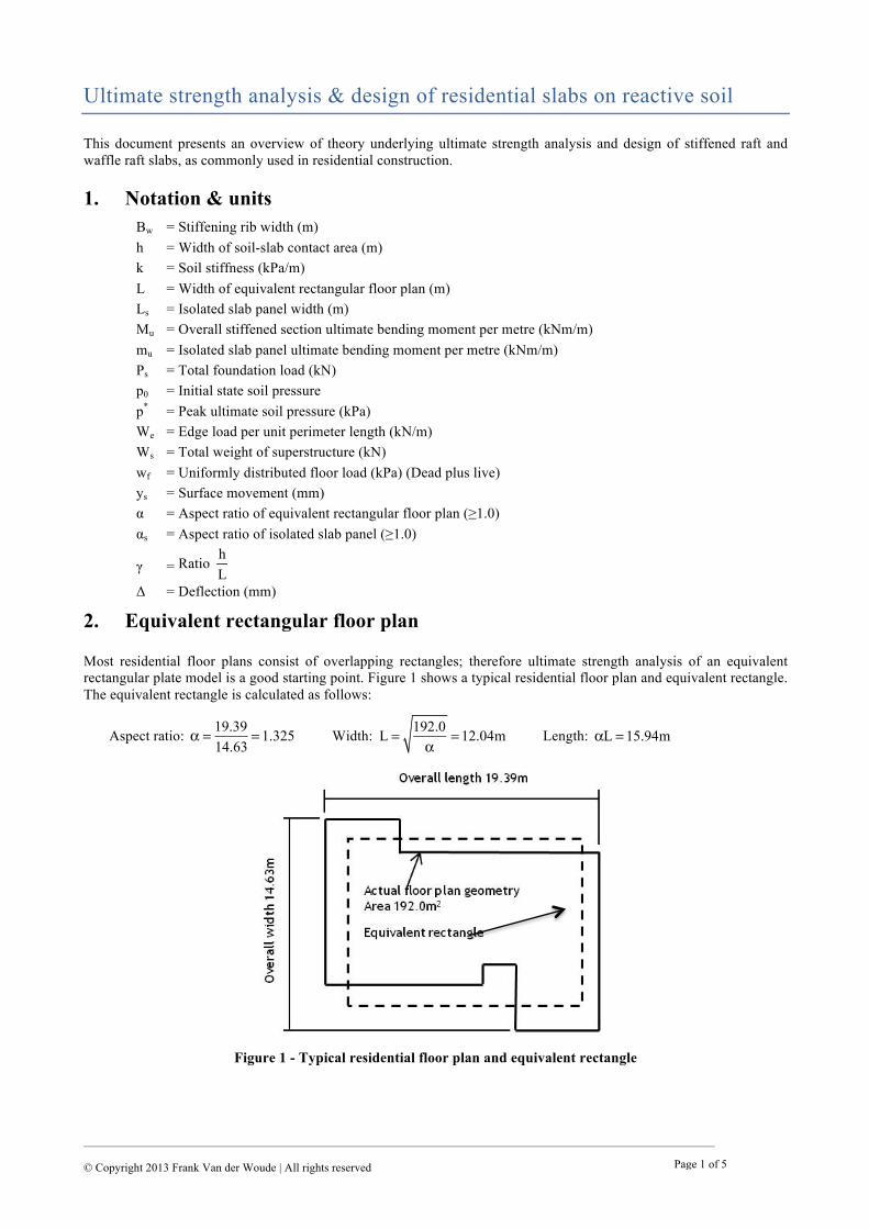
Most residential floor plans consist of overlapping rectangles; therefore ultimate strength analysis of an equivalent rectangular plate model is a good starting point. Figure 1 shows a typical residential floor plan and equivalent rectangle. The equivalent rectangle is calculated as follows:
Aspect ratio: α = 19.39
14.63= 1.325 Width:
L = 192.0
α= 12.04m Length: αL = 15.94m
Figure 1 - Typical residential floor plan and equivalent rectangle
____________________________________________________________________________________________________________ © Copyright 2013 Frank Van der Woude | All rights reserved
Page 2 of 5
3. Theory
3.1 Limit state methodology
Limit state methodology is built on identifying the governing failure mechanism and applying appropriate factors of safety and design criteria to ensure adequate in-service performance. The two major limit states in structural performance are serviceability and strength, and in the present context these two limit states are inextricably linked through soil-structure interactive performance.
The three self-evident conditions for failure of a slab are:
• Yield condition
• Equilibrium condition
• Mechanism condition
The yield line method satisfies these conditions perfectly.
3.2 Global hogging failure
3.2.1 Yield line pattern
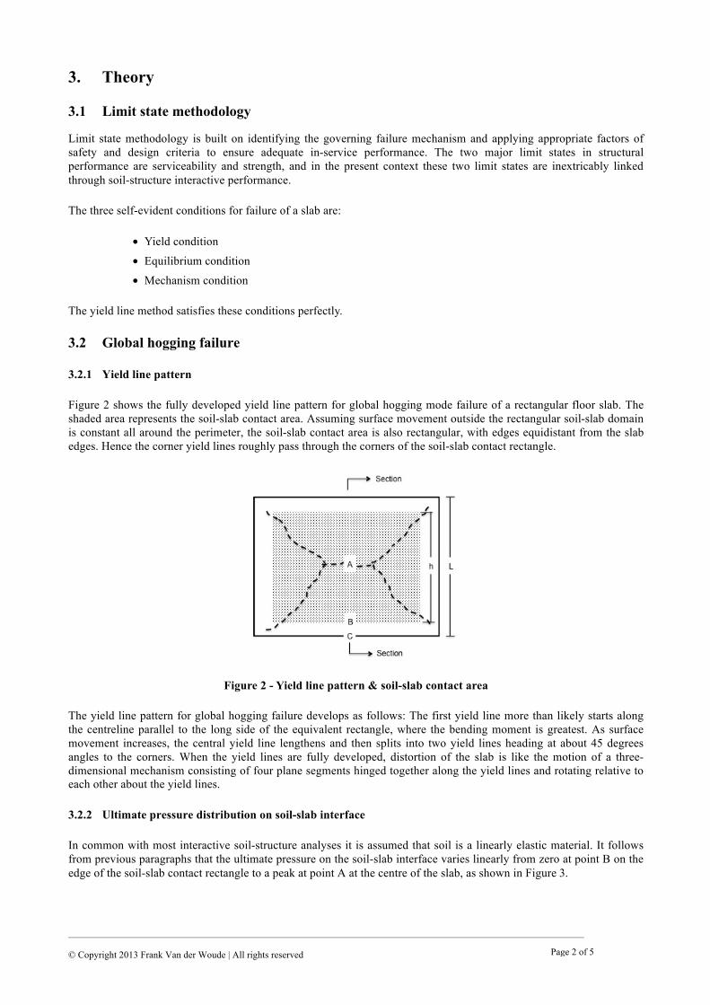
Figure 2 shows the fully developed yield line pattern for global hogging mode failure of a rectangular floor slab. The shaded area represents the soil-slab contact area. Assuming surface movement outside the rectangular soil-slab domain is constant all around the perimeter, the soil-slab contact area is also rectangular, with edges equidistant from the slab edges. Hence the corner yield lines roughly pass through the corners of the soil-slab contact rectangle.
Figure 2 - Yield line pattern & soil-slab contact area
The yield line pattern for global hogging failure develops as follows: The first yield line more than likely starts along the centreline parallel to the long side of the equivalent rectangle, where the bending moment is greatest. As surface movement increases, the central yield line lengthens and then splits into two yield lines heading at about 45 degrees
angles to the corners. When the yield lines are fully developed, distortion of the slab is like the motion of a three-dimensional mechanism consisting of four plane segments hinged together along the yield lines and rotating relative to each other about the yield lines.
3.2.2 Ultimate pressure distribution on soil-slab interface
In common with most interactive soil-structure analyses it is assumed that soil is a linearly elastic material. It follows from previous paragraphs that the ultimate pressure on the soil-slab interface varies linearly from zero at point B on the edge of the soil-slab contact rectangle to a peak at point A at the centre of the slab, as shown in Figure 3.
Limit state pressure distribution
____________________________________________________________________________________________________________ © Copyright 2013 Frank Van der Woude | All rights reserved
Page 3 of 5
Figure 3 - Ultimate pressure distribution on soil-slab interface
3.2.3 Ultimate deflection analysis
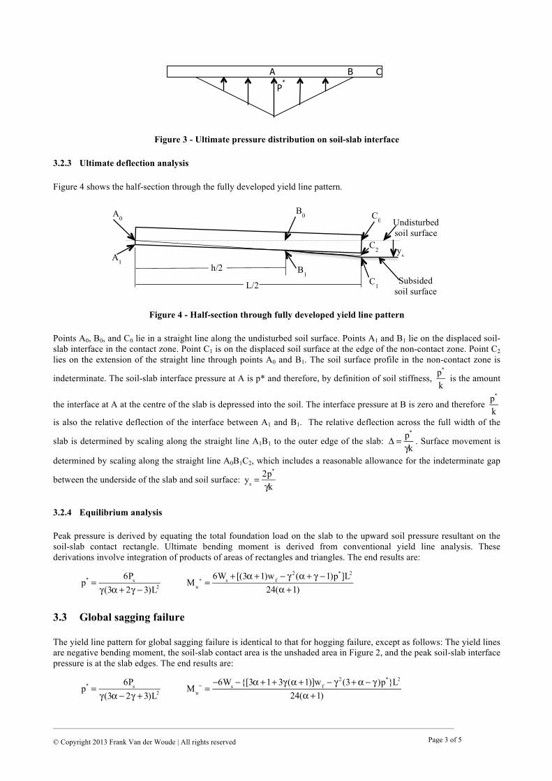
Figure 4 shows the half-section through the fully developed yield line pattern.
Figure 4 - Half-section through fully developed yield line pattern
Points A0, B0, and C0 lie in a straight line along the undisturbed soil surface. Points A1 and B1 lie on the displaced soil-slab interface in the contact zone. Point C1 is on the displaced soil surface at the edge of the non-contact zone. Point C2 lies on the extension of the straight line through points A0 and B1. The soil surface profile in the non-contact zone is
indeterminate. The soil-slab interface pressure at A is p* and therefore, by definition of soil stiffness,
p*
k is the amount
the interface at A at the centre of the slab is depressed into the soil. The interface pressure at B is zero and therefore
p*
k
is also the relative deflection of the interface between A1 and B1. The relative deflection across the full width of the
slab is determined by scaling along the straight line A1B1 to the outer edge of the slab: Δ = p*
γk. Surface movement is
determined by scaling along the straight line A0B1C2, which includes a reasonable allowance for the indeterminate gap
between the underside of the slab and soil surface: ys =
2p*
γk
3.2.4 Equilibrium analysis
Peak pressure is derived by equating the total foundation load on the slab to the upward soil pressure resultant on the soil-slab contact rectangle. Ultimate bending moment is derived from conventional yield line analysis. These derivations involve integration of products of areas of rectangles and triangles. The end results are:
p* =
6Ps
γ (3α + 2γ − 3)L2 Mu
+ =6Ws + [(3α +1)wf − γ 2(α + γ −1)p*]L2
24(α +1)
3.3 Global sagging failure
The yield line pattern for global sagging failure is identical to that for hogging failure, except as follows: The yield lines are negative bending moment, the soil-slab contact area is the unshaded area in Figure 2, and the peak soil-slab interface pressure is at the slab edges. The end results are:
p* =
6Ps
γ (3α − 2γ + 3)L2 Mu
− =−6Ws −{[3α +1+ 3γ (α +1)]wf − γ 2(3+α − γ )p*}L2
24(α +1)
P*
A
B
C
A0
ys
h/2
L/2
B0
A1 B1
C2
C0
C1
Undisturbed soil surface
Subsided soil surface

____________________________________________________________________________________________________________ © Copyright 2013 Frank Van der Woude | All rights reserved
Page 4 of 5
3.4 Local slab panel failure
The failure mechanism for isolated internal slab panels is similar to global hogging failure. The critical slab panel is at the centre of the floor plan, where the soil-slab interface pressure is greatest. Yield line analysis includes negative bending moment yield lines on the panel edges in addition to positive bending moment yield lines in the interior. The
result is: mu
+ + mu− =
(3αs −1)p*Ls2
24(αs +1)
3.5 Local corner and edge failures
Figure 5 shows the yield patterns for local corner and edge failure mechanisms. These types of failures may occur for example on a cut/fill site where the fill has not been adequately compacted around a corner or along an edge, or on a site with gilgais. The following results are obtained from straightforward equilibrium analysis:
Figure 5 - Yield lines for local corner and edge failures
Local corner failure: Mu =
Wee2
+wfe
2
12 Local edge failure:
Mu = Wee(1+ e
L)+
wfe2
2
The problem with these failure mechanisms is that there is no way of relating them to surface movement. Designers wishing to explore corner and edge failures might consider taking distance e in Figure 5 as the edge distance defined in AS-2870.
3.6 Governing failure mechanism “Like the strength of a chain is that of its weakest link…the strength of a slab is that of its weakest failure mechanism”
According to the upper/lower bound theorem in structural mechanics the governing failure mechanism for slabs on reactive soil is the one exhibiting the lowest ultimate surface movement capacity. Conversely, the governing failure mechanism is the one requiring the highest ultimate strength to sustain the most severe combination of design loading and surface movement.
It is impossible to predict a-priori which failure mechanism governs. Global hogging failure usually governs on building sites under normal soil moisture conditions at time of construction. Global sagging failure may govern on building sites that are abnormally dry at time of construction. Local corner and edge failures may govern on building sites exhibiting non-uniform soil characteristics, such as for example inadequately compacted soil on a cut-fill site, or the presence of gilgais. Local slab panel failure may govern when stiffening ribs are too widely spaced or when the slab thickness is too small, or when it supports excessive local point loads.
4. Ultimate strength performance
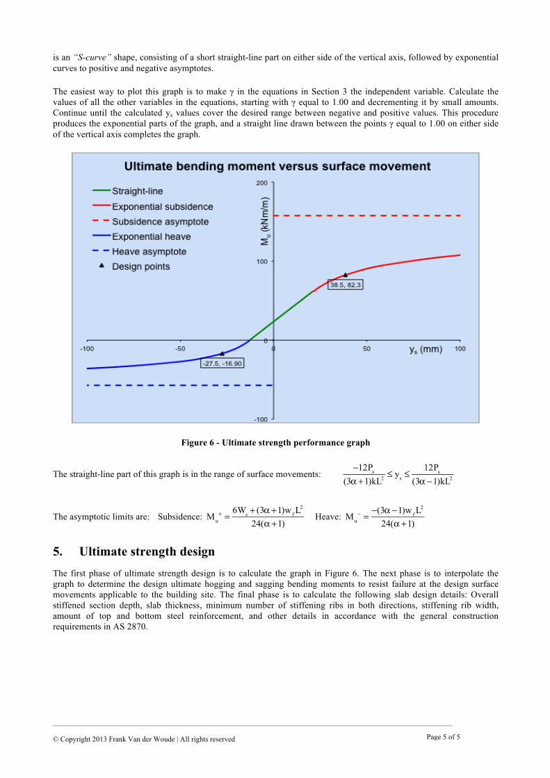
The ultimate strength performance of a stiffened slab on reactive soil is conveniently described as a function of surface movement. A typical graph of ultimate bending versus surface movement at which the slab fails is shown in Figure 6. It
e
e
e
____________________________________________________________________________________________________________ © Copyright 2013 Frank Van der Woude | All rights reserved
Page 5 of 5
is an “S-curve” shape, consisting of a short straight-line part on either side of the vertical axis, followed by exponential curves to positive and negative asymptotes.
The easiest way to plot this graph is to make γ in the equations in Section 3 the independent variable. Calculate the values of all the other variables in the equations, starting with γ equal to 1.00 and decrementing it by small amounts. Continue until the calculated ys values cover the desired range between negative and positive values. This procedure produces the exponential parts of the graph, and a straight line drawn between the points γ equal to 1.00 on either side of the vertical axis completes the graph.
Figure 6 - Ultimate strength performance graph
The straight-line part of this graph is in the range of surface movements:
−12Ps
(3α +1)kL2 ≤ ys ≤12Ps
(3α −1)kL2
The asymptotic limits are: Subsidence: Mu
+ =6Ws + (3α +1)wf L
2
24(α +1) Heave:
Mu
− =−(3α −1)wf L
2
24(α +1)
5. Ultimate strength design The first phase of ultimate strength design is to calculate the graph in Figure 6. The next phase is to interpolate the graph to determine the design ultimate hogging and sagging bending moments to resist failure at the design surface movements applicable to the building site. The final phase is to calculate the following slab design details: Overall stiffened section depth, slab thickness, minimum number of stiffening ribs in both directions, stiffening rib width, amount of top and bottom steel reinforcement, and other details in accordance with the general construction requirements in AS 2870.