Reference Manual Ultimate Equalizer Version 5, 2013, Windows 7/64bit

Bodzio Software Pty. Ltd. P.O. Box 2345 Rowville, 3178 VIC. AUSTRALIA Phone: +613-9-775-7707, Fax: +613-9-775-7708 Mail: bohdan@bodziosoftware.com.au http://www.bodziosoftware.com.au/

Bodzio Software Pty. Ltd. wishes to acknowledge, that the original version of this manual (for Ultimate Equalizer Version 3) was prepared by John Kreskovsky, of Music and Design, www.musicanddesign.com

Ultimate Equalizer DISCLAIMER.

Bodzio Software makes no warranties, either expressed or implied, with respect to the program described herein, its quality, performance, merchantability, or fitness for any particular purpose. This program is sold "AS IS". The entire risk as to its quality and performance is with the buyer. In no event will Bodzio Software be liable for direct or indirect, incidental or consequential or any other damages resulting from any defect in the program, even if it has been advised of the possibility of such damages.

CONDITIONS OF USE.

No part of this publication may be reproduced, stored in a retrieval system or transmitted in any other form or by any means, electronic, mechanical, photocopying, or otherwise without prior written permission of Bodzio Software.

WARRANTY.

Bodzio Software will replace any defective media (CD-ROM) within 28 days of receipt of any faulty media.

Warnings:

Whenever using a PC connected to your audio or home theater system, make sure the PC is powered up before turning on your amplifiers. Also, make sure the amplifiers are turned off allow then to power down before turning off the PC. This is necessary to prevent uncontrollable voltage transients, associated with PC start up and shut off, from reaching your amplifiers and speakers. Basic Requirements: The Ultimate Equalizer is very powerful software allowing DSP crossover emulation and driver response equalization to user defined acoustic targets. In order to use the software effectively you must have, as a minimum, a Windows 7 PC with 64 bit operating system, a processor speed of 2.7G Hz or greater. A Delta 1010LT sound card, a microphone for making driver SPL measurements, a microphone preamplifier, and two adapters to convert the channel 1 and 2 XLR inputs of the Delta 1010LT to RCA. With this minimum configuration you will be able to use the Ultimate Equalizer with up to 6 inputs and 8 outputs.

The output capability of the Ultimate Equalizer can be extended to 16 channels by install dual Delta 1010LT sound cards. However, such a set up will require a PC with greater processing power and speed. Please refer to Appendix F for a more detailed discussion of PC recommendations. In addition, the dual sound cards must be synchronized as discussed in Appendix G.

Table of Contents

1. Introduction 2. Menus 3. File Types 4. Working With Driver Files 5. Working With Project Files 6. Audio Measurements 7. System Design 8. Room EQ 9. Sample System Design 10. Injecting Test Tones 11. Sound card Input/Output and CAD port allocations 12. Bass Management 13. Ultimate Equalizer 19-Function Remote Control 14. Switching Inputs 15. Ultimate Equalizer in SPDIF - 96kHz/24bit all digital stereo 16. Player Mode 17. Appendix A – Why Use Fixed Point Measurement 18. Appendix B – How Does It Work? 19. Appendix C - Setting Code Preferences 20. Appendix D – Special Measurement Considerations 21. Appendix E – Sample Design Files 22. Appendix F – Sound Card and PC Sound Settings 23. Appendix G - Optimization of DSP engine 24. Appendix H - PC Recommendations

Introduction:

The Ultimate Equalizer is an advanced software tool which allows rapid and accurate development of minimum phase or linear phase crossover filters for active loudspeakers and digitally emulates these crossovers using your PC. Audio input and output is routed through suitable multi-channel sound cards installed in the PC. The Ultimate Equalizer is capable of accepting up to 8 channels of analogue input and up to 8 channels of analogue output when the PC is configured with the recommended sound card, the Delta 1010LT. Up to 16 analogue outputs can be managed if a second Delta 1010LT sound card is installed. The flexibility of the software allows the user to setup anything from a simple 2 channel stereo system, a multi-room music distribution system or a full 6 channel (5.1) home theatre system consisting of multi-way speakers. When used to design linear phase crossovers, the minimum phase associated with the woofer system high pass cut off is also linearized resulting in an active loudspeaker that has near perfect response with no time domain distortion, relative to the design point, over its entire frequency range.

Once the filter transfer functions are generated they are placed in a suitable format for emulation using long FIR digital filters. The design process consists of three fundamental phases:

1) Accurate measurement of the individual driver SPL response

2) Defining the acoustic targets for each pass-band of the multi-way loudspeaker

3) Construction the filter transfer functions which, when combined with the driver’s SPL response, produces the targeted acoustic output.

The Ultimate Equalizer includes a measurement system to obtain the required SPL data or SPL data may be imported from other measurement systems; includes a baffle diffraction simulator to model and correct the driver response for the baffle step as required; provides a library of high, low pass and equalizations functions for defining the acoustic targets; and reduces the construction of the filter transfer functions to simple drag and drop type CAD schematic generator. In addition a low frequency room equalization wizard is included.

This manual serves to describe the operation of each phase of the Ultimate Equalizer and includes an example of the design process for one channel of a simple 2-way loudspeaker. The design of additional channels follows directly.

Ultimate Equalizer V5 is recommended for i7, 960 CPUs and includes the following improvements over Version 4.

1. A tone inserted into output port selectable from a list box. This is a great feature allowing you to test and debug complex loudspeaker systems. Frequency is editable and default is 1000Hz.

2. Increased number of stored Profiles to 10.

3. Added BBM configuration screen. Excellent bass management at low

frequencies.

4. Added Summed L+R configuration for distributing stereo bass to two subwoofers.

5. UE5_MME_Lite available. It is a 2in/8out DSP, single-thread convolution

implementation, to enable it to run on older CPUs.

Menus When the Ultimate Equalizer is first opened the main menu bar is at the top of the window, as shown in Figure 1.

Figure 1. Ultimate Equalizer main menu. The main menu consists of the following selections:

1. File 2. Import/Export Data 3. Driver Files 4. System Design 5. Audio Measurements 6. User Help

Each menu item is discussed briefly below. Further explanation will be presented following the description of all menu selections. File Menu The file menu is shown in Figure 2. Each selection will first be discussed briefly and then expanded upon is required.

Figure 2. File Menu.

• New - Selecting New clears the main window and clears the code of all previously loaded data.

• Open Driver File - Selecting Open Driver file allows the user to select and load a driver file. The SPL data stored in the selected driver file is displayed in the HBT editor screen, to be discussed later.

• Save Driver File - Selecting Save Driver File saves the SPL data, which is either imported or obtained from a measurement, in a driver file with name and type defined by the user.

• Open Project - Selecting Open Project allows the user to load an existing project.

• Save Project - Selecting Save Project allows the user to save a project in the current state of design.

• Print - The Print selection will print what ever is currently displayed inside the Ultimate Equalizer main window.

• Exit - Exit closes the code. • About - Selecting About will open a small window showing the information

about the code. The window will be titled with the serial number for your installation of the code. You may need to reference this serial number when communicating with Bodzio Software.

• Preferences - Open the Preferences screen for selecting sound cards and setting plotting colors.

• Restore Defaults - Resets the preferences to those which came with the code. • C:\Folder_name\...\Driver_file_name - The driver file named will be the last

driver file which was opened. Selecting this item will reopen this file directly. • C:\Folder_name\...\Project_file_name - The project file named will be the

last project file which was opened. Selecting this item will reopen this file directly.

Import/Export Data Menu The Import/Export Data menu allows the user to import SPL data from other measurement systems and to export SPL data either from measurements made using the Ultimate Equalizer Audio Measurement tool of from driver files. The menu is shown in Figure 3.

Figure 3. Import/Export Data menu.

• Import XXX SPL [Ref = 0 dB] - Allows the user to import SPL data obtained from the XXX measurement system.

• Export SPL/Phase At 0dB - Allows the user to export SPL data for use with other software.

Driver Files Menu The Driver Files menu allows the user to edit descriptive notes saved in the driver files, access the baffle diffraction simulation tool, edit the driver SPL data and select different pen colors for plot traces. The Driver Files menu is shown in figure 4.

Figure 4. Driver Files Menu.

• Diffraction Model - Opens the baffle diffraction simulation tool. • File Editor - Opens the driver HBT Editor screens. • Pen Colors - Allows the user to change pen colors without opening the

preferences screen.

System Design The System Design menu gives the user access to a variety of default system configurations which can be used or edited as required.

Figure 5 System Design menu.

Audio Measurements The Audio Measurements menu allows the user to access the Digital – MLS measurement tool included in the Ultimate Equalizer software.

Figure 6 Audio Measurements menu. User Help User Help provides access to this Help file.

Figure 7. User Help menu.

File Types

Under the File menu two basic file types type can be accessed. These are Driver files and Project files. Driver Files Driver files contain the SPL data for the individual driver used in the construction of a loudspeaker. This data must either be measured using the measurement tools included in the Ultimate Equalizer software or imported from other measurement systems. Since speakers designed using the Ultimate Equalizer are active speakers, impedance data is not required for the drivers. There are five types of driver files which are distinguished by the file extension. These distinctions are for convenience in identifying different types of drivers.

• Woofer files - Woofer files are intended to contain SPL data for drivers used as woofers in two or more way speakers. Woofer files are named as name.wfr where name is a unique file name specified by the user when saving the driver file and the extension, wfr, is added automatically when the files is saved as a woofer file.

• Upper bass files - Upper bass files are intended to contain SPL data for drivers used as upper bass drivers in three or more way speakers. Upper bass files are named as name.uba where name is a unique file name specified by the user when saving the driver file and the extension, uba, is added automatically when the files is saved as an upper bass file.

• Midrange files - Midrange files are intended to contain SPL data for drivers

used as midrange drivers in three or more way speakers. Midrange files are named as name.mrd where name is a unique file name specified by the user when saving the driver file and the extension, mrd, is added automatically when the files is saved as a midrange file.

• Tweeter files - Tweeter files are intended to contain SPL data for drivers used as Tweeters in two or more way speakers. Midrange files are named as name.twe where name is a unique file name specified by the user when saving the driver file and the extension, twe, is added automatically when the files is saved as a tweeter file.

• Super Tweeter files - Super Tweeter files are intended to contain SPL data for drivers used as super tweeters. Super Tweeter files are named as name.stw where name is a unique file name specified by the user when saving the driver file and the extension, stw, is added automatically when the file is saved as a super tweeter file.

Project Files A Project File ultimately contains all the information about a specific project or speaker which is required to digitally emulate the crossover and play the speaker using multi-channel amplification. They are created automatically when a project is saved and can be reopened to load a previously saved project.

Working with Driver Files Drive files can be created in one of two ways:

• SPL data from another source can be imported. • SPL data can be measured using the Ultimate Equalizer Digital MLS tool and

transferred to a driver file. Creating a Driver file by Importing SPL data SPL data is imported by selecting the appropriate item from the Import/Export Data menu. For example, LMS formatted SPL data is imported by selecting the LMS SPL menu item. After making your selection an Open dialog will appear, as shown in Figure 8. The correct type files extension will automatically be selected. Search for and select the file containing the desired SPL data and click Open.

Figure 8. Open dialog for importing SPL data. After clicking Open a second dialog box will appear as shown in Figure 9.

Figure 9. Import SPL data dialog box. To import the SPL data click the Amplitude button. The data will appear in the HBT Editor, Figure 10.

Figure 10. Imported SPL data.

Reference Phase ON/OFF Measured phase response is transferred to HBT Editor Dialogue, where it can be switched ON/OFF by checkbox selection – see Figure 11 below.

Figure11. Turing OFF Reference Phase. Creating a Driver file by Measuring SPL data Please refer to the section on Audio Measurements. Saving a Driver File After the data is imported it can be saved in an appropriate driver file by selecting Save Driver File from the File menu. Select the desired file type (woofer, upper bass, ...), enter a unique name for the driver and click Save (Figure 12).

Figure 12. Save the driver file after importing SPL data.

Opening an existing driver file Driver files can be opened by selecting Open Driver File from the File menu. Upon making this selection a popup will appear, as shown in Figure 13, asking if you want to load a driver file. If there is data you wish to save before opening the driver file you should click No. Then save the data in a driver or project file as appropriate. If you are ready to proceed with loading a new driver file click Yes.

Figure 13. Open Drive File popup. After clicking Yes, a dialog box will open, as shown in Figure 14, which will allow the user to search for and select the driver file to be opened.

Figure 14. Open driver file dialog.

First, select the file type: woofer, upper bass, midrange or tweeter, and then search for the desired file. Upon selecting the driver, click Open. The driver SPL data will be displayed in the HBT editor screen, Figure 15. The function of the HBT editor will be discussed in conjunction with the Digital MLS measurement tool.

Figure 15. HBT Editor screen displaying driver SPL data.

Working with Project Files Creating a Project File Unlike previous versions of the Ultimate Equalizer, when starting a new project there is no need to load drivers into the project before hand. Drivers are loaded directly, as required, as the project is developed. Thus the creation of a project file is performed any time during project development, to save the work performed to that point. The project file is created by saving the project. Saving a Project Once a new project has been created it can be saved at any point by selecting Save Project from the file menu. When the Save dialog opens, enter a unique name for the project and click Save (Figure 16). If the project development has proceeded through the crossover design, all settings for the crossover functions will be stored in the project file. Saving previously existing projects will default to the old project name and overwrite the previously saved file unless the user specifies a new name.

Figure 16. Save Project dialog. Opening an Existing Project To open existing projects choose Open Project from the file menu. An open dialog will appear (Figure 17). Search for the project to be opened; select and click Open. Then proceed to the DSP menus to open the Ultimate Equalizer.

Figure 17. Opening an existing project.

Audio Measurements

Before you start Before you can begin to make measurements you will need to have the following equipment:

• A PC with suitable soundcard (Delta 1010LT). • A suitable microphone. • A calibration file for the microphone. • A microphone preamplifier compatible with your microphone. • A resistive probe.

When making measurements with the sound card set up correctly (see Appendix F) the output from the measurement system will appear on output channels 1 and 2 of the Delta 1010LT sound card. The input to the measurement system must be connected to input channels 1 and 2 of the Delta 1010LT sound card. If you are ambitious you can build your own microphone preamp as designed by Eric Wallin: http://mysite.verizon.net/tammie_eric/audio/preamp2/preamp2.html .This preamp is suitable for use with a Panasonic WM-60 or WM-61 mic capsule or you can purchase a microphone based on this electret condenser mic capsule. In either case the microphone should be calibrated for best results. Building the Resistive Probe The resistive probe is used to attenuate the voltage signal from your power amplifier when making measurements. Building the required probes is a simple task. To make a -10dB probe you will need one each of the following: · 47k ohm resistor · 22k ohm resistor · Female RCA jacks with plastic covers While -10dB is usually satisfactory, for different levels of attenuation different value resistors can be substituted for the 22k ohm resistor as listed in Table I. Attenuation Resistance -20 5.22k -10 22k -6 47k -3 113.5k Table I

All parts can be obtained at any Radio Shack or similar electronics parts store. Below is a picture of an RCA plug from Parts express, part #090-266.

Figure 18. RCA plug for probe construction. As shown to the left in Figure 19, remove the plastic cover from the plug and connect the 22k ohm resistor between the center terminal and the ground lug. You may wish to trim the length of the ground lug on the RCA plug. Make sure you leave enough length to solder the resistor to the trimmed lug. Then connect one end of the 47k resistor to the center lug of the plug and solder all connections. A small piece of electrical tape can be used to assure that the ground lug and center terminal do not come into contact. Replace the plastic cover. This completes the probe. The probe can be connected to the end of any interconnect cable. Connection between the test point and the probe can be made using a test lead with small alligator clips on each end, which can also be purchased at Radio Shack. It is advisable to have extra resistors for test probe construction since it is common for the resistor leads to break from flexing over time.

Figure 19. Resistor connection (left) and completed probe (right). Creating a Microphone Calibration File For the most accurate measurement of driver frequency response you should have your microphone calibrated. The calibration file should contain a list of frequency vs. amplitude (in dB) and phase. Phase response is not necessary, however, as it will be generated when the calibration data is converted for use with the Ultimate Equalizer measurement tool. The calibration data supplied with the mic should be in the form of a text file (txt extension) or an FRD file (FRD extension). This data must be processed using the Ultimate Equalizer to assure it matches the frequency scale of the Ultimate Equalizer code. To generate the calibration files for use with the Ultimate Equalizer Digital MLS tool the following procedure must be followed:

• Open the Ultimate Equalizer software. • From the Import/Export Data menu select the appropriate import format (use

IMP for FRD files, LMS for txt files).

• Search for the file containing the calibration data supplied with your microphone and open it. The microphone data should appear in the import dialog screen as shown in Figure 20.

Figure 20. Microphone data displayed in import dialog screen.

• Examine the data and if any header lines are present enter the number of lines in the header in the Erase Lines: slot at the lower left. In the example shown in Figure 20 one header line is present.

• Make sure the correct columns are checked for importing and the correct total

number of columns is entered. • If the microphone data is referenced to 0 dB enter 90 in the Scale: slot. • Click the Amplitude button. The data should appear in the HBT Editor screen

as shown in Figure 21 where the pink line is the SPL data and the green line is the phase.

Figure 21. Imported microphone data.

Phase data, if supplied with the microphone, may be suspect, depending on how the phase was determined. In the example the phase data supplied with the microphone was calculated from the amplitude using a discrete Hilbert Bode Transformation (HBT) to past 40k Hz. Due to the nature of the discrete HBT, as observed in Figure 22, the phase turns up at about 35k Hz. This is not reasonable. If the microphone response continues to drop off, the phase should continue to increase. Thus the phase must be recomputed using the HBT in the Ultimate Equalizer. This is done by tailing the amplitude data using the HBT Editor Dialog as follows:

• For the High Pass Tail enter a Stop frequency and a Slope that matches the imported data at the low frequency limit of the data.

• For the Low Pass Tail enter a Stop frequency and a Slope that matches the imported data at the high frequency limit of the imported data. However, if the calibration data extends past 24k Hz it is probable better to specify the Stop frequency as 24k Hz.

• Click the Calculate Amplitude + Phase button and observe the characteristics of the HBT result. For the example this is shown in Figure 22, where the calculated amplitude is the thin black line through the pink data line up to 24k Hz and the calculated phase is the thin blue line through the green line. Beyond 24k Hz the HBT result diverges from the imported data. Depending on the values set for the Stop frequencies and Slopes the phase may diverge from the imported data below 20 or 24k Hz. If this is the case adjust the slope as required to obtain the best phase match below and up to 24k Hz. Zero and negative values can be input for Slope is necessary.

Figure 22. HBT-generated microphone amplitude and phase response.

• When satisfied that you have obtained the best result possible click the Use As Mike Cal File button. This will automatically load the calibration data into the Digital MLS tool.

• The final calibration response can also be saved to a file by selecting Export SPL/Phase from the Import/Export Data menu.

The Digital MLS Tool The Digital MLS tool is used to make SPL measurements of the drivers to be used in your loudspeaker prior to crossover development. The MLS process uses a specific signal, called a Maximum Length Sequence, hence MLS, to stimulate the unit to be tested. This signal is digitally recorded and then mathematically transformed into the unit’s impulse response. The impulse response is then transformed into the unit’s frequency response using a Fast Fourier Transform, FFT. Before discussing how such measurements are made the controls for the MLS tool must be familiarized. The Digital MLS tool is opened by selecting it from the Audio Measurements menu.

Figure 23. Digital MLS tool screens and dialog.

When initially opened the screen should appear as shown in Figure 23. The position of the control dialog and plot screens may differ but there should be three screens: the MLS impulse Response plot screen, the MLS Frequency Domain screen and the MLS Measurements Control dialog. The MLS Measurements Control dialog has two tabs, MLS for controlling the measurement system, and Processing for performing post processing. The MLS Frequency Domain screen has three tabs, SPL + Phase where the measured SPL is displayed; Mike+Preamp where the response of the microphone calibration data can be viewed; and Post Processing where data associated with the post processing of SPL data is displayed. These screens will change automatically depending on which function is being performed. For example, when a driver is measured the screen will automatically switch to the SPL + Phase screen when SPL data is generated. Similarly, if the Post Processing tab is selected

the plot screen will switch to the Post Processing plot. The user can also switch screens at any time by selecting the desired tab. The MLS Signal Generator Control:

• MLS Length sets the length, in samples, of the MLS signal to be used in the measurement process. The lowest frequency information which can be obtained from the impulse response and the frequency resolution is set by the ratio of the Sample Rate divided by the MLS length. For example, if the Sample Rate is set to 48000 and the MLS length to 8191 the lowest frequency resolved would be 48000/(8191+1) = 5.86 Hz and the resolution would be 5.86 Hz. Resolution means that a frequency domain data point would be obtained at every 5.85 Hz.

• Sampling Rate sets the rate at which data is collected in samples per second. The Sampling Rate also sets the highest frequency at which data can be obtained. The high frequency limit is given as the Sampling Rate divided by 2. Thus a 48k Hz sampling rate yields an upper frequency limit of 24k Hz. This upper frequency limit is called the Nyquest frequency.

• Delay Read sets a time delay before data is collected from the In channel of the measurement tool. The time delay in msec is entered in the data slot to the right. The delay will be applied only if the box to the left is checked. In most cases this box should remain unchecked.

• Output level sets the audio level of the output signal. This control should be used in conjunction with your audio system volume control to set the level of the test signal. Always begin a measurement session with this level set to zero and increase it slowly to the desired level.

• Pre-emphasis is used to effectively high pass filter the test signal. It can be useful for protecting drivers from excessive low frequency stimulation. The smaller the value of pre- emphasis the higher the cut off frequency of the high pass filter. Using this feature also affects the relative SPL level of the measurement. If this feature is used the Both Channels check box should be checked and a single value of the pre-emphasis should be used for all driver measurement due to the effect on SPL level. If care is taken when performing measurements a value of zero for the pre-emphasis is satisfactory (no high pass filtering effect).

Impulse Response Processing: The Impulse Response Processing area is used to examine the impulse in greater detail and to specify the window type and length used for the FFT of the impulse response in obtaining the frequency response. An example of a 5 msec, Blackman-Harris widow is shown in Figure 24 (green trace). The window assures that the impulse response used in the FFT to obtain the frequency response goes smoothly to zero.

Figure 24. Windowed impulse response.

• Window Type controls the manor in which the impulse response is windowed. You may wish to experiment with different window types to see how they influence the frequency response.

• Window Width is used to control the extent of the window. The window width can be set by entering the length in either number of samples or time in msec. The starting point of the widow is set by placing the cursor in the plot screen where the window is supposed to start and clicking. The position can then be adjusted by using the left/right arrow keys. The Acoustical Distance from the start of the reference impulse (T = 0.0) to the start of the window will be displayed in the impulse plot screen. Placing the cursor on any blue area of the plot screen (out side the grid) and clicking will activate the arrow keys without moving the impulse to the cursor location. The Show check box controls the display of the window. When a window is used the frequency data is not valid below the frequency defined by 1/ (window length, msec). This limit is indicated by the shaded area in the frequency response plot when Show is checked.

• Zoom is used to magnify the amplitude and time scales of the impulse response. Note that the Amplitude control affects only the lower, In pulse.

• Pulse Delay is used to remove excess phase for the SPL data or to compensate for inter-channel latency. It should generally be set to zero unless inter-channel latency is observed in the loop test (to be discussed).

SPL Measurement Controls:

• Use Saved Buffer allows the user to load a previously saved impulse response for processing. When the check box is checked and the Run MLS button is clicked the user will be prompted to load the desired impulse response file.

• Show Phase shows the phase response in the frequency response plot screen when checked.

• Add xx dB to SPL is used to scale the SPL data up or down in level by the XX value entered.

• SPL Smoothing allows the user to apply smoothing the to the measured SPL data. The desired smoothing must be selected before clicking the Calculate SPL button.

• Run MLS generates the MLS signal and collects the impulse response unless the Used Saved Buffer box is checked.

• Calculate SPL performs the FFT of the windowed impulse response and displays the resulting frequency response in the MLS Frequency Domain screen under the SPL + Phase tab.

• Clear SPL clears the MLS Frequency Domain screen. • Save IR saves the impulse response for future processing. •

Linear Phase Smoothing As opposed to minimum-phase system, the phase response of a linear-phase system will appear as a flat line on the plotting screen. The lack of 360deg phase transitions, creates an opportunity to implement a better phase smoothing algorithm. Such algorithm can be activated by “checking” the “Lin-Phase” box shown below.

Figure 25. Tuning ON phase smoothing for liner-phase Calibration Files: The Calibration Files section allows the user to load (import) calibration files and select whether or not they should be applied to the frequency response measurement. Two calibration files may be loaded and are referred to as the Mike and Preamp cal files. If the calibration files were generated as discussed above they are automatically loaded when the code is opened. These calibration files will remain active until they are cleared. If no calibration data is loaded or created previously the code defaults to flat calibration response.

• Use It controls whether the calibration data is applied to a measurement. The data is applied when the box is checked.

• Import Cal. XXX File allows the user to import calibration data previously generated and saved to a file.

• Show Cal Files displays the calibration data under the Mike + Preamp plot tab screen.

• Reset Cal Files erases the calibration data and replaces it with flat calibration data.

• Export Cal Files opens a dialogue box to export calibration data.

Creating Calibration Files Microphone is inserted into the measurement chain, therefore it’s transfer function will be imprinted on the measurement results. Ideally, we should be able to derive an inverse of the microphone transfer function, which when added to measurement, would result in cancellation of the microphone transfer function. With the help of a few high-pass and low-pass filters, we could attempt to approximate microphone transfer function from the information available from manufacturer.

Figure 26. Opening dialogue for Calibration file creation. Pressing “Create Cal. Files” button will open a dialogue incorporating a selection of filters. You can also use Q-Parametric transfer function, if your microphone has sharply defined high-end roll-off.

Figure 27. Calibration file creator. Transfer function (that is SPL and phase response) will be inverted and used to correct the anticipated microphone transfer function. The Processing dialog: The SPL post processing features are accessed by selecting the Processing tab at the top of the MLS Measurements Control dialog. The Processing control is shown in Figure 36.

• At the right of the small plot screens are buttons labeled SPL>Butter X and Clear Buffer X. Clicking these button stores SPL data either from the most recent measurement or the most recently opened driver file, which ever came last. The data stored in a buffer is displayed in the small plot screen.

• The check boxes below the Show Curve column control the display of the data stored in a buffer on the main Post Processing plot screen.

• The check boxes to the left of the small plot areas allow data stored in different buffers to be summed. The + and – check boxes determine if the SPL is summed in phase or with inverted phase. Up to five different sets of data can be summed. The summation is generated by clicking the Execute Above > Master Buffer. The summation is stored in the master buffer, buffer #6. Only checked data is included in the sum.

Figure 28. Post Processing control dialogue. • Show Phase, Show Master Buffer, Show Driver controls display of the named

items in the main Post Processing plot screen. • Merge B X and B Y at Z Hz merges the SPL data in buffer X with that in buffer

Y at the Z frequency specified. Buffer X, the first buffer, must contain the data below the merge frequency and Buffer Y the data above the merge frequency.

• Add X msec delay to Buffer Y adds X msec delay to the data in buffer Y.

• Add X dB to SPL in Buffer Y increases (decreases) the SPL level of the data in buffer Y by X dB

• Add Diffraction to Buffer X superimposes the baffle diffraction response calculated in the Diffraction Model (under the Driver Files menu) on the SPL data contained in buffer X. The baffle diffraction response must be calculated previously.

• Copy Master Buffer to Buffer X copies the data stored in the master buffer to Buffer X.

Loop Testing: Before proceeding to making SPL measurements it is important to check the functionality of your sound card. This is done by performing a loop test.

Figure 29. MLS control setting for Loop Test.

• Using a Y connector, connect the line out from one channel of your sound card directly to both the left and right line inputs of the sound card.

• Open the Digital MLS tool for the Audio Measurements menu. • Set the MLS controls as shown in Figure 29. • Click the Run MLS button. • Make sure the start of the window is at T=0. The Acoustical Distance

displayed in the Impulse plot screen should be zero. • Click the Calculate SPL button. • The amplitude (red) and phase (green) response should be flat to 24k Hz as

shown in Figure 30. • If the phase response turns up or down at high frequency it is indicative of

inter-channel latency which must be corrected. If the phase turns up enter a negative value for the Pulse Delay or, if the phase turns down enter a positive value for the Pulse Delay. A value of +/- 0.01 msec is a reasonable starting point.

• Click Calculate SPL again and observe the behavior of the new phase response.

• Adjust the pulse delay until the phase is flat. This value of pulse delay should be used for all measurements made with the same sound card. The value will be saved and loaded when the UE code is started unless it is reset by the user.

Figure 30. Amplitude and phase response from correctly function sound card loop test.

Making SPL Measurements: SPL measurements taken for use with the Ultimate Equalizer should be performed in a specific manner. This will be discussed in detail in the Example Design section and in Appendix A. Please be sure to follow this procedure for the best results. This section addresses the basic use of the Digital MLS tool for making SPL measurement without the specific details of Ultimate Equalizer system design. Here the approach to far field and near field measurements is discussed as well as using the baffle diffraction simulator to correct the near field response for baffle step effects and then merging the far field and near field data. Sound Card Connections: When the sound card is set up correctly (See Appendix F) the measurement tool contained in the Ultimate Equalizer provides output on channels 1 and 2 of the Delta 1010Lt sound card. The line out from either sound card channel must be connected to the input of you preamplifier or measurement amplifier, as shown in Figure 31. The input for the measurement must is routed to inputs 1 and 2 of the Delta 1010LT. Channel 1 (left channel) of the sound card line input must be connected to the positive terminal of the amplifier used for testing using the resistive probe. Failure to use the resistive probe may result in damaging your sound card due to application of excessive voltage to the sound card line input. Channel 2 (right channel) of the sound card line input must be connected to the output of an external microphone preamplifier. Remember that the microphone preamplifier on the Delta 1010Lt sound card must be disabled (refer to sound card manual) and XLR to RCA adapters will be required to allow RCA cable connections to the channel 1 and 2 inputs. These connections are shown in Figure 31 as well.

Figure 31. Connections to and from sound card for SPL measurement. Far Field Measurement: The basic set up for far field measurements is shown in Figure 32. The microphone should be placed at the measurement distance on the design axis. If possible the measurement distance should be the intended listening distance. Accurately measure and note the distance from the tip of the microphone to the speaker baffle. This will be used as the reference distance for the measurements. See Appendix A for a discussion of the measurement setup.

Figure 32. Far field measurement setup. With all the connections made, and the speaker and microphone positioned as indicated, we are ready to make a measurement. From the Audio Measurements menu open the Digital MLS tool. Select the desired MLS length and sampling rate. Generally, an MLS length of 16383 and a sampling rate of 48000 are sufficient but increasing the MLS length to 32767 or higher is recommended for greater frequency resolution. What ever sampling rate is chosen make sure it is supported by your sound card. Remember that if you double the sampling rate you must also double the MLS length to retain the same frequency resolution. Starting with the level control at 10% and a nominal gain setting for your preamplifier (about 9:00 o’clock) gradually increase the level until an audible hiss is heard coming from the driver being tested. The hiss should be clearly audible but not so loud as to damage you speaker. Depending on the gain of you microphone preamp, the sensitivity of your sound card input, the speaker sensitivity, the measurement distance, and probe attenuation, the meters at the upper right of the MLS control dialog should appear similar to that shown in Figure 33. Your levels may vary. Make sure neither indicator is at full scale. For the highest quality measurement it is desirable to that the Ref channel level to also be one tick below maximum. This would require using a probe with different (lower) attenuation or changing the gain on your mic preamplifier, if possible. Once a satisfactory level for the IN channel is obtained the Output Level should remain constant for all driver measurements to assure the correct relative SPL levels.

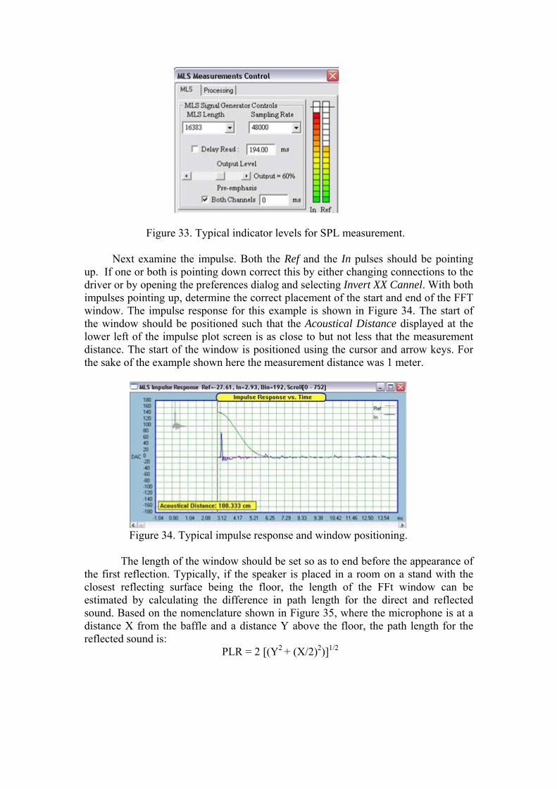
Figure 33. Typical indicator levels for SPL measurement. Next examine the impulse. Both the Ref and the In pulses should be pointing up. If one or both is pointing down correct this by either changing connections to the driver or by opening the preferences dialog and selecting Invert XX Cannel. With both impulses pointing up, determine the correct placement of the start and end of the FFT window. The impulse response for this example is shown in Figure 34. The start of the window should be positioned such that the Acoustical Distance displayed at the lower left of the impulse plot screen is as close to but not less that the measurement distance. The start of the window is positioned using the cursor and arrow keys. For the sake of the example shown here the measurement distance was 1 meter.

Figure 34. Typical impulse response and window positioning. The length of the window should be set so as to end before the appearance of the first reflection. Typically, if the speaker is placed in a room on a stand with the closest reflecting surface being the floor, the length of the FFt window can be estimated by calculating the difference in path length for the direct and reflected sound. Based on the nomenclature shown in Figure 35, where the microphone is at a distance X from the baffle and a distance Y above the floor, the path length for the reflected sound is: PLR = 2 [(Y2 + (X/2)2)]1/2

Figure 35. Computing the length of the FFT window based on the first floor reflection. The difference between the direct and reflected path length is DPL = X – PLR from which the length of the FFT window can be computed by dividing DPL by the speed of sound, 345 M/sec. For the example presented here which X = 1 M and Y = 0.92 M the window length is found to be 3.2 msec.

Figure 36. Far field SPL data for the example measurement.

Entering 3.2 msec for the window length, selecting the Blackman-Harris window and clicking the Calculate SPL button produces the frequency response as shown in Figure 36 where 1/6th octave smoothing has been selected and the SPL has been

scaled by 10dB. It should be clear that the FFT window ends before the first reflection. It should be obvious that the window length can also be set directly from inspection of the impulse response. Also shown in Figure 36 is the shading of the low frequency part of the frequency response plot below 300 Hz. This is an indication of the lower limit of the response data due to the window length. Note that 1/3.2 msec equals 312.5 Hz. Use of a longer window would extend the low frequency limit but would include the reflection in the response making the response less accurate. At this point the response can be saved in a driver file by going to the File menu and selecting Save Driver File. If it is intended to merge this response to a near field measurement the file can be opened later for use in the Processing dialog. Alternatively, the response can be stored for post processing directly by clicking the Processing tab and loading the response in one of the SPL buffers by clicking the SPL> Buffer X button, as shown in Figure 37.

Figure 37. Saving far field data in an SPL buffer for post processing. Near Field Measurement: In order to extend the response of a woofer or midrange driver to frequencies below that which limits the far field data a near field measurement is performed. This near field measurement can be corrected for the baffle step as would be present in a far field measurement and then merged with the near field data for a complete measurement of a low frequency driver. The near filed measurement is made by repositioning the microphone so that it is centered on the axis of the driver to be measured and so that the tip of the microphone lies in the plain of the baffle. Since the microphone is now much closer to the driver it is necessary to either reduce the gain on the microphone preamplifier or reduce the level of the MLS signal generated by the Digital MLS tool. An impulse response is then recorded. The FFT window must also be modified for the near field measurement. The start of the window should be placed at T = 0 so that the Acoustical Distance is zero. The length of the widow should be set to 100 msec which will place the low frequency limit of the SPL data at 10 Hz. Clicking the Calculate SPL button will then produce the near field SPL response as shown in Figure 38. As with the far field response, the near field response can be saved in a driver file. It can also be transferred to the Processing screen by selecting the Processing tab and clicking one of the SPL > Buffer buttons.

Figure 38. Near field SPL response. Symmetrical FFT Windows Linear-phase systems tend to have symmetrical impulse responses. Since conventional FFT window have clearly asymmetrical shape, it would be erroneous to apply such window to the symmetrical impulse response. UE implements 5 symmetrical window types, selected from MLS dialogue box. Symmetrical window is characterised by the start of the window (black vertical line) and the centre of the window (blue vertical line). Having completed the MLS measurement, you would scroll the Impulse Window to where the impulse response is located, and then click the left MB to the left of the impulse response location to anchor the start of the FFT window. The FFT window will appear on the screen, and then it can be moved left/right by the keyboard’s arrow keys.

Figure 39. Symmetrical FFT windows.

Example of windowed, linear-phase measurement is shown below.

Figure 40. Application of symmetrical FFT window. Please note, that the start of the window is left-shifted by the amount of time approximating the width of the window parameter. To compensate, you will need to enter a negative “Pulse Delay” parameter, close in value to window’s width.

Figure 41. Linear-phase system. Merging Far and Near Field SPL data: The complete response of a low frequency driver is a combination of the far field response and the baffle step corrected near field response, thus the near and far field SPL data must be merged and then saved in a driver file for use with the Ultimate Equalizer crossover emulator. To accomplish this, the far field and near field data must first be transferred to the Post Processing screens and dialog, and the baffle diffraction response must be previously calculated. The methods of transferring data and calculating the baffle response are discussed in separate sections which follow. Transferring SPL Data to the Post Processing Screen: There are two ways to transfer SPL data to the Post Processing area. Either the required far and near field SPL data have been previously generated and saved in separate driver files, or the SPL data will be generated as needed and directly transferred to the Post Processing screen.

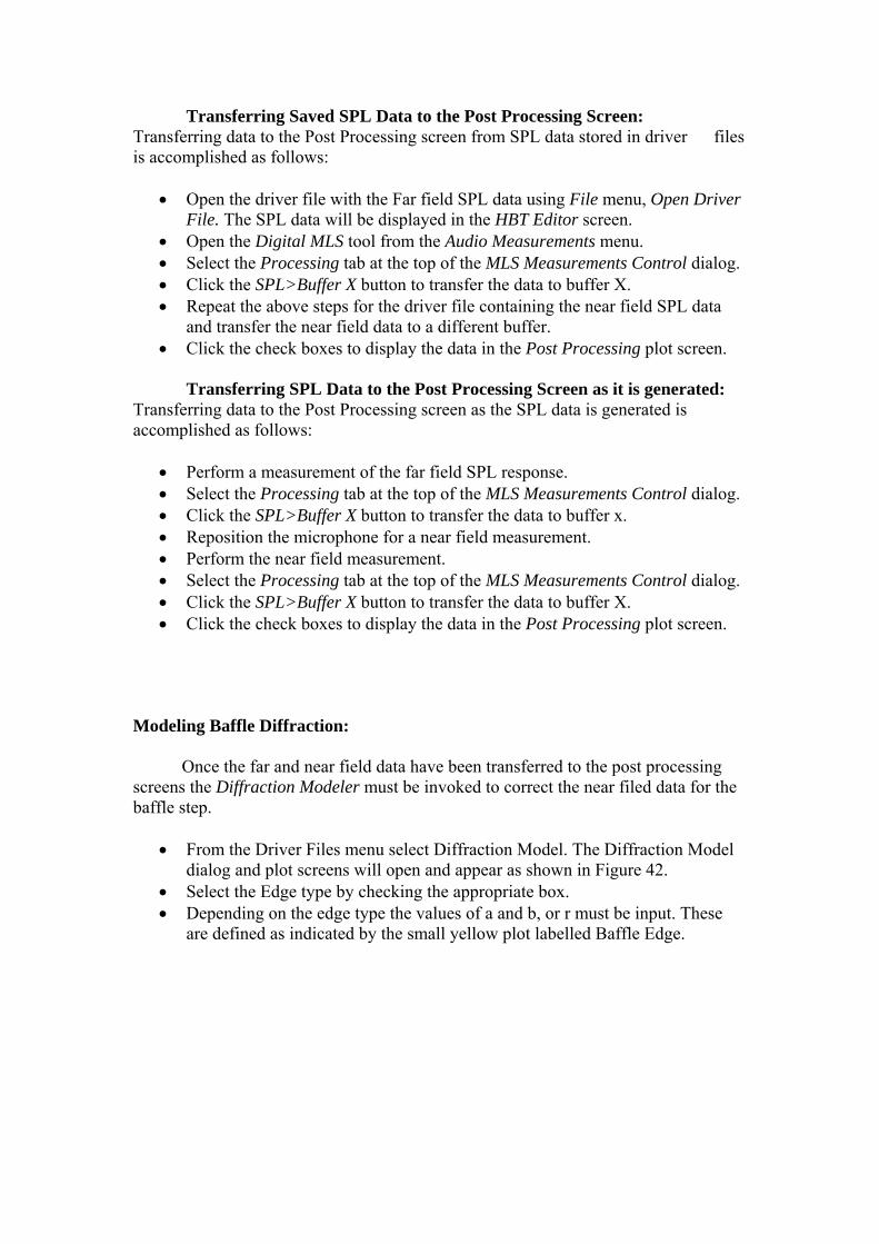
Transferring Saved SPL Data to the Post Processing Screen: Transferring data to the Post Processing screen from SPL data stored in driver files is accomplished as follows:

• Open the driver file with the Far field SPL data using File menu, Open Driver File. The SPL data will be displayed in the HBT Editor screen.

• Open the Digital MLS tool from the Audio Measurements menu. • Select the Processing tab at the top of the MLS Measurements Control dialog. • Click the SPL>Buffer X button to transfer the data to buffer X. • Repeat the above steps for the driver file containing the near field SPL data

and transfer the near field data to a different buffer. • Click the check boxes to display the data in the Post Processing plot screen.

Transferring SPL Data to the Post Processing Screen as it is generated: Transferring data to the Post Processing screen as the SPL data is generated is accomplished as follows:

• Perform a measurement of the far field SPL response. • Select the Processing tab at the top of the MLS Measurements Control dialog. • Click the SPL>Buffer X button to transfer the data to buffer x. • Reposition the microphone for a near field measurement. • Perform the near field measurement. • Select the Processing tab at the top of the MLS Measurements Control dialog. • Click the SPL>Buffer X button to transfer the data to buffer X. • Click the check boxes to display the data in the Post Processing plot screen.

Modeling Baffle Diffraction: Once the far and near field data have been transferred to the post processing screens the Diffraction Modeler must be invoked to correct the near filed data for the baffle step.

• From the Driver Files menu select Diffraction Model. The Diffraction Model dialog and plot screens will open and appear as shown in Figure 42.

• Select the Edge type by checking the appropriate box. • Depending on the edge type the values of a and b, or r must be input. These

are defined as indicated by the small yellow plot labelled Baffle Edge.

Figure 42. Diffraction Model dialog and plot screen.

• Under the Speaker-Mic Dist. + Position the check boxes control whether a directivity model is used and whether or not phase is displayed in the plot. The coordinates X and Y indicate the X, Y position of the mic.

• Under Edit Baffle Shape: Nodes the check boxes control the baffle layout.

o Add inserts a node after the last currently numbered node. o Insert after N inserts a new node between node N and node N+1. o Delete allows the user to click on a node to delete it. o Move allows the user to click on a node, driver or the mic and drag it to define the baffle size/shape and position the driver or mic. o Raster defines the distance between. The minimum raster size should be limited to 0.5 cm.

• Under Driver’s Characteristics: o Diameter defines the driver’s effective diameter.

o Location X, Y shows the position of the driver. o Dipole invokes a flat baffle dipole model. o Example 1 produces a driver on a square baffle as a starting point. o Example 2 produces only a driver as a starting point. o Piston Model controls the number of sources used to model the driver. The higher the number chosen the greater the number of sources. (Since we are generally interested in low frequency baffle step effects selecting 1 is appropriate.)

• Plot generates the diffraction response. • Done closes the Diffraction Modeler.

Once the baffle is set up clicking the plot button will generate the baffle diffraction response as shown in Figure 43.

Figure 43. Baffle diffraction response. Diffraction System Accepts Two Drivers

For dual-woofer configurations, you can now select “I have 2 drivers” option

in the Diffraction modeller – please see picture below.

Figure 44. Selecting 2 drivers for diffraction modelling.

Performing the Merge: It is assumed that SPL data has been transferred to the Post Processing screens and that the baffle diffraction response has been previously computed as described in the following sections. Figure 45 shows the Post processing screens with the far and near field response overlaid in the plot screen.

Figure 45. Far and near field data over laid in the post processing plot screen. To merge the data the following procedure is used:

• Since the near field data is saved in buffer 2, Add Diffraction to Buffer 2 is executed yielding the response shown in Figure 46. (You must uncheck and recheck the Show Curves 2 box to display the result.)

Figure 46. Diffraction added to near field response.

• Next the level of the near field SPL data must be reduced to match that of the far field using the Add X dB to SPL in Buffer Y. The far field level is the reference. This must be done with the use of judgment over a frequency range where the far and near field data have the same contour. Figure 47 shows the result of adding -17dB to Buffer 2.

Figure 47. Add -17dB to Buffer 2.

• With the SPL matched the merge can be performed at a frequency where the SPL levels are the same using Merge Buffer 2 and Buffer 1 at 500 Hz.

• To view the result, uncheck the Show Curves boxes for the buffers containing the far and near field responses and check the box to show the Master Buffer. Also check the box to view the phase. The result should appear similar to that of Figure 48.

Figure 48 Merged SPL and phase response. It is observed that the phase is not continuous at the merge frequency. This is corrected by performing an HBT (Hilbert Bode Transformation) to generate the corrected phase response. Again, the portion of the response associated with the far filed SPL is used as the reference. While the HBT can be performed in the Post Processing screens it is more convenient to use the driver HBT Editor. To do so we must first transfer the SPL data in the Master Buffer to the Driver.

• Under Copy Master Buffer to Buffer X, enter 0, for the driver buffer and click. • From the Driver Files menu open the File Editor. The display should appear

as in Figure 49.

Figure 49 Master Buffer transferred to Diver.

• Then “tail” the response: o Enter a Stop frequency and slope so as to match the low frequency roll off of the response. o Enter a Start frequency and slope so as to match the high frequency roll off of the response.

• Click Calculate Amplitude + Phase. If the phase does not match the data closely over the limits of the far field data (500 Hz to 20 K Hz in this case) you can adjust the slope of the high frequency tail and/or add delay.

o If the phase rotation is greater than that of the data, decrease the slope of the high frequency tail. o If the phase rotation is less than the data increase the slope of the high frequency tail or introduce delay and check the Include Delay in Phase box.

• If the phase does not match well at low frequency adjust the slope of the low frequency tail.

• The Include Delay in Amplitude check box will change the SPL level and should not be used.

• If during the process the plot becomes cluttered, click Refresh to clear all but the raw data.

Figure 50. HBT phase generation for merged SPL data.

• When the HBT calculation is satisfactory save the driver file by going to the File menu and selecting Save Drive File.

Differential Phase Between Drivers Due to quite simple mounting configuration on a flat, front baffle, acoustic centres of both drivers are likely to be offset against each other. This problem is explained on the diagram below, and will manifest itself during the MLS measurements as woofer phase response lagging behind tweeter’s phase response.

Figure 51. Acoustic centre difference.

Fortunately, UE allows for easy manipulation of the “location” of the acoustic centre. This is accomplished by introducing a small delay to the “forward” driver – in this case the tweeter. The amount of delay can be calculated by comparing woofer and tweeter phase responses measured with the microphone located approximately half-way between woofer and tweeter centre axis of rotation. The result is shown on the picture below.

Figure 52. Estimating phase difference between woofer and tweeter. Delay = (phase difference) *1000 /(360 x Fc) = 137 x 1000 / (360 x 2000) = 0.19msec. This value is entered in UE driver channel as the tweeter’s “Delay” parameter. There is a simpler and more accurate method to determine phase difference between two drivers. The algorithm built into the Post Processing section of MLS system allows you to calculate phase difference between two buffers: B1 and B2. In the first step, the algorithm will “unwrap” the phase response of a measured driver. The unwrapping will succeed if your phase response has clearly defined 360deg transitions – as shown on the picture below. You can help with this process by moving the start of FFT window closer to the impulse peak, and you must do this be the same amount for both measured drivers. This will ensure, that phase difference between them stays the same, regardless how much you move the start of the FFT window.

Figure 53. Identifying correct phase transitions. In the next step, you need to move tweeter SPL into Buffer 1 and woofer’s SPL into Buffer 2 – the result of this operation is shown below.

Figure 54. Transferring drivers’ data to post processing screen. Finally, nominate these buffers for differential phase response and press “Show Phase Difference” button. You may elect to “uncheck” the Show Curve boxes for both buffers, and this will clear the SPL/phase plot, leaving the differential phase plot only – see picture below.

Figure 55. Differential phase vs. frequency

System Design

When all required measurements are performed the system design can be initiated. When the Ultimate Equalizer code is initially opened the System Design CAD screen and control dialog are displayed with a default stereo 2-way layout as shown in Figure 56.

The elements of the CAD screen will be addressed separately below. Note in

Figure 56 that each channel is labelled in the lower left hand corner of the screen section containing the filter schematic for the channel. Also note that each section of the screen can be resized by placing the cursor over the vertical (or horizontal) separator and dragging.

The filter blocks are used to set the desired crossover points, type and slope,

along with system equalization or voicing and define the target SPL response for each driver and the system as a whole. Please refer to the section of Sample Design for more detailed discussion of setting the filter block parameters.

Figure 56. System Design CAD screen and control dialog. System Design Menu The System Design Menu allows the user to select several predefined sound reproduction and home theater formats. When selected, a default schematic for the chosen option will be displayed in the CAD screen and the user may proceed to edit each channel as required, setting crossover filter frequencies and slopes, equalization, loading drivers, and associating input and output nodes with the appropriate sound card channels. Blank screen options are also available to allow the user to set up his schematic from scratch.

The System Design menu is shown in Figure 57. It should be noted that some options have (Delta 101LT) listed in the selection indicating that this configuration can be emulated (played) using a single Delta 101LT sound card. Each option is described further below.

Figure 57. System Design menu options.

• Current System: The current system option allows the user to return to the presently displayed system should he move to a different part of the code. For example, if the user chooses to switch to the Audio Measurements screens he could return to the System Design screens, with the presently loaded configuration, by selecting Current System.

The following default systems have a common structure. Each channel has

two “system” filter blocks which can be used to equalize or voice the system and two “crossover” filter blocks which can be used to set the target SPL response, high pass, low pass or band pass, for the individual drivers. As discussed in the section on Schematic Editing, these default configurations can be modified by adding or deleting filter blocks as necessary.

• Stereo 2 x 2 Way: This option loads a default 2 channel stereo 2-way system as shown in Figure 47.

Figure 58. Stereo 2 x 2 way configuration.

• Stereo 2 x 3 Way: This option loads a default 2 channel stereo 3-waty system as shown in Figure 59.

Figure 59. Stereo 2 x 3 way configuration.

• Stereo 2 x 4 Way: This option loads a default 2 channel stereo 4-waty system as shown in Figure 60.

Figure 60. Stereo 2 x 4 way configuration.

• Home Theater 1: This option loads a default 5.1 Home theater system where the left and right front speakers are 2-ways and the center channel, left and right rear speakers and the subwoofer are 1-ways. The 1-way option allows the user to apply equalization to speakers used in these positions, Figure 61.

Figure 61. Home Theater 1 option.

• Home Theater 2: This option loads a 5.1 Home Theater system where all front and surround speakers are 2-ways with the addition of a subwoofer. This system requires use of multiple sound cards. Figure 62.

Figure 62. Home Theater 2 option.

• Home Theater Option 3: Similar to Option 2 but all front speakers are 3-ways. Figure 63.

Figure 63. Home Theater 3 option.

• Home Theater Option 4: Similar to Option 2 but all front and rear surround speakers are 3-ways. Figure 64.

Figure 64. Home Theater 4 option.

• Home Theater Option 5: Front left and right speakers are 4-ways, center 3-way, rear surrounds 2-ways. Figure 65.

Figure 65. Home Theater 5 option.

• Home Theater Option 6: All channels are 1-ways. This allows the Ultimate Equalizer to be used to provide only amplitude and or phase equalization of any conventional speaker with passive crossover. Figure 66.

Figure 66. Home Theater 6 option.

• Home Theater Option 7: All channels are 2-ways. This allows the user to set

up a home theater system with 2-ways front and surround speakers and dual subwoofer with different equalization applied to each subwoofer. Figure 67.

Figure 67. Home Theater 7 option.

• BLANK Stereo, Home Theater and Quadro: These options provide a blank schematic for 2, 4 or 6 channel system allowing the user to set up a filter structure to meet his special needs. The only limitation are that there can be no more than 6 sound card inputs and 16 outputs, providing such hardware capability is installed on the PC. An example for a blank Quadro is shown in Figure 68.

Figure 68. Blank Quadro CAD screen.

Control Dialog

The System Control dialog is shown in Figure 69. The control dialog serves all functions of creating, editing, plotting and playing the sound system. Beginning at the upper left are the CAD elements. These elements can be dragged and placed on the CAD screen to create a system. They consist of:

• Driver Symbol • Input node • Filter block • Connection node • Ground symbol • Room Equalization block

Directly to the right of the CAD elements are CAD controls.

• Draw: Places the CAD screen in draw mode allowing placement of symbols and connections to be made.

• Move: Allows the user to grab and move a symbol previously place on the CAD screen.

• Wipe Wire: Allows the user to “disconnect” or wipe a wire between two connected nodes by double left clicking on the wire in question.

• Wipe Component: Allows the user to delete a component, other than a wire, from the schematic by double left clicking on it.

• Show Nodes: When checked the node numbers of the connections are shown on the schematic.

• Show Raster: When checked a grid of dots are displayed on the CAD screen to aid in placement of components.

• Copy Speaker: Allows the user to copy a complete schematic from one channel to another.

• Curve Selection: Clicking Curve section opens a dialog which allows the user to select what data is to be plotted.

• Clear Plots: Clicking Clear Plots clears the plot screen. • Frequency Response Plots: Under the Frequency Response Plots heading are 6

buttons. Clicking each button plots the response of the labeled speaker channel and displays the selected response curves.

• Play Control: Checking the box in front of the number pairs allows the user to monitor the input or output level of the selected channels. Only one pair of inputs and outputs may be monitored at a time.

• Use HBT Data: When checked the HBT generated phase response is used for the drivers’ phase response as opposed to the directly measured phase. Please see the tweeter measurements for the sample design under the Far Filed Measurements section.

• SPL Only EQ: When checked the phase response of the speaker is not corrected to linear phase. When unchecked phase linearization is performed for all speakers.

• Wide Window: Setting UE to run with Wide FFT Window setting, allows for slightly more low-frequency data to be extracted from impulse response – see

picture below. This in turn, will slightly improve UE low-frequency performance.

• All 8 input ports are monitored for signal strength. Also all 16 output ports are monitored for signal strength. Orange colour is assigned to subwoofer outputs nominated from Preferences screen. Blue colour is assigned to rear speaker outputs nominated from Preferences screen.

Figure 69. Control Dialog + Instant overview of dynamic state of sound processing.

• Gain: Controls the output level from the sound card. • Play: Starts Play back of the speakers. • Stop: Stops play back.

• Del= xxx: When dual sound cards are used, calculated delay (in samples) necessary to bring the two sound cards into alignment. This number will change for every audio session triggered by the “Play” button.

• Pt= xx.xx: (Processing time) Time taken (in milliseconds) to process the active number of outputs partitioned convolution on one block of input data. This number will fluctuate slightly during the operation of the DSP engine.

• Lt= xx.xx: (Lapsed time) Elapsed time (in milliseconds) taken by WASAPI audio system to deliver consecutive blocks of audio data. This number should be close to 21.334ms. This number will fluctuate slightly during the operation of the DSP engine.

• Fr=xxxxx: Running tally of processed frames. • D1= xx.xx: Figure of merit for faster sound card. This number should be

within 4-9 units. This number will fluctuate slightly during the operation of the DSP engine.

• D2=xx.xx: Figure of merit for lagging sound card. This number should be within 6-10 units. This number will fluctuate slightly during the operation of the DSP engine. Only displayed for dual sound card installations.

If attempt to time-align the two sound cards is unsuccessful, D2=xx.xx will be replaced by the word “Synch”. In this case, simply stop and re-start the playback.

Please see Appendix G for discussion of synchronization of dual 1010LT sound cards. CAD Elements Preliminaries:

In this section the various types of filter elements and their settings are discussed. In all cases it is assumed that the various elements have been placed on the CAD screen. These elements are:

The Driver element: The Input node:

The Filter element: The Connection node:

The Ground:

The Room Equalization element:

When designing the CAD layout of each filtering system, you must apply the following rules:

• Each of these elements can be place anywhere on the CAD screen. • Each channel on the CAD screen must have one Input node. • Filter and the Room EQ elements must be placed between the Input node and

a Driver element. • The lower terminal of a Driver must be connected to a ground. • A Connection node can be placed anywhere on the CAD screen to facilitate

routing of wires.

It is emphasized that when specifying the characteristics of a filter you are specifying the target for the acoustic response of the connected driver. The Ultimate Equalizer will construct a digital filter which equalizes the measured driver SPL response to match the specified acoustic target.

To activate a specific frame of the CAD screen the user must Right Click on any open area of that frame. The channel label will turn RED indicating that frame is active for editing. See Figure 70.

To access the element for specifying the element parameters Right Click on

the yellow part of the element. For input nodes the cursor tip must be on the element. If you have problems opening the input node dialog reposition the cursor.

Figure 70. Front-Left channel label is displayed in RED indicating this channel is ready to be edited. Setting element parameters:

• Input node: Right clicking on the input node opens the dialog box shown in Figure 71. Specify the input channel of the sound card to which the input for the chosen speaker is to be connected. Multiple speakers can be connected to the same sound card input, however in doing so a warning will pop up. If multiple speakers are to be connected to the same node click OK to close the warning and continue. If the specification was in error, after clicking OK reopen the input node dialog and correct the error.

Figure 71. Input Node Dialog.

• Filter Element: The filter element is a very general element. It can serve as either a high pass or low pass filter of various order and type, a high pass or low pass shelving filter or a peak/notch filter. Referring to Figure 70, the filter blocks in the leg of the circuit connected directly to the input node should be used for system equalization or voicing. The filters connected to the drivers after the circuit branches should be used to specify the high pass and low pass SPL targets for the individual drivers. Right clicking on the yellow section opens the filter dialog as shown in Figure 72. For high pass and low pass filters the slope (6, 12, 18, 24, or 48dB/octave), cut off frequency and type, Bessel, Butterworth or Linkwitz must be specified. For voicing filters the type (Q-Parametric, Shelving +/- 6 or 12dB) and corner or center frequency must be specified, in addition to the gain and Q for the Q-parametric Peak/notch. The filter element can also be by passed by checking the by-pass box. When by-passed the filter response is omitted form the target response. In this manner filter blocks can be omitted or included in the target response without the need to delete or add elements.

If linear phase system is to be emulated the high pass and low pass filters must be of the Linkwitz type .

Figure 72. Filter and Voicing Element Dialog. Keele-Horbach Crossover This interesting new crossover approach is described in: http://www.linkwitzlab.com/Horbach-Keele%20Presentation%20Part%202%20V4.pdf

Figure 73. Keele-Horbach crossover options. UE implements: Low-pass wide, Low-pass narrow, High-pass narrow and Tweeter versions of this crossover.

• Driver Element: The driver element dialog serves several functions:

o It assigns a specific driver file and corresponding SPL data to the speaker. o It sets the frequency range over which the driver’s SPL response is to be equalized to match the target response specified using the filter elements. o It allows the addition of delay which is can be used to compensate for driver offset, if required, or to tilt the radiation pattern. o It is used to assign the sound card output channel associated with the particular driver. o It controls the phase of the output. o It controls the gain of the channel.

• It allows the response to the channel to be included or excluded in the system plots.

If you wish to determine the transfer function of a driver channel, but without the driver’s transfer function, you can clear driver’s data from this particular channel. Please press the “Clear Loaded Driver” button, and the driver’s transfer function will be cleared.

Figure 74. Driver Dialog. 1. First enter the sound card output channel number for the driver. This must be unique.

2. Click Browse and search for the driver file to be associated with this channel. An Open dialog will appear allowing the desired driver file to be selected. (Figure 75.) Then click Open to load the driver file.

Figure 75. Driver Open Dialog. 3. Set the frequency response over which the driver’s SPL response is to be equalized to match the target by specifying the low, F1, and high, F2, frequency limits. For a high pass target F1 should be somewhere below the cut off frequency and F2 in the flat band region of the response. For a low pass F2 should be somewhere above the cut off frequency and F1 should be in the flat band region. For a band pass F1 should be below the low pass cut off and F2 above the high pass cut off. A band pass target can be specified for a sealed box woofer allowing the low frequency cut off to be extended or curtailed, or to change the system Q or roll off slope. This will be discussed further in Sample Design Section. 4. Set the delay as required. Note that if SPL measurements are made in the manner suggested in Appendix A no delay or offset compensation is required for linear phase systems. The Ultimate Equalizer will compensate for the offset automatically when the suggest measurement procedure is followed. If a nonlinear phase system is the goal (no phase linearization) the delay must be adjusted to provide the correct phase tracking through the crossover region. This will be discussed further in Sample Design Section. 5. Set the correct phase for the type crossover. For linear phase crossover normal polarity should be used for all drivers. 6. Set the gain. In general this should be left at 0 dB. 7. Check or uncheck the Include in Plots box as desired.

• Room EQ element: The Room EQ element is placed between an input node and a driver element. Only one Room EQ element per speaker is allowed. It is used to equalize the low frequency response of a speaker. Please see the separate section on Room EQ.

Schematic Editing / Creating The variety of default system configurations was previously discussed in the section on the System Design Menu. Here the means of creating a custom schematic for a speaker channel will addressed along with the means of editing and coping the schematic from one channel to another.

First, from the System Design Menu select the blank format for the system to be designed. Here BLANK Stereo is selected as shown in Figure 76.

Figure 76. Selecting BLANK Stereo. Upon making the selection the System Design CAD screen will appear as shown in Figure 77.

Figure 77. BLANK Stereo CAD screen.

Click in the section of the CAD screen (Front–Left or Front-Right) to activate

the speaker to be designed. The Front-Right speaker section has been activated in this example, as indicated by the label in the lower left corner of the section turning red, see Figure 78.

Figure 78. Front-Right speaker activated.

The CAD screen is now ready to accept placement of various elements. To begin placement make sure Draw is checked as shown in Figure 78, circled in red. Elements may be selected by a left click and release on the desired element in the Design dialog. The selected component will be highlighted in turquoise. Next, move the mouse into the active section of the CAD screen. The selected element will appear as a gray outline in the CAD screen. When the element is positioned where desired left click to release the component.

Figure 79. Appearance of CAD screen after placing an input node and a filter element and a second filter element (grey outline) not yet released. .

Figure 79 shows the appearance of the CAD screen after placing an Input node and a filter element and then selecting a second filter element which has not been released yet. This process is repeated, one element at a time until all the elements required are positioned on the screen, as shown in Figure 80 for a very simply 2-ways speaker.

Figure 80. Appearance of CAD screen after placing all required elements.

After all elements are placed they must be connected by wires. These connections are made by placing the tip of the cursor on the starting connection point and using a left click/hold to drag a wire to the second connection point. When the tip of the cursor is positioned over the second connection point, release the wire. The routing of the wire depends on where the starting and ending connection points are located on the CAD screen. A wire can be dragged from either direction. If the cursor is released before the cursor is position over the second connection point the wire will disappear. Figure 81 shows the result of drawing several wires as well as a wire being dragged. Please note that the output of all elements is on the right side and the input on the left. An input element has only an output. A ground has only a single connection.

Figure 81. Connecting element by dragging wires.

If for some reason a wire must be routed around another element a connection point can be placed on the CAD screen and wires dragged to and from the connection point. See Figure 82. A connection point has no input or output.

Figure 82. Placing a connection point to route wires.

If an element is incorrectly place it can be moved by checking Move (Figure 83). Then click/hold on the element to be moved. When positioned as desired release the cursor. If wires are connected to the element they will be dragged along with the element. Only one element can be moved at a time.

Figure 83. Check Move to move and element on the CAD screen.

If a wire must be removed from the schematic due to an incorrect connection check Wipe Wire (Figure 84). Then double click on the wire to be removed. The tip of the cursor must be placed on the wire.

Figure 84. Check Wipe Wire to remove a wire from the active CAD screen.

If an element, including inputs, grounds and connection points, must be removed from the schematic, check Wipe Component (Figure 85). Then double click on the component.

Figure 85. Check Wipe Comp to remove an element from the active CAD screen.

If it is desired to display node numbers and/or the CAD screen grid check the Show Nodes and/or Show Raster. The CAD screen will appear as shown in Figure 86 when both are checked. Note that connection points connected by a wire have the same node number. Node numbers serve no purpose other than to quickly identify elements connected to each other without having to trace wires.

Figure 86. Cad screen with Node numbers and grid displayed.

After the schematic has been completed the element properties can be defined, driver SPL data loaded and the input and output ports (sound card channels) specified. Please see the section of CAD Elements for instruction on setting these parameters.

Once the CAD schematic has been completed the Copy Speaker function can be used to copy a speaker from one channel to another. The copy feature makes it easy to copy custom, multiway speaker schematics from one channel to another. Clicking Copy Speaker opens a dialog box as shown in Figure 87. Check the speaker channel to be copied and the channel the speaker is to be copied to. For this example, the Front Right channel speaker is to be copied to the Front Left channel. Clicking Done will perform the copy resulting in the CAD screen now appearing as shown in Figure 88. Note that all element settings, including the sound card channels assigned to the input and output, and the driver files associated with the original speaker, are also copied to the new channel. Thus, it is necessary to make the necessary changes to sound card input and output assignment in the Input and Driver elements. It may also

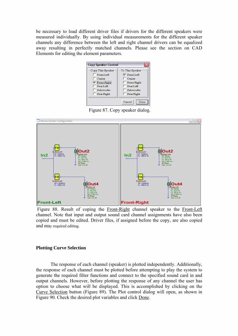
be necessary to load different driver files if drivers for the different speakers were measured individually. By using individual measurements for the different speaker channels any difference between the left and right channel drivers can be equalized away resulting in perfectly matched channels. Please see the section on CAD Elements for editing the element parameters.

Figure 87. Copy speaker dialog.

Figure 88. Result of coping the Front-Right channel speaker to the Front-Left channel. Note that input and output sound card channel assignments have also been copied and must be edited. Driver files, if assigned before the copy, are also copied and may required editing. Plotting Curve Selection The response of each channel (speaker) is plotted independently. Additionally, the response of each channel must be plotted before attempting to play the system to generate the required filter functions and connect to the specified sound card in and output channels. However, before plotting the response of any channel the user has option to choose what will be displayed. This is accomplished by clicking on the Curve Selection button (Figure 89). The Plot control dialog will open, as shown in Figure 90. Check the desired plot variables and click Done.

Figure 89. Click Curve Selection

Figure 90. Plot Control Dialog The plots which can be selected are as follows:

• Selected Filter: This is the response of the filter used as the acoustic target for the driver.

• Measured Loudspeaker Driver: The driver’s native, unfiltered response. • Inverted HBT error: This is the response of the HBT equalization required to

make the driver’s response flat over the frequency range, F1 to F2, specified in the driver dialog control.

• Inverted HBT error + Filter: This is the product of the HBT correction and the selected SPL target filter which shows the net response of the filter to be digitally emulated.

• Corrected Loudspeaker Driver: This is the response of the driver corrected by the dsp filter and which should result when the corrected driver response is acoustically measured.

• Corrected System: This displays the response of the sum of the response of all drivers which are included in the plots. When all drivers are turned on it is the response of the complete speaker system.

The phase plots correspond to the SPL plots listed above. The phase plots are turned on/off separately to keep the plot screen from being too cluttered.

Displaying Channel Response Displaying the response curves for each channel is accomplished by clicking the button for the appropriate channel in the Frequency Response Plots section of the System Control dialog, Figure 91. Each channel is plotted independently. The plot screen will automatically open or move the front if it is hidden behind the CAD screen. All channels for which speakers have been designed must be plotted to make the sound card connections before the system can be played. If you click the plot button and the message box, ”Duplicate OUTPUT Ports Found” pops up, Figure 92, click Ok and then check the input and output port assignments for all speakers.

All input and output ports must be specified for all speakers before the plots for any speaker can be displayed.

If you mistakenly click a button corresponding to a blank channel (no

components shown in that channel’s section of the CAD screen), or a channel not used for the present configuration the message popup “System Not Recognized” will appear, Figure 93. Click OK to close and click the correct plot button. To change the plots displayed, open the Plot Control dialog by clicking the Curve Selection Button.

Figure 91. Plot Control Buttons. Figure 92. Duplicate outputs warning.

Figure 93. System Not recognized popup. From time to time it may be desirable to display the response of only one, or one or two drivers in a multi-way system. Such may be the case when adjusting the delay of a driver to achieve phase alignment of a nonlinear phase system (phase correction turned off, see the SPL Only EQ check box). This is accomplished by opening the Driver symbol dialog, Figure 94, for each driver to be excluded form the plots, un-checking “Include This Port in Filter Plots” and then clicking Done.

Figure 94. Driver symbol dialog. Excluding a driver response from the frequency response plots, circled in Red; setting driver delay, circled in Blue.

The plot for a simple 2-way system is shown in Figure 95.The thin red lines indicate the specified high pass and low pass target filter responses. The green lines are the measured woofer and tweeter responses. The violet lines are the corrected woofer and tweeter response. The heavy red and blue lines are the system SPL and Phase responses (linear phase). Note that the corrected woofer response matches the target exactly between the limits of 150 Hz (F1) and 5k Hz (F2) and the corrected tweeter response matched the target between 600 Hz (F1) and 20k Hz (F2) where F1 and F2 are specified in the Drive element control dialog.

Figure 95. Plotted response of a simple 2-way speaker. Note: If the SPL measurements are performed in the manner discussed in Appendix A, driver offsets are automatically accounted for in linear phase systems. If phase linearization is turned off driver offsets must be accounted for by adjusting the delay for different drivers, as necessary. This is easily performed by selecting to plot the phase for the Corrected Loudspeaker Driver and excluding all drivers other then the two to be aligned from the plots. The delay can then be adjusted as required to visually bring the phase through the crossover region into alignment. Play Control: Before the system can be played all channels must have the input and output ports assigned and all filter and driver element properties defined (see the CAD Elements section). Before playing the following steps should be performed. Please refer to Figure 96.

• Make sure the Use HBT Data and the SPL Only EQ boxes are checked or unchecked as required (See Control Dialog).

• Check that the sample rate is set correctly: 48000 for analogue input, 44100 for SPDIF input.

• Plot each channel of the system. This assures that all the filters are correctly defined and that the input and output ports are assigned.

• Click Play to begin playback. • Adjust the volume to the desired level.

While play back is active if you are using a single Delta 1010LT sound card with 8 output channels you will see the parameter Pt, Lt, D1 and Fr displaying different numbers. This is expected. If you are using a dual Delta 1010LT setup, Del and D2 will also display numbers, if correctly synchronized. While playback is active you can monitor all input and output ports. To stop playback click Stop. When stopped the volume level will return to -42dB.

Figure 96. Play control section of the System Design Dialog. If attempt to time-align the two sound cards is unsuccessful, D2=xx.xx will be replaced by the word “Synch”. In this case, simply stop and re-start the playback. Wide Window Setting Saved to Project File Setting UE to run with Wide FFT Window setting, allows for slightly more low-frequency data to be extracted from impulse response – see picture below. This in turn, will slightly improve UE low-frequency performance.

Figure 97. Wide FFT window checked Wide FFT window un-checked

Room Equalization

High performance loudspeakers are typically described as having the first-arrival being spectrally flat within 100Hz and 10kHz in a listening room environment. Significant changes in the relative phase response are also undesirable, as this would cause changes in timbre and the clarity of pitch.

Placing a loudspeaker in a typical room will cause this sound source to excite room modes and thus influence the character of the sound. At mid and high frequencies modal density is high, as the room mods overlap, causing the room response to be more uniform and diffuse. At low frequencies, the modal density is low and mostly influenced by the axial room modes. Here, the room imprints it’s own characteristics on the sound quite profoundly.

Generally, the lower the frequency of the sound wave, the more minimum-phase characteristics will be exhibited by the room, and consequently, the use of minimum-phase room equalizer becomes more viable. But this is not the most accurate guiding criteria we should take into account, when deciding on the room optimization strategy. So firstly, it would be desirable to have some form of a “detector”, that would indicate frequency range(s) where the room is definitely exhibiting minimum-phase characteristics.

Secondly, sound waveform summation in the listening room, is a spatially dependant process, and mathematically, it involves vector addition. Therefore, we can not guarantee an equalization area within a listening room, that would be greater than ½ wavelength from the measuring point. Summation of direct and reflected sound will produce amplitude variations at the listening location that can span 40dB in magnitude. There will be frequency ranges where the summation will result in amplitude peaking (these will tend to be minimum-phase regions) and there will be frequency regions where the summation will result in amplitude dipping, or “frequency suck-outs” as some call them (these will tend to be non minimum-phase regions). However, we will also realise, that not every dip is a non minimum-phase phenomenon.

Finally, an application of a minimum-phase DSP process to control room modes, inevitably results in injecting less energy into the room within the correction frequency range. Therefore, unless the room modes are indeed loud and obnoxious, and result in significant sound discoloration, you really need to consider carefully advantages and disadvantages of room equalization. This is because low frequency active absorber will reduce the SPL at modal frequencies and will also create a perception of lacking decay at those frequencies and may become less desirable than the original modal problem in your room. It’s like - well, where has the bass gone?.

Most common approach to room acoustics would involve a careful room design, acoustic treatment, and then application of DSP to see if the outstanding problems related to minimum-phase room responses, can be reduced.

Implementation of the Room EQ When designing room equalization strategy, we are basically seeking answers to three questions: (1) what are the frequencies where we can deploy the equalizer, (2) what are the locations, where the sound is expected to be improved and (3), how much equalization we should provide.

The first step in approaching room equalization process is identification of the minimum-phase regions. A minimum-phase system is the one, that has the lowest time delay for the signals passing through it and who’s response can be inverted. If we have a system such as this, then we can create a filter, which in combination with the system, would produce a flat frequency response and correct the phase response as well. This is quite simplified view, but sufficient for our purpose. So the minimum-phase property of the room would qualify the usage of our room equalizer.

Identifying Minimum-phase regions

Let’s take a look at the measured room response. This measurement was

collected using built-in MLS system. Looking at the measured amplitude and phase responses of the loudspeaker in the room alone, it is not possible to determine the minimum-phase regions.

Figure 98. Measured SPL and phase of loudspeaker in single location.

We could anticipate, that the dips in the frequency response could possibly relate to the non minimum-phase response, but until some more convincing information confirms this, we can not be really sure at this stage.

Examining the flatness of group delay would bring us a step closer to determining the minimum-phase regions. But a better way to tackle this problem, is to look at the excess group delay. If we were able to create a system, that has the same frequency response as the measured one, but is definitely a minimum-phase type, we could then create a differential phase response by subtracting phase response of such system from the measured phase response.

Now, if the measured system was a minimum-phase type, then the excess group delay, based on differential phase response would be a flat line.

Conversely, any deviation of the excess group delay from a flat would

indicate, that this frequency range is the non minimum-phase type. Thus we have just laid down the principles of our “minimum-phase detector”.

The minimum-phase system is created by taking a Hilbert-Bode Transform

(HBT) of the measured frequency response. The HBT will output a minimum-phase phase of the measured system. We will then use this phase response in our calculations of the excess group delay.

Here is the excess group delay calculated for the measured room. We can

clearly identify two regions, where the excess group delay deviates from flat line: 55-75Hz and around 250Hz.

Figure 99. Calculated Excess Group Delay of loudspeaker in single location.

As we anticipated, these regions correspond with the dips in the measured frequency response, so now we have a confirmation of the earlier predictions. Please note, that the dip around 47Hz and many dips from 80Hz to 200Hz are not associated with the non minimum-phase behaviour of the room, and therefore could be equalized. This is where the value of the “minimum-phase detector” is becoming apparent.

However, since the above is a result of measurement in just one location, it

would now be prudent, to take advantage of the second feature of the Room EQ function, which is spatial averaging.

Spatial averaging Summation of the sound waves in the listening room is dependant on the

distance travelled by each contributing sound wave. As a consequence of this, different locations within the listening area will exhibit different frequency responses. It is not recommended to assume equalization effectiveness at more than ½ wavelength from the measurement location. For 200Hz frequency, this translates into

about 0.8 meter. Assuming typical listening room area to be 6m by 5m, the single measurement point will not be sufficient to provide efficient equalization for all sitting allocated at the back wall. You would need 3 measurements or perhaps even 4, to be on the safe side.

To illustrate this concept, two measurements have been taken in the listening

room. In both instances, the loudspeaker is an 18” subwoofer, located in a corner of the room. In the first measurement, the microphone is located near the listener’s position, close to the opposite corner of the room. The second measurement was taken with the microphone near the centre of the room. This is really not a recommended way of performing room equalization measurements. However, it illustrates rather extreme changes in the room responses and associated excess group delays.

Figure 100. Room response with microphone near the corner location.

Figure 102. Room response with microphone in the centre of the room.

Inspecting Figure 101 and Figure 102, we can conclude, that indeed, SPL and phase responses are quite different in the two locations. Also, excess group delay ( our minimum-phase detector ) shows different frequency regions for the two measurements. This is an excellent illustration of the earlier statement about sound waves summation being a position dependant phenomenon. Averaging of the two measurements produces the following graphs:

Figure 103. Averaged room response

Being guided by the excess group delay graph, we should avoid equalizing the room response around 40Hz and 170Hz.

Figure 104. Identifying minimum-phase regions. Incidentally, please note, that the blue curve on Figure 104, indicating our equalizer frequency response, is flat around the area of non minimum-phase room response. It means, that we are not doing any equalization at those frequencies, being perfectly in agreement with our earlier concerns about fallacy of indiscriminate room equalization across low-end of the frequency spectrum. So far, we have identified frequency regions and room locations, where we could apply minimum-phase equalization technique. It’s still not sufficient to execute room equalization procedure. Equalization Threshold Third and important parameter of room equalization determines how much equalization should actually be applied to the measured room response. Here, we are introducing Equalization Threshold parameter. By applying this threshold, you instruct the equalizer algorithm to design a very specific “inverse filter”. A filter, that will operate on measured SPL, but only at frequencies, where the measured SPL is above the threshold. Intuitively, we may expect, that if there was a peak in the measured SPL above the threshold level, then the equalizer would create an exactly corresponding dip in the equalizer frequency response, so the summation of the

measured SPL and equalizer frequency response would yield a flat frequency response. Lowering the Equalization Threshold into negative numbers typically results in including wider frequency bands appearing above the threshold, effectively widening the equalization frequency bands. So, this is generally desirable, however, on the downside, it also indicates, that you may need corresponding extra amplification power to restore the “0 dB”, or neutral sound level in the room. Continuing our example, let’s assume, that we have a 5dB extra amplification available. We could therefore afford to lower the threshold to -5dB (displayed as black line at 85dB). The result of this selection is shown on Figure 104 and Figure 105.

The black line on Figure 6 shows the Equalization Threshold line at 85dB ( set to -5dB by the slider control ). Sections of the measured SPL ( brown graph ) above the threshold are inverted and plotted as the room equalizer response ( blue graph ).

Combined response of room + equalizer is plotted on Figure 105 as the pink

graph. It is observable, that the curve is quite flat and sits around 85dB. To bring it to the neutral level of 90dB, you will need to insert previously mentioned amplifier of +5dB gain. As a final outcome, you have accomplished significantly smoother loudspeaker response in the room.

Figure 105. Equalization Threshold ( black curve ) set to -5dB – displayed as 85dB.

Figure 106. Setting Equalization Threshold at 0dB ( 90dB on the graph ).

In many instances, the extra amplification will not be required, as the most offending room SPL peaking is due to room modal amplification. This situation is depicted as an example on Figure 106 above. The measured room SPL between 20Hz and 54Hz is evidently above the 0dB ( or 90dB on the graph ), so you could leave Equalization Threshold at 0dB. The resulting room equalization correction is plotted as the blue graph on Figure 106.

Figure 107. Predicted room response after applying equalization to Figure 8. Now, we are ready to zoom out of the low frequency region we were focusing on, and review the Room EQ correction filter transfer function over the full UE frequency range – see Figure 108. It is observable, that phase response of the equalizer is linear and flat everywhere outside the equalization range. This is a very desirable characteristic of the phase, as it will guarantee, that no other characteristics of our sound system will be changed, except where we intend to change them. It also

proves, that our room equalizer can be operated as a minimum-phase equalizer indeed.

Figure 108. Room Equalizer’s complete Minimum-Phase transfer function.

However, the equalizer can also operate as a linear-phase device - see Figure 109. In this case, the phase response of the equalizer is a flat line and will not alter any original phase characteristics of the room response.

Figure 109. Room Equalizer’s complete Linear-Phase transfer function. Armed with the following information:

1. Identified frequencies of minimum-phase room behaviour. 2. Spatial averaged room response measurements. 3. Sensible selection of Equalization Threshold. 4. Minimum-Phase/Linear-Phase, Inverse-filter design based on 1, 2 and 3

above.

We are able to enhance the loudspeaker low-frequency performance in the listening room, across the allocated listening area. Cautionary Note On Room Equalization More extensive treatment of psychoacoustic effects associated with room equalization has been available in public domain on the internet and is obviously beyond the scope of this short paper. Nevertheless, one aspect needs to be commented upon. By applying room equalizer to the sound source (your loudspeaker) we are essentially affecting the direct-sound perception characteristics in the listening position. This could modify initial timbre of the musical note and hang as long as the note has not been contributed to by the reflected sound. We are talking here about 2ms time window for typical room. However, the amount of temporal distortion and undue nodal amplification enforced by the room, can be far more damaging to the overall listening experience. The psychoacoustic literature offers some guidance on balancing some direct sound degradation through equalization, but no definite criteria has been put forward to our knowledge. Some researchers suggest, that equalization, that results in notches deeper than -6dB should be applied with caution, as this would reduce node’s original RT60 by half. Room reverberation below 0.3s results in unusually “dead” acoustics. As always, extensive listening tests are the best criteria. Operation of the RoomEQ Controls

The “Room EQ” element is quite complex, and allows you to incorporate minimum-phase room equalization for each enclosure. This element combines up to 6 measured room SPL responses to calculate spatial average and then calculates room correction function to be applied to this particular loudspeaker. Typically, you would focus on the low-end frequency range, say below 150Hz, and apply the room correction carefully, with caution, to avoid over-equalization. The Room EQ is implemented as a drop-in element, picked from the usual list of icons on the control box. The RoomEQ control is accessible after you incorporate the “RoomEQ” element into the loudspeaker design, by placing this element on the drawing chart.

Figure 110. Room EQ Dialogue Box.

The level of automation reflects the idea of user positioning the microphone in several (up to 6 ) testing locations and just pressing one button for each location. These are the “Location X” buttons. Measurement process would require you to place the measurement microphone in Location 1, and press the button “Location 1”. Then wait for the SPL to show up. If result OK – move to Location 2 and repeat the measurement….and so on, up to Location 6. If you make a mistake – just repeat the measurement.

The rest is done by software. You may elect to run only 3 measurements, and

this will work as well. Also, if an error has been made at some location, you only needs to repeat this measurement.

Frequency range of interest is zoomed to 10-280Hz. Internally, all Room EQ

calculations are performed over the full 10-50000Hz range, it’s just the display is zoomed into the 10-280Hz frequency range. This way, calculated room correction curve can be used by the other sections of the program without the need for splicing.

Figure 111. Data displayed in the title bar. Moving the mouse cursor above the “Measured SPL/Phase” display section will display curve data on the dialogue box header see above.

The RoomEQ dialogue box has three main display sections, and the box is not adjustable. The top and bottom displays are only supporting displays. The Impulse Response (IR) Display it’s just a confirmation, the measurement was collected correctly. The Excess Group Delay is only there to identify the non minimum-phase areas on the frequency scale. All the action happens on the middle display section.

There can be one RoomEQ element per loudspeaker. So in total, there are 6 RoomEQs in 5.1 HT system possible. Each RoomEQ will operate on 6 Impulse Responses collected in 6 locations, so there is a total of 36 IRs saved to your hard disk. Managing these IRs is simple and automated as much as possible. After each measurement, the program automatically saves the IR in a dedicated file. This is a standard, 24-bit IR file as also used by SoundEasy program. Test result from Front-Left loudspeaker measured in Location 1, are saved in “Front_Left_L1.res” file and so on……Files are automatically overwritten if the measurement is repeated for the same location (without warning). The following files are created during the measurements:

Front_Left_L1.res Centre_L1.res Front_Right_L1.res Front_Left_L2.res Centre_L2.res Front_Right_L2.res Front_Left_L3.res Centre_L3.res Front_Right_L3.res Front_Left_L4.res Centre_L4.res Front_Right_L4.res Front_Left_L5.res Centre_L5.res Front_Right_L5.res Front_Left_L6.res Centre_L6.res Front_Right_L6.res Rear_Left_L1.res Subwoofer_L1.res Rear_Right_L1.res Rear_Left_L2.res Subwoofer_L2.res Rear_Right_L2.res Rear_Left_L3.res Subwoofer_L3.res Rear_Right_L3.res Rear_Left_L4.res Subwoofer_L4.res Rear_Right_L4.res Rear_Left_L5.res Subwoofer_L5.res Rear_Right_L5.res Rear_Left_L6.res Subwoofer_L6.res Rear_Right_L6.res Individual control elements function as follows:

Figure 112. Room EQ buttons.

1. Pressing “Cancel” will just close the dialogue. 2. Pressing “Done” will transfer the Room EQ +Room EQ Phase as the final

result of the room EQ process back to the Room EQ icon on the block diagram, so it becomes it’s transfer function. It will be treated as any other transfer functions in the system and will be saved to project file on HD. Next time you load the project, it will use this Room EQ transfer function.

Figure 113. Bypassing Room EQ.

3. “Bypass Room EQ” – Check this option if you need to remove the room correction curve from being included in DSP processing, without actually removing the “RoomEQ” icon from the diagram.

4. “Clear All Data” – Does exactly this – clears internal data.

5. “Scalar Average” – If checked, the averages of up to 6 measurements are

calculated as scalar quantities. If un-checked, the averages of up to 6 measurements are calculated as vector quantities.

6. “Room EQ Frequency Range” – Simply enter low- and high-end of the

frequency range you are interested in. Please do not exceed 11Hz – 275Hz frequency range.

7. “Show Measured Phase” – Enables display of measured phase.

8. “Show RoomEQ Phase” – Enables display of room correction phase.

9. “Show RoomEQ SPL” – Enables display of room correction SPL curve.

10. “Equalized Room SPL” – Enables display of room corrected SPL curve.

11. “Projected Slope Below 10Hz” it’s just the HBT tail. It will improve low-end

of the Excess Group Delay curve.

12. “EQ Amplitude Only” – If checked, this option generates flat (linear) phase response, otherwise, a standard minimum-phase response associated with room equalization curve.

13. The “EQ Threshold“ parameter (vertical slider on the left-hand side) is

adjusted in 1dB steps by the vertical slider. SPL above the threshold will be equalized by inverted HBT method. You will notice, that by manipulating the Room EQ frequency range + EQ Threshold + Location 1-6, you can influence quite well, what actually gets equalized. The idea is to have as little EQ as possible, as it all leads to user’s perception of “reduced bass”.

Figure 114. Room EQ controls.

14. “Location 1”through to “Location 6” – Works together with “Use Saved IR” check box. If “Use Saved IR” box is checked, the measurement system will load previously saved IR measurements. If “Use Saved IR” box is un-checked, the measurement system runs standard MSL test measurement sequence. You will need your hardware measurement system (microphone, pre-amp, etc…) connected and powered up to collect measurements.

15. “Volume = XX%” – Displays the output MLS signal level adjusted by the

slider below it.

16. “Window Width” – FFT window width used during MLS post-processing.

17. “Win Time [ms] - FFT window width (in milliseconds) used during MLS post-processing.

18. “Add dB to SPL” – shifts measured SPL curve up by the required number of

decibels.

19. “Add Delay [ms]” – Adds small delay (in milliseconds) to the measured IR.

20. “Ampl Zoom” – Multiplies IR amplitude by the selected factor.

21. “MLS Length” – Selects the length of MLS sequence used during the room EQ measurements.

22. “Correct With Driver On”- This option allows you to multiply unassisted

woofer’s transfer function by HBT correction curve (not the filter) developed for this driver during it’s normal equalization process. There is a list box (called “Correct With Driver On”), that allows you to select a port, that has the driver with the required HBT connected to. So for instance, you would first develop the HBT anechoic correction curve for the woofer connected to port 2. Then you can use RoomEQ MLS system to run the same woofer and include it’s correction curve in the process. Measured SPL will be modified accordingly. Now, if your HBT correction boosts the bass, this will be included in the new measured SPL, and the measured room modes will go up accordingly. Essentially, this option allows you to use RoomEQ with unassisted woofer for the development of the room correction curve, as if you actually run the UE3 with equalized driver for this purpose. You can scroll down the list box to select option “No correction” – this disables the feature.

23. “Li Ri” – Left Input and Right Input signal level indicators.

Figure 115. Room EQ MLS controls.

Making MLS Room EQ measurements Essentially, measuring room response is no different from making far-field measurements on your loudspeakers. By now, you should be familiar with this process. Please go to “Preferences” screen and select Delta1010LT Multichannel for Input Audio Device. Then select Delta1010LT Multichannel for First Output Audio Device. This will set appropriate sound card hardware for your room measurements. Next, please consult section on “Audio Measurements” and follow “Far Field Measurements” chapter, selecting up to 6 measurement locations during the measurement process. Room equalization curve should be developed with 48kHz sampling frequency and long MLS sequences. Please select 262143 length for the MLS sequence.

Sample System Design

In this section an example of the Ultimate Equalizer applied to the design of a simple stereo 2-way speaker system will be presented. The example design will be for a small two way speaker with 5” woofer and 1” dome tweeter.

It is assumed that the speaker enclosure has been designed and the drivers are mounted on the baffle. Since details of the functionality and use of the various features of the Ultimate Equalizer software have been addressed in other sections of this manual the sample design will focus on the design of a single channel. Designing more complex systems follow directly.

The design procedure follows this outline:

• Obtain and save near field measurement of any drivers requiring near field, far field merging.

• Obtain and save far field measurements for all drivers with the microphone at a fixed position representative of the design position. If merging to near field data is not required an HBT using the File Editor is performed before saving.

• For each driver requiring merging of the near and far field data, sequentially: o Load the far and near filed data into the Digital MLS Post Processing tool. o Model the baffle diffraction. o Correct the near field data for the baffle step. o Merge the corrected near field and far field data. o Perform an HBT of the merged data using the File Editor and save.

• After the driver files have been created and saved select the appropriate CAD layout for the system design.

• If necessary, layout the required schematic for the first channel to be designed. • Set the various filter parameters as required. • Load the required drivers and set the parameter for driver equalization. • Specify the input and output ports and plot the system.

Near Field Measurements: With microphone centered on the woofer axis and the tip of the microphone in the plane of the baffle the near filed SPL data of the woofer is obtained using the Digital MLS tool opened from the Audio Measurements menu. A sufficiently long FFT window must be specified to assure accurate low frequency data. The window should start at T = 0 for the impulse response (Acoustically distance = 0.0). The measurement for the sample design is shown in Figure 116. After obtaining the SPL data, the near field response is immediately saved in a woofer driver file with unique name by selecting Save Driver File from the File menu.

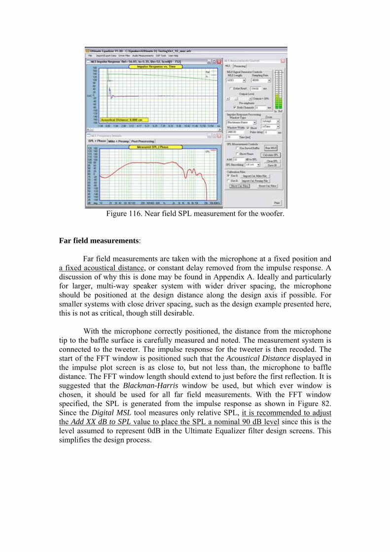
Figure 116. Near field SPL measurement for the woofer. Far field measurements: Far field measurements are taken with the microphone at a fixed position and a fixed acoustical distance, or constant delay removed from the impulse response. A discussion of why this is done may be found in Appendix A. Ideally and particularly for larger, multi-way speaker system with wider driver spacing, the microphone should be positioned at the design distance along the design axis if possible. For smaller systems with close driver spacing, such as the design example presented here, this is not as critical, though still desirable. With the microphone correctly positioned, the distance from the microphone tip to the baffle surface is carefully measured and noted. The measurement system is connected to the tweeter. The impulse response for the tweeter is then recoded. The start of the FFT window is positioned such that the Acoustical Distance displayed in the impulse plot screen is as close to, but not less than, the microphone to baffle distance. The FFT window length should extend to just before the first reflection. It is suggested that the Blackman-Harris window be used, but which ever window is chosen, it should be used for all far field measurements. With the FFT window specified, the SPL is generated from the impulse response as shown in Figure 82. Since the Digital MSL tool measures only relative SPL, it is recommended to adjust the Add XX dB to SPL value to place the SPL a nominal 90 dB level since this is the level assumed to represent 0dB in the Ultimate Equalizer filter design screens. This simplifies the design process.

Figure 117. Tweeter far field SPL measurement. The File Editor is opened from the Driver Files menu and an HBT performed as shown in Figure 118. Use the Include Distance in Phase option to obtain the best phase match at high frequency. If necessary, the slope of the high frequency tail can also be adjusted to obtain a good phase match. The slope of the tail need not match the apparent slope of the SPL data. It is more important to match the phase. Then the data is saved in a tweeter (.twe extension) driver file with unique name.

Figure 118. HBT applied to the Tweeter response. The measurement system is reconnected to the woofer and the woofer far field impulse recorded. The far field SPL response of the woofer (and any other drivers) is then generated without making any changes to MLS tool settings including the Output level, MLS length, sampling rate, FFT window or the Add xx dB to SPL. This will assure that the relative SPL data is consentient for all drivers. The Acoustical Distance and FFT window length should remain exactly as used for the tweeter. The result is shown in Figure 119. Since the sample design is a simple 2-way speaker the woofer

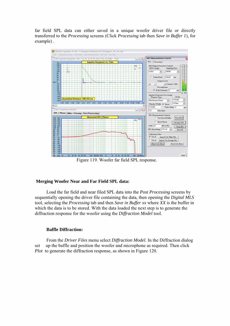
far field SPL data can either saved in a unique woofer driver file or directly transferred to the Processing screens (Click Processing tab then Save in Buffer 1), for example) .

Figure 119. Woofer far field SPL response. Merging Woofer Near and Far Field SPL data: Load the far field and near filed SPL data into the Post Processing screens by sequentially opening the driver file containing the data, then opening the Digital MLS tool, selecting the Processing tab and then Save in Buffer xx where XX is the buffer in which the data is to be stored. With the data loaded the next step is to generate the diffraction response for the woofer using the Diffraction Model tool. Baffle Diffraction: From the Driver Files menu select Diffraction Model. In the Diffraction dialog set up the baffle and position the woofer and microphone as required. Then click Plot to generate the diffraction response, as shown in Figure 120.

Figure 120. Modeling of baffle diffraction for woofer.

With the diffraction modeling completed, return to the Digital MLS tool and, as discussed in the manual section on Merging Far and Near Field SPL data: Add diffraction to the buffer containing the near field data.

• Add xx dB to the near field data so as to match the far field SPL level at the selected merge frequency.

• Merge XX to YY, where XX is the buffer for the far field data and YY is the buffer for the near field data. The result should appear as indicated in Figure 86.

• Copy Master Buffer to buffer 0 (copy to driver). • From the Driver File menu select the File Editor and perform an HBT on the

merged response. • Save the response in a woofer (wfr extension) driver file.

Figure 121. Merged near and far field woofer SPL data.

Figure 122. HBT applied to the merged Woofer response. Designing the Crossover: Once the SPL data for all the drivers to be used in the system have been measured and driver files saved you are ready to design the crossover for each channel. In this sample for a stereo 2-way system one channel of the system will be designed. The second channel with be generated by copying the first channel to the second. Initially a linear phase system will be designed. It will then be show how to proceed to make the system nonlinear phase, as a typical passive speaker would be. Linear Phase system:

• From the main menu select System Design and choose the configuration best suited for your system. Since a stereo 2-way system is being designed the available choices are either Stereo 2 x 2 Way or BLANK Stereo. Here the Stereo 2 x 2 way is chosen which eliminates the need to manually layout the speaker schematic in the CAD screen.

Figure 123. Choose the configuration for the speaker system form the System Design menu.

• The CAD screen will appear as shown in Figure 124. The default configuration for the stereo 2 x 2 way speaker consists, for each speaker, an input, then two filter elements which can be used for voicing the speaker, then two filter elements for each driver to set the acoustic targets for the high pass (tweeter) and low pass (woofer) bands. The input and output ports will be set to default values, shown in large green (input) and red (output) type by the input and driver elements, and may be changed if desired.

Figure 124. Cad screen appearance after selecting the Stereo 2 x 2 way configuration.

• In the System Design Control dialog it is recommended that the Use HBT Data box be checked, Figure 125, provided that the HBT phase was generated before saving the driver files. The SPL Only EQ box is unchecked which will result in linear phase speakers.

Figure 125. Check the Use HBT Data if the HBT phase was generated before saving the driver files.

• Right click on any area of the CAD screen for the channel you which to design. The channel label in the lower left hand corner of the selected channel will turn red indicating that speaker is ready for editing, Figure 126.

Figure 126. Front-Left shown in RED indicating the front left speaker channel is ready for editing.

• We are now ready to edit the parameters of the filter elements and drivers associated with the left front speaker.

• Initially the voicing elements will be bypassed. This is accomplished by opening each element and checking Bypass The Element, Figure 127.

Figure 127. Bypassing an element.

• The bypassed elements will be labeled as such in the CAD screen, Figure 128.

Figure 128. Bypassed voicing elements. By-passing Components and Plots It is very handy to be able to switch ON/OFF a transfer function of a complete filtering block. By doing so, you effectively by-pass this component. You can do this on any active screen section by double-clicking the left MB over this filter. You will see, that filter’s parameter’s data will be replaced by “By-Passed” tag. Similarly, if the SPL plotting screen is too clogged, you can turn ON/OFF plots for any channel by double-clicking the left MB over this loudspeaker icon. You will see, that “OK to Plot” will be replaced by “Don NOT Plot” tag – see below.

Figure 129. By-pass and “Do NOT Plot”.

• Next the crossover frequency, type and order are set for the woofer and tweeter. For this linear phase example a 2k Hz, Linkwitz/Riley 4th order crossover is to be used. Please note that to insure flat response only Linkwitz/Riley crossover can be used for linear phase systems.

• To set up the crossover choose the circuit branch which will be associated with the tweeter, open one of the filter block (right click on the element) and set the filter configuration, filter type and cut off frequency, Figure 130. The click Done. This will set the high pass target for the tweeter. As with the bypassed voicing elements, the filter configuration will be shown on the CAD screen.

Figure 130. Setting the tweeter high pass target.

• In a similar manner, choose a filter element in the branch which will be associated with the woofer and set the element parameters for the woofer Linkwitz/Riley, 4th order,, 2k Hz, low pass target, Figure 131.

Figure 131. Setting the woofer low pass target.

• For the moment the remaining filter blocks in the woofer and tweeter branch will be bypassed as was done for the voicing elements. Thus, the front left channel CAD screen will appear as shown in Figure 132 when this is done.

Figure 132. Cad screen appearance after setting the woofer and tweeter targets and bypassing remaining components.

• We can now load the driver’s SPL data into the driver element. Starting with the tweeter, right click on the driver element in the tweeter branch to open the element dialog, Figure 133.

Figure 133. Load the tweeter file and set the necessary parameters.

• Click Browse and load the tweeter. At this time also set the frequency limits, F1 and F2, for the HBT equalization of the tweeter response. The equalization should begin somewhere below the crossover frequency and end above it. Here 500 Hz and 20 K Hz have been chosen for the HBT limits. This means that the tweeter SPL response will be equalized to match the target filter response exactly between those limits. Also check Include This Port in Filter Plots. Then click Done.

• Perform the same operation for the woofer. Set the limits for the HBT equalization so the F1 is below the crossover point and F2 is above it. For this example F1 = 200 Hz and F2 = 5k Hz have been initially chosen Figure 134. These may have to be adjusted after viewing the response plots.

Figure 134. Load the woofer file and set the necessary parameters.

• We now have the basics of a completed 2-ways speaker and can plot the response. Initially it is helpful to plot only the selected filter responses and the measure SPL of each driver. (For 3 or 4 way system you may which to start by plotting only the woofer to keep the plot screen less cluttered).

• Open the Plot Control dialog by clicking the Curve Selection button and check Selected Filter and Measured Loudspeaker Driver, Figure 135. Then click Done.

Figure 135. Plot Control Dialog.

• Next click the button to plot the Front Left Speaker, Figure 136.

Figure 136. Click Front Left generate plots for the left front speaker.

• The selected response plots will appear the plot screen as shown in Figure 137.

Figure 137. Plots of the selected high pass and low pass filter targets and driver SPL response.

• In Figure 137 notice the red circle. In this design we are not attempting to alter the low frequency response of the woofer. Thus it is advantageous to have the lower frequency limit for the HBT equalization of the woofer set to the frequency where the target response crosses the measured SPL data. This is at about 220 Hz.

• Open the woofer and set F1 to 220 Hz. • Click the Curve Selection button and now add select Corrected Loudspeaker

Driver to the curves to be plotted. • Clear the plots and re-plot the response for the Front Left speaker. The result

for the example is shown in Figure 138. Notice how the corrected Loudspeaker Driver response of the woofer follows the measured SPL data below the woofer F1 frequency of 220 Hz. Also notice that both the woofer and tweeter correct response, shown in violet match the target filter curves exactly between the limits of F1 and F2 (220Hz and 5k Hz for the woofer, 500 Hz and 20k Hz for the tweeter).

Figure 138. Plots of the selected high pass and low pass filter targets, driver SPL and corrected driver responses after changing the woofer F1 frequency.

• An example of a poorly selected woofer F1 is shown in Figure 102 where F1 = 60 Hz. This is not advisable.

Figure 139. Poorly selected woofer lower HBT frequency, F1. Note the abrupt change in slope at 60 Hz.

• The final system frequency response is shown in Figure 140 with the correct woofer F1, and where the curves to be plotted were set to the Selected Filter, the Corrected Loudspeaker Driver, and the Corrected System SPL and phase. The system SPL is shown as the thick red line and the system phase by the thick green line. As can be seen, since the driver were measured using the single position method discussed in Appendix A, the Ultimate Equalizer automatically correct for the driver offset resulting in flat response through the crossover.

Figure 140. Final system frequency and phase response.

• With the system now designed we can move on to the Right front speaker. Since this example is a simple stereo system this is easily accomplished by opening the Copy Speaker control from the System Design control dialog, Figure 141.

Figure 141. Copy Speaker and Copy Speaker Control dialog.

• After performing the copy Right Front speaker will have identical settings, including the input and output port assignments and drivers, Figure 142.

Figure 142 Appearance of CAD screen after copying the Front Left speaker to the Right Front.

Note input and output port assignments are the same which results in a conflict.

• Before the system can be played or additional plots produced it is necessary to resolve the conflict between left and right input and output port assignments.

• Open the right speaker input element and assign the correct port number to the right speaker.

• Open the right speaker driver elements and enter the correct output port numbers.

• If separate SPL measurements were made for the driver using in the left and right speakers the correct driver files for the right speakers should be loaded at this point.

• Once all the corrections have been performed all the channels of the system must be plotted to make the connections to the sound card and define the filter functions. After plotting all channels the system is ready to be played.

Changing the Voicing of the System: The voicing of each speaker can be change from flat by setting the parameters of the voicing elements, Figure 143. This is accomplished by opening the filter element to be used,

Figure 143. Voicing elements. setting the parameters as desired and making sure the element is not bypassed. The default speaker configuration include 2 voicing element for each speaker channel. Additional voicing elements can be added, if required, by editing the schematic. This requires wiping a wire in the input branch of the circuit, moving other elements, as required, to make space for the additional voicing element(s), and reconnecting the elements. Alternatively, additional elements can be placed elsewhere on the CAD screen and then connected using the connection element to route the wires, as shown in Figure 144.

Figure 144. Using connection elements to route wire to added voicing elements. There are a number of filter functions which can be used for voicing including: Q-Parametric peak/notch filter Shelving -6dB (1st order low pass shelf) Shelving -12 dB (2nd order low pass shelf) Shelving +6dB (1st order high pass shelf) Shelving +12dB (2nd order high pass shelf)

The parameters to be ser for each function are the center frequency, the gain (positive or negative), and for the Q-parametric the filter Q. An example of the effect of adding a low pass shelf with 4dB gain and center frequency of 200 Hz to boost bass, and a Q-parametric notch with center frequency of 3k Hz, Q = 1 and -3dB gain (a “BBC dip”) is shown in Figure 145. The response should be compared to that shown in Linear Phase System.

Figure 145. Effect of low pass shelf bass boost and Q-parametric BBC dip voicing elements on the system response. Extending/Targeting Bass Response Targeting Bass response The design of the sample 2-way system was implemented using only a high pass and low pass filter for the crossover. This required that the low frequency specification of the equalization range, F1, for the woofer, be carefully chosen to avoid a sharp discontinuity in the low frequency roll off of the woofer. (See the discussion in the Linear Phase System section.) However, there is another way to assure the response rolls off as desired or to alter the roll off. This is accomplished by adding a high pass filter response to the woofer target which matches the intended box alignment as closely as possible and setting the lower equalization frequency range, F1, to a frequency below the corner frequency of the high pass target. In the sample design. For the sample design this is accomplished by specifying the previously bypassed filer element in the woofer branch of the circuit as a 2nd order Linkwitz high pass filter with corner frequency (90 Hz) chosen so as the target response best matches the box alignment as shown in Figures 146 and 147. The woofer equalization range was specified as 20 Hz. The resulting system response is shown in Figure 148.

Figure 146. High pass filter element introduced in woofer branch to target the enclosure low frequency alignment.

Figure 147. Plotted woofer measured response and woofer target response with added high pass filter element.

Figure 148. System frequency response with woofer response equalized between 20 and 5k Hz to match the specified 2nd order, 90 Hz high pass, 4th order, 2k Hz low pass target.

Note that below the value specified for the woofer F1 the system response rolls off at approximately 4th order. This is because below F1 the targeted filter response is superimposed on the raw woofer SPL response. The 2nd order roll off of the woofer combined with the 2nd order roll off of the target yields a 4th order roll off below F1. Extending Bass Response The same technique used to control and match the woofer response to the box natural alignment can also be used to extend the bass response of a sealed enclosure. As an example, suppose that it was desired to change the woofer roll off form the natural box alignment ( 2nd order, 90 Hz, Linkwitz high pass) to a 2nd order, 60 Hz Butterworth. This can easily be accomplished by changing the parameter of the high pass element in the woofer circuit to the desired response. The result of such a specification is shown in Figure 149. Noted that by extending the low frequency cut off, significant boost must be applied at the lower frequencies. Thus, care should be taken when extending the bass response. Approximated 12dB boost will be added to extend the response of a 2nd order roll off by 1 octave.

Additionally, while the same procedure can be used correct the alignment of a ported system, for example from a Butterworth to a Linkwitz response, the cornet frequency of a ported system should not be extended below the port tuning frequency. Such an extension would result in extreme excursion of the woofer and possible damage.

Figure 149. System response with woofer high pass target set to a 2nd order, 60 Hz Butterworth response. Non-Linear Phase System A non-linear phase system is a speaker for which the phase linearization performed by the Ultimate Equalizer is not applied. The result is a speaker which has the same phase response that a similar speaker with passive or active analog crossover would have. The design process is identical to that of the linear phase system with one exception; the effect of driver offset must be accounted for in the design. This is

straight forward when using the Ultimate Equalizer and the discussion will pick up form the completed linear phase design. The response of the completed linear phase system is shown in Figure 150. The heavy red and green traces show the system amplitude and (linear) phase. The violet traced show the corrected amplitude response of the drivers and the orange traces show the phase response of the individual drivers before the system phase is linearized.

Figure 150. Responses of linear phase system and corrected drivers.

The crossover is a 2k Hz, 4th order Linkwitz type. Recall that when linear

phase systems are designed Linkwitz type crossover must be used. Note that the phase of the drivers is not aligned through the crossover region. This system is easily converted to a non-linear phase system by making a single change in the System Control Dialog. This change is to check SPL Only EQ as shown in Figure 151.

Figure 151. Check SPL Only Eq to make the system non-linear phase. Re-plotting the system response with SPL Only EQ checked results in the response shown in Figure 151. Note that the system phase (green) now shows the typical rotation of a convention speaker system and that there is a dip in the response in the crossover region. This dip is due to the uncompensated driver offset and resulting phase misalignment. Also note that the system phase follows the woofer phase at low frequency and the tweeter phase at high frequency.

Figure 151. Response of non-linear phase system. The driver off set must be compensated for to correct the response dip in the crossover region. Since this is a Linkwitz type crossover the phase difference between the woofer and tweeter should be zero at the crossover point. Examining the phase of the individual drivers it can be determined that the woofer phase is about 90 degrees at the crossover frequency. The tweeter phase at the crossover point is about 170 degrees. Thus the phase difference is 80 degrees at 2k Hz. Form this the delay, in msec, required to correct for the offset can be computed directly: Delay = (phase difference) *1000 /(360 x Fc) = 80 x 1000 / (360 x 2000) = 0.111 msec. The question is then, which driver should the delay be applied to? Looking at Figure 151 again, it is apparent that at low frequency the system (and woofer) phase trace is below that of the tweeter. The woofer phase reaches -180 at about 1.4K Hz. The tweeter phase reaches -180 degrees at about 1.9 Hz. Thus the woofer phase is “rotating” faster than that of the tweeter indicating that the woofer is delayed more than the tweeter. (This may appear obvious for this simple 2-ways speaker, but in multiway system the situation may be more complex.) Since the woofer shows greater delay, the delay required to correct for the offset, as computed above, must be applied to the tweeter. Open the tweeter element control dialog and enter the delay (in msec) in the Channel Delay slot (circled in RED) and click done.

Figure 152. Enter the computed delay in the tweeter control box.

Re-plotting the system response shows that the response, Figure 153, is now flat through the crossover region and that the phase of the woofer and tweeter over lay each other through the crossover region, as they should for Linkwitz type crossover. If the response is not flat, make sure the delay was added to the appropriate driver. Additionally, it may be necessary to make fine adjustment to the delay depending on how accurately the phase curves were read. Also remember that is the crossover is of the 2nd order Linkwitz type one driver, typically the tweeter, must be set to reversed phase in the driver dialog before the phase difference through the crossover region is determine. (Note that linear phase 2nd order Linkwitz crossover should have all drivers connected with normal polarity.)

Figure 153. System response with delay compensation for driver offset. Finally, the offset compensation can be further checked for Linkwitz type crossovers by inverting the polarity of one of the driver from that which it would normally be. A deep notch at the crossover frequency should be observed. Figure 154 shows the response for the sample system with the tweeter polarity inverted.

Figure 154. System response when the tweeter is connected with inverted polarity.

Playing the System Warning: When ever using the Ultimate Equalizer in an audio or home theater system, make sure the PC is powered up before turning on the amplifiers. Also, make sure the amplifiers are turned off and allow then to power down before turning off the PC. This is necessary to prevent voltage transients associated with PC start up and shut off from reaching you amplifier and speakers. Whether the design is a linear phase or nonlinear phase system, at this point the system is ready for play back. Play control is further discussed in a separate section. Make sure the correct sound card is chosen for play back from the Preferences screen. Connect the sound card input to your source or preamplifier line out. Connect the appropriate outputs of the sound card to the power amplifier(s) and then connect the amplifier outputs to the correct drivers. Turn on all system components and start play back with the Volume control in the Ultimate Equalizer set to 0. If you have a preamplifier or level control between the source and the sound card input initially set the gain of the source to about ¼ of maximum level. Click the Start button and the Li and Ri indicators on the Ultimate Equalizer dialog should reflect the input signal level. (You make have to select different inputs pairs in the System Control Dialog to see the input level indicators response). If you do not see any input check your connections or increase the preamplifier gain. Do not increase the gain to the point where the indicators are bouncing off full scale. With the input level registering correctly slowly increase the volume of the Ultimate Equalizer. The volume can be adjusted one click at a time by using the arrow button at the right of the volume slider. Clicking in the slider bar will increase the volume by 10 clicks. While the volume is still low, recheck by listening to see that the correct signals are going to the correct drivers. Once you are sure everything is connected correctly, adjust the volume, sit back and enjoy you speaker system. If you care to make adjustment to the voicing, click Stop, make the adjustments, re-plot all channels, and then click Start to hear the changes. Note that when stopped and restarted the volume level will be reset to -42dB. Don’t forget to save the project with a unique name to save any changes. Verifying System Performance The first step in verifying the system performance is direct measurement of the system frequency response. Figure 155 presents an overlay of the frequency and phase response, with excess delay removed, of the linear phase and nonlinear phase systems. As can be seen, both system exhibit flat frequency response from about 350 Hz to 20 k Hz. Measurements were made with a 4 msec Blackman-Harris window. Note that the roll off of the nonlinear phase system starting around 350 Hz is a result of this window. The effect is not observed in the linear phase response. This is because the linear phase system has a perfect impulse without a long tail where as the nonlinear phase system impulse response decays over a much longer period of time

with a long tail (theoretically the nonlinear phase system tail decays exponentially and extends to infinite time).

Figure 155. Frequency and phase response of linear and nonlinear phase systems. A more visually revealing way of verifying the performance of the system is to test it with a square wave stimulus at various frequencies above and below the crossover frequency. A square wave has frequency components consisting of the fundamental plus all odd harmonics in a series A(t) = sin(f) + sin(3f) / 3 + sin(5f) / 5 + ...+ sin(nf) / n Thus, to reproduce a square wave all the frequency components must be reproduced with the correct amplitude and phase. The sample design was tested with 300 Hz, 1k Hz and 3k Hz square waves. Theses frequencies span the crossover range and should provide a good indication of the system performance. Figures 156 through 158 show the results for both the linear phase and nonlinear phase system. The linear phase result is on the left and the nonlinear phase result on the right. It should be noted that there is some distortion in the wave forms that that must be attributed to room reflections. Square wave testing is a steady state test and without a true anechoic chamber the effects of room reflections can not be eliminated. Never the less, for the 300 Hz case shown in Figure 156, the linear phase system shows the sharp rise and fairly flat top expected. The nonlinear phase case shows early tweeter response followed by the woofer response and the sloped top is an artifact of the nonlinear phase. The response also significantly overshoots the correct level. This latter effect is seldom discussed when comparisons of linear and nonlinear phase systems are made. Even though the amplitude of reach frequency component is correctly reproduced in the nonlinear phase system, the lack of linear phase means that the different frequency components do not sum correctly since that are delayed by different amounts. The overshoot is a result of time distortion. Figure 157 shows the same comparison for a 1k Hz square wave. Again, some distortion is observed due to room reflections. However, the linear phase case again shows the expected sharp rise and relatively flat top. The nonlinear phase system more clearly shows the time lag between the woofer and tweeter response.

Figure 158 shows the result for a 3k Hz square wave. The differences between linear and nonlinear phase, while clearly evident, are less significant because the fundamental is above the crossover point and there is little contribution from the woofer due to the 4th order low pass response. With the system designed another interesting feature of the linear phase system can be examined, the effect of crossover slope.

Figure 156. 300 Hz square wave response, Linear phase, left; Nonlinear phase, right.

Figure 157. 1k Hz square wave response, Linear phase, left; Nonlinear phase, right.

Figure 158. 3k Hz square wave response, Linear phase, left; Nonlinear phase, right.

Figure 159 shows the 1k Hz response of the linear phase and nonlinear phase system when the slope of the woofer to tweeter crossover is increased to 8th order, 48dB/octave. With the Ultimate Equalizer this is easily accomplished by selecting the new 48dB/octave slopes and clicking Show complete system to calculate and load the new filters.

Figure 159. 1k Hz response of linear and nonlinear phase system with 8th order crossover. This result should be compared to that of Figure 157 where the crossover was 4th order. Changing the order has no effect on the linear phase system at the design point. The nonlinear phase system response is significantly different solely due to the change in crossover order. Finally, Figure 160 shows the effect of reducing the crossover to 2nd order. The response of the nonlinear phase system looks somewhat better now. However, for flat response the tweeter must be connected with inverted polarity in the nonlinear phase system and the initial tweeter pulse is therefore in the wrong direction. It should be noted that many audio enthusiasts feel the 2nd order crossover sound better than those of higher order. This may be a result of the improved wave form observed here and could be an indication of the potential of linear crossover and speakers of any order since they will all preserve wave form relative to the design point.

Figure 160 1k Hz response of linear and nonlinear phase system with 2nd order crossover.

Injecting Test Tones Testing for correctness of all 16 output signal paths can be a daunting experience. A great aid in accomplishing such task is the ability to inject any test frequency into any output channel. This way you can actually hear this particular loudspeaker driver associated with this channel. Test Tones are available in System Design Mode. Just press the “Test Tones” button to open small dialogue box with two selections: frequency of the test signal and output port, selected from the drop-down list box. IMPORTANT: When finished with the test tones, you MUST select “NONE” from the drop-down list box. This will re-establish normal operation of the DSP engine, and will take it out of the “Test Tones” mode.

Figure 161. Injecting Test Tones into channels

This is an example of injecting 1000Hz test tone into output port 9. Having selected this, close the “Test Tones” dialogue and press “Play” button to hear the test tone. Volume is controlled by “Gain” slider – see below.

Figure 162. Selecting output port and volume control

Sound card Input/Output and CAD port allocations The most important factor determining signal path routing within the software is the need to keep all hardware lines connected to the sound cards unchanged. This is essential requirement for the UE function as well as any standard audio equipment. At the same time, you need certain freedom allocating output ports. In addition, you must be able to switch Input Sources, so that a “remote control” function can be accomplished. Jumping ahead, all these is accomplished with the help of Project Files (xxxx.hif file). Such project, stores complete information about acoustical properties of your system and also signal input-output routing. Next, the Projects are assigned to numerical key 0-9, and can be instantly re-loaded by single key-press. In effect, you switched form a CD connected to 2-input stereo configuration to a DVD player with 5.2BBM configuration with one key press – for example. In order to shed some lights at the relationship between physical sound card inputs, CAD Port assignments and Output Port assignments, please consider the diagrams shown below. The diagrams depict hardware configuration with two Delta1010LT sound cards, giving us 16 inputs and 16 outputs in total, but the diagrams below show one group of 8 inputs and the full set of 16 outputs. On the soundcard input side, the Preferences screen allows you to select: “1-2”, “1-6” and “7-8” inputs. Each selection will make available different set of sound card lines for signal processing. So for instance, selecting “1-6” will cause the program to sense soundcard hardware lines 1,2,3,4,5 and 6. At the same time, the CAD system can only use the same range of inputs – see the three examples below. You will notice, the 16 columns denoting output ports. The columns have “0/1” in each row to indicate, which outputs will receive processed signal from any given input. 0 = no DSP process between this input and output ports. 1 = yes, there is DSP processing path between this input and output port. Every column can only have one “1” inserted. When “Inputs 1-6” are selected, the possible combinations are shown below in dark blue colour.

An example of a 5.2HT system with corresponding Input/Output configuration matrix is shown below.

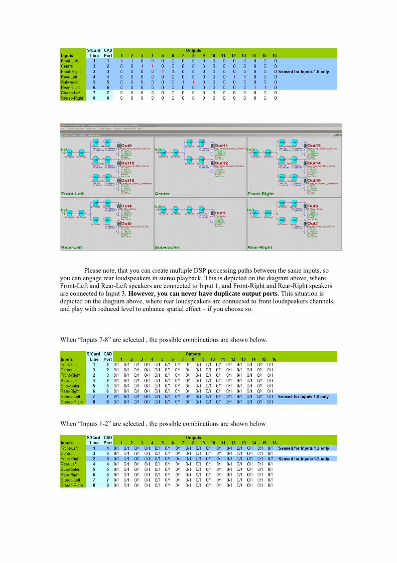
Please note, that you can create multiple DSP processing paths between the same inputs, so you can engage rear loudspeakers in stereo playback. This is depicted on the diagram above, where Front-Left and Rear-Left speakers are connected to Input 1, and Front-Right and Rear-Right speakers are connected to Input 3. However, you can never have duplicate output ports. This situation is depicted on the diagram above, where rear loudspeakers are connected to front loudspeakers channels, and play with reduced level to enhance spatial effect – if you choose so. When “Inputs 7-8” are selected , the possible combinations are shown below.

When “Inputs 1-2” are selected , the possible combinations are shown below

BBM Mode with 1-6 Inputs BBM mode is explained in the subsequent chapter, for now, it is important to realize, that Left Subwoofer and Right Subwoofer receive complex signal, which is composed of many other channels. This is why subwoofers are described as having “synthesized” signals on the diagram below.

Secondly, please note, that LFE channel (the .1 channel) from the DVD player is connected to sound card Line 5 input, and allocated to CAD Input port 5, and will be synthesized further to be played by Subwoofer 1. Subwoofer 2 does not receive direct input from the sound card. Signal for this subwoofer is completely synthesized, and CAD Input port 7 has been allocated for this subwoofer. This will work very well, as the physical sound card Input 7 is not sensed when the input mode is set to “Inputs 1-6”. Summed L+R with 7-8 Inputs

In this mode, the LFE channel (the .1 channel) from the DVD player is connected to sound card Line 5 input, and allocated to CAD Input port 5, and will be synthesized further to be played by Subwoofer 1. Subwoofer 2 does not receive direct input from the sound card. Signal for this subwoofer is completely synthesized, and CAD Input port 6 has been allocated for this subwoofer. This will work very well, as the physical sound card Input 6 is not sensed when the input mode is set to “Inputs 7-8”. Summed L+R with 1-2 Inputs

In this mode, the LFE channel (the .1 channel) from the DVD player is connected to sound card Line 5 input, and allocated to CAD Input port 5, and will be synthesized further to be played by Subwoofer 1. Subwoofer 2 does not receive direct input from the sound card. Signal for this subwoofer is completely synthesized, and CAD Input port 7 has been allocated for this subwoofer. This will work very well, as the physical sound card Input 6 is not sensed when the input mode is set to “Inputs 1-2”.

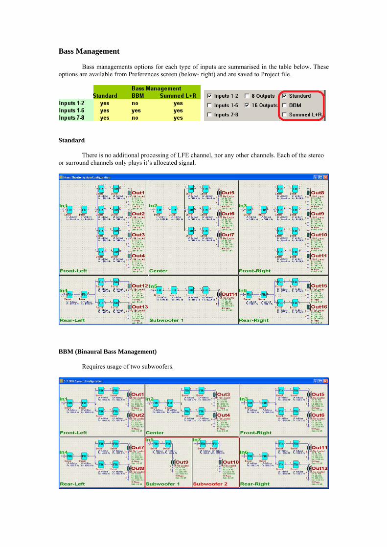
Bass Management Bass managements options for each type of inputs are summarised in the table below. These options are available from Preferences screen (below- right) and are saved to Project file.

Standard There is no additional processing of LFE channel, nor any other channels. Each of the stereo or surround channels only plays it’s allocated signal.

BBM (Binaural Bass Management) Requires usage of two subwoofers.

Theoretical foundations of this process are described in "Physiological and content considerations for a second low frequency channel for bass management, subwoofers, and LFE". AES Preprint 6628. The author reaches an interesting conclusion "….10. CONCLUSIONS The theory, informal listening experiments, and a survey of content show that: • Binaural detection by humans in the octave 45~90Hz is physiologically possible; • Music/movie VLF content exists (no new recording/mixing procedures are demanded); • High quality reproduction implies use of two channel bass management and two subwoofers (compatible with stereo, ITU 5.1/6.1/7.1, WFS, and Ambiophonics) as shown in Fig.2. In addition, several more subjective inferences follow from use of binaural bass management: • SW distortion products are ipsilateral (on the same side) as HF in main channels; • Music/movie ambience was adjudged by professionals as: "more lifelike, natural, integrated with high frequency components of the same sound in main speakers;" • Listeners were surprised; they now desire "binaural bass management" (BBM); • 2-channel LFE (i.e. "5.2") is not warranted for sparse impulsive sounds, nor at all <40Hz; • Use of two [even numbers of] subwoofers resulted in less pronounced resonance effects from room modes and supports "positional EQ" of the listening space. The standard practice of precluding redirected stereo bass reproduction is consistent with this research only in having discovered little argument favouring stereo LFE, certainly not below 40Hz, nor for main channel stereo bass <40Hz. However, for greater enjoyment of much existing and new content, there is compelling argument in recognizing significant spatial perception in the previously ignored octave 45~90Hz, and therefore for binaural bass management and subwoofers……"

The BBM is implemented as follows: Input to BBM: Left, Right, Surround Left, Surround Right, Centre, LFE. (this is the standard 5.1 configuration). Output from BBM: Left, Right, Surround Left, Surround Right, Centre, Left SW, Right SW. Where: Left SW = Left + Surround Left + Centre + LFE (all low-pass filtered <100Hz) Right SW = Right + Surround Right + Centre + LFE (all low-pass filtered <100Hz)

Left subwoofer plays all left channels filtered down to below 100Hz, and the right subwoofer plays all right channels filtered down to below 100Hz. Filtering frequency, type of filter and it’s slope is obviously selected by the user. BBM and Summed L+R level is adjusted by Page Up and Page Down keys and stored into project file.

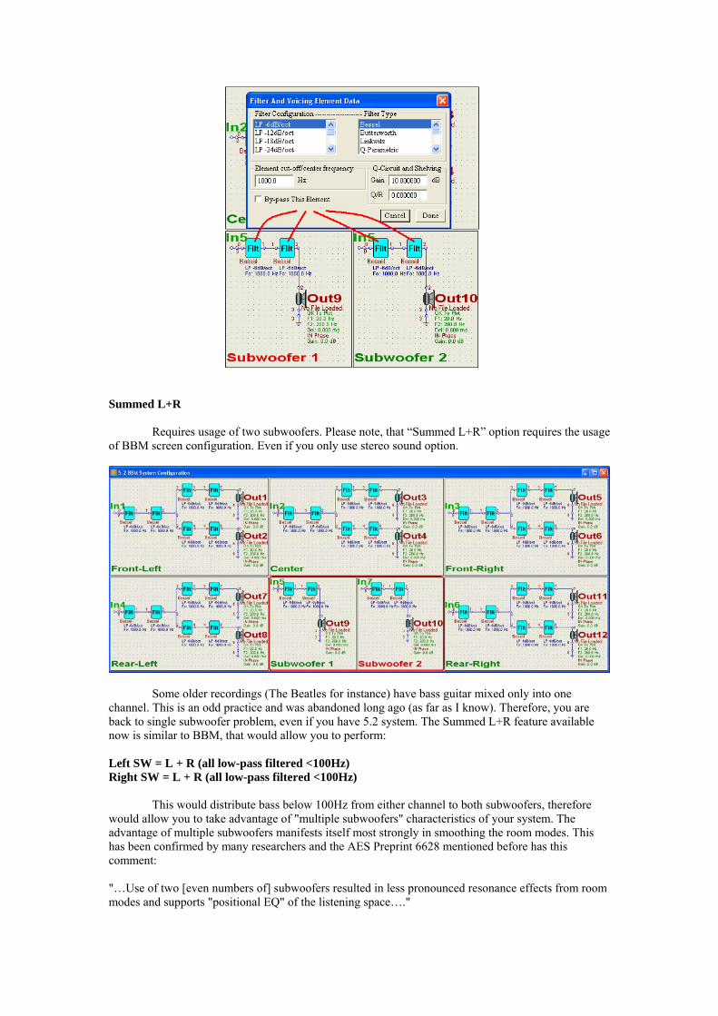
Summed L+R Requires usage of two subwoofers. Please note, that “Summed L+R” option requires the usage of BBM screen configuration. Even if you only use stereo sound option.

Some older recordings (The Beatles for instance) have bass guitar mixed only into one channel. This is an odd practice and was abandoned long ago (as far as I know). Therefore, you are back to single subwoofer problem, even if you have 5.2 system. The Summed L+R feature available now is similar to BBM, that would allow you to perform: Left SW = L + R (all low-pass filtered <100Hz) Right SW = L + R (all low-pass filtered <100Hz)

This would distribute bass below 100Hz from either channel to both subwoofers, therefore

would allow you to take advantage of "multiple subwoofers" characteristics of your system. The advantage of multiple subwoofers manifests itself most strongly in smoothing the room modes. This has been confirmed by many researchers and the AES Preprint 6628 mentioned before has this comment: "…Use of two [even numbers of] subwoofers resulted in less pronounced resonance effects from room modes and supports "positional EQ" of the listening space…."

BBM signal indication

Pink – Subwoofers Green – Left and Right channels Orange – Centre channel Blue – Rear Left and Rear Right channels Example below shows 5.2HT+BBM system with 2-way loudspeakers

And these are the channel levels for each type of input:

Input: Front-Left Channel Input: Centre Channel Input: Front-Right Channel

Input: Rear-Left Channel Input: Subwoofer Input: Rear-Right Channel

Ultimate Equalizer 19-Function Remote Control We start with a marketing pitch from: http://www.jaycar.com.au/productView.asp?ID=XC5174&form=CAT2&SUBCATID=1045#6

An all-in-one wireless keyboard and mouse solution perfectly suited to home or office PC applications. Features Qwerty keyboard and an ergonomically designed precision mouse with scroll wheel. A nano-sized USB receiver is tucked into the base of the mouse for connection to your PC. • Operating range: Up to 10m • Keyboard dimensions: 435(L) x 125(W) x 18(H)mm • Operates on the 2.4GHz spectrum • Mouse: 2 x AAA batteries (included) • Keyboard: 1 x AAA battery (included) • Supports Windows and Mac OSX

Automatic Selection of Pre-Stored Profiles Commercial HT receivers/amplifiers come with a remote control device, which allows you to switch between several input devices, be it CD-player, TV tuner, Pay-TV decoder, DVD player, etc…This is a standard feature, and is a “must have” in any home audio system. UE wireless keyboard feature perform just such function and more. Not only inputs are re-routed, but also the whole loudspeaker configuration can be re-arranged with a press of a single button. This is simply accomplished by automatically stopping the UE player, loading a pre-stored system profile, re-calculating all channel DSP characteristics, and finally re-starting the player. All these steps are automated and activated by pressing single button on the remote keyboard.

In order to assign a Profile to button “1” (second top row) on the keyboard, you must have this profile fully edited, tested, and have speakers assigned correctly too. So, please spent some time making sure, you have all your profiles perfectly edited, and voiced to your liking. You may assign up to 8 Profiles to the keyboard. Once you are happy with the sound of each profile, please go to “System Design” -> “Assign Profiles Remote”. This will open a dialogue box with 8 Browse buttons to search HD and assign your preferred Profiles (Project files) to each of the 8 data fields.

HD Path labelled “Profile 1” will be assigned to keyboard numeric key “1”. HD Path labelled “Profile 2” will be assigned to keyboard numeric key “2”. HD Path labelled “Profile 3” will be assigned to keyboard numeric key “3”. HD Path labelled “Profile 4” will be assigned to keyboard numeric key “4”. HD Path labelled “Profile 5” will be assigned to keyboard numeric key “5”. HD Path labelled “Profile 6” will be assigned to keyboard numeric key “6”. HD Path labelled “Profile 7” will be assigned to keyboard numeric key “7”. HD Path labelled “Profile 8” will be assigned to keyboard numeric key “8”. HD Path labelled “Profile 9” will be assigned to keyboard numeric key “9”. HD Path labelled “Profile 0” will be assigned to keyboard numeric key “0”.

All done!. Now, you can play UE with one profile, and then press

“1/2/3/4/5/6/7/8” key to have the whole system re-arranged and re-started. Adjusting Master Volume Master Volume control is performed remotely by pressing ARROW UP/DOWN keyboard keys. The SPL steps in 3dB increments/decrements.

Adjusting Volume of 4 Nominated Drivers (Rear Speakers) This is a very handy and often used feature. It appears, that rear loudspeakers are not mastered in the recording studios at the same level. Thus some movies/concerts are lacking the sound coming from the rear speakers, and others are correctly edited. To remedy this problem, UE allows you to nominate 4 output ports (these will be your 4 drivers in the rear speakers) in the Preferences screen – see example below.

These four ports are assigned to LEFT ARROW and RIGHT ARROW for boosting/reducing the SPL in 2dB steps. Important Note: When you first open the Preferences screen, the residual data displayed in these four fields may contain random value. Please assign your output ports to these data fields immediately.

Start / Stop UE Player This is the obvious function of starting and stopping the UE DSP engine.

HOME = Start Playback END = Stop Playback

Adjusting Volume of 2 Nominated Drivers (Subwoofers)

This is another very handy feature, and is used quite often. Subwoofers do not appear to be mastered in the studio’s recording process at the same level. Thus some movies are lacking the sound coming from the LFE channel, and others are correctly edited. To remedy this problem, UE allows you to nominate 2 output ports (these will be your 2 subwoofer drivers) in the Preferences screen – see example below.

DELETE = Subwoofer 2dB UP INSERT = Subwoofer -2dB DOWN Example of QWERTY layout

Switching Inputs With two Delta1010LT sound cards installed on the PC’s motherboard, it is possible to integrate the Ultimate Equalizer into rather extended audio system shown on the figure below. The system allows for two surround sound (5.1HT) signal sources, represented by 3D DVD player and PayTV decoder, two stereo signal sources represented by iPadTouch and Digital Radio Receiver (DAB), and in order to run full-digital processing DSP path - an SPDIF audio server, powered by Windows Media Centre or JRivers, for example.

In my final system the DAB was replaced by Western Digital PVR with stereo outputs. This is because my wife develops beautiful HD video presentations of our holidays and other events on her Mac. The presentations can be played on Western Digital with superb video and audio quality. The Concept

The main tool for re-arranging system-wide characteristics of UE is the project file. I prefer to call it a "profile", as it is essentially just that. So, you would start with setting up all parameters of your loudspeakers, filters and so on… and proceed with selecting configuration of your system in the preferences screen. This includes selecting preferred audio devices for input and output, number of inputs and outputs, sampling rate etc….Please also select "Autostart" option in the preferences screen. Once the profile has been edited and confirmed for proper operation, you need to save it as, for example, "PayTV" project file – if it was intended to work as such. Next, you would nominate this profile as assigned to keyboard button "1". So from now onwards, every time you press key "1" on your keyboard (when the UE dialogue box has the focus), UE will load profile "PayTV", calculate all filters, set all preferences parameters and will start playback automatically. You can create and assign up to 8 profiles to buttons 1-8 (see manual p112). So, single button press switches inputs and reconfigures the whole system.

The Details Selecting one of 8 input groups from each Delta1010LT sound card is accomplished by selecting Preferred Input WASAPI device. This gives you access to either sound card, and works very well, and you keep inputs' assignment as numbers between 1-8. So input "1" of the first Delta1010LT is physically different RCA line than input "1" of the second Delta1010LT. This is why input switching works. For the output, the situation is little different, because we do not want to switch the outputs while switching profiles – outputs are permanently linked to your amplifiers and speakers. Therefore, if you happened to swap preferred output devices between your profiles, you must obviously also re-assign outputs in your profiles. For instance, you have confirmed working profile "PayTV", in which Preferred Output Device 1 is Delta1010LT N#1, and Preferred Output Device 2 is Delta1010LT N#2. Then, you create another profile, in which you swapped output devices: Preferred Output Device 1 is Delta1010LT N#2, and Preferred Output Device 2 is Delta1010LT N#1. In this case, you must also swap the output assignments on the system CAD schematic. So original Output 1 must become Output 9, Output 2 must become Output 10 …….original Output 16 must become Output 8. New <-> Old 9 <-> 1 10 <-> 2 11 <-> 3 12 <-> 4 13 <-> 5 14 <-> 6 15 <-> 7 16 <-> 8 1 <-> 9 2 <-> 10 3 <-> 11 4 <-> 12 5 <-> 13 6 <-> 14 7 <-> 15 8 <->16 If you do not swap the preferred output devices, you do not need to change the output assignment in your system CAD. After that, it's just single key button press to switch between profiles (eg; switching inputs). It is not possible to advice in advance which method would work better on your particular PC. This is because your PC must meet the Pt<21.3ms and D1+D2<21.3ms conditions while running your profile. One method may work better than the other.

Delta1010LT N#1 as Preferred Input Device Surround Sound System Preferences settings are shown on figure below.

Stereo System Preferences settings are shown on figure below

SPDIF 96kHz/24bit Stereo System Preferences settings are shown on figure below.

Delta1010LT N#2 as Preferred Input Device Surround Sound System Preferences settings are shown on figure below.

Stereo System Preferences settings are shown on figure below.

Explanatory Note on Analogue Input 2 Design screen layout reflects 5.1HT system placed on the floor of your listening room as closely as possible. Therefore, we have left – centre – right design sections in the top row, and rear-left and rear-right in the corresponding corners of the bottom row. To complete all the 5.1 system channels, it seemed fit to place the subwoofer section in-between the rear speakers (which was the remaining available place on the screen). Now the design screen is easy to follow and you instinctively go to the section of the screen, which corresponds to the actual loudspeaker placement in your room. This approach was seen as a benefit to the user. However, this concept was challenged by Delta1010LT sound cards. This is because this card has line inputs 1 and 2 distinctively different from the remaining 6 inputs. Inputs 1 and 2 are balanced, have XLR connectors and provide additional 20dB gain, which can be switched off (to the same level as the other 6 unbalanced channels – at least in theory). Now, if we were to simply transfer screen indexing into physical line inputs in this sound card, we would end up with front left channel going through balanced microphone input 1, and front right channel going through unbalanced line level input 3. This brings immediate question – how accurate is gain, balancing and frequency response calibration between microphone inputs and line inputs?. Possibly quite good, but it is preferred to allocate the same type of inputs for the critical, main stereo channels 1 and 2. So, the simple solution to this was to keep screen indexing as intended, and transfer physical line channel 2 into channel 3 on the screen – that's all there is to it. When you start the program, and connect stereo source to inputs 1 and 2, you will notice, that schematic of the default crossover (2x2way) has inputs 1 and 3 and SPL meter also shows activity on inputs 1 and 3.

Ultimate Equalizer V5 in SPDIF - 96kHz/24bit all digital stereo Background

When it comes to using a HTPC as an audio music server with Ultimate Equalizer V5 running as well, you may consider fully utilizing internal sound card, with Realtek ALC889 HD audio codecs.

http://218.210.127.131/products/productsView.aspx?Langid=1&PFid=28&Level=5&Conn=4&ProdID=173 The specs are actually pretty good, with S/N =104dB for DAC. With the two Delta1010LT sound cards already installed, this is actually the third sound card you have at your disposal. Therefore, the simplest solution was to just use it. You can nominate Realtek Audio speaker system as the default player in Windows Sound system, so now, when I use Windows Media Centre (or JRivers, if you like) it will grab the internal sound card and play through it. The analogue stereo outputs from Realtek are for now connected to second Delta1010LT stereo input. Full Digital Solution

If you are interested in full digital chain of audio processing, the solution is also very simple. It is based on the ability of ALC889 to up-sample musical files played through it. Ideally, you would end up with 96kHz/24bit processing chain arranged as follows. A popular ASUS motherboard P6X58D-E has two PCI slots and digital RCA SPDIF connector. This is ideal setup for connecting the digital RCA line to Delta1010LT SPDIF connector, which is also RCA – so the connection carries digital signals (not optical).

As a side comment, I have second Windows7/64 computer, with MSI

motherboard, also running UE4 with two Delta1010LT soundcards. The motherboard is X58 Pro-E, but the SPDIF output is optical only. Here , you would have to install optical-to-digital converter, for example:

http://www.jaycar.com.au/productView.asp?ID=KC5425 ($25)

1. Start Realtek HD Audio Manager from the icons at the bottom right corner of

your Windows7 PC.

2. Choose Digital Output then Set Default Device, and Default Format as 24bits, 96000Hz – as shown below.

3. Go to Windows 7 Sound manager

The Realtek Digital Output (optical) should be already marked as “Default Device”.

4. Right-click on it to get to “Properties” control. For the P6X58D-E motherboard, you should see TWO SPDIF jacks:

5. Go to “Supported Formats” tab, and tick only 96kHz checkbox.

6. Go to “Advanced” tab, and select “2 channel, 24 bit, 96000Hz”, if not selected already. Also, clock “Apply” button is not grayed.

7. Close Windows 7 Sound dialogue.

Your Windows 7 computer is now set to up-sample music files to 96kHz/24bit format.

8. Open Delta1010LT Control Panel and make the following selections: Please note, if you have two Delta1010LT sound cards, you need to know which card is N#1 and which is N#2. Card N#1 will be connected via SPDIF of the Realtek HD on the motherboard. Card N#2 must be connected to the Word Clock output of the Delta N#1. Under ----select PCI card ------ click on the FIRST checkbox. This will select the first Delta1010LT for editing. Sample Rate = 96000Hz Buffer size = 256 (could be 512 ) Check “external – spdif”

9. Under ----select PCI card ------ click on the FIRST checkbox. This will select the first Delta1010LT for editing.

Sample Rate = 96000Hz Buffer size = 256 (could be 512 ) Check “external – word clock”

Now, your Delta1010LT sound cards are ready for 96kHz/24 bit SPDIF data stream.

10. Open Ultimate Equalizer and select Preferences screen and make the following selections:

Preferred Input WASAPI Device = SPDIF [M-Audio Delta 1010LT] Preferred Output Audio Device 1 = Multichannel [M-Audio Delta1010LT]

If you have TWO Delta1010LT sound cards, select Preferred Output Audio Device 2 = Multichannel [2- M-Audio Delta1010LT]

Check “Inputs 1-2” Check “8 Outputs”

If you have TWO Delta1010LT sound cards, select Check “16 Outputs” (NOT 8 Outputs)

Sampling Rate = 96000 Buffer Size = 2048 samples OR 4096 samples (preferred 4096)

Now your UE is also ready for 96kHz/24bit playback.

You can start Windows Media Player and UE5 and have some fun listening to your “studio quality” music.

Here is a proof, that the Realtek ALC889 HD audio codec is indeed up-sampling to 96kHz. I captured 44.1kHz SPDIF from a CD player, and 96kHz SPDIF played from the PC audio server.

44.1kHz SPDIF captured with 200ns timebase.

96kHz SPDIF captured with 200ns timebase.

Player Mode Having completed system design there is no longer need to display all design related graphs, parameters and even the system schematics. Ultimate Equalizer can now be switched to “Player Mode”, in which the program would only run DSP convolution, listen to the keyboard and display input and output SPL levels, Gain of the system, and DSP performance parameters, necessary for monitoring of your system. There are obviously Play and Stop buttons, and also the currently loaded profile’s name. Main screen is much reduced, so it only holds the Player’s control box and it’s own menu bar. Indeed, once the design phase is completed, the Player Mode should become the main operating mode of the program. The Player Mode is accessible from Playback menu item – see below. It may be beneficial to give your profiles descriptive names (<40 characters), so that you know exactly where the UE player is connected to, and at what bit rate – as in the example below.

On the top of these, all keyboard remote functions are active in Player Mode, so you can switch inputs, adjust master volume and volumes of all selected drivers, start/stop the convolution engine as usual.

To start Ultimate Equalizer in “Player Mode”, please go to Preference screen and check “Player Mode” check box. Next time you start the UE, it will enter straight into the Player Mode.

Now, the Ultimate Equalizer has made significant room for other programs,

namely, Windows Media Player or JRivers, or others to run. To exit from the Player Mode, please select “System Design” -> “Current System” menu option. The standard design screen will now be fully restored.

Appendix A: Why use a fix point measurement? The recommended measurement approach for use with the Ultimate Equalizer is to set the measurement system up and to make all SPL measurements with the microphone at a fixed position and with a fix delay removed from the data, based on the distance from the microphone to a reference point on the speaker baffle. This setup is shown in Figure A1. This setup is recommended because when each driver is measured and the same delay is removed, the phase response for all drivers will include the effects of the relative path length differences from the drivers to the measurement point. If the measurement point is along the design axis and at the design distance the measured phase response will accurately reflect the phase differences between drivers relative to the design point. Examining Figure A1, it is the delay defined by the distance from the design point to the reference point on the speaker baffle that is to be removed from the impulse response in the form of the acoustical distance shown in the MSL impulse response plot. Removing the same propagation distance from all drivers results in the phase being measured relative to the arc defining the position of equal distance from the design point. Thus, excess phase associated with the propagation distance from the driver acoustic center to this arc is retained in the phase data. When a linear phase speaker is designed using the Ultimate Equalizer the phase response is automatically linearized. If the driver phase is relative to the arc of equal distance, then the filtered drive phase will be linearized relative to the arc of equal distance. That is, the relative offsets are automatically compensated for. Thus, with all filtered drivers exhibiting linear phase response relative to the arc of equal distance to the design point, they will retain the correct phase relationships at the design point and sum correctly yielding a perfectly linear phase system relative to the design point.

Figure A1. Measurement setup.

In the case of a speaker designed as a nonlinear phase system this measurement approach allows the user to easily overlay the phase response of each driver in the Ultimate Equalizer plot screen and add the appropriate delay to each driver to compensate for the relative offsets (see the Sample Design section on Nonlinear Phase System).

Appendix B: How Does It Work? Theoretical background Here we limit the discussion to the development of the filter transfer function for a woofer as an example. Figure C1 shows the measured, on axis response of a woofer in a sealed box with the amplitude response in red and the phase in green. Excess phase from the point of measurement to some well defined reference plane, for example the baffle surface, has been removed. The choice of reference plane will be discussed subsequently.

Figure C1. Response of woofer in a sealed box. The measurement shows the irregularity of the response due to the baffle step, diffraction and other driver irregularities. The transfer function of the driver may be denoted as D(s), where s is the complex frequency, jω. In the design of the speaker we can define a target function for the low pass acoustic response of the woofer. Figure C2 shows such a target, a 2k Hz, 4th order Linkwitz/Riley low pass response, superimposed on the woofer native response. This target response is denoted as T(s).

Figure C2. Low pass woofer crossover acoustic target.

In order to bring the acoustic output of the woofer into alignment with the target function we must develop a filter with the necessary transfer function. The response of the woofer/filter combination can be expressed as (1) T(s) = EQ(s) x D(s) Since it is desired that the acoustic output of the woofer match the target only above the natural roll off of the box high pass response and, perhaps below some frequency above the low pass cut off of the target response the filter function, EQ(s), can be defined as (2) EQ(s) = T(s) / D(s), ωlow < ω < ωhigh

(3) EQ(s) = EQ(ωlow ), ω < ωlow

(4) EQ(s) = EQ(ωhigh ), ω > ωhigh where ωlow and ωhigh are somewhat arbitrarily chosen, as shown in Figure 2, based on the characteristics of the driver response. [1] Between the limits ωlow and ωhigh the function, EQ(s) can be factored into two components, (5) EQ(s) = HBT(s) x T(s), ωlow < ω < ωhigh Substituting the expression of (5) into (2) we find that (6) HBT(s) = 1 / D(s), ωlow < ω < ωhigh

Figure C3. The form of HBT(s). That is, HBT(s) is the inverse of D(s) between ωlow and ωhigh. Outside this range HBT(s) is flat. What is done next in the SoundEasy Ultimate Equalizer is to discard the phase associated with 1/D(s) and reconstruct the phase of HBT(s) over the entire frequency range using a Hilbert Bode transformation. Thus, HBT(s) takes the form of a minimum phase equalization function which flattens the response of the driver over

the frequency range between ωlow and ωhigh. HBT(s) for the present example is shown in Figure C3 and the combination of HBT(s) x D(s) is shown in Figure C4.

Figure 4. HBT(s) applied to D(s). As indicated by (5) the final form of EQ(s) is the product of minimum phase equalization flattening the drive response over a specified frequency range and a text book filter, T(s)[2]. The final output of the system is (7) O(s) = HBT(s) x T(s) x D(s) with the response appearing as shown in Figure C5 and the transfer function of the

Figure C5. Final filtered response and target. filter shown in Figure C6. As can be seen, the filter transfer function is fairly irregular in amplitude. Such a filter transfer function would be difficult if not impossible to achieve with analog active or passive filters, or with digital IIR filters. However, it can easily be emulated using FIR filters.

Figure 6. Transfer function of the woofer filter. Phase Linearization Equation 7 defines the acoustic output of the woofer/filter combination to be O(s). In general, HBT(s) and T(s) are minimum phase. D(s) is either minimum phase or minimum phase plus a delay, depending on how the reference plane for the driver measurement is defined. Therefore, O(s) is also minimum phase or minimum phase plus a delay. Here we are interested in how we can reduce O(s) to a zero (or linear) phase response. We make note of two identities. First, (8) X(s) = O(s) / |O(s)| defines a transfer function, X(s), which has the same phase as O(s) but flat amplitude response (|O(s)| is the magnitude of O(s)). Second, the inverse of X(s), defined as (9) X-1(s) = 1/ X(s) = |O(s)| / O(s) is a transfer function that has the same amplitude as X(s) but the phase of X-1(s) is the negative of the phase of X(s), or in this case, the negative of the phase of O(s). Now, (10) Z(s) = X-1(s) x O(s) = [X-1(s) x Y(s)] x D(s) where (11) Y(s) = HBT(s) x T(s) Z(s) is therefore a transfer function which has the amplitude of O(s) but with zero (or linear) phase. The terms in brackets (12) F(s) = [X-1(s) x Y(s)] represent the filter transfer function, F(s), which must be emulated through DSP using FIR filters. Since D(s) is given (obtained trough measurement of the naked woofer), and HBT(s) and T(s) are easily calculated or defined and are minimum phase, Y(s) is also minimum phase and has a casual impulse response, y(t), given by the inverse Fourier Transformation of Y(s). Thus, Y(s) can be emulated using FIR filter

techniques applied to an appropriately windowed and sampled discrete time approximation to y(t), y(n), of length N samples. Similarly X(s), while not minimum phase, does have a causal impulse response, x(t). x(t) can be likewise windowed and sampled to obtain x(n) and could also be emulated using FIR techniques. However, we are not interested in emulating X(s) but rather X-1(s). This is easily accomplished by processing the impulse x(n) in reverse order. That is, if x(n) with length, N, represents the discrete time approximation of the impulse of X(s), then x(N-n) represents the discrete time approximation to the impulse of X-1(s).

[1] The target function could include the low frequency roll off of the woofer and appear as a band pass response and the frequency limits extended to frequencies where the response was down 20 or 30dB relative to the band pass level, for example. [2] T(s) may be composed of any combination of text book filters as required.

Appendix D: Stetting Code Preferences. The Preference screen is accessed through the main File menu. The setting allow the user to select the desired sound card for input and output, control the polarity of the input and reference channels of the MSL tool and to select the colors and type and weigh.

• Be sure to select the correct, multi-channel sound card for input and output before attempting play filters designed using the Ultimate Equalizer.

• If the impulse in the MSL tool is not pointing up the polarity can be inverted for either channel by checking the appropriate check box.

• If you are using a single Delta 1010LT sound card with analog input, 8 output and 6 inputs should be checked.

• If you are using dual Delta 1010Lt sound cards with analog input, 16 outputs and 6 inputs should be selected.

• If you intend to design a stereo system using SPDIF input you must select 1-2 inputs. Select 8 or 16 output depending on whether one or two Delta 1010LT sound cards are installed. Additionally, in the sound card control panel the hardware setting must specified appropriately. Please see the section on Sound Card and PC Setting.

• If Auto Start is checked the code will automatically load the last project saved and automatically stat playback when the code is opened. This option is intended for use when the UE serves as the crossover in a more or less permanent installation of a sound system for stereo or home theater.

• Diagram off. Selecting this option automatically closes the CAD screen when play is started. The CAD screen will reopen automatically when play is stopped.

• Delay Output should be left at 200. • Plot colors are changed by clicking on the plot variable name and then using

the sliders to alter the color as desired. • Line thickness and type are selected form the pull down menus and apply only

to the clicked plot variable. 96000Hz Sampling Frequency The 96kHz sampling frequency, now available in this package, allows for better high-frequency resolution, and extends the 3dB bandwidth to about 43kHz. Selection is available in the Preferences screen. For 96kHz sampling frequency please use buffers of 2048 and 4096 sample size

Input and Output Selection

In the typical UE configuration, Inputs 1-2 selection are used for SPDIF input data. Input 1-6 are used for 5.1HT analogue connection. Inputs 7-8 and used for additional stereo signal source.

If you use only one Delta1010LT sound card – please select “8 Outputs”

option. For two Delta1010LT sound cards please select “16 Outputs” option. Selection is available in the Preferences screen.

Nominating Output Ports For Live Volume Control

During listening tests, it was have found, that LFE channel level varies quite significantly from one movie/music DVD to the next – by as much as 10-15dB. LFE setting, that seems perfect for one movie, were too much for another. UE therefore implements a feature allowing the user to nominate two outputs (presumably two subwoofers) and control their level by additional +/-20dB (in 2dB steps) during the

playback. Now, the volume level of the subwoofers is adjusted via INSERT / DELETE keyboard keys.

Similarly, you can nominate a group of 4 drivers (4 output ports) and use LEFT / RIGHT ARROW keys to control their volume level by additional +/-20dB in 2dB steps. This is intended for the 2-way rear speakers.

These features are remotely controlled, and together with the remote master volume control, it is a major user’s convenience feature of the UE system. Selection is available in the Preferences screen. 16-input and 8-input selection Users with two Delta1010LT soundcards are able to access al 16 inputs from both sound cards. Accessing inputs of Delta1010LT N#1 is accomplished by selecting the audio device as shown below.

Accessing inputs of Delta1010LT N#2 is accomplished by selecting the audio device as shown below.

Since these settings are saved into the Project file, each time you load Project file, you automatically select one of the sound cards for input.

Appendix D: Special measurement considerations. Drivers connected in parallel or series or to amplifiers of different gain. If a speaker system is to be designed which will have one or more drivers of the same type connected in series or parallel then the far field measurement procedure should be to measure the response, relative to the design point, of the drivers as they will be used in the speaker. For example, if a WMTMW speaker is being designed, once the correct MSL signal level for the measurement of the tweeter is established (the tweeter should be measured first), the midrange drivers, connected as they will be used, should be measured and the response saved in a single driver (midrange) file. Then the woofers should be measured, again, connected as they will be used, and the result stored is a single driver (woofer) file. This will assure that the relative far field sensitivity of the tweeter compared to the midranges and woofers will be correct. The near field measurements should also be performed with the drivers connected as they will be used. Since only the shape of the response of the near field SPL is required, the microphone would still be placed close to one of the midrange or woofer drivers and the diffraction model for a single midrange or woofer, correctly positioned on the baffle would be applied to correct the near field response before merging to the far field data. The system would then be designed as a 3-way using the Ultimate Equalizer. If the amplifiers to be used for each driver should have different gain or input sensitivity, then the specific amplifier to be used for each driver should be used to power the driver during the measurement stage of design. Again, once the correct MLS signal level for the measurement of the tweeter is established, that level should remain constant for all subsequent driver measurements assuring that any differences is amplifier gain, input sensitivity or driver sensitivity will be reflected in the measurements. In the most general case any speaker system should be broken down into a 2, 3 or 4 way system regardless of how many drivers are used in each bandpass. Thus, a 3 way line array may have a number of tweeters, another number of midrange drivers and yet another number of woofers. When the drivers for each bandpass are measured, they should be connected in series/parallel as they will be used and should be driven by the amplifier that will be assigned to the specific bandpass unless all the amplifiers are identical. The response for each array would them be measured and saved in a single driver file representing the bandpass.

Appendix E: Sample Design Files The files for the sample design are included with the Ultimate Equalizer package. These files include the following: Oct_13_Far.twe Tweeter far field SPL data Oct_13_merge.wfr Woofer merged SPL data Octobet_13.hif Sample case Project file These files should be placed is a folder on you PC, "C:\Speakers\Ultimate EQ Testing". You can then open the Project file and the driver should be loaded correctly. If you place the drivers in a folder of a different name when the project file is opened you will have to browse the correct folder to load the driver files. The near and far field woofer SPL files are provided so that you may experiment with merging the data.

Appendix F: Sound Card and PC Sound Setting Sound Card For satisfactory operation of the Ultimate Equalizer software the Delta 1010LT sound card(s) and PC Sound setting must be set correctly. The Delta 1010LT sound card has a built in microphone preamplifier associated with input channels 1 and 2. This microphone preamplifier must be disabled before installing the Delta 1010LT. This is accomplished by repositioning jumpers on the Delta 101 LT printed circuit board. Please refer the Delta 1010LT manual for instruction on disabling the microphone preamplifier. Input channels 1 and 2 also used XLR connectors. It will be necessary to either purchase or fabricate XLR to RCA adapters to facilitate RCA input connections to channels 1 and 2. After installing the Delta 1010LT open the M-Audio control pane, and select the Hardware tad as shown in Figure F1. The setting should be as shown.

Figure F1. Delta 1010LT control panel. When using the analog inputs to the Delta 1010LT: · Sample Rate: Set to 48000/96000 · Buffer Size: Set to at least 128 / 256 / 512. · Mode: Set to consumer. · Data Type: Set to audio. · Emphasis: Not indicated. · SCMS: None. When using SPDIF input: · Set the sample rate to match that of the input (44.1K for CD). · Set the sync source to External-SPDIF

PC Sound · Open the PC Control panel and select Hardware and Sound. · Under Sound, select Manage Audio Devices. · When the Sound dialog open select the Playback tab. The dialog will look as shown in Figure F2.

Figure F2. Sound dialog Sound tab. · Highlight Multichannel, then click Set Default.· Click Properties and select the Advanced tab. The display should appear as shown in Figure F3.

Figure F3. Multichannel Properties Advanced tab (playback). · Set the sample rate and bit depth to 10 channel, 24 bit, 48000 Hz. · Click the Levels tab and make sure the level is set to 100. · Click Ok. · Now select the Recoding tab in the Sound dialog. The Dialog should appear as shown in Figure F4.

Figure F4. Sound dialog Recording tab. · Highlight Multichannel and click Set Default. · Click Properties and select the Advanced tab. The display should appear as shown in Figure F5.

Figure F5. Multichannel Properties Advanced tab (recording). · Set the sample rate and bit depth to 12 channel, 24 bit, 48000 Hz. · Click the Levels tab and make sure the level is set to 100. · Click Ok. · Select the Sounds tab in the Sound dialog and set the Sound Scheme to No Sounds· Click Ok to close the dialog.

Appendix G: Optimization of DSP engine It may be beneficial to understand the relationship between sampling rate, latency, UE buffer size, Delta1010LT buffer size and UE timing figures: Pt, D1 and D2. For SPDIF digital audio stream you need to use 44100Hz sampling rate. Studio quality signals are processed with 48000Hz sampling rate, and the latest “mastering quality” requires 96000Hz sampling rate. Please note, that in order to take full advantage of 96kHz sampling rate, you would have to employ tweeters operating up the 45kHz and above and measurement microphone with at least 50kHz bandwidth. If your AV setup requires low latency, you may select 48kHz/1024bin or 96kHz/2048bin settings of the UE. Improvements in low-end resolution can be accomplished by selecting 48kHz/2048bins or even 48kHz/4096bin buffers. The widest processing bandwidth will be accomplished by setting 96kHz/4096bin parameters. Sampling Frequency [Hz]

UE Buffer Size

44100 48000 96000

1024 bins

MP Latency 75ms, LP Latency 165ms,

Use for SPDIF

MP Latency = 65ms, LP Latency = 145ms,

Lowest Latency NOT ALLOWED

2048 bins

MP Latency 155ms, LP Latency 320ms,

Improved low-frequency resolution,

Higher Latency

MP Latency = 125ms, LP Latency = 290ms,

Improved low-frequency resolution

MP Latency = 65ms, LP Latency = 145ms,

Low Latency

4096 bins

MP Latency 310ms, LP Latency = 640ms, Best low-frequency

resolution, Highest latency

MP Latency 250ms, LP Latency = 580ms, Best low-frequency

resolution, High latency

MP Latency = 130ms, LP Latency = 290ms,

Improved low-frequency resolution,

Medium latency

Controlling two sound cards is best explained on the diagram below. This example is based on 48kHz/1024bin settings. Input data blocks are delivered to UE by the sound card driver every 21.33ms, and signalled “Input Buffer Full”. Once this data block is received by the UE algorithm, it can be processed within processing time Pt=9.4ms. The thread responsible for processing input blocks (Tr1) signals to the thread responsible for processing Delta1010LT N1 (Tr2), that data is ready for output, so Delta’s thread starts the process, and the data shows up on the sound card output within D1=1.5ms. From now onwards, the Tr2 thread also runs with 21.33ms interval. Finally, this thread signals to the thread responsible for the second Delta1010LT (Tr3), to start outputting data as well. Tr3 takes D2=10ms time to set up and run, and from now onwards, the Tr3 thread also runs with 21.33ms interval. Since there is 10ms lead time on the Tr2, the data in Tr2 is automatically delayed by D2=10ms.

For this whole scheme to work, we need to following to happen:

1. Pt < 21.33 ms. This is obvious, otherwise the CPU takes too much time to process one block of data before the next block arrives.

2. D1+D2 <21.33ms. Actually D1+D2 should be much less than 20ms to be on the safe side. If not, that the next, newly calculated convolution block is signalled for output, but the sound cards are still busy processing the previous block.

ASUS

Motherboard

96kHz/2048 UE buffer

Delta1010LT buffer setting

Pt D1 D2

128bins 4.5 1.6 10.5 256bins 4.5 4.4 10.8 512bins 4.5 6.9 12.8

48kHz/2048 UE buffer

128bins 9 4.3 10.3 256bins 9 6.9 13.8 512bins 9 6.9 13.6

48kHz/1024 UE buffer

128bins 4.4 3.5 11.5 256bins 4.4 6.1 13.8 512bins 4.4 6.1 13.9

96kHz/4096 UE buffer

128bins 21 1.2 10.1 256bins 21 3.2 10.6 512bins 21 5.4 14.1

The spreadsheets above and below show two rows highlighted in red – this is where D1+D2 are too close to 20ms, and are not recommended settings. It is recommended, that you characterize your system by trying different settings and then testing the sound for stability. For instance, you can Start/Stop the player in 10second intervals and record Pt, D1, D2, and compare these figures for stability. Test results from two motherboards show differences in performance, even tough both computers run Windows7/64bit and the same sound card drivers.

MSI Motherboard

96kHz/2048 UE buffer

Delta1010LT buffer setting

Pt D1 D2

128bins 4.5 1.1 8 256bins 4.5 3.7 5.7 512bins 4.5 6.2 11.5

48kHz/1024 UE buffer

128bins 6.6 2.7 8 256bins 6.6 9.3 8

Bodzio Software office runs one computer with ASUS motherboard, i7 960, with Windows7/64bit in 96kHz/2048bin mode, and another computer with MSI motherboard, also i7 960 with Windows7/64bit in 48kHz/1024bin mode. Both machines display the same latency and good sonic performance.

More exact process flow of the UE audio threads is shown above. Audio processing inside the UE software is handled by several parallel “software threads”. There is one capturing thread and two rendering threads. All threads are invoked at the same time, but both rendering threads are initially in the “wait” state. Once the capturing thread finished initialization process, it semaphores to Delta N#1 to start it’s rendering initialization, and then goes into the “wait” state too. Once the first Delta has completed initialization, it triggers the second Delta card for rendering initialization and goes into “wait” state itself.

During the initialization process, only one thread is communicating with Windows WASAPI resources, thus preventing any possible collision between the threads. When the second rendering thread finished initialization, it will release capturing thread from it’s “wait” state (via semaphore), so that the first block of data can be captured and processed by the convolution engine. The second Delta rendering thread goes into the “wait” state itself too.

As soon as the calculated data is available, the capturing thread triggers the

first Delta to actually start rendering, and this process in turn, triggers the second Delta to start rendering too. From now onwards, all three threads run in their own processing loops.

Loop timing depends on the sampling rate and UE buffer size. For example,

with 1024bin buffer size and 48kHz sampling frequency, the loop time is 21.334ms. Delta1010LT buffer size is also influencing some timing within the loop –

plainly speaking, it’s eating away loop time. Buffer size Delay [ms]

1024 21.334 512 10.667 256 5.335 128 2.667 64 1.334

Delta1010LT buffer simply adds delay to the processing of audio blocks. For

instance, assume we run with 48kHz and 1024bin UE buffers, resulting in 21.334ms loop time. Delta1010LT’s buffer size of 256 will add 5.335ms to the audio processing loop, and this is quite significant delay in comparison with other contributing delays, as the convolution processing itself may take only 5ms.

When optimizing the DSP performance of your setup, you need to take this

information into account. For instance, Windows 7/64 with i7 960 CPU seems to be optimized for the following parameters:

Sampling frequency = 48kHz Delta1010LT buffer size = 128 UE buffer size = 1024 Pt = 5ms << 21.334ms For the above settings: D1 = 3 – 4, D2 = 13 - 14 Therefore, D1 + D2 = 18(max) < 21.334ms. Selecting Delta1010LT buffer of 256 would result in extra 2-3ms delay, and

this would bring D1+D2 dangerously close to 21.334ms. In cases like this you may see “Synch” instead of “D2=xx.xx” displayed by UE, and telling you, that the system may not be able to time align the second Delta1010LT. A solution to this would be to set UE buffer to 2048bins, so that loop time would increase to 42.667ms.

Appendix H: PC Firmware Recommendations Simple Configuration: Minimum Requirements: The Ultimate Equalizer has been tested for satisfactory operation on this minimum, off the shelf PC, configuration: CPU = 2.7 G Hz AMD Sempron 140 Processor Mother board with one open PCI expansion slot for Delta 1010LT sound card installation. RAM = 2 Gb. Operating System = Windows 7 Home Premium 64 bit. Sound Card = Single Delta 1010LT allowing 6 analogue or 2 SPDIF input and 8 analogue output Advanced PC Configuration: Computer: CPU = Intel Core i7 960 3.2GHz, LGA 1366. It is recommended to use more advanced CPU as future upgrades of the Ultimate Equalizer may include 96kHz and 196kHz processing of 24-bit digital streams. Multi-core CPU may be required. Motherboard = with 2 PCI slots, such as GIGABYTE GA-EX58-UD4P, MSI X58-PRO-E X58 DDR3. It is currently necessary to use motherboard with 2 PCI slots for 16 output option. If you only use 8 output option, then a motherboard with single PCI slot is adequate. RAM = 4Gb. This amount of RAM should be sufficient to run Windows7/32bit efficiently. HD = Patriot 128Gb SSD, 128Mb buffered (SSD memory HD). As your system may be exposed to significant vibrations coming from subwoofers, it is beneficial not to have traditional, spinning, hard disk drives. Operating System = Windows 7 Professional, 32bit, SP1. This operating system is necessary if you need to run 16 output option with Marian sound cards. This is because at the time of writing, there is only Windows7/32bit driver available for the Trace8 and TraceOut A16 sound card. If you intend to use Delta1010LT sound cards, you can use Windows7/64bit operating system. Monitor = LG E1941T. This is probably the smallest monitor that would work with UE graphics system. Any contemporary monitor should work. Power Supply = Good quality, low noise, low ripple within 10Hz-20MHz bandwidth is recommended. The following website may assist you in selecting the PSU.

http://www.hardwaresecrets.com/page/power/15/1 Please note, that power supply may be located just below PCI slots. This may induce EMI noise into to one of the soundcards. Some additional filtering and shielding may be required. Please visit: http://techgage.com/article/asus_xonar_d2_sound_card/http://www.murata.com/products/emc/case/computer/pdf/d_1.pdf Sound cards: For input = Delta1010LT Please visit: http://www.m-audio.com/products/en_us/Delta1010LT.html Driver = Delta Series Installer 6.0.2 - Driver: 5.10.0.5074 for Windows7/64. Delta1010LT is being used with Inputs 1-6. Please note, that Input 1 and Input 2 are microphone, XLR-type inputs with higher gain. You will need to move 4 jumpers on the sound card to convert these inputs to “line level” inputs. Also, you can buy XLR male-to-RCA female adaptors to standardize all 6 input lines to RCA-type. For output = Delta1010LT – this is sufficient for 8-output configuration. Delta Series Installer 6.0.2 - Driver: 5.10.0.5074 for Windows7/64bit. For 16-output configuration, you will need two Delta1010LT sound cards. Sound Processing Configurations: Input Configurations: 2 analogue inputs for stereo input signals. 6 analogue inputs for 5.1 HT system Output Configurations Any of the 8 Analogue Outputs of Delta1010LT Any of the 16 Analogue Outputs of two Delta1010LT. Here is a summary of possible configurations Windows OS: Delta410 – 2in/8out – Windows 7/64, Windows 7/32. Delta1010LT - 2in/8out – Windows 7/64, Windows 7/32. Delta1010LT - 6in/8out – Windows 7/64, Windows 7/32. Delta1010LT + Delta1010LT - 6in/16out – Windows 7/64, Windows 7/32 – motherboard needs 2xPCI slots. Please make sure, you use correct drivers for your operating system for the Delta1010LT sound cards.