MASTER THESIS

AUGMENTED GRAVITY MODEL: INSTITUTIONS,

INFRASTRUCTURE AND GLOBALIZATION IMPACT ON

BILATERAL EXPORTS AMONG OECD COUNTRIES.

AUTHOR: TOM SCHOLTES

STUDENT NUMBER: 476859

ABSTRACT

This thesis investigates the influence of Institutions, infrastructure, and globalization on bilateral aggregate

exports among countries that belong to the Organization for Economic Cooperation and Development

(OECD). This thesis applies the gravity model for the period between 1995-2018 and uses fixed-effects

with the Ordinary Least Squares (OLS) estimation method. After ensuring that estimations pass the RESET

test for misspecification, this thesis observes a positive relationship between bilateral aggregate exports and

when the reporter and partner country are both members of the European union or regional trade agreement.

Moreover, the bilateral aggregate exports are higher among countries that have a common currency. This

thesis's novelty is assessing exporter's economic and political globalization, state fragility, and the impact

of exporter's innovation on bilateral aggregate exports. The results suggest that economic, political

globalization, and exporter's innovation indexes positively contribute to increase bilateral aggregate

exports; conversely, state fragility affects exports negatively. The institutional and infrastructure quality

indicators reveal a mixed impact on bilateral aggregate exports, with road infrastructure quality having a

substantial positive impact on the dependent variable. The most perplexing results stem from the negative

impact of an increase in political stability and market openness on bilateral aggregate exports.

TABLE OF CONTENTS 1. Introduction 1

2. Literature Review draft 3

2.1 Historical overview of the theoretical framework 3

2.2 Determinants of bilateral trade flows 5

2.3 Extension of the gravity model 7

2.4 Top three errors 11

2.5 Hypothesis and conceptual framework 12

3. Data 13

4. Methodology 15

4.1 Gravity model equation 15

4.2 Econometric Specification 16

4.3 Linear estimation method 17

5 ANALYSIS 19

Diagnostics 19

6. Results and discussion 22

6.1 Interpretation of main table 22

6.2 Interpretation of the robustness table 24

6.3 Brief summary table 25

6.4 Limitations: 26

7. Conclusion 27

References 28

APPENDIX: 36

Main Table 36

Robustness Table 37

A: Data 38

B: Diagnostics (main table) 45

D: Results and discussion 54

E: Diagnostics for Robustness Table 56

G: Theoretical foundations of Gravity model 65

H: Traditional Specifications 65

I: Variable Information 68

1

1. INTRODUCTION

Natural sciences, such as biology or physics possess directly intuitive and hard scientific characters, these

qualities have attracted social and economic sciences to adopt these relations or “laws” from natural

sciences. Multitudes of examples can be found effortlessly — The use of logistic functions for technological

diffusion originating from epidemic laws to Goodwin’s growth cycles inspired by the dynamics of the

biological system called the "prey-predator" model. From an empirical point of view, for economists, results

of this adoption have been successful. The results of most empirical studies maintained a solid ground under

various econometrics test employed to verify the robustness of these adoptions. Econophysics is defined as

an interdisciplinary research field, which, to solve a problem in economics, applies methods and theories

initially developed by physicists (Kutner et al., 2019). Jan Tinbergen was the first to obtain a Nobel Prize

in Economics in 1969, adapting Newton's law of gravitation by replacing the mass with Gross Domestic

Product (Garlaschelli, 2014) and the distance between masses with the distance between countries.

The gravity equation is known to be one of the most prominent empirical economic model; Using a single

equation in which coefficients are statistically well defined and economically sound, the variations are well

explained. (Frankel and Rose, 2002). The gravity equation has therefore been widely used to explore the

determinants of bilateral trade flows. Early debates until the nineties focused on solving the theoretical

framework after being hit by waves of skepticisms, detailed information on theoretical framework is found

in the first sub-section of section two. The ongoing debates mostly focus on evaluating various estimation

techniques performance.

Trade is seen as an engine of economic growth (Senhadji & Montenegro, 1999), thus, it is important to

assess the impact of institutions, the quality of infrastructure and the impact of economic and political

globalization on OECD countries' bilateral aggregate exports. The divergence in results from numerous

papers findings on export determinants spurred curiosity on choosing this topic for the master thesis.

Differences in outcomes befall due to heterogeneity in time-periods, sample sizes, and research models

used for the study. This research study performs a comprehensive examination of the possible factors or

determinants of OECD countries' trades using the data from 1995 to 2018, employing the gravity model

with the traditional OLS estimation method. Besides commonly considered variables of gravity model

GDP, Distance, and regional trade agreements, this research study expands its study to other factors,

including OECD countries' stock FDI, exchange rate, EU, and common currency. Additionally, various

standard dummy variables of trade costs are added to natural, manmade, and cultural differences.

There are at least two reasons, from a theoretical standpoint, how institutions can have a direct impact on

trade. First, the quality of institutions acts as trade impeding or enhancing factors on bilateral trade,

influencing the cost of international exchange, e.g., insecurity decreases the bilateral export volume by

reducing the quantity of exports. Second, institutions are the origin of comparative advantage.

Borchert and Yotov (2017 ) claim that globalization can be seen anywhere but in estimates utilizing gravity

model, discovering that manufacturing trade is affected by globalization. However, these authors did not

measure globalization using clear, explicit indicators; authors interpret the change in magnitudes of

distance, RTA, and contiguity impact on trade as proxies for economic globalization. This thesis examines

the impact on global trade of political and economic globalization indexes. There are two dimensions of

economic globalization in the employed index: economic flows, restrictions on capital and trade. The

2

economic flows sub-index contains trade, FDI, and portfolio investment data. The Restrictions sub-index

acknowledges obscure import barriers, international trade taxes (as a share of current income), average

tariff rates and an indicator for capital controls. Political globalization is based on the number of high-level

commissions and embassies in a nation, the number of UN peacekeeping missions in which a country has

participated, the number of international institutions to which a country belongs, and the number of bilateral

or multilateral treaties signed. Borchert and Yotov (2017) conclude that further research needs to be

conducted on globalization's influence on trade. The results of this thesis indicate significantly positive and

substantial influence of economic and political globalization on aggregate bilateral exports for the full

period (1995-2018) and the shorter period (2011-2018).

This thesis finds that bilateral aggregate exports are higher among European Union members, Regional

Trade Agreement, and when countries export to a partner with a common currency. In addition, this thesis

obtains mixed results regarding the effect of institutional variables, where, when the entire period is

regarded (1995-2018), the rule of law and government size have a positive impact on exports. Conversely,

political stability and market openness, have an adverse impact on aggregate bilateral exports. The influence

of soft infrastructure, namely the internet usage and mobile subscriptions index, which is an indicator for

the Information and Communications Technology (ICT) index, positively impacts the bilateral aggregate

exports. Contrary to expectations, the impact of total infrastructure investment on the dependent variable is

significantly close to zero. This thesis also finds that importers' average weighted Most Favored Nation

(MFN) tariffs harm the bilateral aggregate exports. Preliminary evidence using a recent period (2011-2018)

with alternative variables for the institutional and infrastructure quality indicate that the state fragility index

is negatively related to exports. The exporter 's innovation index, by contrast, has a beneficial impact on

exports. Alternative infrastructure quality variables using indexes for the quality of port, road , rail and air

transport indicators reveal that exports are significantly affected only by the port and road infrastructure

indexes. The port infrastructure improvement hurts exports while the road infrastructure doubles in terms

of magnitude of the impact and switches signs to positive.

The thesis is set as follows: The following section initiates with a historical overview of the theoretical

framework (2.1) subsequently, followed by presenting the main determinants of trade found in the literature

(2.2) then subsequently narrows focus on institutions, infrastructure and the impact of globalization on

bilateral trade flows in sub-section 2.3. The last sub-section (2.5) of section 2 states the objective of the

research, hypothesis and summarizes variables investigated in the main and alternative specification

(robustness table). The third section describes the data, while the section four explains the methodology by

providing the gravity equation, econometrics specification and a summary of the benefits of using Ordinary

Least Squares (OLS) with fixed effects. The fifth section is about the diagnostics, examines the data

structure and pre-estimation tests are conducted. Subsequently in section six, output interpretation of the

regression results of the main and robustness table are presented. Subsections 6.3 and 6.4 summarizes the

main findings illustrating the constraints of the study and provides suggestions for further research. The last

section (7) ends with a conclusion.

3

2. LITERATURE REVIEW DRAFT

2.1 HISTORICAL OVERVIEW OF THE THEORETICAL FRAMEWORK

Tinbergen(1962), in his seminal work, introduced the gravity equation by using the analogy of the

Newtonian gravitation theory, which approximates bilateral trade flows around two nations. Planets, by

their sizes and proximity, are mutually attracted. Trade is similarly commensurate with nations' respective

Gross Domestic Products (GDP) and geographical vicinity. Alternative micro-foundation was employed

by Arango (1985) for the earliest applications to the economics of Newtonian law of gravity, studying the

immigration flows.

In finding theoretical and economic foundations for the gravity equation with Constant Elasticity of

Substitution (CES) assumption and differentiation of goods by origin, Anderson(1979) is the pioneer,

highlighting the significance of the general equilibrium effects of trade costs. Anderson (1979) carried out

the initial effort to derive the gravity equation from the theoretical model using the Armington assumption

in which goods are differentiated by place of origin with the expenditure system of Cobb Douglass where

each good is produced by one nation. The reduced form of bilateral trade was subsequently derived by

Bergstrand (1985) utilizing CES preferences over the assumption by Armington of differentiation of goods.

Bergstrand (1985 and 1989) demonstrates that the theory developed by Paul Krugman (1980) of

monopolistic competition is the gravity model's direct implication. Bergstrand (1990) replaced product

differentiation by the provenance of a product with product differentiation between producing companies

based on the assumption of monopoly competition, introducing prices into the model and the hypothesis of

Linder. In Krugman's model, consumers' preference for a variety is why identical firms trade differentiated

goods. Armington models have an undesirable feature, which assumes that goods are differentiated by

production location. The monopolistic competition serves to overcome this aspect. Each country specializes

in producing different sets of goods, and the firm location is endogenously determined.

In the past, eminent international trade models included the Hecksher-Ohlin model (Bergstrand, 1985;

Deardorff, 1998), which relies on differences in factor endowments between countries as a justification for

trade. Deardorff (1998) demonstrates that trade is explained by conventional factor proportions, which in

turn explains the gravity model. In addition, Deardorff (1998) also reveals that the long-established

Heckscher-Ohlin-Samuelson framework with full country-level production specialization and

homogeneous goods could also derive the gravity equation's fundamental form. On top of the monopolistic

competition assumption, Helpman (1987) derived the premise for the assumption of increasing returns to

scale with product differentiation at the company level. The new and old theories were mediated by

Deardorff (1998) through asserting that the gravity equation could be extracted from standard trade theories.

The gravity equation obtained from Helpman's (1987) monopolistic competition was used by Hummels and

Levinsonhn (1995) to estimate bilateral trade of OECD countries trading differentiated manufacturing

products. The simple model explained 90 percent of the variation in trade flows among OECD countries

with the assumption that goods were differentiated. After the random selection of non-OECD countries, the

post-robustness check concluded that the variation in flows of trade among these countries was similar to

that of OECD members, leading to the verdict that hidden factors drive the empirical success of the gravity

equation in its rudimentary form.

The gravity equation also arises from the Ricardian sort of model. The Ricardian model rests on

technological discrepancies across countries to explain trade. It was previously assumed that models from

4

Heckscher-Ohlin and Ricardian could not provide a basis for the gravity model, i.e., the power and stability

of the gravity equation to explain bilateral trade flows. Eaton and Kortum (2002) produced the most eminent

structural gravity theory in economics, deriving gravity from a Ricardian structure with intermediate goods

on the supply side.

Chaney and Helpman (2008) acquired the gravity equation from international trade theory wherein firms

are heterogeneous, and trade differentiated goods. Specifications and variables employed in the model

ought to be derived from economic theory1, thereby drawing appropriate inferences from estimations using

the gravity model. This requirement of having solid theory backed empirical models rationale motivated

various researchers to build a solid theoretical foundation of the gravity equation (Bacchetta et al., 2012).

A range of trade theories may give rise to gravity models (Feenstra et al., 2001; Evenett and Keller , 2002;

and Feenstra, 2004). Feenstra et al. (2001) argued that on exporter-importer nation-size factors, diverse

theoretical models predict dissimilar elasticities, which depended on whether products were differentiated

or homogeneous. Anderson and van Wincoop (2003) based the hypothesis of product differentiation with

respect to their place of origin, creating an augmented model of Anderson (1979). Differentiated products

indicate that a surge in the exporter 's revenue has a greater proportional effect on exports than the domestic

market effect, with homogeneous goods having a reverse effect on the domestic market. The primary

contribution of Anderson and van Wincoop (2003) is the addition into the original Anderson (1979) model

the multilateral resistance terms for the sender and the recipient that proxy for undetected trade barriers to

exist, especially emphasizing the role of heteroskedasticity. As assumptions Anderson and van Wincoop

(2003) employed CES, model of monopolistic competition with solitary economy. Melitz (2003)

highlighted the diversity of companies in terms of their export behaviour. Catalyzing the theoretical

foundation for the presence of zero trade flows in the data. Helpman et al. (2008) with selection on which

markets to enter as heterogeneous firms and these authors introduced a two-stage estimation process that

factors in extensive and intensive trade margins and is responsible for setting up a framework that justifies

the existence of zero trade flows. Chor (2010) and Costinot et al. (2012) with Ricardian model on sector

level. Unresolved empirical application problems of the gravity equation were unraveled by Garcia,

Pabsorf, and Herrera (2013). The dataset of authors covers 80 percent of world trade using the gravity

equation predicated by the theoretical model of Anderson and van Wincoop (2003), a wide range of

estimators are compared, claiming that in the presence of heteroskedasticity non-linear estimators produce

more accurate results. They conclude that, when zero tade flows are present, the Sample Selection Model

of Heckman and Poisson Pseudo-Maximum Likelihood (PPML) are the leading models for the gravity

equation specification. Inclusion of export probability as a first step to circumvent the gravity parameter

estimation inconsistency caused by sample selection bias due to zero trade flow values. Asset accumulation

importance using dynamic framework (Olivero and Yotov ,2012; Anderson et al., 2015; and Eaton et al.,

2016). For a broad class of general equilibrium models of trade, Allen et al.(2014) demonstrated the

uniqueness and existence of the trade equilibrium that derives adequate conditions for gravity's prevalent

power. Caliendo and Parro (2015) link the gravity model to sectoral input-output framework. Armington

model applied to sector level trade data by Anderson and Yotov (2016).

1 Summary figure of the main theoretical foundation pillars of gravity model can be found in the Appendix G (Figure 8)

5

2.2 DETERMINANTS OF BILATERAL TRADE FLOWS

For decades, the identification of primary sources of international trade flows has been a topic of significant

interest to academics. Wang, Wei, and Liu (2010) include Foreign Direct Investment(FDI) stocks, Research

& Development (R&D) proxy, factor endowment similarity. The authors obtain highly significant results,

although the authors did not include trade costs except geographical distance. Cieslik (2009) formally

obtained the assumption of complete specialization is an insufficient prerequisite for the use of incomplete

specialization models from monopolistic and neoclassical competition to obtain the gravity equation.

Cieslik's (2009) findings show that factor proportions and country size variables are key determinants of

bilateral trade mass; The impact of these determinants is model-specific. The researcher concludes that if

there is variation of relative factor endowments between partners, ignoring the factor endowments can lead

bias caused by omitting variables considered to be important. The complete specialization assumption, as

the study indicates, may be appropriate for developed economies, in this thesis, the largest OECD countries

are considered, thus the appropriate assumption is of complete specialization as the sample mostly includes

developed countries. When low and middle-income countries' trade is examined, the incomplete

specialization assumption is appropriate.

A positive association between bilateral trade flows and the total population of a country is reported by

Matyas (1997). Through a higher population leading to greater import demand. Research results from

Bendjilali (2002) contradict the results of the aforementioned Matyas (1997), indicating that a larger

population leads to bulky domestic market as well as a smaller export market or a larger import market.

Other authors present different results (i.e., Brada and Mendez, 1983; Pelzman, 1977). The general

agreement among scholars is that the population and bilateral trade flows are positive.

To evaluate the European Union and Mercosur trade, Lehmann and Zarzoso (2003) utilized the gravity

model and attempted to assess the possible impact of agreements of trade among these two trade blocs. A

panel data was used to analyse the effects variables that do and do not vary over time on a sample of 20

countries. Authors state that the Random Effects model is less preferred than the The Fixed Effects model.

Authors find exchange rates, infrastructure, and income differences to be substantial determinants of

bilateral trade flows. Lehmann and Zarzoso (2003) utilize a Two-step estimation to estimate dummy

coefficients and time-invariant parameters in a fixed-effects model.

Franker and Rose (1998), Rose (2000) estimate that monetary unions induce trade. This theory has led to

the creation of the Optimum Currency Areas (OCA) concept of “endogeneity”. Over time, European

Monetary Union progresses into OCA Franker and Rose (1998). Rose and Stanley (2005 ) indicate that the

introduction of the euro has a significant and highly significant impact on trade between the members of

the EMU, and

that the combination of these estimates signifies an 8-23% increase in trade during its first years of creation.

Rose (2017) estimates that when the sample includes more than just EMU countries, the euro 's influence

on trade is even more substantial. Micco et al . ( 2003) found that, based on the membership of the EMU,

the EMU encourages trade by 8 to 16 percent, and this effect has been growing steadily. Serlenga and Shin

employ gravity equation to estimate the impact of European Monetary Union (EMU) for 15 european union

member states. They do not recognize a significant impact from EMU membership, they realise the time

frame of the sample ending too soon (in 2001). By means of expectations, trade costs, and friction reduction,

6

Bergin and Lin(2012) find that the EMU has a significant effect on trade. Camarero, Herrera and Tamarit

(2018) conclude that economic approaches and dataset dimensions largely influence results.

Camarero Herrera and Tamarit (2018) investigated the impact of the euro on trade with 28 countries while

using 1990-2013 period making the use of gravity model. To correct any possible bias that potentially arises

from unobserved time-varying heterogeneity or multilateral resistance variables (Baldwin and Taglioni,

2006). Authors include time-varying fixed effect in their gravity specification. Furthermore, Camarero

Herrera and Tamarit (2018) investigate if FDI and trade are substitutionary or complementary by including

inward and outward stocks into their specification. Researchers conclude that Foreign Direct Investment

(FDI) has a strong positive impact on trade, stating that omitting FDI would bias the euro's introduction

upward.

There is a lack of strong agreement among studies that recognize the influence of cultural distances on

trade. A positive relation between cultural distance and trade is reported by Guiso et al . ( 2005), while

Tadesse and White (2007), Linders et al. (2005) and Boisso and Ferrantino (1997) report that trade is

inhibited by greater cultural distance. It is therefore desirable to understand how cultural divergences

between people in different countries can affect the successful completion of transactions.

Many scholars have researched the effect of exchange rate fluctuations on international trade, discovering

that in reaction to the lower risk-adjusted expected earnings they are confronted, literature expects traders

to turn their attention to the domestic market if traders are risk-averse, or if hedging is too expensive, or

even impractical (Thursby and Thursby ,1987; Akhtar and Hilton, 1984). As a result, Arize (1997 ) notes

that a rise in fluctuations in the exchange rate contributes to a decrease in trade. Chowdhury(1993) states

the absence of a clear consensus on this matter. A beneficial relationship between trade and exchange rate

fluctuations is pointed out by Sercu and Vanhulle (1992). In this case, trade is considered an option held

by the firm, emphasizing that with volatility, the option's value can rise.

Further studies highlight the substantiality of risk aversion of the traders. The results from Doğanlar (2002)

indicate that export volume and exchange rate volatility are negatively related since this variability

negatively affects the expected marginal utility. Froot and Stein(1991) was the initial advocate to debunk

the common belief that the exchange rate would not have a significant role in the FDI decision of an MNE.

Before this work, the assumption was that an increase in domestic currency value would lead to cheaper

costs, which would lower nominal returns in the home currency (Blonigen, 2005). In this way, the

advantages and disadvantages would counteract each other. Empirical evidence provided by Froot and

Stein(1991) reveals that currency appreciation leads to an increase in FDI activities of MNEs. In imperfect

capital markets, internal capital is more costly to borrow via external sources than within the firm.

Consequently, wealth is straightaway impacted by the exchange rate. Withal, Cross-border acquisitions

increase with the depreciation of the home currency. Using FDI and exchange rate in the same estimation

method might result in a correlation between FDI and exchange rate, e.g., Schiavo(2007) delve in finding

the effects of a currency union on FDI, discovering that cross-country investment flows may increase by a

currency union's negative impact on exchange rate uncertainty. The author ensures his results by controlling

for the exchange rate, ultimately finding a beneficial and impactful coefficients for the influence of euro.

The use of FDI stocks for their estimation model is justified by Camarero, Herrera, and Tamarit (2018)

because it offers a better estimate of the long-run behavior of investment decisions, related to capturing the

complex and growth consequences of economic integration. In addition, Baldwin et al.( 2008) note that

7

uncertainty in the exchange rate impacts short-run variations in FDI flows; FDI stocks are thus more

relevant. Other scholars present different benefits of stock compared to flows. In the first step investors

from abroad choose the stock of capital, Next, capital stocks take into account financing done at the local

level of the markets. Ergo, a stronger approximation of resource ownership (Devereux and Griffith , 2002).

Benassy-Quéré et al. (2007, p.769) states that Handful takeovers might result in smaller volatility when

FDI stocks are considered compared to flows in smaller countries. FDI stocks variable was used by a

handful of researchers. (Aizenman and Ilan, 2006; Albuquerque et al., 2005)

2.3 EXTENSION OF THE GRAVITY MODEL

INSTITUTIONS

To reduce the gap between north-south, WTO imposed specific tools that increase market access through

which supposedly trade develops, such as Non-Tariff Measures and North-South Tariffs. The shift in focus

to determinants of market access to developing countries ignored other essential factors, such as

improvements in physical infrastructure and country institutions.

Anderson and Marcouiller (2002 ) show that the quality of institutions of countries ehences the volume of

bilateral trade. Other researcher discover that improvement in institutional and governance conditions

strongly and positively shape trade flows amount countries (De Groot et al., 2004). Ranjan et al. (2005)

focus on enforcing contracts that differ in institutions as an essential factor for trade volume. Using proxies

for the contract enforcement on a gravity equation, authors find a positive and more considerable impact

on differentiated goods than homogeneous goods. Nunn(2007) uncovers that contract enforcement shapes

the patterns of international trade more so than the sum of skilled capital and labour endowments of a

country. An econometric panel-data model was used by Martin and Velazquez (2002) to evaluate the

interrelationship of growth and trade in order to explain possible causes for bilateral trade amongst members

of OECD. Their findings show that the increase in quantities of material Capital & immaterial Capital

(Human & Technological) that a country possesses has a positive and significant impact on the export-to-

import ratio between partners. In addition , this research illustrates that FDI improves the export / import

ratio of the reporter country. Authors find that accumulation of technological capital increasing traffic of

direct investments and a surge in transport infrastructure leads to an increase in trade, however human and

physical capital impact negatively, contrary to their expectations. Authors justify these unforeseen predictor

variables sign stemming from the existence of issues of multicollinearity. To avoid the problems, Martin

and Velazquez (2002) used the principal component analysis to incorporate these new factors as indexes,

achieving satisfactory results. The upward trend of the elasticity of the relative stock of foreign investment

and immaterial capital is observed. The influence of the comparative size covariate has two channels

through which it impacts the export / import ratio economies of scale leads to positive influence while

external demand effect pulls the ratio towards the negative influence cause by variation in comparative size.

Depken and Sonora(2005), using two periods only from 1999 to 2000, investigate the impact of economic

freedom on US consumers' imports and exports. Depken and Sonora (2005) find that the volume imported

from the USA's importer is positively affected by the importer's institutional quality. Levchenko(2007)

argues that a comparative advantage source stems from institutional quality differences, arguing that it is a

crucial determinant of trade. Helble et al. (2007) examine how trade is impacted by institutional

transparency of the trading climate in Asia-Pacific. They find that transparency negatively affects trade

costs through simplification and predictability of regulations.

8

Various authors have also shown the positive effects of democratic institutions on trade. Yu (2010), on an

augmented gravity model, estimates democracy's impact on trade and finds that democratization

significantly and positively affects trade contributing to around 3% to the growth of bilateral trade. Yu

(2010) claims that democracy has two major channels through which trade is affected by democracy. The

first trade inducing channel is through democratization in the exporting country, leading to a reduction in

trade costs via tariffs, product quality, improvement in institutions, and the level of trust in the product,

increasing bilateral trade. However, as regressand authors logged the industrial direction bringing goods

inside to country j from country i, conversely, democratization in the importing country might reduce

imports demanded through increased trade barriers in the form of increased tariffs. Yu (2010) utilises panel

data set with a democratic proxy on the augmented gravity equation to handle the endogeneity of covariates.

The author finds evidence for democracy as a conducive trade variable. After applying different tools for

econometric robustness and applying on the product level trade flows specifications, without aggregation,

this verdict holds. The author used a dataset of one hundred one hundred fifty-seven IMF member nations

for the period from 1962-1998. For the period under analysis, Yu (2010) estimates that democratization

fosters trade by around 23 percent, explaining approximately 3-4 percent of the whole gain in the total

unidirectional imports over the four decades of 534 percent. Subsequent researchers found that estimation

bias can be avoided by considering the potential endogeneity of democracy. Various authors use infant

mortality as a proxy for the democratic regime probability of attaining and sustaining a form of the regime

(Eliya, 1994; Barro, 1999; Marshal and Jaggers, 2002; and, Przeworski, 2005). Other influential papers

confirm the fostering impact of institutions on trade (Anderson and Marcouiller, 2002; de Groot et al.,2004;

Francois and Manchin, 2013; and Álvarez et al., 2018). However, these papers cannot correctly identify

country-specific variables' impact due to transformed exporter-importer bilateral institutions or by not

adequately controlling structural multilateral resistance terms. These authors combine the institutional

indexes of the importer and exporter sides. However, it is confusing to interpret the estimates of dyadic

institutional indicators’ effect on trade.

INFRASTRUCTURE

The relevance of infrastructure, assuming no energy cost and transport is overlooked by many global trade

theories, which is not appropriate in the basic realities where in international trade, the infrastructure

actually plays a significant role(Djankov et al. 2010). The following researchers argue that a 10% increase

in overall infrastructure investments contributes 5% to exports as discovered by Hoekman and Nicita

(2008); The lower supply of infrastructure contributes to greater production costs and economic activity

delays and ultimately lowering profitability of firms (Martinez-Zarzose, 2007; Duval and Utoktham 2009).

Several scientific studies and papers document the relationship between efficient logistics/transport, supply

of transport and international trade. (e.g., Limao and Venables, 2001; Arvis et al.,2012). The benefits of an

enhanced infrastructure network to promote competitiveness and economic growth have been endorsed by

certain scholars (Camagni and Capello, 2013; Vickerman, 1995; Arvis et al., 2012; Purwanto, 2010;

Merk,2012). Graham (2012) finds that air connectivity plays a substantial role in promoting international

trade. Regional competitiveness and trade openness are affected by martime and land modal transport

solutions (Handy, 2005; Cosar and Demir, 2016; Wilmsmeier et al., 2006). Moreover, logistics is a critical

element linking international production chains and transport networks (e.g., Hesse and Rodrigue, 2006;

World Bank, 2012; Bensassi et al. 2015). Eighty percent of global trade entails maritime services in 2016

(UNCTAD, 2016). Port infrastructure is therefore a key element of a given region's potential and

predisposition for international trade and connectivity.(e.g., Ducruet and Notteboom, 2012; Ducruet and

9

Itoh, 2016; Guerrero et al., 2016). The significance of international openness and transport endowment for

key transport modes is thoroughly documented(e.g., Lopez-Bazo and Moreno, 2007; Arbues et al., 2015)

Bougheas et al. (1999), employing European countries, provides evidence for infrastructure being linked to

transport costs, consequently to trade. Moreover, Limao and Venables (2001) link infrastructure to total

trade cost, finding that 40% and 60% of transport costs stem from infrastructure to coastal and landlocked

countries. Wilson et al. (2004) divide trade facilitation into four aspects: e-business, ports, regulations, and

customs. The authors indicate that one-sided trade facilitation results in disproportionate gains in exports

of the country that improved relative to imports. Nordas and Piermartini (2004) separate infrastructure into

the quality of telecommunications, roads, railroads, airports, and ports and find the latter having the most

significant trade impact. Behar et al. (2009) focus on logistics; in their examination, one deviation from the

standard in logistics results in a surge of about 46 percent in exports for their sample's average-sized

developing country. The beneficial impact of trade enablement and infrastructure indexes on exports has

been found by Iwanow and Kirkpatrick in 2008. In the export performance of developing nations, Portugal-

Perez and Wilson in 2012 differentiate between soft and hard infrastructure. Their results suggest the

positive impact of trade enablement on the performance of exports.

Using the Poisson Pseudo-Maximum Likelihood (PPML) estimator, Botasso et al . ( 2018) assess the

influence of maritime infrastructure on trade by estimating Brazil's exports to thirty major trading partners

for the period 2009-2012, finding that a rise in port infrastructure causes a rise in Brazilian exports. The

impact is varied and reduced on with respect to imports. Rehman, Noman, and Ding (2020), using the

Pooled Mean Group estimator, aggregate and sub-indices of infrastructure are found to have a continual

and significant effect on trade. Their findings suggest that infrastructure positively promotes tradeStraub

(2011), Roller and Waverman (2001), Limao and Venables (2001) and Hoffmann (2003) choose

infrastructure proxies, such as density of road, railway, air transport infrastructure facilities, mobile and

broadband telecommunications and electricity consumption facilities. In order to produce a set of summary

indexes Francois and Manchin (2013) employ Principal Component Analysis (PCA).

TRADE COST

Yu (2010) divides the cost of trade into two separate categories: the cost of artificial and natural trade.

Dummies from the Currency Union, the General System of Preferences (GSP) and the Regional Trade

Agreement are included in artificial trade. By reducing trade uncertainty, which in turn could be handled

as a reduction of artificial trade costs, multilateral trade deals can promote trade (Rose, 2004). Yu (2010)

considers geographical distance and shared frontiers as natural trade costs. (Garcia, Pabsorf and Herrera,

2013).Sharing border, religion, access to water, and RTA are used in addition to physical distance, affecting

transaction costs. Border effects was first introduced by Aitken (1973), Accessibility of infrastructure and

island-landlocked effects (Rose, 2000), historical colonial relationship (Frankel and Wei, 1998). Exchange

rate or risk of currency (e.g., Frankel and Wei, 1993), Economic policy or trade policy (Coe and

Hoffmaister, 1999). Economic improvement (e.g., Frankel, 1997), and factor endowment of exporter

relative to importer (e.g., Frankel et al., 1995)

Highly prominent paper was written regarding trade costs highlighting the importance of including relative

trade costs into the gravity model through theoretical results. Authors claim that relative trade costs

determine bilateral trade and this paper was written by Anderson and van Wincoop (2003). As explained

by Anderson and van Wincoop (2003), The tendency of country y to import from country x is determined

10

by the trade costs of country y to x in relation to its "resistance" to imported goods as a whole (weighted

average trade costs) and the average "resistance" faced by exporters in country x; not merely by the absolute

trade costs around nations x and y. These authors show that by using "Multilateral Trade Resistance,"

ceterus paribus, two nations encircled by other trade partners, such as China and India bordered Nepal and

Bhutan, will trade less with each other as more alternatives exist. Therefore, confined nations, such as New

Zealand and Australia, trade more with each other, with isolation and resistance being negatively correlated.

The 'gravity equation' was used in combination with econometric techniques to estimate the ex-post partial

(or direct) effects on bilateral trade flows of national borders, language, currency unions, economic

integration agreements, and other trade cost measures as found by Bergstrand and Egger (2011). The most

common way to measure Geographic distances are between the two capitals or predominant countries or

cities respectively or the great circle formula (Wei, 1996; Head and Mayer, 2000). To capture trade costs,

several variables are generally used. Empirical studies typically proxy trading costs with distance between

two countries. Generally, nevertheless, several additional factors are also used, including island dummies,

or a dummy variable indicating that a country is surrounded entirely by land-countries, and common

boundaries. These dummy variables are used to convey the assumptions that transport costs increase with

distance and that for landlocked countries and island nations they are higher, but for neighboring countries

they are lower. To capture information costs, dummies for a common language, neighborhood, or other

relevant cultural characteristics such as colonial history are used. For trade between countries whose

business practices, competitiveness, and delivery reliability are well known to each other, search expenses

are likely lower. Companies in neighboring countries, countries with a common language, or other relevant

cultural characteristics are likely to know more about each other and truly comprehend each other's business

practices than companies that operate in conditions and climate that are less similar.

For this simple fact, in countries where the business environment is acquainted to them, companies are

more likely to search for suppliers or clients in that country. Due to the presence of regional trade

agreements, tariff barriers are generally included in the form of dummies. Few studies use bilateral tariff

data, with the unavailability of data over time being one justification. Melitz (2007) examines the effect of

distance on bilateral trade by questioning the general hypothesis that distance is an impediment to trade.

The researcher examines the proposition that the North-South difference fosters global trade if the distance

is controlled. Authors believe that the effect of distance on bilateral issues has decreased substantially since

the Second World War. Ultimately, by studying their impact on the country's fixed effects in their primary

model, the paper examines the impact of internal distance and remoteness on trade, both variables being

county-specific. It turns out that remoteness has a smaller impact than internal distance. Smaller countries

are more open to trade with foreign countries than larger nations. A significantly positive coefficient on the

common border is obtained by the author, indicating a proclivity to indulge in foreign trade with the closest

foreigners without regard to miles. Likewise, the massive effect of internal distance indicates the unique

importance of proximity. Disdier and Head (2008) analyze the magnitude of the distance effect on bilateral

commerce by compiling a database of 1467 estimates from 103 papers. The authors find that the mean

effect is around 0.9, between 0.28 and 1.55, a 10 percent increase in distance reduces bilateral trade by 9

percent; however, the authors conclude that the puzzle of the inherent high distance effects remains

unresolved.

11

2.4 TOP THREE ERRORS

2.4.1 THE GOLD MEDAL ERROR

The Gold Medal Error is also referred to as the misinterpretation of Anderson and van Wincoop, in which

Anderson and van Wincoop (2003) developed a cross-section modeling approach to control omitted

variables with individual fixed effects (Baldwin and Taglioni, 2006). Many authors applied this technique

excessively on the panel data framework, without considering the time dimension, e.g., Flam and

Nordstrom, 2006 or Glick and Rose, 2002. Country dummies (importers and exporters) only eliminate the

average impact, neglecting the time dimension in the residuals, leading ultimately to biased results.

Consequently, the time related dimension needs to be treated appropriately in addition to time-invariant

control dummies by adding country-time varying fixed effects to control for unobserved determinants of

the country pair trade relationship. This thesis includes models with country-time fixed effects to control

for MRT (Column 1 of the robustness table). Kernel density plot shape of the model with time-varying

country fixed effects is dissimilar to the dependent variable plot (Appendix D: Figure 5). Thus this thesis

decided to employ in the main table time-invariant country2 fixed effects, to capture all time-invariant

observable and unobservable characteristics of a country (Column 1 of the main table). The fixed effects

by country pair (Column 2 of the main table) decrease the extent of the gold medal error by eliminating the

cross-sectional correlation between omitted Π and P, the terms for multilateral resistance.

2.4.2 THE SILVER MEDAL ERROR

Baldwin and Taglioni (2006) allude to further minor problems, termed as The Silver Medal Error. This type

of error stresses the potential errors arising from the response variable's definition, claiming that the average

procedure is wrong. The problem occurs when instead of the average of the log of the logs of the average

is used in the bilateral trade variable. Large bilateral imbalances lead to an upward bias. This is

demonstrated in the Appendix H: Table 11 when the column 1 (incorrect procedure) is compared to column

2 (correct procedure) we can observe than the coefficients are reduced showing the upward bias of logging

the average trade of product flows.

2.4.3 THE BRONZE MEDAL ERROR

The Bronze Medal Error applies to the price deflator, all prices are recorded in the gravity equation in terms

of a numeral that is equal for all countries, resulting in no price illusion. That being said, using US CPI (as

in the case of Glick and Rose (2002)), many authors deflate GDP and trade flows. This thesis employs

BACI trade flow data, which reconciles exporter and importer trade flows and transforms the dependent

variable to avoid biases. Baldwin and Taglioni (2006 ) state that incorporating dummies related to time into

the regression contributes to rectifying the bronze medal error.

2 Time-varying country fixed effects lead to perfect collinearity with time-varying observable country-specific variables leading to the omission of

variables of interest (institutions, infrastructure, and globalization) variables during the estimation.

12

2.5 HYPOTHESIS AND CONCEPTUAL FRAMEWORK

The following section presents 7 different hypotheses. Subsequently, all these hypotheses are tested using

the Gravity model applied bilateral aggregate export flows. The analysis is based on the impact of

subsequent variables on OECD countries' bilateral aggregate exports from 1995 to 2018. Namely, the

European Union, common currency3, regional trade agreements, institutions, infrastructure, globalization,

exporters' inward/outward stock of FDI, and importer's Most Favoured Nation tariffs.

H1: The EU members' exports are higher among each other than with non-EU partners.

H2: The Regional Trade Agreements (RTA) result in increased aggregate exports between

the exporter and the importer that are member of a common RTA.

H3: Common currency expands trade between the exporter and importer through reduced

transaction fees, absence of foreign exchange risks.

H4: Improvements in the quality of institutions of the exporter promote the increases in

bilateral aggregate exports.

H5: Enhancing the exporter's infrastructure quality boosts bilateral trade through efficiency

gains and decreases in implicit trade costs.

H6: The exporter's globalization boosts bilateral trade through increased special

interdependencies between elements of the global economy and their level of integration.

H7: An increase in most favored nation tariffs negatively impact bilateral trade.

Research objectives: First, the objective of this thesis is to identify the impact on bilateral aggregate exports

of institutions, infrastructure and globalization. Second, this thesis investigates the impact of standard and

additional bilateral trade cost (dyadic) variables' impact on bilateral aggregate exports, such as when both

countries are members of RTA or European union, sharing a common currency, and the impact of bilateral

inward as well as outward stock of FDI on bilateral trade. Third, the impact of Most Favored Nation(MFN)

tariff rates, which is the average of weighted product import tariffs by each partner country to the world on

bilateral trade flows, are examined. The exporter's state fragility and innovation indexes are examined in

the robustness table, and explicit indexes for infrastructure quality indicators are scrutinized. Lastly, this

thesis concludes by highlighting the limitations of this study and gives suggestions for further studies and

conclusion based on the obtained results

3 Factors supporting the intensification of trade are the elimination of transaction costs and foreign exchange risk. In the case of non-cash

transactions, the common currency was introduced on 1 January 1999 and in cash form on 1 January 2002 and became a legal tender initially in 12

EU countries (out of the EU-15). Slovenia joined the monetary union in 2007, followed in 2008 by Cyprus and Malta, in 2009 by Slovakia, in 2011

by Estonia, in 2014 by Latvia, and in 2015 by Lithuania (currently there are 19 EMU members). Fifty RTAs were in force during 1990. This figure

jumped to two hundred and eighty in 2017. These negotiations have an impact on tariffs, behind-the-border regulations such as intellectual property

rights, competition policies , and rules for members of the agreement.

13

3. DATA

In order to reconcile the declarations of exporters and importers in COMTRADE, the Base Analytique du

Commerce International (BACI) has been designed by the Centre d 'Etudes Prospectives et d'Informations

Internationales (CEPII). For more than 200 countries from 1995 to 2018, the BACI database provides trade

data at the 6-digit HS level. Because the construction and processing of the BACI database takes time and

is based on original data from other primary sources, such as COMTRADE, the BACI data is publicly

available with a time lag of one or two years relative to COMTRADE. This thesis employs BACI's trade

database, which reconciles wedge between exporter and importer reports and removes the re-exports, as the

dependent variable aggregate bilateral exports4 from country i to country j as the dependent variable

reported in US dollars. The export values are aggregated by product flows of each country pair for each

year unidirectionally. Using total trade5 instead of exports leads to an inability to control MRTs, making

the model theoretically inconsistent, implying that the results are unreliable or meaningless. The dataset

contains annual data from the following 36 countries: Australia, Austria, Belgium, Canada, Chile,

Colombia, Czech Republic, Denmark, Estonia, Finland, France, Germany, Greece, Hungary, Iceland,

Ireland, Israel, Italy, Japan, Latvia, Lithuania, Mexico, Netherlands, New Zealand, Norway, Poland,

Portugal, Slovakia, Slovenia, South Korea, Spain, Sweden, Switzerland, Turkey, United Kingdom, and the

United States. Preceding list of countries belong to Organization for Economic Co-operation and

Development (OECD). The dataset covers the time-period 1995–2018. Hence, we have a balanced panel

with dimension N = 36 × 35 = 1260 (all possible bilateral combinations of countries) and T = 24 years. The

period is long enough to capture the effects of the introduction of both the euro and the recent economic

crisis. Appendix: Data presents the descriptive statistics for the included variables.

By reviewing and analyzing various works that employed the gravity model on estimating bilateral trade

flows using the gravity model, this thesis noticed that only a few used BACI, which is a global trade

database at the product level. BACI trade database reconciles data disseminated from the UN Comtrade

database by removing transport costs from the reported imports, assessing the reliability of each country's

reporting by creating an indicated that includes reporting distance among partners(the log of the ratio of

mirror flows) and breaks it down using weighted variance analysis. The relative reliability is then controlled

for the effects of geographical and sectoral specialization—the reconciliation controls for discrepancies in

reports between an importer and an exporter. Exports are reported Free On Board(FOB) while imports by

Cost for Insurance and Freight(CIF). In theory, the reports of exports from country i to j should be identical

to imports from country i to j, except for CIF extra cost. However, this is false because customs pay extra

attention to the import origin as it impacts tariffs, but not for export's end destination. The second issue is

misreporting and underreporting, which leads to wedge in reports between exporter and importer (Gaulier

and Zignago, 2010). Luxembourg is merged with Belgium in BACI trade databases. The theory suggests

that taking the logarithm of total trade (imports plus exports) or the average from both directions of exports

leads to misleading results as the theoretical gravity model literature suggests, the flows must be

unidirectional.

Gross domestic product (GDP) is expressed in current United States Dollars (USD) was extracted from the

Worldbank. Population weighted distance in kilometers and dummy variables contiguity, common official

4 The regression table for proving the difference between first logging then averaging vs averaging then logging is illustrated in the Appendix. The upward bias caused by first averaging product trade flows by country pair then transforming to logarithms compared to first transforming to

logarithms and only then proceeding to averaging the logarithms is shown in the Appendix: H, Table 11 5 Total trade = exporter + imports

14

language, colonial relationship, common colonizer, and same country are extracted from CEPII. Regional

Trade Agreements were extracted from Mario Larch's Regional Trade Agreements Database from Egger

and Larch (2008). Currency Union dummy was obtained from de Sousa (2012) website.

As main variables for Institutional Quality, this thesis groups nine6 variables obtained from the Heritage

foundation based on four categories illustrated in the Economic freedom Index 2020. The three categories

are the rule of law, government size, and market openness. The World Governance Indicators (WGI)7 is

used to acquire the exporter's political stability. This thesis constructs the Principal Component

Analysis(PCA), similar approaches to Zhang and Fan (2004), Mollick et al. (2006), Stone and Bania (2009),

Calderon and Serven (2010), Donaldson (2010), and Francois and Manchin(2013) for the sub-components

indicators of infrastructure and institutions are highly correlated within each set of infrastructure and

institutions, including all sub-components into the equation would likely lead to multicollinearity problem.

PCA8 allows generating a set of summary indices. PCA is highly useful in identifying patterns in data; this

allows the writer to reduce the number of dimensions while minimizing information loss. Based on

Eigenvalues, components bigger than one are selected. This thesis's robustness section model retains

components that correspond to market-oriented institutional and legal orientation. While the second

institutional component mainly represents the size of the government, indicating interventionism and

liberalism. Political stability was obtained from the world governance indicators to capture a more extended

period without missing years; the political stability index was interpolated for 1997, 1999, and 2001. The

difference in actual vs. interpolated values is illustrated graphically in Figure 9 of the Appendix section I.

As for the Infrastructure Quality, this thesis explores the Information and Communication Technology

(ICT) dimension by including Fixed telephone subscription (per 100 people) and constructs a new variable

using PCA combines internet usage(% of the population) with Mobile cellular subscriptions (per 100

people), the data was extracted from the World Bank’s World Development Indicators (WDI) database. As

for physical infrastructure, the total transport infrastructure investment in USD was extracted from OECD.

Total infrastructure investment in USD was acquired from OECD. Air transport freight data was extracted

from WDI. The alternative variables used in the robustness section, i.e., Quality of railroad, port, air, and

road indicators was complied by The Global Economy from the World Economic Forum. Most Favored

Nation (MFN) trade tariffs and subsidies were drawn from WDI; this thesis9 uses average weighted tariffs

as recommended by Yotov et al., (2016). Bilateral stock inward and outward FDI data was extracted from

UNCTAD.

6 Due to large number of missing data two out of twelve variables were excluded for the construction of PCA indexes. Namely, judicial effectiveness

and labor freedom. For more information please refer to Appendix: I, Matrix of correlations 7 In its original form, the WGI ranges from -2.5 to 2.5; the higher the values, the stronger the perception for a given index. In this thesis, due to the

necessity of the logarithmic transformation of covariates, the negative values lead to undefined, consequently missing values; thus, the Political

stability index is transformed from 0 to 5. A lower number of missing values motivated this thesis to employ economic freedom index variables for institutional indexes instead of employing the Rule of law, Government effectiveness, Control of Corruption, Regulatory Quality, Voice, and

accountability from the WGI indicators. 8 Within a set of independent variables, PCA or Principal Component Analysis explains patterns of correlations. PCA and Factor Analysis are

similar but differ in the assumption of the nature of the variables and their analytical method of treatment.The main objective of PCA is to use only

a few factors to imitate the data structure, while Factor Analysis helps to find out the correlation of variables through factors ( e.g. Hair et al. 2013;

Matsunaga 2010; Mulaik 2009). The sampling adequacy of the correlations is measured by the Kaiser-Meyer - Olkin (KMO); if the KMO is below

0.50, then we can accept the sample; otherwise, the composition of variables needs to be modified. This thesis runs the command -factor, pcf- that

runs a factor analysis and rescales the estimates to conform to a PCA; This technique makes it possible to presume the total variance as common

rotated loading production allows to interpret the factors. Finally , this thesis assesses the Factor solution 's goodness-of-fit by checking the

coherence of the reproduced and original correlations. More details are found in the Appendix: I, Variable Information. 9 More information on variables can be found in Appendix A, Table 2.

15

4. METHODOLOGY

This thesis employs two sets of equations as the main model OLS with individual and year fixed effects,

pair and year fixed effects. The details on the construction of institutions and infrastructure indexes are

detailed in the Appendix: Variable Information.

The use of panel-data has several advantages:

1. It allows the application of the pair-fixed-effects methods to handle problems related to trade

policy variables' endogeneity.

2. It leads to increased estimation efficiency.

3. Panel data permits for comprehensive and flexible treatment and estimation of the effects of the

covariates.

In this section, 4.1 will introduce the reader to the Gravity model equation, 4.2 will present the

econometric specification used for the analysis. Lastly, section 4.3 will introduce the reader to the linear

estimation method and fixed effects.

4.1 GRAVITY MODEL EQUATION

Gravity equation’s multiplicative formulation:

𝑋𝑖𝑗,𝑡 = 𝐺𝑆𝑖,𝑡𝑀𝑗,𝑡𝜙𝑖𝑗,𝑡 (1)

where 𝑋𝑖𝑗,𝑡 is the value of exports in monetary terms from i to j, 𝑀𝑗,𝑡 connotes all specific factors related to

the importer encompassing the total importer’s demand (such as the importing country’s GDP), and 𝑆𝑖,𝑡

includes exporter-specific variables (such as the GDP of the exporter) representing the total amount that

exporters are willing to supply. In contrast to the physical world 𝐺 is a variable that does not depend on i

or j, such as the level of world liberalization. 𝐺 is not a constant ,varies over time. Finally, 𝜙𝑖𝑗,𝑡 reflects the

ease of access to the market j from the exporter i (i.e. the inverse of bilateral trade costs).

Anderson and van Wincoop demonstrate that in the setting of N countries universe with differentiated goods

by the country of origin, gravity equation which is well-specified takes the following form:

𝑋𝑖𝑗,𝑡 =𝑌𝑖,𝑡𝑌𝑗,𝑡

𝑌

𝑡𝑖𝑗,𝑡

Π𝑖,𝑡Ρ𝑗,𝑡

1−𝜎 (2)

Log-linearizing and adding the error term 𝜀𝑖𝑗,𝑡 leads to:

𝑙𝑛𝑋𝑖𝑗,𝑡 = 𝑙𝑛𝑌𝑖,𝑡 + 𝑌𝑗,𝑡 − 𝑙𝑛𝑌 + (1 − 𝜎)𝑙𝑛𝜏𝑖𝑗,𝑡 − (1 − 𝜎)𝑙𝑛Π𝑖,𝑡 − (1 − 𝜎)𝑙𝑛Ρ𝑗,𝑡 + 𝜀𝑖𝑗,𝑡 (3)

Where Y represents world GDP, 𝑙𝑛𝑌𝑖,𝑡 and 𝑌𝑗,𝑡 represents the GDPs of the reporter and partner countries,

in order to keep notations consistent, i means exporter while j means importer. 𝑡𝑖𝑗,𝑡 (corresponds to overall

trade costs) is the cost that exporter i’s importer j will incur. The elasticity of substitution is σ > 1 and Π𝑖,𝑡

and Ρ𝑗,𝑡 symbolizes the reporter’s and partner’s facility to enter the market of each other or country i’s

outward and country j’s inward multilateral resistance terms.

The fact that exports from country i to country j depend on trade costs across all potential export markets

is captured by Π𝑖,𝑡. The reliance on trade costs by all potential suppliers on imports into country i from

country j is captured by Ρ𝑗,𝑡. These two terms addressing the problems with the intuitive gravity model, the

16

endogeneity concerns. This model picks up the effect of trade cost changes on one pair of countries through

relative price effects on trade flows on all the other pairs. Omitting these variables leads them to be

correlated with trade costs, leading to omitted variables bias. Finding a way to correct for the endogeneity

issue is one of the focus of this thesis. The equation (3) represents the gravity of gravitas model is the

theoretical reference model10 used for this thesis.

4.2 ECONOMETRIC SPECIFICATION

OLS form:

log(𝑋𝑖𝑗𝑡) = 𝛽0 + 𝛽1 log(𝐺𝐷𝑃𝑖𝑡) + 𝛽2 log(𝐺𝐷𝑃𝑗𝑡) + 𝛽3 log(𝐷𝑖𝑠𝑡𝑎𝑛𝑐𝑒𝑖𝑗) + 𝛽4𝐶𝑜𝑛𝑡𝑖𝑔𝑢𝑖𝑡𝑦𝑖𝑗 + 𝛽5𝐶𝑜𝑚𝑚𝑜𝑛𝐿𝑎𝑛𝑔𝑢𝑎𝑔𝑒𝑜𝑓𝑓𝑖𝑗

+ 𝛽6𝑆𝑎𝑚𝑒𝐶𝑜𝑢𝑛𝑡𝑟𝑦𝑖𝑗 + 𝛽7𝐸𝑈𝑖𝑗𝑡 + 𝛽8𝑅𝑇𝐴𝑖𝑗𝑡 + 𝛽9𝐶𝑜𝑚𝑚𝑜𝑛𝐶𝑢𝑟𝑟𝑟𝑒𝑛𝑐𝑦𝑖𝑗𝑡 + 𝛽10𝐶𝑜𝑙𝑜𝑛𝑦𝑖𝑗

+ 𝛽11𝐶𝑜𝑚𝑚𝑜𝑛𝐶𝑜𝑙𝑜𝑛𝑖𝑧𝑒𝑟45𝑖𝑗 + 𝛽12𝐵𝑖𝑙𝑎𝑡𝑒𝑟𝑎𝑙𝐼𝑛𝑤𝑎𝑟𝑑𝐹𝐷𝐼𝑖𝑗𝑡 + 𝛽13𝐵𝑖𝑙𝑎𝑡𝑒𝑟𝑎𝑙𝑂𝑢𝑡𝑤𝑎𝑟𝑑𝐹𝐷𝐼𝑖𝑗𝑡

+ 𝜷′ log(𝑰𝑵𝑺𝒊𝒕) + 𝜷′ log(𝑰𝑵𝑭𝒊𝒕) + 𝛽14EconomicGlobalization + 𝛽15PoliticalGlobalization

+ 𝛽16 log(1 + 𝑀𝐹𝑁𝑇𝑎𝑟𝑖𝑓𝑓𝑠𝑗𝑡) + 𝜋𝑖 + 𝜒𝑗 + 𝜔𝑖𝑗 + 𝛾𝑡 + 𝜀𝑖𝑗𝑡

(4)

Here: log(𝑋𝑖𝑗𝑡) is the average of individual product flows that are first logarithmically transformed and

denotes flows of bilateral aggregate exports from exporter i to importer j at time t. 𝑋𝑖𝑗𝑡 is the simple average

of individual product flows by country pair. 𝛽0 refers to the world output.

log(𝐺𝐷𝑃𝑖𝑡) , log(𝐺𝐷𝑃𝑗𝑡) are nominal gross 11domestic products transformed to logarithmic form.

𝜏𝑖𝑗𝑡 is bilateral trade cost, composed of natural barriers (bilateral distance, contiguity.), manmade trade

costs (free trade agreements, European Union, common currency), and cultural barriers (common language,

colonial links).

(1 − σ)ln(𝜏𝑖𝑗𝑡 ) = 𝛽3 log(𝐷𝑖𝑠𝑡𝑎𝑛𝑐𝑒𝑖𝑗) + 𝛽13𝐶𝑜𝑛𝑡𝑖𝑔𝑢𝑖𝑡𝑦𝑖𝑗 + 𝛽14𝐶𝑜𝑚𝑚𝑜𝑛𝐿𝑎𝑛𝑔𝑢𝑎𝑔𝑒𝑂𝐹𝐹𝑖𝑗 + 𝛽14𝑆𝑎𝑚𝑒𝐶𝑜𝑢𝑛𝑡𝑟𝑦𝑖𝑗 + 𝛽15𝐸𝑈𝑖𝑗𝑡

+ 𝛽16𝑅𝑇𝐴𝑖𝑗𝑡 + 𝛽17𝐶𝑜𝑚𝑚𝑜𝑛𝐶𝑢𝑟𝑟𝑟𝑒𝑛𝑐𝑦𝑖𝑗𝑡 + 𝛽24𝐶𝑜𝑚𝑚𝑜𝑛𝐶𝑜𝑙𝑜𝑛𝑖𝑧𝑒𝑟45𝑖𝑗

(5)

log(𝐷𝑖𝑠𝑡𝑎𝑛𝑐𝑒𝑖𝑗) is the bilateral distance between capitals of the trading partners i and j in logarithmic form.

𝐶𝑜𝑛𝑡𝑖𝑔𝑢𝑖𝑡𝑦𝑖𝑗 is a dummy variables taking the value of one if both countries share a border.

𝐶𝑜𝑚𝑚𝑜𝑛𝐿𝑎𝑛𝑔𝑢𝑎𝑔𝑒𝑂𝐹𝐹𝑖𝑗 is a dummy variable which, if equal to one, captures the common official

language and otherwise equals zero, and 𝑆𝑎𝑚𝑒𝐶𝑜𝑢𝑛𝑡𝑟𝑦𝑖𝑗 indicates if countries were or are same country.

𝐶𝑜𝑚𝑚𝑜𝑛𝐶𝑜𝑙𝑜𝑛𝑖𝑧𝑒𝑟45𝑖𝑗 indicates country i and j had a share a common colonizer after 1945. It is

impossible to isolate and estimate the elasticity of substitution σ from the trade cost elasticity (𝛽 terms) for

the trade cost function. The reason for this is that these two terms are always multiplied together.

𝐵𝑖𝑙𝑎𝑡𝑒𝑟𝑎𝑙𝐼𝑛𝑤𝑎𝑟𝑑𝐹𝐷𝐼𝑖𝑗𝑡 and 𝐵𝑖𝑙𝑎𝑡𝑒𝑟𝑎𝑙𝑂𝑢𝑡𝑤𝑎𝑟𝑑𝐹𝐷𝐼𝑖𝑗𝑡 symbolize Bilateral Inward and outward FDI

stock of the exporter.

𝑰𝑵𝑺𝒊𝒕 is vector of four institutional quality indexes for the exporter. Namely, rule of law, political stability,

government size and market openness. 𝑰𝑵𝑭𝒊𝒕 is a vector of Infrastructure quality indexes for the exporter.

Specifically, Air transport of freights, Total infrastructure investment, and ICT indicators i.e.

PCAInternetMobileSubs which represents the mobile subscription and internet usage combined using PCA

method. 𝑀𝐹𝑁𝑇𝑎𝑟𝑖𝑓𝑓𝑠𝑗𝑡 represents importer’s applied overall average weighted MFN Tariffs.

10 For more information on the basic assumptions of the Gravity of gravitas please refer to the Appendix Traditional Specifications 11 In the appendix Section 3 Miscellaneous, the correlation of the basic variables Trade GDP and distance can be found in a table and graphic

format. GDP must be in nominal terms as real terms would not appropriately capture the MRTs.

17

Country specific dummies 𝜋𝑖, 𝜒𝑗 are included to take into account for other characteristics of a country that

do not vary in time such e.g. country area. The use of country-specific effects has an additional benefits

unrelated to the consistency with theory. A country's systemic propensity to export large quantities relative

to its GDP and other observed trade determinants may be systematic. e.g. the Netherlands and Belgium.

Large chunk of international trade passes through Rotterdam and Antwerp. The production location should,

in theory, be used as the exporting country and the importing country as the consumption location. In

practice, reporting issues make it challenging to explicitly control this factor, so there is reason to expect

trade flows from and to these nations to be overestimated. For this purpose, the individual fixed effects

control by accounting for any non-observable effects that contribute to changing the overall level of a

country's exports or imports. Lastly, 𝜔𝑖𝑗 represents country pair fixed effects that allows to control for

bilateral trade costs between countries that do not vary in time.

𝜀𝑖𝑗𝑡 represents a random disturbance term (error term), OLS minimizes the sum of squared error 𝜀𝑖𝑗𝑡 .

Conditions under which the OLS is statistically useful can be found under Appendix H. If all the required

properties hold, the OLS estimates are efficient, consistent, and unbiased.

4.3 LINEAR ESTIMATION METHOD

OLS regressions, in the presence of autocorrelation and heteroskedasticity, produce biased and inconsistent

results. In Gravity literature, OLS is the most frequently used regression method. This thesis controls these

issues through robust and clustered errors within country pairs, unwinding the assumption of independent

errors from each other. The robust option does not entirely control for autocorrelation and heteroskedasticity

challenges in the data. The clustering option by country pair enables the error terms within pairs to be

correlated, models that fail to account for data clustering significantly downplays standard errors (e.g.,

Moulton, 1990)

The use of individual fixed effects for exporters and importers helps the model to control for all country-

specific characteristics not varying in time. The gravity model is no longer able to estimate the impact of

any variables that are falling to this category, namely, time-invariant country-specific observable variables.

Feenstra (2002) and Feenstra (2016) proffers introducing exporter and importer fixed effects take into

consideration for each specific country's MRT. Dummies' coefficients of the reporter and the partner

countries are supposed to reflect each country's multilateral resistance.

Following Hummels (2001) and Feenstra (2004), the importance of including fixed time-varying effects

for exporters and importers was highlighted. Anderson and Yotov (2012) and expanded by Yotov et

al.,(2016) and Baier et al., (2017), claim that when multilateral resistance and size variables are replaced

by an appropriate set of fixed effects, econometric concerns about omitted variables and exogeneity

dissipate. Authors that used country-time12 fixed effects were interested in discriminatory trade policy

measures such as regional trade agreements (Bergstrand, Larch, & Yotov, 2015; Egger, Francois, Manchin,

& Nelson, 2015) via Poisson pseudo-maximum likelihood(PPML), to control for MRT. The inclusion of

time-varying country fixed effects therefore allows all unnoticed and observed heterogeneity to be captured,

which simultaneously addresses the golden error presented by Baldwin and Taglioni (2006). However,

12 In equation (3), the fixed effects are equal to: 𝜋𝑖𝑡 = log 𝑌𝑖𝑡 − 𝑙𝑜𝑔Π𝑖𝑡; 𝜒𝑗𝑡 = log 𝑌𝑗𝑡 − 𝑙𝑜𝑔P𝑗𝑡; these fixed effects are analyzed in the robustness Table column

1.

18

infrastructure and institution variables are time-varying country specific effects and are omitted due to being

perfectly collinear with these fixed-effects. For this reason, this method is not displayed in the main Table.

The pair of fixed effects offer a versatile and detailed account of the effects of all time-invariant bilateral

trade costs since, in addition to the information obtained by the regular gravity variables, the pair of fixed

effects have been shown to hold systemic information about trade costs (Egger and Nigai, 2015; Agnosteva

et al., 2014). Pair fixed effects allow all time-invariant bilateral trade costs to be recorded and, in addition

to the information obtained by the standard gravity variables, these effects contain information regarding

systematic trade costs (Agnosteva et al., 2014; Egger and Nigai, 2015). The downside to using fixed effects

to country pairs is that any time-invariant bilateral determinants of trade flows will not be detected since

the constant forces of the pair would absorb the latter. The assumption of an unknown constant

heterogeneous component over time and affecting each pair of countries in various ways holds when the

fixed effects estimator is selected. To achieve unbiased estimates, this unobserved heterogeneity should be

controlled (Garcia, Pabsorf, and Herrera, 2013). By using country-pair specific fixed effects, Rose and

Wincoop(2001) control other measurable features between each pair of countries to control for Multilateral

resistance.

After estimating OLS, this thesis conducts several tests, namely, RESET for specification, a failure in this

test indicates for misspecification of the model. Robust OLS partially controls for heteroskedasticity.

Autocorrelation, however, can be liable for failing the RESET test. Thus, meaning that even if coefficients

indicate sound economic justification, nevertheless, statistically meaningless.

19

5 ANALYSIS

In this section, various tests are conducted to scrutinize the main and robustness models’ heteroskedasticity,

normality, multicollinearity, auto and cross correlations.

DIAGNOSTICS

Before we proceed to regression analysis, several diagnostics tests are performed to study the underlying

dataset. This thesis first starts by scrutinizing if the residuals of the regression are normally distributed and

uncorrelated. The rejection of these assumptions would mean that the regression results could be heavily

biased. Moreover, these diagnostic tests allow procuring necessary information to adjust the regression.

The dependent variable is the aggregate logarithm of over 5000 product export flows from country I to

country j of the 1992 product nomenclature Harmonized System (HS92 with 6-digit numerical codes) for

each country i.

Brooks(2008) claims that in a regression analysis, constant error terms are termed as homoscedastic. Should

this not be the case, they are said to be heteroskedastic (Harvey, 1976). A proven test called the

heteroskedasticity test was uncovered by White(1980); the null hypothesis is that the error variances are

equal, which would imply that acceptance of the null hypothesis, a p-value > 0.10 implies at 90 percent

level homoskedasticity. Conversely, the rejection of the null hypothesis, a p-value of 0.00, indicates that

the alternative hypothesis is that the variances in the disturbance are a multiplicative function of at least one

variable (Berry and Feldman, 1985). In the case of null hypothesis rejection, unrestricted heteroskedasticity

is accepted. Breusch-Pagan13 linear heteroskedasticity test and unrestricted heteroskedasticity test show that

the null homoskedasticity hypothesis is rejected.; thus, heteroskedasticity must be accepted. The residuals'

non-randomness is demonstrated using residuals and the plot of the fitted values14. The plot provides further

evidence for the presence of heteroskedasticity; the spread of the residuals does not seem to be constant

across the whole graph. The normality15 tests of Shapiro-Wilk W and Skewness/Kurtosis tests indicate that

those variables are non-normal. Histogram of residuals versus normal curve overlay displays that the

distribution is slightly higher in kurtosis and skewed to the left.

The Lagrangian Multiplier test and Sargan-Hansen over-identifying restriction tests show that the fixed

effects model is preferred over random effects in the main model selected for the regression set (equation

5). In both tests, the null hypothesis of the constant error term and random effects are preferred are rejected.

Moreover, the likelihood-ratio test demonstrates that by adding individual, time fixed effects, the model's

goodness-of-fit increases, nesting the latter model within a model that adds pair fixed effects increase the

goodness-of-fit even more. Nevertheless, the regression analysis omits essential time-invariant observed

variables. Thus, this thesis controls individual16 and time fixed effects on column 1, enabling the control of

country characteristics that do not vary in time, while allowing the observed country-time fixed effects to

be observable. In column 2, pair and year fixed effects are controlled. To confirm the no fixed effects

rejection, this thesis uses F-test for individual and time fixed effects' joint significance. The error component

model's test rejects the significance of one and two-sided random effects, also rejecting the presence of

serial correlation at a 95% level and the null hypothesis of the variance of disturbances with the serial

13 Diagnostics output are shown under Appendix - Diagnostics: Heteroskedasticity tests 14 The plot can be found under Appendix - Diagnostics: Figure 1 15 Normality test and figures are found under Appendix – Diagnostics : Normality tests 16 Individual, time fixed effects are separate effects, not to be confused with country-time fixed effects; this thesis prefers to name country time-

invariant fixed effects as individual fixed effects.

20

correlation being zero jointly is also rejected. The modified Wald test shows the presence of GroupWise

heteroskedasticity under the fixed effects model.

Consistent but inefficient estimates of the regression coefficients and biased standard errors result from

serial correlation in the disturbances (Baltagi et al., 2007). The Wooldridge test shows that the statistically

important first-order autocorrelation violates the assumption of classical regression that the covariance

between the terms of the error is zero (Brooks, 2008). This is confirmed with Inoue and Solo (2006) LM

test, alternative of the serial correlation of 1st order is accepted. The clustering pattern of the residuals of a

fixed effect model as is shown in the figure Appendix B: Figure 3, demonstrate the positive autocorrelation.

The regression of covariates and lagged residuals on residuals display an R-squared larger than 0. A well-

behaved Gauss-Markov error term should have an R-squared of 0. The Breusch-Godfrey test indicates the

presence of autocorrelation at a 1% level. To correct autocorrelation, it is therefore needed to use clustering

at the panel level as discussed by Wooldridge (2002) and Baltagi (2001).

A crucial implicit assumption of the OLS estimation method is that all regressors are not (highly) correlated

with one another. Table 5 of the Appendix depicts the correlation matrix of the regressors. The highest

correlation between the log of distance and common is negative (-74%), which is explained through the

selected sample of OECD countries and the recent period 1995-2018, where colonized countries are

clustered in eastern Europe and are colonized by Russia. Other countries further from ex-USSR are further

located geographically. Correlation between inward and outward FDI stock is 64%, other high correlations

are between pairwise time-invariant dummy variables, the highest being the variables related to colonial

and historical ties. The correlation matrix can be found in Appendix B, Table 6.

This thesis employs the Variance Inflation Factors (VIF) (Table 6) to verify if the multicollinearity is

present in the underlying data. If the constant VIF score is less than 10, then this indicates the absence of

severe multicollinearity issues in the regression analysis. Variables between 5 and 10 can be investigated.

Both cases point out the presence of multicollinearity in the dataset, Books (2008, p.171) defines it as “The

relationship between two or more explanatory variables is not negligible, but not perfect.” and suggests

three ways of managing the existence of multicollinearity. If the model adequate, then multicollinearity can

be ignored. Thus, this thesis tests the adequacy of the model for each regression through Regression

Equation Specification Test (RESET) by Ramsey (1969). RESET tests whether the powers of fitted values

significance when they are included in the original regression. The variables causing the multicollinearity

need to be dropped. Exchange rate, subsidies, regulatory efficiency, and social globalization are omitted

from the model due to VIF scores being higher than 10. However, after removing these three variables, the

VIF scores were at the acceptable range with a mean VIF score of 2.33 and the highest score of 4.85 for the

exporter's GDP.

The diagnostics test for the robustness Table starts by analyzing heteroskedasticity. White's and Breusch-

Pagan heteroskedasticity tests indicate that the model is heteroskedastic. As graphic evidence, this thesis

provides the scatter plot of residuals vs. fitted values (Appendix E: Figure 6). The normality17 tests of

Shapiro-Wilk W and Skewness/Kurtosis tests indicate that those variables are non-normal. Histogram of

residuals versus normal curve overlay displays that the distribution is slightly higher in kurtosis and skewed

to the left. Autocorrelation tests of Breusch-Godfrey and Inoue and Solo indicate an autocorrelation's

presence in the data. Mean VIF is 3.316, and max VIF is 7.50, indicating that the multicollinearity issue is

17 Normality test and figures are found under Appendix B & E – Diagnostics: Normality tests

21

below the threshold of 10. The correlation matrix (Appendix E: Table 10) indicates no strong correlation

between variables. Breusch and Pagan Lagrangian random effect multiplier test, where the null hypothesis

is rejected; thus, we should not use random effects. Lagrangian multiplier and Sargan-Hansen tests indicate

that fixed effects are the preferred model. The individual and time fixed effects or pair and time fixed effects

are preferred over no fixed effects model as indicated by the likelihood tests (Appendix B) .

22

6. RESULTS AND DISCUSSION

In this section, 6.1 interprets results from the main table, while 6.2 interprets results from the robustness

table in detail. Sub-section 6.3 summarizes the main findings from both tables. Finally, sub-section 6.4

highlights the limitations of this study and provides suggestions for further studies.

The output of OLS18 estimation with individual and year fixed effects is displayed in the left column, while

the right column shows the main model with pair and year fixed effects, only the latter passes the reset test

(Appendix: Tables).

6.1 INTERPRETATION OF MAIN TABLE

All regressions are tested for signs of misspecification using the RESET test. If the null hypothesis is

rejected, then signs of misspecification are existent. For the OLS method with individual and year fixed

effects, the RESET test does not pass. Robust standard errors partially control heteroskedasticity;

autocorrelation can be why the method fails to pass the RESET19 test. Only the model with fixed effects for

country pair fixed effects and years fixed effects passed the RESET test on the main specification. Passing

the RESET test indicates that the square of fitted values has no significant explanatory power when added

to the regression, leading to the correctly specified model's assumption. Thus column 2 serves as the reliable

model for evaluating regressors impact sign and magnitude on bilateral aggregate exports.

In the main table, the first column includes individual and year fixed effects; the time-invariant unobserved

and observed variables of exporter and importer are controlled, e.g., geographical location, access to the

sea, or being landlocked. This thesis controls for time-specific unobserved variables such as the financial

crisis of the dotcom bubble or 2008 crisis by including the time fixed effects. This thesis deems the inclusion

of fixed effects as a critical aspect for the interpretation of the coefficients. The GDP coefficients are

positive and statistically significant, indicating that the size effects, as indicated in the gravity literature, the

size of the importer is more strongly affected than the size of the exporter, 0.85 vs. 0.51 percent,

respectively. Standard gravity dummies have the awaited signs and are statistically significant except for

the dummy which indicates if countries are contiguous with one another, displaying insignificance due to

the inclusion of fixed effects. The common dummy language variable is positive in column 2 of the main

table, and should be interpreted as follows:

% 𝑖𝑚𝑝𝑎𝑐𝑡 𝑜𝑛 𝑎𝑔𝑔𝑟𝑒𝑔𝑎𝑡𝑒 𝑏𝑖𝑙𝑎𝑡𝑒𝑟𝑎𝑙 𝑒𝑥𝑝𝑜𝑟𝑡𝑠 = [𝑒𝐶𝑜𝑚𝑙𝑎𝑛𝑔̂− 1] ∗ 100 = [𝑒0.23 − 1] ∗ 100 = 25%

This percentage implies that bilateral exports are 25 percent higher when exporters and importers share a

common official language. Countries that were in colonial relationship export 30% more among each other

relative to countries which did not have a colonial relationship in the past. A common colonizer increases

exports between these countries by, on average, 1546% among each other. E.g., This could be explained

for Baltic countries where the economic cooperation and strengthening of ex-USSR countries such as,

Latvia, Lithuania, and Estonia after the fall of the Soviet Union increased commercial relationship to

dissociate from Russia. Countries merged in the past, e.g., such as Czechia and Slovakia, were called

Czechoslovakia, and this historical tie increases aggregate exports between them by 105.65% on average

ceterus paribus. If both countries are in RTA, their bilateral aggregate exports increase by around 36.62%

than if they were not in RTA. Being the European Union and exporting to another European Union (EU) is

18 The use of OLS is justified through being the most common regression method in the Gravity literature. The second reason is that the heteroskedasticity and autocorrelation can be partly controlled through robust regression clustered by country pairs, relaxing the error's

independence from one another. 19 The output results of RESET tests are found under Appendix C : Fitted Values Vs the Dependent Variable And Reset Test.

23

10.74% more than to or from a non-EU country with significance at a 95% level. The coefficient for

common currency seems to be negative under time-invariant country fixed effects of -7.98% among

countries with common currency with a significance at 90% level; however, when pair fixed effects are

included, the impact of sharing a currency that is common for both countries is positive.

As for institutional quality indicators, the government size, which is a factor constructed using PCA

comprised of exporter's tax burden, government spending, and fiscal freedom, positively impacts bilateral

aggregate exports of 0.078% increase in the dependent variable. The rule of law, which comprises property

rights and freedom from corruption index, 1 percent surge leads to an increase in aggregate bilateral exports

of 0.051%. These variables follow the theoretical rationale that an increase in institutional quality reduces

uncertainty about the enforcement of contracts and overall economic governance, which in turn reduces

transaction costs, among many other positive motivations (De Groot et al., 2004),. Unexpectedly two

variables representing the political stability and market openness. The 1 percent increase in political

stability index relates to a decrease in aggregate exports by 0.37%. The market openness was also

constructed using the PCA method and contains financial investment and trade freedom, separate inclusion

of these variables are examined in the robustness table for the period 2011-2018. The high correlation

between these variables led to the decision to employ the PCA method. Thus, the market openness factor

negatively impacts aggregate bilateral exports by 0.065%. Economic and political globalization indexes

seem to positively, and high magnitude affects the regressand by 1.58% and 1.39%, respectively. This thesis

finds a positive impact of internet usage and mobile subscriptions of 0.26% as a measure of the exporter's

soft infrastructural aspects. The exporter's total transport infrastructure investment has a negative and tiny

impact on the dependent variable by 0.01%. The increase in importer's average weighted most favored

nation tariffs has, as expected, a negative impact on aggregate bilateral exports of 0.185%. The R-square

suggests that the covariates explain 91.4% of the variations in the dependent variable.

Column 2 of the main table passes the RESET test, which implies that pair and year fixed effects lead to a

correctly specified model. The fixed effects by country pair decrease the extent of the gold medal error by

eliminating the cross-sectional correlation between omitted Π and P, the terms for multilateral resistance.

Thus, coefficients displayed under this column are closer in magnitude and sign to the concerned variables'

actual relationship. The magnitude of exporter's size impact increases from 0.51% to 0.56%, while country

pair specific unobservable variables are controlled, the impact of observable dyadic variables are omitted

due to perfect collinearity with pair fixed effects. Regional trade agreement (RTA) decreases in magnitude

from 36.62% to 7.33%, a decrease of 80%. Joining the European Union has a more considerable impact on

exports, going from 10.74% to 13.43%, increasing the magnitude of 25%. At the same time, common

currency switches signs from negative to positive, with a positive impact of 4.89%. As for the coefficients

of institutional quality variables, government size impact slightly decreases to 0.073% from 0.078%,

Market openness negative impact decreases to 0.048% from 0.065%, losing significance from 95% to 90%

level significant, economic globalization's coefficient increases to 1.92% increase in exports for an increase

by 1 percent, meanwhile the political globalization's coefficient decreases to 1.08%. The rule of law

becomes insignificant. Internet usage and mobile subscriptions, and total infrastructure investment retain

their magnitude and signs while the latter surges in significance level to 95%. Freight transportations impact

remains at around a negative 0.01% impact on aggregate bilateral exports for an increase in 1% of the

variable. The increase in political stability affects slightly less by 0.32% or a decrease in impact by 16.4%.

FDI stock loses impact on exports, being nearly zero (0.0043%), where only inward FDI stock is significant.

This dramatic change could be explained by using pair fixed effects controls for the effects of all time-

24

invariant bilateral trade costs, hinting that inward and outward FDI stock are correlated with bilateral trade

costs. The R-square increases and explain 97.4% of the variations in the dependent variable. Appendix D:

The kernel density estimates of the distributions of the predicted values from columns 1 and 2 of the main

table and the observed data are shown in Appendix D: Figure 4. The logarithm of aggregate exports is

distributed and slightly right-skewed. A one-to-one comparison of the two columns shows that the models

are slightly right-skewed, with different magnitudes of bias present. The distribution of OLS with fixed

effects in pairs and years differs greatly from the first column in kurtosis (it shows a high and positive

kurtosis and therefore a smaller variance) with a more heavy bias. Column 1 employing the individual and

year fixed effects highly resembles in kurtosis to the observed data.

6.2 INTERPRETATION OF THE ROBUSTNESS TABLE

In this section, alternative variables that define Institutional and infrastructure quality are explored. Market

openness is decomposed to its subcomponents used to create the market openness index. The political

stability is replaced by the state fragility index created using the PCA method. Moreover, the addition of

the exporter's innovation index results in a positive impact on the regressand, and its inclusion allows the

model to pass the RESET test for time varying country fixed effects and pair and year fixed effects models.

Moreover, this index could be considered as an indicator belonging to institutional quality. The

infrastructure quality consists of ports, road, railroad, and air transport infrastructure quality; due to data

availability from 2009-2018, the dataset was not used for the main table as the main table considers the

impact of variables over the period from 1995-2018. The infrastructure quality dataset was obtained from

theglobaleconomy.com20 which compiled the Global competitiveness index published annually by World

Economic Forum. The subcomponents of market openness are investment, trade and financial freedom

indexes, Principal Component Analysis (PCA) for the main table. The decomposition is done to evaluate

which components are harming aggregate bilateral exports. The fragile state index measures the

vulnerability in before the conflict, while the conflict is taking place, and the post-war aftermath effects.

Using the PCA method, this index was built and consists of 11 variables that make up the global economy

's fragile state index21. However, instead of taking the simple sum of the fragile state index components,

this thesis prefers using the PCA method, which allows replicating the data structure using only two factors.

The effect on the regressand could lead to biased inferences when using a simple average or sum. The

fragile state index was obtained from the Fund for Peace.

Globaleconomy.com, which compiles sources from Cornell University, WIPO, and INSEAD, obtained the

exporter 's innovation index. The Innovation Input Sub-Index and the Innovation Output Sub-Index make

up this index. The sub-index of inputs is based on five pillars: human capital and research, infrastructure,

institutions, sophistication of business, and sophistication of markets. The sub-index of outputs is based on

two pillars: outputs of knowledge and technology and creative outputs. Each pillar is divided into sub-

pillars, and individual indicators are made up of each sub-pillar. Only factors with eigenvalues greater than

one are included as indexes in all PCA constructions. The output results from estimation using OLS are

shown in the Appendix: Robustness Table.

20 A team of economists headed by Neven Valev, a Ph.D. economist with extensive research experience, is hosting this website. Their objective is

to disseminate knowledge about the world economy and to make it easier for international data to be used. 21 Factionalized Elites Index, Group Grievance Index, Economic Decline Index, Uneven Economic Development Index, Human Flight and Brain

Drain Index, State Legitimacy Index, Public Services Index, Security Threats Index, Human Rights and the State of Law Index, Demographic

Pressure Index, Refugees and Displaced Persons Index, External Legitimacy Index,

25

Column 1 of the robustness table presents Ordinary Least Squares estimation method with time varying

country specific while column 2 of the same table shows country pair and year fixed effects using OLS.

Both columns pass the misspecification RESET test. Thus, the results from these models are assumed to be

appropriately specified. Column 1, country-specific time-varying observable, and unobservable variables

are controlled using country specific effects that vary in time meaning that the independent variables are

less biased by omitted variable bias caused by MRT. The model shows that the 1% increase in distance

between the two countries decreases exports by around 1.05%. Contrary to the main model, in this model

where the time-span for the analysis is reduced to 8 years (2011-2018), the contiguity is significant at a

90% level, where bordering countries export 19.36% more than with the partners with which they did not

have common borders. Aggregate exports among partners that have a common language are 28.27% higher

and significant at the 95% level. Countries that had a colonial historical relationship and after 1945 common

colonizer saw their aggregate exports to be 47.85% and 1586.09% higher, respectively, than exports among

countries that did not have these colonial ties. Countries that were one country in the past saw their exports

to be 60.16% higher than countries that did not have this historical tie. When both countries are members

of RTA or EU aggregate bilateral exports are higher by 41.62% and 46.67%, respectively. The model

explains 91.4% variations in the response variable.

Column 2 presents the output of the estimation model using OLS with pair and year fixed effects. GDP

have a positive impact of 0.48% and 0.61% for the exporter and the importer, respectively. The regional

trade agreement is insignificant while the European Union is omitted as no new countries that belong to

OECD countries in 2020 joined the EU after 2011, thus using time-invariant pair fixed effects, this variable

is omitted. The impact of government size on aggregate bilateral exports is negative for 2011-2018, where

an increase in 1% in government size leads to a decrease in aggregate bilateral exports by 0.04%. After

dissecting the main table's market openness to its three subcomponents, namely, investment, trade, and

financial freedom, this table shows that trade freedom is insignificant. The investment and financial

freedom impact the regressand negatively by 0.23% and 0.19%, respectively. The exporter's economic and

political globalization impacts bilateral aggregate exports by 2.68% and 1.30%, respectively, at a

significance level of 99% for the former and 90% significance for the latter. The rule of law of the exporter

increases aggregate bilateral exports by around 0.10%. As for the infrastructure quality, only the port and

road infrastructure quality are significant and are opposite signs concerning their impact on the dependent

variable. An increase in port infrastructure quality leads to a decrease in aggregate bilateral exports by

0.41%, while the quality of road infrastructure increases the dependent variable by 0.96%. MFN tariffs

from importers have a detrimental effect of 0.27 percent on aggregate exports. The fragile state factors of

exporters 1 and 2 have a negative and significant influence on aggregate bilateral exports, where the

increase in the fragility of exporters leads to a decrease in exports of 0.11% and 0.063% respectively for

factor 1 and factor 2. The first factor's eigenvalue is 7.15, whereas the latter has an eigenvalue of 1.05.

Therefore, factor 1's weighted impact includes more variables than the latter. The exporter's innovation

index increase by 1% leads to increased bilateral aggregate exports of 1.39%. The model explains 99% of

the variations in the bilateral aggregate exports.

6.3 BRIEF SUMMARY TABLE

Except for column 1 for the main table, all the other columns pass the RESET test, indicating that they are

well specified and absence of significant non-linearity in the model. We observe the coefficients obtained

in the main and robustness table are aligned to the standard gravity variables in terms of signs and

magnitudes. The exporter's GDP impact is less than the impact of the importer's GDP on aggregate bilateral

26

exports. The higher coefficient of the importer's GDP impact is in line with the literature. The standard

benchmark coefficient for distance is 1%, which is in line with the obtained results. Contiguity is

insignificant in column 1 for 1995-2018; however, the impact of contiguity becomes significant in the

robustness table. Other dummy trade cost variables slightly change in magnitude but not in signs between

main and robustness tables. In the main table, the Regional trade agreement impact on the dependent

variable is reduced when the pair fixed effects are introduced, meaning that there can be a significant impact

of time-invariant unobservable variables that over causing potentially inflated impact under the column 1

and subsequent 80% decrease in impact in column 2 of the main table. However, RTA is insignificant in

the robustness table. The main reason for this could be the lack in the variation of the variable due to a

shorter period.

The common currency positively impacts bilateral aggregate exports when the cross-sectional correlation

between omitted Π and P, multilateral resistance terms are included. The inward and outward FDI stock

positively impacts the dependent variable; however, this effect disappears when pair fixed effects are

included. The government size had a positive impact of around 0.07% for the period 1995-2018, however

for the period 2011-2018, the impact was reversed in signs of -0.04%, potentially indicating that exporter's

tax burden, government spending, and fiscal freedom lead to reduced exports for the period post housing

crisis of 2008. The constructed market openness and when the subcomponents are examined in the main

and robustness table, respectively, their impact is consistently negative. This finding is counterintuitive and

against the expectations of market openness and investment and financial freedom leading to a surge in

firms' exports. Economic and political globalization have consistently positive impacts on the aggregate

bilateral exports, Moreover, for the period post-2011, the influence of economic globalization is increased,

and the political globalization impact is reduced. The rule of law in the main table is important only when

the characteristics of time-invariant and time-fixed effects of countries are controlled. The effect of this

variable is insignificant when fixed country pair effects are used.

Contrary to expectations, the infrastructure investment did not induce to a rise in aggregate bilateral exports.

The importer's MFN tariffs negatively impact the aggregate bilateral trade flows on all tables that are

compatible with the thesis' hypotheses and the intuitional expectations. In the main table, political stability

has detrimental influence on the aggregate bilateral exports; this finding is contrary to ex-ante expectations.

The four dimensions of infrastructure quality were introduced in the Robustness table, namely, port, road,

railroad, and air transport. The findings of this table indicate that rail and air transport infrastructures have

a negligible impact on aggregate bilateral trade flows. The road infrastructure has an impact close to unity

where 1% increase in road quality leads to an almost 1% surge in the dependent variable (0.96%), while

contrary to expectations, the quality of port facilities affects negatively aggregate bilateral exports by

0.41%. Because of the high correlation of the state fragility index sub-indexes, the construction of two

indexes with values greater than 1 shows a negative relationship between the rise in the fragility of countries

and the aggregate bilateral exports, e.g., through brain drain, uneven economic development, and other

factors that compose the fragility index (Appendix I).

6.4 LIMITATIONS:

The biggest limitation of this thesis with regards to estimation was the computational limitation. Examining

the relationship between the disaggregated bilateral exports (45,424,948 observations) and the covariates

of interest from the main and robustness specifications would have been interesting to investigate.

Employing the disaggregated dataset of the dependent variable would allow the utilization of product-

27

specific fixed effects of the harmonized system at two-digits. This type of fixed-effect would permit

controlling the heterogeneity and the impact of product-specific factors that are not accounted by the

employed covariates in the econometric specification. Moreover, Disaggregated export flows would allow

examining the differential impact of the covariates of interest (EU, common currency, institutional and

infrastructure quality, economic and political globalization, and MFN tariffs) on each product category.

Another major limitation is the missing values and variables only starting after 2007 or 2011, such as the

four dimensions of infrastructure quality (port, road, railroad, and air transport), state fragility index,

innovation index, which would have been interesting to examine for the period 1995-2018 instead of 2011-

2018.

Cheng and Wall (2005) state that some variables take longer than one year to adjust when fixed effects are

pooled over consecutive years. Thus, it would be interesting to examine the dataset in time intervals.

However, variables such as European Union and common currency can face the dilemma of choosing when

the variable is equal to 1 in the interval, e.g., 3-year interval. Further studies need to employ intervals.

The examination of a more extended period with a lagged impact of some variables such as EU, Common

currency, infrastructure investment, political stability, and market openness would be fascinating to

examine. Perhaps the impact of these variables, in the long run, is not small or negative, e.g., transport

infrastructure investment's effect on exporter might not be immediate. Including the lagged variable leads

to a reduced number of observations; thus, other essential variables examined would have less variation.

Therefore, this thesis decided not to use lagged variables. For further studies, it could be thought-provoking

to examine the influence of the market openness, investment, and financial freedom and total infrastructure

investment variables on the total production of a country or examining the impact of these variables on

exports relative to internal trade by including intra-national trade.

7. CONCLUSION

The impact of the RTA and the EU among the members of these agreements was positive from the output

results of the Ordinary Least Squares estimation method used for this thesis when the period studied was

from 1995 to 2018. However, the impact of RTA and EU cannot be conclusively interpreted for the period

2011-2018 as they only have a massive impact on aggregate exports if country-specific time-varying fixed

effects are included, yet, when time-invariant pair and year fixed effects are utilized, the impact is

insignificant for RTA and omitted for EU due to the absence of variation in time. This thesis does not

conclude that in general, the improvement in institutional quality leads to the betterment of aggregate

bilateral exports as is shown by the market openness index and political stability when the subcomponents

of market openness index are included for the recent period (2011-2018) the investment and financial

freedom hurt exports while the trade freedom was insignificant. The government size had mixed results in

terms of the time period that was examined, having a positive impact for the whole period while negative

for the recent time period. The substantial and consistent positive impact of economic and political

globalization on aggregate bilateral exports for the entire period (1995-2018) and the recent period (2011-

2018) is indicated by the noteworthy contribution of this thesis. As Borchert and Yotov (2017) suggested,

further investigations of globalization on trade is recommended. Another important contribution is

investigating and finding significant impacts of exporter's state fragility and innovation index on bilateral

aggregate exports.

28

REFERENCES

Aitken, N. D. (1973). The effect of the EEC and EFTA on European trade: A temporal cross-section

analysis. The American Economic Review, 63(5), 881-892.

Allen, T., & Arkolakis, C. (2014). Trade and the Topography of the Spatial Economy. The Quarterly

Journal of Economics, 129(3), 1085-1140.

Álvarez, I. C., Barbero, J., Rodríguez-Pose, A., & Zofío, J. L. (2018). Does institutional quality matter for

trade? Institutional conditions in a sectoral trade framework. World Development, 103, 72-87.

Anderson, J. E. (1979). A theoretical foundation for the gravity equation. The American economic

review, 69(1), 106-116.

Anderson, J. E. and van Wincoop, E. 2003. Gravity with Gravitas: A Solution to the Border Puzzle.

American Economic Review, 93(1): 170-92.

Anderson, J. E. and Yotov, Y. V. (2016) Terms of Trade and Global Efficiency Effects of Free Trade

Agreements, 1990-2002. Journal of International Economics 99[C], 279-298.

Anderson, J. E., & Marcouiller, D. (2002). Insecurity and the pattern of trade: An empirical investigation.

Review of Economics and statistics, 84(2), 342-352.

Anderson, J. E., & Van Wincoop, E. (2003). Gravity with gravitas: A solution to the border

puzzle. American economic review, 93(1), 170-192.

Anderson, J. E., & Yotov, Y. V. (2016). Terms of trade and global efficiency effects of free trade

agreements, 1990–2002. Journal of International Economics, 99, 279-298.

ARANGO, J. (1985). The ‘migration laws’ of EG Ravenstein, one hundred years on. Revista Española de

Investigaciones Sociológicas, (32), 7-26.

Arbués, P., Baños, J. F., & Mayor, M. (2015). The spatial productivity of transportation

infrastructure. Transportation Research Part A: Policy and Practice, 75, 166-177.

Arvis, J-F. and Shepherd, B. (2013) The Poisson quasi-maximum likelihood estimator: a solution to the

‘adding up’ problem in gravity models. Applied Economics Letters.

Bacchetta, M., Beverelli, C., Cadot, O., Fugazza, M., Grether, J. M., Helble, M., ... & Piermartini, R.

(2012). A practical guide to trade policy analysis. Geneva, CH: World Trade Organization.

Bacchetta, P., & Van Wincoop, E. (2013). On the unstable relationship between exchange rates and

macroeconomic fundamentals. Journal of International Economics, 91(1), 18-26.

Baier, S. L. & Bergstrand, J. H. 2007. Do free trade agreements actually increase members' international

trade? Journal of International Economics 71(1): 72-95.

Baier, S. L., Bergstrand, J. H., Egger, P., & McLaughlin, P. A. (2008). Do economic integration agreements

actually work? Issues in understanding the causes and consequences of the growth of regionalism. World

Economy, 31(4), 461-497.

29

Baldwin, R., & Taglioni, D. (2006). Gravity for dummies and dummies for gravity equations (No. w12516).

National bureau of economic research.

Bensassi, S., Márquez-Ramos, L., Martínez-Zarzoso, I., & Suárez-Burguet, C. (2015). Relationship

between logistics infrastructure and trade: Evidence from Spanish regional exports. Transportation research

part A: policy and practice, 72, 47-61.

Bergstrand, J. H. (1985). The gravity equation in international trade: some microeconomic foundations and

empirical evidence. The review of economics and statistics, 474-481.

Bergstrand, J. H. (1989). The generalized gravity equation, monopolistic competition, and the factor-

proportions theory in international trade. The review of economics and statistics, 143-153.

Bergstrand, J. H. (1990). The Heckscher-Ohlin-Samuelson model, the Linder hypothesis and the

determinants of bilateral intra-industry trade. The Economic Journal, 100(403), 1216-1229.

Bergstrand, J. H., & Egger, P. (2007). A knowledge-and-physical-capital model of international trade flows,

foreign direct investment, and multinational enterprises. Journal of International Economics, 73(2), 278-

308.

Bergstrand, J. H., & Egger, P. (2013). Gravity equations and economic frictions in the world economy.

In Palgrave handbook of international trade (pp. 532-570). Palgrave Macmillan, London.

Bergstrand, J. H., Egger, P., & Larch, M. (2013). Gravity Redux: Estimation of gravity-equation

coefficients, elasticities of substitution, and general equilibrium comparative statics under asymmetric

bilateral trade costs. Journal of International Economics, 89(1), 110-121.

Beverelli, C., Keck, A., Larch, M., & Yotov, Y. (2018). Institutions, trade and development: A quantitative

analysis.

Borchert, I., & Yotov, Y. V. (2017). Distance, globalization, and international trade. Economics letters,

153, 32-38.

Bottasso, A., Conti, M., de Sa Porto, P. C., Ferrari, C., & Tei, A. (2018). Port infrastructures and trade:

empirical evidence from Brazil. Transportation Research Part A: Policy and Practice, 107, 126-139.

Bottasso, A., Conti, M., Ferrari, C., & Tei, A. (2014). Ports and regional development: a spatial analysis on

a panel of European regions. Transportation Research Part A: Policy and Practice, 65, 44-55.

Brada, J. C., & Mendez, J. A. (1983). Regional economic integration and the volume of intra‐regional trade:

A comparison of developed and developing country experience. Kyklos, 36(4), 589-603.

Calatayud, A., Mangan, J., & Palacin, R. (2017). Connectivity to international markets: A multi-layered

network approach. Journal of Transport Geography, 61, 61-71.

Caliendo, L., & Parro, F. (2015). Estimates of the Trade and Welfare Effects of NAFTA. The Review of

Economic Studies, 82(1), 1-44.

Camagni, R., & Capello, R. (2013). Regional competitiveness and territorial capital: a conceptual approach

and empirical evidence from the European Union. Regional Studies, 47(9), 1383-1402.

30

Camarero, M., Gómez-Herrera, E., & Tamarit, C. (2018). New evidence on Trade and FDI: how large is

the Euro effect?. Open Economies Review, 29(2), 451-467.

Chaney, T. (2008). Distorted gravity: the intensive and extensive margins of international trade. American

Economic Review, 98(4), 1707-21.

Cieślik, A. (2009). Bilateral trade volumes, the gravity equation and factor proportions. The Journal of

International Trade & Economic Development, 18(1), 37-59.

Coe, D. T., & Hoffmaister, A. W. (1999). North-South trade: is Africa unusual?. Journal of African

Economies, 8(2), 228-256.

Coşar, A. K., & Demir, B. (2016). Domestic road infrastructure and international trade: Evidence from

Turkey. Journal of Development Economics, 118, 232-244.

De Groot, H. L., Linders, G. J., Rietveld, P., & Subramanian, U. (2003). The institutional determinants of

bilateral trade patterns.

De Groot, H. L., Linders, G. J., Rietveld, P., & Subramanian, U. (2004). The institutional determinants of

bilateral trade patterns. Kyklos, 57(1), 103-123.

De Jong, E., & Bogmans, C. (2011). Does corruption discourage international trade?. European Journal of

Political Economy, 27(2), 385-398.

de Sousa, J. (2012), "The currency union effect on trade is decreasing over time", Economics Letters,

117(3), 917-920.

Deardorff, A. (1998). Determinants of bilateral trade: does gravity work in a neoclassical world?. In The

regionalization of the world economy (pp. 7-32). University of Chicago Press.

Dekle, R., Eaton, J., & Kortum, S. (2007). Unbalanced trade. American Economic Review, 97(2), 351-355.

Djankov, S., Freund, C., & Pham, C. S. (2010). Trading on time. The Review of Economics and

Statistics, 92(1), 166-173.

Ducruet, C., & Itoh, H. (2016). Regions and material flows: investigating the regional branching and

industry relatedness of port traffics in a global perspective. Journal of Economic Geography, 16(4), 805-

830.

Ducruet, C., & Notteboom, T. (2012). The worldwide maritime network of container shipping: spatial

structure and regional dynamics. Global networks, 12(3), 395-423.

Dutt, P., & Traca, D. (2010). Corruption and bilateral trade flows: extortion or evasion?. The Review of

Economics and Statistics, 92(4), 843-860.

Eaton, J., & Kortum, S. (2002). Technology, geography, and trade. Econometrica, 70(5), 1741-1779.

Egger, P., & Pfaffermayr, M. (2004). The impact of bilateral investment treaties on foreign direct

investment. Journal of comparative economics, 32(4), 788-804.

Egger, Peter H. and Mario Larch (2008), Interdependent Preferential Trade Agreement Memberships: An

Empirical Analysis, Journal of International Economics 76(2), pp. 384-399.

31

Evenett, S. J., & Keller, W. (2002). On theories explaining the success of the gravity equation. Journal of

political economy, 110(2), 281-316.

Feenstra R (ed) (2004) Advanced international trade: theory and evidence. Princeton University Press,

Princeton

Feenstra, R. C. (2002). Border effects and the gravity equation: Consistent methods for estimation. Scottish

Journal of Political Economy, 49(5), 491-506.

Feenstra, R. C. (2015). Advanced international trade: theory and evidence. Princeton university press.

Francois, J., & Manchin, M. (2013). Institutions, infrastructure, and trade. World development, 46, 165-

175.

Frankel, J. A., & Rose, A. K. (2000). Estimating the effect of currency unions on trade and output (No.

w7857). National Bureau of Economic Research.

Frankel, J. A., & Wei, S. J. (1993). Trade blocs and currency blocs.

Frankel, J. A., & Wei, S. J. (1998). Regionalization of world trade and currencies: Economics and politics.

In The regionalization of the world economy (pp. 189-226). University of Chicago Press.

Frankel, J. A., Stein, E., & Wei, S. J. (1993). Continental trading blocs: are they natural, or super-

natural? (No. w4588). National Bureau of Economic Research.

Frankel, J. A., Stein, E., & Wei, S. J. (1997). Regional trading blocs in the world economic system. Peterson

Institute.

Frankel, J. A., Stein, E., & Wei, S. J. (1997). Regional trading blocs in the world economic system. Peterson

Institute.

Frankel, J. A., Stein, E., & Wei, S. J. (1997). Regional trading blocs in the world economic system. Peterson

Institute.

Frankel, J., & Rose, A. (2002). An estimate of the effect of common currencies on trade and income. The

quarterly journal of economics, 117(2), 437-466.

Frankel, J., Stein, E., & Wei, S. J. (1995). Trading blocs and the Americas: The natural, the unnatural, and

the super-natural. Journal of development economics, 47(1), 61-95.

Gaulier, G., & Zignago, S. (2010). Baci: international trade database at the product-level (the 1994-2007

version).

Ghironi, F., & Melitz, M. J. (2007). Trade flow dynamics with heterogeneous firms. American Economic

Review, 97(2), 356-361.

Gil-Pareja, S., Llorca-Vivero, R., & Martínez-Serrano, J. A. (2019). Corruption and international trade: A

comprehensive analysis with gravity. Applied Economic Analysis.

Glick, R., & Rose, A. K. (2016). Currency unions and trade: A post-EMU reassessment. European

Economic Review, 87, 78-91.

32

Gómez-Herrera, E. (2013). Comparing alternative methods to estimate gravity models of bilateral

trade. Empirical economics, 44(3), 1087-1111.

Graham, B. (1998). Liberalization, regional economic development and the geography of demand for air

transport in the European Union. Journal of Transport Geography, 6(2), 87-104.

Greene, W. Econometric Analysis. New York:Prentice-Hall. 2000.

Guerrero, D., Grasland, C., & Ducruet, C. (2015). 17 Explaining international trade flows with shipping-

based distances. Maritime Networks: Spatial structures and time dynamics, 303.

Hair, J. F., Anderson, R. E., Babin, B. J., & Black, W. C. (2010). Multivariate data analysis: A global

perspective (Vol. 7).

Hallak, J. C. (2006). Product quality and the direction of trade. Journal of international Economics, 68(1),

238-265.

Handy, S. (2005). Smart growth and the transportation-land use connection: What does the research tell

us?. International regional science review, 28(2), 146-167.

Head, K., & Mayer, T. (2000). Non-Europe: the magnitude and causes of market fragmentation in the

EU. Review of World Economics, 136(2), 284-314.

Head, K., T. Mayer and J. Ries, 2010, “The erosion of colonial trade linkages after independence” Journal

of International Economics, 81(1):1-14. (formerly CEPII discussion paper # 2008-27)

Heid, B., Larch, M., & Yotov, Y. (2017). Estimating the effects of non-discriminatory trade policies within

structural gravity models.

Helliwell, J. F. (2000). How much do national borders matter?. Brookings Institution Press.

Helpman, E. (1987). Imperfect competition and international trade: Evidence from fourteen industrial

countries. Journal of the Japanese and international economies, 1(1), 62-81.

Helpman, E., Melitz, M., & Rubinstein, Y. (2008). Estimating trade flows: Trading partners and trading

volumes. The quarterly journal of economics, 123(2), 441-487.

Heritage Foundation (Washington, & Wall Street Journal (Firm). (2009). The index of economic freedom.

Heritage Foundation.

Hummels, D., & Levinsohn, J. (1995). Monopolistic competition and international trade: reconsidering the

evidence. The Quarterly Journal of Economics, 110(3), 799-836.

Hummels, D., Ishii, J., & Yi, K. M. (2001). The nature and growth of vertical specialization in world trade.

Journal of international Economics, 54(1), 75-96.

Introduction to SAS. UCLA: Statistical Consulting Group from https://stats.idre.ucla.edu/sas/modules/sas-

learning-moduleintroduction-to-the-features-of-sas/ (accessed September 2, 2020)

Kabir, M., Salim, R., & Al-Mawali, N. (2017). The gravity model and trade flows: Recent developments

in econometric modeling and empirical evidence. Economic analysis and policy, 56, 60-71.

33

Kutner, R., Ausloos, M., Grech, D., Di Matteo, T., Schinckus, C., & Stanley, H. E. (2019). Econophysics

and sociophysics: Their milestones & challenges.

Leamer E, Stern R (1971) Quantitative international economics. J Int Econ 1:359–361

Li, K. X., & Qi, G. (2016). Transport connectivity and regional development in China. Journal of

International Logistics and Trade, 14(2), 142-155.

Limao, N., & Venables, A. J. (2001). Infrastructure, geographical disadvantage, transport costs, and

trade. The world bank economic review, 15(3), 451-479.

Linnemann, H. (1966). An econometric study of international trade flows (No. 42). North-Holland Pub.

Co..

Longo, R., & Sekkat, K. (2004). Economic obstacles to expanding intra-African trade. World

development, 32(8), 1309-1321.

Manova, Kalina, “Credit Constraints, Equity Market Liberalizations and International Trade”, Journal of

International Economics, 2008, 76 (1), 33-47.

Martínez-Zarzoso, I., & Nowak-Lehmann, F. (2003). Augmented gravity model: An empirical application

to Mercosur-European Union trade flows. Journal of applied economics, 6(2), 291-316.

Martínez-Zarzoso, I., García-Menéndez, L., & Suárez-Burguet, C. (2003). Impact of transport costs on

international trade: the case of Spanish ceramic exports. Maritime Economics & Logistics, 5(2), 179-198.

Matsunaga, M. (2010). How to Factor-Analyze Your Data Right: Do's, Don'ts, and How-To's. International

journal of psychological research, 3(1), 97-110.

Mátyás, L. (1997). Proper econometric specification of the gravity model. World Economy, 20(3), 363-

368.

Matyas, Laszlo, 1997. Proper econometric speci cation of the gravity model. World Economy 20(3), 363-

368.

Mayer, T. & Zignago, S. (2011) Notes on CEPII’s distances measures : the GeoDist Database CEPII

Working Paper 2011-25

McCallum, J. (1995). National borders matter: Canada-US regional trade patterns. The American Economic

Review, 85(3), 615-623.

Melitz, J. (2007). North, South and distance in the gravity model. European Economic Review, 51(4), 971-

991.

Melitz, M. J. (2003). The impact of trade on intra‐industry reallocations and aggregate industry

productivity. econometrica, 71(6), 1695-1725.

Melitz, M., Helpman, E., Marin, D., Verdier, T., & Costantini, J. (2007). The dynamics of firm-level

adjustment to trade liberalization. The organization of firms in a global economy.

Merk, O., & Hesse, M. (2012). The competitiveness of global port-cities: The case of Hamburg, Germany.

Miller, D. L., Cameron, A. C., & Gelbach, J. (2009). Robust inference with multi-way clustering (No. 09-

9). Working Paper.

34

Moreno, R., & López-Bazo, E. (2007). Returns to local and transport infrastructure under regional

spillovers. International Regional Science Review, 30(1), 47-71.

Moulton, B. R. (1990). An illustration of a pitfall in estimating the effects of aggregate variables on micro

units. The review of Economics and Statistics, 334-338.

Mulaik, S. A. (2009). Foundations of Factor Analysis. 2nd editio.

Neven Valev, (2020, September 16) TheGlobalEconomy.com Business and economic data for 200

countries. Retrieved from https://www.theglobaleconomy.com/

OECD (2020), "Exchange rates" (indicator), https://doi-org.eur.idm.oclc.org/10.1787/037ed317-en

(accessed on 16 September 2020).

Parsley, D. C., & Wei, S. J. (1996). Convergence to the law of one price without trade barriers or currency

fluctuations. The Quarterly Journal of Economics, 111(4), 1211-1236.

Pelzman, J. (1977). Trade creation and trade diversion in the Council of Mutual Economic Assistance 1954-

70. The American Economic Review, 67(4), 713-722.

Piermartini, R., & Yotov, Y. (2016). Estimating trade policy effects with structural gravity.

Purwanto, A. J., Heyndrickx, C., Kiel, J., Betancor, O., Socorro, M. P., Hernandez, A., ... & Fiedler, R.

(2017). Impact of transport infrastructure on international competitiveness of Europe. Transportation

Research Procedia, 25, 2877-2888.

Rehman, F. U., Noman, A. A., & Ding, Y. (2020). Does infrastructure increase exports and reduce trade

deficit? Evidence from selected South Asian countries using a new Global Infrastructure Index. Journal of

Economic Structures, 9(1), 10.

Rodrigue, J. P. (2016). The geography of transport systems. Taylor & Francis.

Rodrigue, J. P., & Hesse, M. (2006). Guest Editorial: Global Production Networks and the Role of Logistics

and Transportation. Growth and Change, 37(4), 499-509.

Romalis, J. (2007). NAFTA's and CUSFTA's Impact on International Trade. The review of Economics and

Statistics, 89(3), 416-435.

Rose, A. (2004). Defining and measuring economic resilience to disasters. Disaster Prevention and

Management: An International Journal.

Rose, A. K. (2000). One money, one market: the effect of common currencies on trade. Economic

policy, 15(30), 08-45.

Rose, A. K. (2005). Does the WTO make trade more stable?. Open economies review, 16(1), 7-22.

Rose, A. K., & Stanley, T. D. (2005). A meta‐analysis of the effect of common currencies on international

trade. Journal of economic surveys, 19(3), 347-365.

35

Schaffer, M. E., & Stillman, S. (2006). XTOVERID: Stata module to calculate tests of overidentifying

restrictions after xtreg, xtivreg, xtivreg2, xthtaylor.

Shepherd, B. (2016). The gravity model of international trade: A user guide (An updated version). ARTNeT

Gravity Modeling Initiative and UN publications.

Squartini T., Garlaschelli D. (2014) Jan Tinbergen’s Legacy for Economic Networks: From the Gravity

Model to Quantum Statistics. In: Abergel F., Aoyama H., Chakrabarti B., Chakraborti A., Ghosh A. (eds)

Econophysics of Agent-Based Models. New Economic Windows. Springer, Cham.

https://doi.org/10.1007/978-3-319-00023-7_9

Straub, S. (2008). Infrastructure and development: A critical appraisal of the macro level literature. The

World Bank.

Tinbergen, J. (1962). Shaping the world economy; suggestions for an international economic policy.

Vickerman, R. (1995). Location, accessibility and regional development: the appraisal of trans-European

networks. Transport Policy, 2(4), 225-234.

Wei, S. J., & Frankel, J. A. (1998). Open regionalism in a world of continental trade blocs. Staff

Papers, 45(3), 440-453.

Wei, Y., & Liu, X. (2006). Productivity spillovers from R&D, exports and FDI in China's manufacturing

sector. Journal of international business studies, 37(4), 544-557.

Wilkinson, R., & Bevir, M. (Ed.) (2007). The World Economic Forum. In The Encyclopedia of Governance

Sage Publications Ltd.

Wilmsmeier, G., & Hoffmann, J. (2008). Liner shipping connectivity and port infrastructure as determinants

of freight rates in the Caribbean. Maritime Economics & Logistics, 10(1-2), 130-151.

Wilson, J. S., Mann, C. L., & Otsuki, T. (2005). Assessing the potential benefit of trade facilitation: A

global perspective. Quantitative methods for assessing the effects of non-tariff measures and trade

facilitation, 121-160.

Wolf, H. C. (1997). Patterns of intra-and inter-state trade (No. w5939). National Bureau of Economic

Research.

WTO (2016), "Estimating Trade Policy Effects with Structural Gravity", WTO Working Papers, No.

2016/10, WTO, Geneva, https://doi.org/10.30875/2d235948-en.

Yotov, Y. V. (2012). A simple solution to the distance puzzle in international trade. Economics

Letters, 117(3), 794-798.

Yotov, Y. V., Piermartini, R., Monteiro, J. A., & Larch, M. (2016). An advanced guide to trade policy

analysis: The structural gravity model. Geneva: World Trade Organization.

Yu, S., Beugelsdijk, S., & de Haan, J. (2015). Trade, trust and the rule of law. European Journal of Political

Economy, 37, 102-115.

36

APPENDIX:

TABLES

MAIN TABLE

OLS + Individual and

time FE OLS + Pair and time FE

Log of exporter’s GDP 0.509*** (0.044) 0.555*** (0.043)

Log of importer’s GDP 0.849*** (0.042) 0.862*** (0.041)

Log of Distance -1.076*** (0.054) Contiguity 0.0557 (0.096) Common language 0.232** (0.095) Colonial relationship 0.263* (0.135) Common colonizer 2.801*** (0.142) Same country in the past 0.721*** (0.214) Regional Trade Agreement 0.312*** (0.054) 0.0707** (0.034)

European Union 0.102** (0.048) 0.126*** (0.034)

Common currency -0.0832* (0.045) 0.0477** (0.023)

Log of inward FDI stock 0.0226*** (0.004) 0.00409** (0.002)

Log of outward FDI stock 0.0227*** (0.005) -0.00153 (0.002)

Log of Government size 0.0775*** (0.014) 0.0725*** (0.012)

Log of Market openness -0.0649** (0.029) -0.0475* (0.027)

Log of exporter’s economic globalization index 1.578*** (0.311) 1.923*** (0.293)

Log of exporter’s political globalization index 1.393*** (0.357) 1.080*** (0.360)

Log of Rule of law 0.0505* (0.030) 0.0357 (0.028)

Log of Internet usage and mobile subscriptions 0.257*** (0.033) 0.271*** (0.033)

Log of exporter’s freight transportation in kg -0.0081*** (0.003) -0.00538* (0.003)

Log of exporter total infrastructure investment -0.00522 (0.004) -0.00856** (0.004)

Log of importer’s most favored nation tariffs -0.185*** (0.048) -0.209*** (0.046)

Log of exporter’s political stability -0.377*** (0.088) -0.315*** (0.083)

Constant -12.71*** (1.972) -22.67*** (1.964)

Number of observations 26511 26511 RESET test 0 0.854 R-squared 0.914 0.974 Note: Figures in parentheses are robust standard errors. The dependent variable is the logarithm of exports in all cases. * significant at 10%; ** significant at 5%; *** significant at 1%. All the other columns are clustered by country pairs. Individual fixed effects here means that exporter and importer time invariant unobserved and observed factors are controlled through the usage of these fixed effects. The time period considered in this table is from 1995-2018.

37

ROBUSTNESS TABLE

OLS + Country-time

FE OLS + Pair and time

FE

Log of exporter’s GDP 0.479*** (0.080)

Log of importer’s GDP 0.612*** (0.075)

Log of Distance -1.054*** (0.060) Contiguity 0.177* (0.101) Common language 0.249** (0.102) Colonial relationship 0.391*** (0.143) Common colonizer 2.825*** (0.145) Same country in the past 0.471** (0.219) Regional Trade Agreement 0.348*** (0.122) -0.0879 (0.055)

European Union 0.383*** (0.110) Common currency -0.110 (0.068) 0.0457 (0.035)

Log of Government size -0.039*** (0.013)

Log of exporter's Investment freedom -0.230** (0.100)

Log of exporter's Trade freedom -0.511 (0.314)

Log of exporter's Financial freedom -0.193** (0.083)

Log of exporter’s economic globalization index 2.680*** (0.606)

Log of exporter’s political globalization index 1.301* (0.736)

Log of Rule of law 0.102** (0.050)

Log of quality of port infrastructure index -0.414* (0.216)

Log of quality of road infrastructure index 0.958*** (0.200)

Log of quality of railroad infrastructure index -0.220 (0.244)

Log of quality of air transport infrastructure index 0.0357 (0.293)

Log of importer's MFN tariffs -0.267*** (0.076)

Log of Exporter's Fragile State Factor 1 -0.111*** (0.030)

Log of Exporter's Fragile State Factor 2 -0.0626** (0.030)

Log of exporter's innovation index 1.384*** (0.313)

Constant 28.67*** (0.554) -14.34*** (3.464)

Number of observations 7987 7987 RESET test 0.382 0.409 R-squared 0.914 0.990 Note: Figures in parentheses are robust standard errors. The dependent variable is the logarithm of exports in all cases. * significant at 10%; ** significant at 5%; *** significant at 1%. All the other columns are clustered by country pairs. The dependent variable is in levels for PPML estimation method. Country-time fixed effect means that the model controls for exporter and importer time varying fixed effects. The time period considered in this table is from 2011-2018 due to the absence of the data for earlier period, these indicators could not be used for the main model.

38

A: DATA

TABLE 1 - DESCRIPTIVE STATISTICS

Summary statistics

N Std. Dev. min max kurtosis skewness t-value

Aggregate Trade (in USD)

30234 1.523e+10 1237.19 3.410e+11 159.05 10.5 48.14

Log of Aggregate Trade 30234 2.37 7.12 26.55 3.21 -.34 1465.34 Average Trade 30234 3831120.7 1237.19 88272664 146.31 9.76 67.38 Log of Average Trade 30234 1.01 7.12 15.39 4.62 1.11 1801.7 Log of Exporter’s GDP 30234 1.65 22.23 30.66 2.91 -.11 2780.91 Log of Importer’s GDP 30234 1.65 22.23 30.66 2.91 -.11 2779.84 Distance (Population weighted in kilometers)

30234 1.17 4.09 9.88 2.21 -.25 1201.94

Contiguity 30234 .24 0 1 15.09 3.75 43.44 Common Language 30234 .25 0 1 13.43 3.53 45.88 Colonial Relationship 30234 .18 0 1 28.03 5.2 32.29 Common Colonizer (post 1945)

30234 .07 0 1 207.96 14.39 12.03

Same Country (in the past) 30234 .13 0 1 52.79 7.2 23.71 Regional Trade Agreement 30234 .47 0 1 1.53 -.73 248.56 European Union 30234 .45 0 1 1.92 .96 109.34 Common Currency 30234 .3 0 1 7.77 2.6 59.11 Log of exporter’s inward FDI stock

30234 3.89 -6.91 13.35 1.88 .57 149.64

Log of exporter’s outward FDI stock

30234 3.92 -6.91 13.38 1.83 .51 153.45

Government Size (constructed using PCA)

28309 1 -4.35 1.53 4.3 -1.16 .02

Regulatory efficiency (constructed using PCA)

30201 1 -8.24 .47 64.16 -7.79 0

Market Openness (constructed using PCA)

30234 1 -8.18 .5 62.29 -7.6 0

Globalization Index (constructed using PCA)

28974 1 -4.2 1.31 4.91 -1.39 0

Rule of Law (Constructed using PCA)

30234 1 -7.35 .7 40.62 -5.53 0

Log of Internet users and mobile subscriptions (Constructed using PCA)

29849 1 -4.35 .88 6.26 -1.91 -.03

Log of Fixed Broadband Subscriptions

30234 .45 1.77 4.32 3.41 -.97 1405.52

Log of Air transport (in kilograms)

30234 4.22 0 17.58 4.82 -1.52 488.02

Log of Railroad lines (total length in kilometers)

25194 .56 1.76 5.31 3.66 .25 1064.45

Density of Road (km per one hundred square km)

22779 .91 2.29 6.24 2.86 -.5 747.82

Total inland transport infrastructure investment (in constant USD per inhabitant)

30234 2.14 0 7.15 3.38 -1.34 367.35

Subsidies and other transfers (Current LCU)

28695 2.62 -.57 12.66 3.43 .57 333.05

Most Favored Nation tariff rate (weighted mean of all products %)

29675 .33 .92 2.88 4.8 1.48 840.44

39

TABLE 2 - DETAILED VARIABLE INFORMATION

Variable

description

(Brief)

Source Detailed description Accronym used in the

Do-file

Property

Rights (0-100)

Heritage.org

Measures the degree to

which laws within a

country protect and

enforce private property

rights PCARuleOfLaw

Freedom from

corruption (0-

100)

Indicates the level of

corruption, higher index

lower level of corruption

Tax Burden

(0-100)

Heritage.org

Measures the tax burden

imposed by government,

from all forms of taxation

including indirect taxes,

payroll, sales and value-

added taxes % of GDP

PCAGovSize Fiscal

Freedom (0-

100)

Measures the government

caused tax burden, which

comprises the highest

marginal tax rate,

individual income and the

highest marginal

corporate income tax rate

as a percentage of GDP

Government

Spending

(0-100)

Government spending of

all sorts, including on

infrastructure, public

goods

Business

Freedom

(0-100)

Heritage.org

Business freedom is based

on ten indicators from the

Doing Business Study of

the World Bank, i.e.

business procedures, time

,cost, minimum capital,

license acquisition.

It is generally a measure

of the ease

of doing business and the

associated bureaucratic

load.

PCARegulEfficiency

40

Monetary

Freedom

(0-100)

Based on two factors: the

most recent

three-year weighted

average inflation rate and

price controls.

Without microeconomic

intervention, a higher

index refers to price

stability

Trade

Freedom

(0-100)

Heritage.org

The trade-weighted

average tariff rate and

non-tariff barriers

(investment,

quantity, customs and

regulatory constraints,

price, direct government

intervention) are the

subcomponents.

PCAMarketOpeness

Investment

Freedom

(0-100)

A variety of restrictions

on investing are evaluated

( land ownership,

burdensome bureaucracy,

expropriation of

investments with no

appropriate compensation,

Forex controls, security

issues, capital controls)

For each restriction in the

investment regime of a

country, points are

deducted from a perfect

score of one hundred.

Financial

Freedom

(0-100)

Measures, from a

financial point of view,

the extent of government

regulation of financial

services, state intervention

in banks and other

indirect

or direct ownership, the

extent of capital market

development, the

influence of government

on the allocation of credit

and openness to foreign

competition.

A higher index shows

banking effectiveness, a

lack of control and

interference by the gov.

41

Economic

globalization

index (0-100)

Theglobaleconomy.com

(The Swiss Institute of

Technology in Zurich)

Capturing real economic

flows as well as trade and

capital constraints, the sub

index of constraints

includes hidden import

barriers, mean tariff rates,

international trade taxes,

and an index of capital

controls

PCAGlobalization

Political

globalization

index (0-100)

This index is based on the

amount of commissions

and embassies in a nation,

the amount of

international

organizations to which a

country belongs, the

quantity of UN

peacekeeping missions for

which a country has

participated, and the

quantity of treaties signed

bilaterally and

multilaterally.

Social

globalization

index

This index is composed of

three dimensions: cultural

proximity, information

flows and personal

contacts, sub index of

personal contacts includes

international

telecommunications

tariffs, tourism intensity,

transfers, foreign

population. The sub-index

on information flows

includes number of

household with television

set, trade in newspapers

and number of internet

users. The sub-index on

cultural proximity

includes, trade in books

and number of

McDonald's and Ikea

located in a country

Nominal GDP

in current

USD

databank.worldbank.org

World Development

Indicators (WDI)

Nominal Gross domestic

product (in current USD)

EXP_GDP

IMP_GDP

42

Individuals

using the

internet (% of

population)

databank.worldbank.org

(WDI)

Individuals who in the

last 3 months have

utilised the Internet (from

any location) are Internet

users.

lEXP_InternetUsers

Mobile

cellular

subscriptions

databank.worldbank.org

(WDI)

Mobile cellular phone

subscriptions are

public mobile phone

service subscriptions

lEXP_MobileSubs

Common

currency

httpjdesousa.univ.free.frdata.

htm#CurrencyUnions

Common currency such

as euro. CommonCurrency

Tariff rate,

most favored

nation,

weighted

mean, all

products (%)

WDI

MFN clause are

revelations provided by

its members on the

concessions, privileges or

immunities granted to

another nation in a trade

agreement. MFN tariffs

are what nations promise

to levy on imports from

other World Trade

Organisation members.

EXP_MFN

IMP_MFN

Political

stability index The world bank (WGI)

The Political Stability

assesses evaluations of

the likelihood of

destabilizing or

overthrowing the status

quo with respect

to the regime in charge by

violent or illegitimate

channels, including

highly politicized cruelty

and terrorist acts.

ADJlEXP_PoliticalSt

ability

Air transport,

freight in

metric tons

times

kilometers

traveled

databank.worldbank.org

(WDI)

Air cargo is the volume of

cargo, express and

diplomatic bags carried at

each stage of the

flight (the aircraft's

operation from take-off to

its next touch down),

quantified in tonnes of

kilometers traveled.

lEXP_AirTransportK

G

Population

weighted

distance in

kilometers

Cepii.fr

The distance between the

two countries, based on

the bilateral distances

between the two

countries' largest

ldistw

43

cities, is weighted by the

proportion of the city's

population in the total

population of the country.

Contiguity CEPII.FR Common borders between

a set of countries contig

Common

official

primary

language

CEPII.FR

Indicates whether two

nations

share a common official

language

comlang_off

Colonial link CEPII.FR

Depicts whether the

country pair

has ever had a colonial

connection

colony

Common

colonizer after

1945

CEPII.FR

This indicates whether the

country couple ever

had a shared colonizer

after 1945 (colonial tie)

comcol

Were the same

country in the

past

CEPII.FR

Indicates if the country

pair were one country in

the past (historical tie)

smctry

Regional

Trade

Agreement

Mario Larch's Regional Trade

Agreements Database

bilateral regional trading

arrangements

as notified to the WTO

rta

European

Union Gravity CEPII

Indicates if the country

pair both belong to

European Union

eu

Common

Currency

José de Sousa

(http://jdesousa.univ.free.fr/d

ata.htm)

Indicates if the country

pair both use common

currency

comcur

Fragile state

index Fund for Peace

Index tests susceptibility

in circumstances of

conflict before, after and

after. The index

comprises twelve indices:

security apparatus,

factionalized elites, party

grievances, economic

decline, unequal

economic development,

human flight and brain

drain, state legitimacy,

public services, human

rights and the rule of law,

population pressures,

migrants and IDPs, and

foreign intervention.

EXP_FRAGILE1

EXP_FRAGILE2

44

The higher the index 's

value, the more the

country is "fragile."

Innovation

Index

Theglobaleconomy.com

(Cornell University,

INSEAD, and the WIPO)

This index includes input

and output sub-indexes.

Institutions, technology,

intellectual resources, and

research are dependent on

feedback. The output is

based on technology and

knowledge, and

creativity.

lEXP_InnovationInd

ex

Quality of port

infrastructure

Theglobaleconomy.com

(World Economic Forum)

Questionnaire participants

are asked to score the port

and inland river system

infrastructure in their

country of service on a

scale from one

(underdeveloped) to

seven (substantial and

effective according to

global standards).

lEXP_QualityofPortI

nfras

Quality of

road

infrastructure

Theglobaleconomy.com

(World Economic Forum)

Questionnaire takers are

asked to grade the roads

in their nation wherever

they work on a scale from

one (underdeveloped) to

seven (international

standards are

comprehensive and

efficient).

lEXP_QualityofRoad

Infras

Quality of

railroad

infrastructure

Theglobaleconomy.com

(World Economic Forum)

In their country of

service, survey takers are

asked to rate the railroads

on a scale from one

(underdeveloped) to

seven (comprehensive

and competitive

according to international

standards).

lEXP_QualityofRailI

nfras

Quality of Air

transport

infrastructure

Theglobaleconomy.com

(World Economic Forum)

Questionnaire participants

are asked to rank

passenger air travel in

their region, where they

operate on a scale ranging

from one

(underdeveloped) to

seven (substantial and

successful according to

global standards).

lEXP_QualityofAirIn

fras

45

B: DIAGNOSTICS (MAIN TABLE)

HETEROSKEDASTICITY TESTS

Heteroskedasticity test by Cook-Weisberg / Breusch-Pagan of fitted values

Null Hypothesis: Variance that is constant

Variable: log of aggregate exports fitted values

Chi-square = 2991.59

Prob > chi2 = 0.0000

Heteroskedasticity test by Cook-Weisberg / Breusch-Pagan of fitted values

Null Hypothesis: Variance that is constant

Covariates: lEXP_gdp lIMP_gdp ldistw contig comlang_off colony comcol smctry rta eu comcur

lstockFDIinward stockFDIoutward PCAGovSize PCAMarketOpeness EXP_EconGlobalization

EXP_PoliticalGlobal EXP_SocialGlobalization PCARuleOfLaw PCAInternetMobileSubs

lEXP_FixedTelSubs lEXP_AirTransportKG lEXP_TotInfraInvest lIMP_TariffMFN

ADJlEXP_PoliticalStability

F(25 , 26485)= 113.26

Prob > F = 0.0000

Test developed by white, where the null hypothesis is Homoskedasticity

Alternative hypothesis: unrestricted heteroskedasticity

Chi-square(334) = 5657.13

Probability to have higher than Chi-square = 0.0000

Cameron & Trivedi's IM-test decomposition

chi2 df p

Heteroscedasticity 5657.130 334 0.000

Curve Skewness 601.980 25 0.000

Curve Kurtosis 57.970 1 0.000

The Total 6317.080 360 0.000

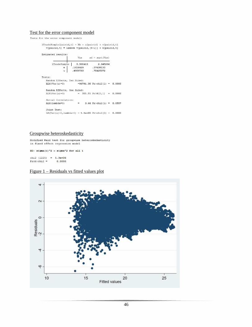
46

Test for the error component model

Groupwise heteroskedasticity

Figure 1 – Residuals vs fitted values plot

47

TESTS FOR NORMALITY

Normal data test developed by Shapiro-Wilk

Variable Obs W V z Prob>z

residual 27,234 0.812 2167.108 21.060 0.000

Table 3 - tests for Normality shown by Kurtosis / Skewness Variable Obser Pr(Skewness) Pr(Kurtosis) adj_chi2(2) Prob>chi2

Log of aggr.

exports 31,098 0 0 . 0

Exporter’s GDP 31,079 0 0.001 69.08 0

Importer’s GDP 31,078 0 0.001 70.25 0

Distance 31,098 0 0 . .

Contiguity 31,098 0 0 . .

Common lang. 31,098 0 0 . .

Colony post-45 31,098 0 0 . .

Common col. 31,098 0 0 . .

Same country 31,098 0 0 . .

RTA 31,098 0 . . .

EU 31,079 0 0 . .

Common Cur. 31,098 0 0 . .

FDI stock in. 31,098 0 0 . .

FDI stock out. 31,098 0 0 . .

Governmnt size 29,098 0 0 . .

Market Open. 31,098 0 0 . .

Econ. Glob. 29,802 0 0 . .

Polit. Glob. 29,802 0 0 . .

Rule of law 31,098 0 0 . .

Internet &

mobile 30,684 0 0 . .

Air transport 31,098 0 0 . .

Total Infrastructure

Investment

31,079 0 0 . .

Importer’s MFN tariffs

30,523 0 0 . .

Political

Stability 31,098 0 0 . .

48

Figure 2: Histogram of the residuals with overlay normal curve

AUTOCORRELATION

Figure 3: Autocorrelation of the residuals over the period 1995-2018 for United States of America (USA)

with importing partner countries.

49

Regression of residuals on one period lagged residual with pair and time fixed effects and disturbances

clustered by the pair of countries

(1)

uhat

l1.uhat 0.586***

(0.0188)

_cons -0.0172*

(0.00680)

N 24853

Fixed effects Country-time, Pair

Standard errors in parentheses, other covariates used in the main table are regressed but not displayed, to

save space. * p < 0.05, ** p < 0.01, *** p < 0.001

Wooldridge test on first order autocorrelation

Table 4: The Breusch-Godfrey test

(1)

uhat

One period lagged residuals 0.570*** (0.0261)

Two period lagged residuals 0.0930*** (0.0212)

_cons 4.075*** (0.950)

Number of observations 23366

R-squared 0.431 Disturbances in parentheses * p < 0.05, ** p < 0.01, *** p < 0.001. Other covariates employed in the main table are regressed but not displayed for

conciseness

50

MULTICOLLINEARITY

TABLE 5 - VIF

Variance inflation factor

VIF

Exporter’s GDP 4.849

Rule of law 3.937

Distance 3.876

Political globalization 3.572

Economic globalization 3.425

Market openness 2.857

Political stability 2.537

FDI stock inward 2.535

EU 2.399

FDI stock outward 2.234

RTA 2.208

Fixed telephone subs. 2.208

Internet and mobile subs. 2.175

Air transport freight 2.057

Government size 2.045

Total infrastructure investment 1.701

Importer’s GDP 1.666

Contiguity 1.615

Common currency 1.499

Importer’s MFN tariffs 1.498

Same country 1.295

Common official language 1.289

Colony 1.205

Common colony 1.131

Mean VIF 2.326

51

TABLE 6 – CORRELATION MATRIX

Log of aggr.

exports Exporter’s

GDP Importer’s

GDP Distance Contiguity

Common

language Colony post-

45 Common

colonizer Same

country RTA EU

Common

Cur. FDI stock in.

FDI stock

out.

Log of aggr. exports 1.00

Exporter’s GDP 0.53 1.00

Importer’s GDP 0.51 0.05 1.00

Distance -0.47 0.09 0.09 1.00

Contiguity 0.43 0.03 0.03 -0.64 1.00

Common language 0.35 0.10 0.10 -0.39 0.46 1.00

Colony post-45 0.35 0.05 0.05 -0.53 0.50 0.57 1.00

Common colonizer 0.33 -0.05 -0.05 -0.74 0.56 0.48 0.60 1.00

Same country 0.32 -0.05 -0.06 -0.70 0.64 0.41 0.59 0.70 1.00

RTA 0.20 -0.13 -0.14 -0.53 0.21 0.02 0.04 0.12 0.15 1.00

EU 0.28 0.02 0.02 -0.37 0.14 -0.06 -0.02 0.01 0.07 0.44 1.00

Common Cur. 0.33 0.05 0.04 -0.49 0.34 0.23 0.25 0.40 0.35 0.26 0.48 1.00

FDI stock in. 0.57 0.40 0.41 -0.06 0.13 0.12 0.05 -0.10 -0.07 0.07 0.24 0.12 1.00 FDI stock out. 0.58 0.51 0.31 -0.06 0.13 0.11 0.05 -0.10 -0.06 0.07 0.22 0.11 0.64 1.00

Rule of law 0.16 0.21 0.03 0.01 0.01 0.05 0.02 -0.01 -0.02 -0.03 0.04 0.04 0.18 0.24

Internet & mobile 0.23 0.22 0.17 -0.02 0.00 0.01 0.00 0.00 -0.01 0.15 0.22 0.15 0.28 0.29

Fixed telephone subs 0.19 0.26 -0.05 -0.04 0.02 0.07 0.03 -0.02 -0.03 -0.06 0.02 0.03 0.19 0.34

Air transport 0.21 0.54 -0.03 0.16 -0.01 0.12 0.03 -0.03 -0.06 -0.20 -0.15 0.01 0.14 0.19

Total infrast. Invest. 0.20 0.21 0.01 -0.12 0.07 -0.01 0.02 0.00 0.01 0.04 0.14 0.04 0.20 0.27

Importer’s MFN tariff -0.19 -0.11 -0.08 0.16 -0.05 0.00 -0.01 -0.01 -0.03 -0.18 -0.31 -0.19 -0.25 -0.17

Political Stability 0.10 -0.05 -0.02 -0.11 0.05 -0.02 -0.01 0.01 0.04 0.05 0.15 0.06 0.12 0.18

Rule of law Internet &

mobile

Fixed telephone

subs Air transport

Total infrast.

Invest Importer’s

MFN tariff Political

Stability

Rule of law 1.00

Internet & mobile 0.30 1.00

Fixed telephone subs 0.24 0.14 1.00

Air transport 0.08 -0.06 0.29 1.00

Total infrast. Invest 0.18 0.24 0.35 -0.11 1.00

Importer’s MFN tariff -0.15 -0.52 0.08 0.07 -0.05 1.00

Political Stability 0.25 0.16 0.39 -0.16 0.48 0.04 1.00

52

Random effects vs Fixed effects

Lagrangian Multiplier test

Sargan-Hansen - Test of overidentifying restrictions

By using the -xtoverid- command, which applies the approach of artificial regression demonstrated by

Arellano (1993) and Wooldridge (2002, pp 290-91), in which a random effects model is re-estimated,

supplemented with additional variables converted into deviations-from-mean form comprising the original

regressors. Rejection means that, unlike the Hausman test, the fixed effect model is chosen, This test extends

itself to heteroskedastic and clustered robust alternatives.

Likelihood-ratio test of no fixed-effects vs individual, and time fixed effects

Likelihood-ratio test where m2 represents no fixed effects vs m3 with time and pair FE

53

C: RESIDUALS VS FITTED VALUES, FITTED VALUES VS THE DEPENDENT VARIABLE AND RESET TEST

MAIN TABLE:

Column 1

Reset test Column 1:

Column 2

Reset test Column 2:

54

D: RESULTS AND DISCUSSION

FIGURE 4: KERNEL DENSITY FOR THE MAIN TABLE

FIGURE 5: KERNEL DENSITY FOR THE ROBUSTNESS TABLE

55

Table 7: Descriptive statistics for the robustness table

Variables N Mean Standard

Deviations

Minimum Maximum Skewness Kurtosis

Investment freedom 31098 4.213 .527 0 4.554 -7.079 56.677

Trade freedom 31098 4.335 .522 0 4.5 -7.97 66.272

Financial freedom 31098 4.141 .542 0 4.5 -6.203 47.469

Economic

globalization

29802 1.849 .078 1.531 1.963 -1.237 4.422

Political globalization 29802 1.928 .065 1.626 1.994 -1.622 5.612

Rule of law 31098 0 1 -7.347 .699 -5.531 40.62

Port infrastructure

quality

16812 .693 .084 .418 .833 -.814 3.172

Road Infrastructure

quality

16848 .684 .099 .281 .827 -1.031 3.946

Rail Infrastructure

quality

12600 .621 .137 .146 .833 -.957 4.166

Air Infrastructure

quality

16812 .729 .068 .502 .827 -1.106 3.649

Importer’s tariffs

(MFN)

30523 1.615 .331 .916 2.878 1.482 4.808

Fragile state index 1 15552 0 1 -3.113 2.307 -.195 3.589

Fragile state index 2 15552 0 1 -2.527 2.028 -.199 2.11

Innovation index 10332 1.698 .075 1.484 1.835 -.576 2.531

56

E: DIAGNOSTICS FOR ROBUSTNESS TABLE

HETEROSKEDASTICITY

Heteroskedasticity test by Cook-Weisberg / Breusch-Pagan of fitted values Null Hypothesis: Variance that is constant Variable: log of aggregate exports fitted values

Chi-square = 432.32

Prob > chi2 = 0.0000

Heteroskedasticity test by Cook-Weisberg / Breusch-Pagan of fitted values Null Hypothesis: Variance that is constant Variables: lEXP_gdp lIMP_gdp ldistw contig comlang_off colony comcol smctry rta eu comcur

PCAGovSize lEXP_InvestFreedom lEXP_TradeFreedom lEXP_FinanFreedom EXP_EconGlobalization

EXP_PoliticalGlobal PCARuleOfLaw lEXP_QualityofPortInfras lEXP_QualityofRoadInfras

lEXP_QualityofRailInfras lEXP_QualityofAirInfras lIMP_TariffMFN EXP_FRAGILE1

EXP_FRAGILE2

lEXP_InnovationIndex

F(26 , 7960) = 39.01

Prob > F = 0.0000

Test developed by white, where the null hypothesis is Homoskedasticity

Alternative hypothesis: unrestricted heteroskedasticity

Chi-square (358) = 1990.10

Probability to have higher than Chi-square = 0.0000

Cameron & Trivedi's IM-test decomposition

Source chi2 df p

Heteroscedasticity 1990.100 358 0.000

Curve Skewness 143.680 26 0.000

Curve Kurtosis 26.090 1 0.000

The Total 2159.860 385 0.000

57

Figure 6: Residuals plot

Tests for the error component model:

Estimated results:

Var sd = sqrt(Var)

lTradeSimple 4.580 2.140

e 0.053 0.231

u 0.535 0.732

Tests:

Random Effects, Two Sided:

ALM(Var(u)=0) =12512.27 Pr>chi2(1) = 0.0000

Random Effects, One Sided:

ALM(Var(u)=0) = 111.86 Pr>N(0,1) = 0.0000

Serial Correlation:

ALM(lambda=0) = 7.94 Pr>chi2(1) = 0.0048

Joint Test:

LM(Var(u)=0,lambda=0) =18240.70 Pr>chi2(2) = 0.0000

58

NORMALITY TESTS

Shapiro-Wilk W test for normal data

Table 3 - tests for Normality shown by Kurtosis / Skewness Variable Obs Pr(Skewness) Pr(Kurtosis) adj chi2(2) Prob>chi2

Log of

aggregate

exports 30,234 0 0 . 0

Exporter’s GDP 30,234 0 0.0012 67.38 0

Importer’s

GDP 30,234 0 0.0014 68.34 0

Distance 30,234 0 0 . .

Contiguity 30,234 0 0 . .

Common lang. 30,234 0 0 . .

Colonial link 30,234 0 0 . .

Common col. 30,234 0 0 . .

Same country 30,234 0 0 . .

RTA 30,234 0 . . .

EU 30,234 0 0 . .

Common

Currency 30,234 0 0 . .

Government size 28,309 0 0 . .

Investment

freedom 30,234 0 0 . .

Trade freedom 30,234 0 0 . .

Financial freedom 30,234 0 0 . .

Economic

globalization 28,974 0 0 . .

Political globalization 28,974 0 0 . .

Rule of law 30,234 0 0 . .

Quality of port

infrastructure 16,345 0 0 . .

Quality of road infrastructure 16,380 0 0 . .

Quality of rail

infrastructure 12,250 0 0 . .

Quality of air infrastructure 16,345 0 0 . .

Importer’s

MFN tariffs 29,675 0 0 . .

Fragile state index 1 15,120 0 0 . 0

Fragile state

index 2 15,120 0 0 . .

Innovation index 10,045 0 0 . 0

Shapiro-Francia W' test for normal data

Variable Obs W' V' z Prob>z

residual 7,987 0.997 14.496 6.968 0.000

Note: The normal approximation to the sampling distribution of W'

is valid for 10<=n<=5000 under the log transformation.

59

Figure 7: Histogram of the residuals with overlay normal curve

60

AUTOCORRELATION

Panel data: Autocorrelation test by Wooldridge

Null Hypothesis: No autocorrelation of the first order

F(1, 1218) = 81.499

Prob > F = 0.000

Test of Breusch Godfrey

Regression of the lagged residuals of first and second order on the residual indicates significant impact of

the lagged residuals.

(1) uhat

l1uhat 0.767*** (0.029)

l2uhat 0.179*** (0.028)

N 5512

R-squared 0.954

Standard errors in

parentheses

Note: only lagged residuals

are displayed

Chi square multiplier lagrange statistic calculation = 5512* 0.954=5258.44, the test rejects the null and we

find that we do have significant autocorrelation.

61

MULTICOLLINEARITY TESTS

VIF

Table 9: Variance inflation factor for Robustness Table

VIF

Rule of law 7.499

Exporter’s innovation index 6.975

Exporter’s economic globalization 6.167

Exporter’s Fragile state index 2 5.428

Exporter’s quality of railroad infrastructure 4.827

Exporter’s GDP 4.823

Distance 4.141

Exporter’s political globalization 3.947

Exporter’s quality of road infrastructure 3.643

EU 3.38

Exporter’s air transport infrastructure quality 2.998

Exporter’s port infrastructure quality 2.977

Exporter’s investment freedom 2.536

RTA 2.508

Exporter’s Fragile state index 1 2.4

Exporter’s Government size 2.282

Exporter’s Trade freedom 2.146

Exporter’s Financial freedom 1.992

Common Currency 1.695

Contiguity 1.628

Importer’s MFN tariffs 1.416

Common official language 1.311

Same country in the past 1.305

Colonial link 1.216

Importer’s GDP 1.158

Common colonizer post-1945 1.139

Mean VIF 3.136

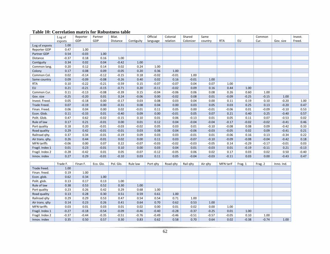
62

Table 10: Correlation matrix for Robustness table

Log of exports

Reporter GDP

Partner GDP

Bilat. Distance Contiguity

Official language

Colonial relation

Shared Colonizer

Same country RTA EU

Common Cur. Gov. size

Invest. Freed.

Log of exports 1.00 Reporter GDP 0.47 1.00 Partner GDP 0.54 -0.03 1.00 Distance -0.37 0.18 0.16 1.00 Contiguity 0.34 0.02 0.04 -0.42 1.00 Common lang. 0.20 0.12 0.14 0.02 0.24 1.00 Colony 0.17 0.08 0.09 -0.05 0.20 0.36 1.00 Common Col. 0.02 -0.14 -0.12 -0.15 0.18 -0.02 -0.01 1.00 Same country 0.09 -0.09 -0.08 -0.26 0.40 0.02 0.16 -0.01 1.00 RTA 0.10 -0.22 -0.21 -0.59 0.15 -0.07 -0.07 0.04 0.07 1.00 EU 0.21 -0.21 -0.15 -0.71 0.20 -0.11 -0.02 0.09 0.16 0.44 1.00 Common Cur. 0.11 -0.13 -0.08 -0.39 0.15 -0.04 -0.06 0.06 0.08 0.26 0.60 1.00 Gov. size -0.25 -0.20 0.01 0.24 -0.06 0.00 -0.02 0.08 0.01 -0.09 -0.25 -0.15 1.00 Invest. Freed. 0.05 -0.18 0.00 -0.17 0.03 0.08 0.03 0.04 0.00 0.11 0.19 0.10 -0.20 1.00

Trade Freed. 0.07 -0.19 0.00 -0.31 0.08 0.04 0.00 0.03 0.05 0.03 0.25 0.13 -0.20 0.47

Finan. Freed. 0.06 0.04 0.00 0.02 -0.01 0.11 0.05 0.00 -0.01 -0.06 0.01 -0.09 -0.10 0.53

Econ. Glob. 0.11 -0.33 0.01 -0.40 0.09 0.00 -0.01 0.05 0.07 0.21 0.40 0.25 -0.40 0.57

Polit. Glob. 0.47 0.62 -0.02 -0.15 0.10 0.01 0.06 -0.13 0.01 0.05 0.11 0.07 -0.53 0.02

Rule of law 0.17 0.21 -0.01 0.00 0.01 0.12 0.04 -0.04 -0.04 -0.17 -0.02 -0.02 -0.41 0.46

Port quality 0.18 0.20 -0.01 -0.03 -0.02 0.05 0.03 0.01 -0.10 -0.08 0.08 0.09 -0.42 0.33

Road quality 0.29 0.42 -0.01 -0.01 0.03 0.08 0.04 -0.06 -0.03 -0.05 0.02 0.09 -0.41 0.21

Railroad qlty. 0.37 0.34 -0.01 -0.19 0.09 0.03 0.03 -0.01 0.01 -0.06 0.16 0.13 -0.34 0.22

Air trans. qlty. 0.26 0.44 -0.01 0.02 0.00 0.11 0.03 -0.07 -0.10 -0.09 -0.08 -0.04 -0.42 0.18

MFN tariffs -0.06 0.00 0.07 0.22 -0.07 -0.03 -0.02 -0.03 -0.05 0.14 -0.29 -0.17 -0.01 0.03

Fragil. Index 1 0.01 0.23 -0.01 0.10 0.00 0.03 0.04 0.01 -0.03 0.01 -0.19 -0.11 0.21 -0.13

Fragil. Index 2 -0.28 -0.42 0.01 0.05 -0.07 -0.12 -0.05 0.06 0.02 0.17 0.03 0.02 0.50 -0.40

Innov. index 0.27 0.29 -0.01 -0.10 0.03 0.11 0.05 -0.04 -0.03 -0.11 0.03 0.00 -0.43 0.47

Trade F. Finan F. Eco. Glo. Pol. Glo. Rule law Port qlty Road qlty Rail qlty Air qlty MFN tarif Frag. 1 Frag. 2 Inno. Ind. Trade freed. 1.00 Finan. freed. 0.19 1.00 Econ. glob. 0.62 0.34 1.00 Polit. glob. 0.13 0.17 0.13 1.00 Rule of law 0.38 0.53 0.52 0.30 1.00 Port quality 0.23 0.26 0.42 0.29 0.68 1.00 Road quality 0.13 0.28 0.30 0.51 0.59 0.61 1.00 Railroad qlty 0.29 0.29 0.53 0.47 0.54 0.54 0.71 1.00 Air trans. qlty 0.14 0.23 0.26 0.41 0.64 0.70 0.62 0.53 1.00 MFN tariffs 0.03 0.01 0.03 0.01 0.02 0.00 0.01 0.02 0.00 1.00 Fragil. Index 1 -0.27 -0.18 -0.54 -0.09 -0.46 -0.40 -0.28 -0.37 -0.25 0.01 1.00 Fragil. Index 2 -0.37 -0.44 -0.35 -0.51 -0.76 -0.49 -0.46 -0.51 -0.57 -0.05 0.10 1.00 Innov. index 0.35 0.50 0.57 0.30 0.83 0.62 0.58 0.70 0.64 0.02 -0.38 -0.74 1.00

63

Random effects vs Fixed effects

Lagrangian multiplier test

Sargan-Hansen – Overidentifying restrictions test

Likelihood-ratio test of no fixed-effects vs individual, and time fixed effects

Likelihood-ratio test where m2 represents no fixed effects vs m3 with time and pair FE

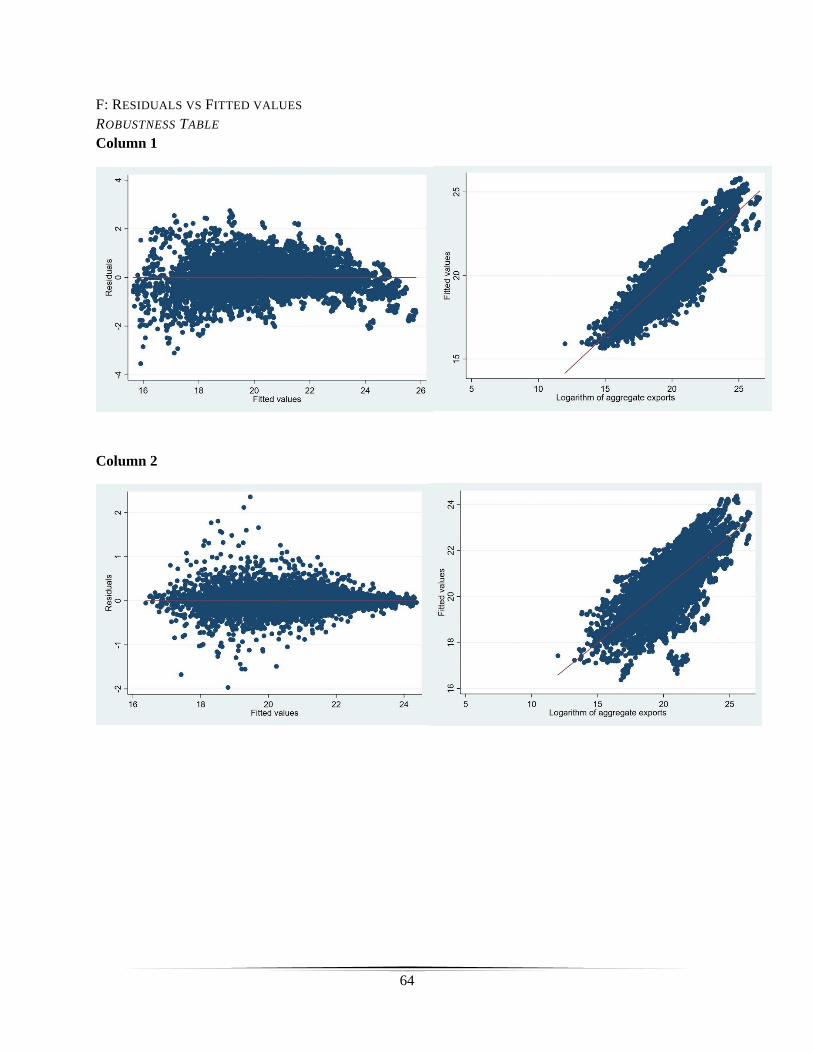
64

F: RESIDUALS VS FITTED VALUES

ROBUSTNESS TABLE

Column 1

Column 2

65

G: THEORETICAL FOUNDATIONS OF GRAVITY MODEL

Figure 8

H: TRADITIONAL SPECIFICATIONS

The econometric theory lays down three sufficient and necessary conditions for OLS

1. The error 𝜀𝑖𝑗𝑡 must be uncorrelated with each of the independent variables and have mean equal to

zero.

2. The disturbances 𝜀𝑖𝑗𝑡 ought to be drawn independently from a distribution that is normal with a

given variance.

3. The explanatory variables must not be a linear combination of other independent variables

66

The basic gravity model of internation trade flows

Table 11:

--------------------------------------------------------------

(1) (2) (3) (4) Log of AVG Trade Average of Log of SUM Sum of logs Logs of trade of trade of trade

--------------------------------------------------------------

Exp_GDP 0.368*** 0.316*** 0.883*** 5773.3***

(0.003) (0.002) (0.003) (26.049)

Imp_GDP 0.570*** 0.323*** 0.850*** 3105.2***

(0.003) (0.002) (0.003) (26.038)

Distance -0.377*** -0.359*** -1.001*** -6398.7***

(0.004) (0.003) (0.005) (42.274)

contiguity 0.638*** 0.826*** 0.360*** 10663.8***

(0.021) (0.015) (0.026) (208.868)

Language 0.237*** 0.208*** 0.521*** 4267.4***

(0.019) (0.013) (0.023) (186.691)

colony -0.0268 -0.0617*** 0.209*** 2369.7***

(0.025) (0.018) (0.031) (252.015)

comcol 0.661*** 0.196*** 2.558*** 10642.2***

(0.063) (0.045) (0.077) (629.865)

_cons -8.641*** -3.554*** -17.84*** -167210.0***

(0.098) (0.070) (0.120) (971.547)

--------------------------------------------------------------

N 30234 30234 30234 30234

R-sq 0.723 0.733 0.857 0.767

--------------------------------------------------------------

In parentheses standard errors are displayed

* p-value<0.1, ** p-value <0.05, *** p-value<0.01

The regression with the logarithms of the average trade is shown in Column 1. Column 2 depicts the

regression (the theoretically correct method) with the average of the logarithms. The regression of the

aggregated bilateral trade flows is shown in Column 3. Column 4 is the regression with the aggregated logs

of bilateral trade flows.

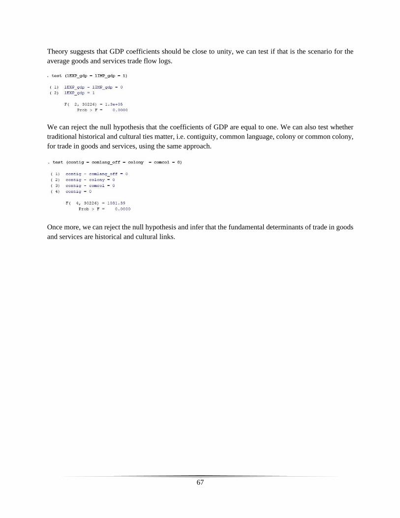
67

Theory suggests that GDP coefficients should be close to unity, we can test if that is the scenario for the

average goods and services trade flow logs.

We can reject the null hypothesis that the coefficients of GDP are equal to one. We can also test whether

traditional historical and cultural ties matter, i.e. contiguity, common language, colony or common colony,

for trade in goods and services, using the same approach.

Once more, we can reject the null hypothesis and infer that the fundamental determinants of trade in goods

and services are historical and cultural links.

68

I: VARIABLE INFORMATION

CONSTRUCTED INDEXES:

Figure 9: Interpolation of political stability for years 1997, 1999 and 2001

69

PRINCIPAL COMPONENT ANALYSIS FOR INSTITUTIONS, GLOBALIZATION AND INFRASTRUCTURE

Matrix of correlations

Variables (1) (2) (3) (4) (5) (6) (7) (8) (9) (10) (11)

(1) Property rights 1.000

(2) Freedom from Corr. 0.841 1.000

(3) Tax burden -0.342 -0.356 1.000

(4) Gov. spending -0.211 -0.314 0.639 1.000

(5) Fiscal freedom -0.349 -0.363 0.990 0.618 1.000

(6) Trade freedom 0.250 0.331 0.046 -0.108 0.055 1.000

(7) Investment freedom 0.360 0.266 -0.035 -0.102 -0.020 0.408 1.000

(8) Financial freedom 0.396 0.367 -0.017 -0.042 0.013 0.223 0.422 1.000

(9) Economic global. 0.442 0.500 -0.250 -0.363 -0.221 0.576 0.499 0.403 1.000

(10) Political global. 0.351 0.347 -0.428 -0.327 -0.438 0.303 0.064 0.143 0.281 1.000

(11) Social global. 0.563 0.674 -0.187 -0.316 -0.185 0.646 0.359 0.386 0.744 0.386 1.000

PCARuleOfLaw: This index incorporates the property rights index with freedom from corruption

index

70

PCAGovSize: Represents the government size index, composed of the tax burden, government

spending and fiscal freedom indexes.

71

PCAMarketOpeness: stands for the market openness index composed of trade, financial and

investment freedom.

72

PCAGlobalization: Globalization index is composed of economic, political and social globalization

indexes

73

PCAInternetMobileSubs: Represents an index of internet and mobile subscriptions

74

PCA construction for Fragile State Index:

Matrix of correlations

Variables (1) (2) (3) (4) (5) (6) (7) (8) (9) (10) (11)

(1) Security threats 1.000

(2) Factionalized elites 0.750 1.000

(3) Group grievance 0.680 0.700 1.000

(4) Economic decline 0.507 0.509 0.355 1.000

(5) Uneven econ. dev. 0.607 0.609 0.637 0.448 1.000

(6) Brain drain 0.542 0.523 0.338 0.552 0.489 1.000

(7) State legitimacy 0.698 0.788 0.570 0.641 0.744 0.726 1.000

(8) Public services 0.738 0.672 0.513 0.658 0.751 0.712 0.835 1.000

(9) Human rights 0.695 0.641 0.577 0.459 0.767 0.603 0.815 0.827 1.000

(10)Demograp.

pressure

0.622 0.538 0.552 0.336 0.705 0.542 0.657 0.755 0.781 1.000

(11) Refugees 0.632 0.666 0.594 0.226 0.481 0.410 0.587 0.507 0.570 0.571 1.000

Factor correlation/analysis Number of obser. = 15,552

Method: principal-component factors Retained factors = 2

Rotation: (unrotated) Number of params = 21

Factor Eigenvalue Difference Proportion Cumulative

Factor1 7.153 6.106 0.650 0.650

Factor2 1.047 0.313 0.095 0.745

Factor3 0.733 0.173 0.067 0.812

Factor4 0.561 0.225 0.051 0.863

Factor5 0.335 0.019 0.030 0.893

Factor6 0.316 0.039 0.029 0.922

Factor7 0.278 0.075 0.025 0.948

Factor8 0.203 0.021 0.018 0.966

Factor9 0.182 0.077 0.017 0.983

Factor10 0.105 0.018 0.010 0.992

Factor11 0.087 . 0.008 1.000

Factor loadings (pattern matrix) and unique variances

Variable Factor1 Factor2 Uniqueness

Security threats 0.847 -0.138 0.264

Factionalized elites 0.838 -0.168 0.270

Group grievance 0.734 -0.434 0.273

Economic decline 0.635 0.558 0.285

Uneven econ. dev 0.825 -0.047 0.317

Brain drain 0.726 0.418 0.298

State legitimacy 0.916 0.166 0.133

Public services 0.907 0.246 0.118

Human rights 0.884 0.004 0.219

Demograph. pressure 0.804 -0.113 0.340

Refugees 0.703 -0.471 0.284

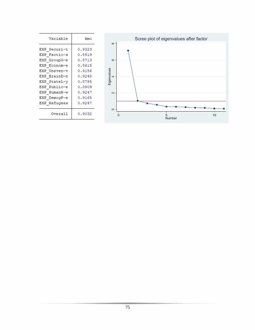
75