UEA Insurance Stats Overview Steve Cant Senior Statistics Manager, Aviva steve.cant @ aviva.co.uk...
21
UEA Insurance Stats Overview Steve Cant Senior Statistics Manager, Aviva steve.cant @ aviva.co.uk 01603 686857
-
date post
19-Dec-2015 -
Category
Documents
-
view
213 -
download
0
Transcript of UEA Insurance Stats Overview Steve Cant Senior Statistics Manager, Aviva steve.cant @ aviva.co.uk...
UEAInsurance Stats Overview
Steve Cant
Senior Statistics Manager, Aviva
steve.cant @ aviva.co.uk01603 686857

Modelling Opportunities at AvivaDoes modelling risk have any appeal ?Are you interested in an actuarial career but don’t fancy years more study in your free time ?Do you have graduate level maths skills ?Do you have any idea what financial statisticians do ? Have you ever wondered how insurance premiums are calculated ?
Key Aspects of RoleBuilding risk cost models – to predict who will claim on their motor or household insuranceBehavioural modelling – to predict how customers will react to pricing decisionsSpatial analysis of postcode area in order to produce world leading maps of insurance riskExtraction of deeper knowledge from large, already well understood data setsR & D into new modelling and analytical techniquesEducated guessworkWorking with colleagues across the business including those in pricing, marketing, finance, actuarial, claims and underwriting
You’ll apply your analytical enthusiasm to a range of business problems and produce mathematical and statistical models that drive real results.
The Elusive Advert - extracts

Products (Personal)
Motor
Household
Bike Van
Pet Travel
CreditorBreakdown
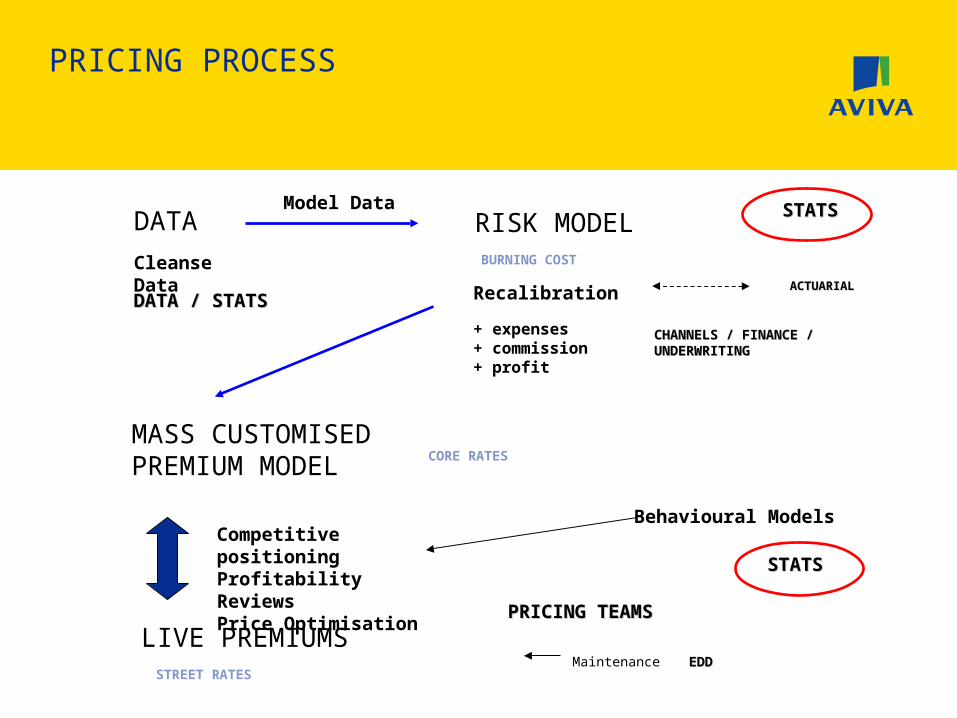
PRICING PROCESS
DATA RISK MODEL
MASS CUSTOMISEDPREMIUM MODEL
LIVE PREMIUMS
Cleanse Data
Recalibration
Competitive positioningProfitability ReviewsPrice Optimisation
DATA / STATS DATA / STATS
STATSSTATS
PRICING TEAMSPRICING TEAMS
Model Data
CHANNELS / FINANCE / CHANNELS / FINANCE / UNDERWRITINGUNDERWRITING
ACTUARIALACTUARIAL
Behavioural Models
STATSSTATS
BURNING COST
+ expenses + commission + profit
STREET RATES Maintenance EDDEDD
CORE RATES

AM80 and AF80 2 years select q[x-t]+t
0.000000
0.000500
0.001000
0.001500
0.002000
0.002500
0.003000
0.003500
0.004000
0.004500
0 2 4 6 8 10 12 14 16 18 20 22 24 26 28 30 32 34 36 38 40 42 44 46 48 50
Death
Age

0.0
1.0
2.0
3.0
4.0
5.0
6.0
7.0
8.0
Main Driver Age
Rela
tive F
req
uen
cy
FE
MA
Large Bodily Injury Claims – Major crashesTHIRD PARTY ONLY
10 years of data > £250K frequencyStill overwhelmingly random and rare – but can produce an index
About 1 in 5000 vehicle years
About 1 in 40000 vehicle years
Anything that influences risk is a rating factor

MOTOR RISK COST MODEL – Ranked by Information Gain
1 Bodily Injury Freq District 14 Property Damage Freq District
2 Young Additional Driver Age 15 Own Damage District
3 NCD 16 Vehicle Age
4 Main Driver Age 17 Transmission
5 Young Additional Driver Sex 18 Theft Freq District
6 Car Group 19 Fuel Type
7 Ritz 20 Duration
8 Driving Restriction 21 Convictions
9 Payment Frequency 22 Licence Length
10 Make Model 23 YAD Owns Car
11 Ownership Length 24 PNCD
12 Mileage 25 Voluntary Excess
13 At Fault Claims etc 30 other factors
Motor Insurance Rating Factors
Information gain is a weighted combination of factor range and exposure. E.g. age has high loadings for low exposure, payment method has lower loadings on high exposure.
Postcode
Vehicle

Insurance Premiums
Start with a base (average) premium E.g. £400 (40 year old, 3 year old Ford Focus in Norwich, with full No Claims)Then add various loadings and discounts
18 year old driver 200% loadingLives in Liverpool 100% loadingDrives a small car 40% discountDrives an old car 30% discountNo Claims Discount is zero 233% loading ! (5 years No Claims is a 70% discount)
£400 x 3 = £1200 x 2 = £2400x 0.6 = £1440x 0.7 = £1008x 3.33 = £3360 !
Harsh ?
How do we calculate these loadings ?

CHAOS
The Claims Universe
Undiscovered OrderNew factorsImproved modelling
ORDER
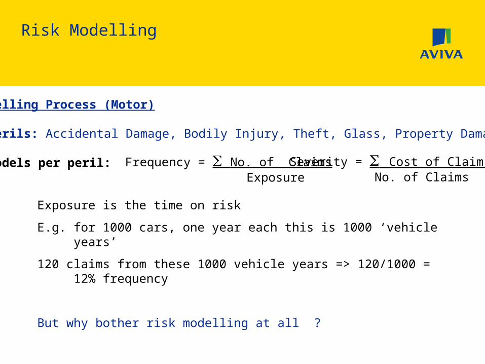
Modelling Process (Motor)
5 Perils: Accidental Damage, Bodily Injury, Theft, Glass, Property Damage 2 Models per peril:
Risk Modelling
Frequency = No. of Claims Exposure
Severity = Cost of Claim No. of Claims
Exposure is the time on risk
E.g. for 1000 cars, one year each this is 1000 ‘vehicle years’
120 claims from these 1000 vehicle years => 120/1000 = 12% frequency
But why bother risk modelling at all ?
Attempt to remove random effects (noise)
Avoid the illusions of variable association (Simpson’s paradox)
Consider all rating factors ‘together’ in order to discover ‘true effect’
Examine consistency over time
Ensure best possible prediction of future risk
Multivariate Modelling
Why bother ?
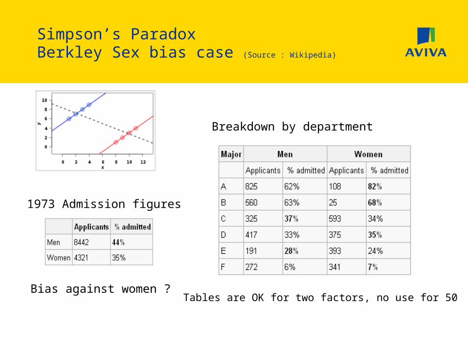
Simpson’s ParadoxBerkley Sex bias case (Source : Wikipedia)
Bias against women ?
1973 Admission figures
Breakdown by department
Tables are OK for two factors, no use for 50
Linear Modelling
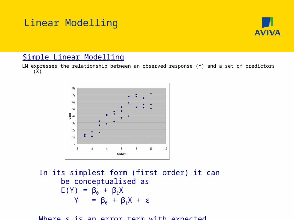
LM expresses the relationship between an observed response (Y) and a set of predictors (X)
In its simplest form (first order) it can be conceptualised asE(Y) = β0 + β1X Y = β0 + β1X + ε
Where ε is an error term with expected value of 0
0
10
20
30
40
50
60
70
80
0 2 4 6 8 10 12
District
Cos
t
Simple Linear Modelling
Linear Modelling
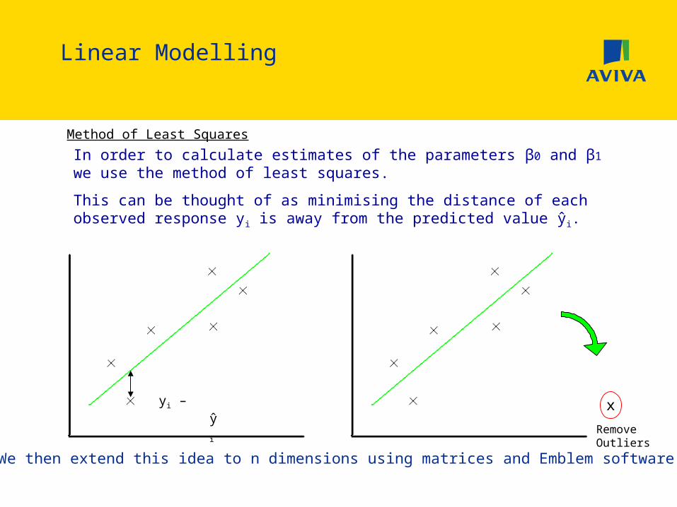
Method of Least Squares
In order to calculate estimates of the parameters β0 and β1 we use the method of least squares.
This can be thought of as minimising the distance of each observed response y i is away from the predicted value ŷi.
yi – ŷi
x
Remove Outliers
We then extend this idea to n dimensions using matrices and Emblem software

Linear Modelling
Method of Least Squares
Minimize the Sum of Squared Errors;
By differentiating it can be shown that to minimise the SSE we must solve the following;
Linear Modelling
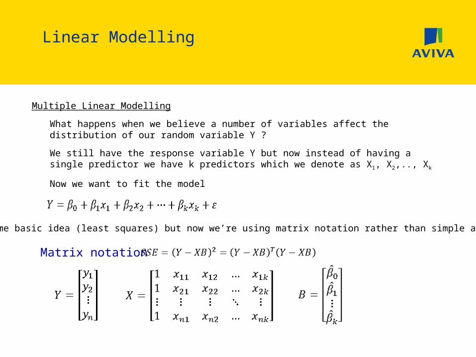
Multiple Linear Modelling
What happens when we believe a number of variables affect the distribution of our random variable Y ?
We still have the response variable Y but now instead of having a single predictor we have k predictors which we denote as X1, X2,.., Xk
Now we want to fit the model
So the same basic idea (least squares) but now we’re using matrix notation rather than simple algebra
Matrix notation

Generalized Linear Model (GLM)
Normal Distribution
• assumes each observation has the same fixed variance (no tail)
Poisson Distribution
• assumes the variance increases with the expected value of each observation (longer tail)
Gamma Distribution
• assumes variance increases with the square of the expected value (even longer tail !)
Basically An extension of Linear modelling that allows
Multiplicative models (using a ‘link function’) - more appropriate for insurance
A wider selection of errors (‘loss distributions’) from the exponential family

Emblem Software
• Raw data alone can lead to the wrong conclusion

Base 42% in Ritz 7-10
Age 50 +
Annual payers
Better Wealth Postcode
Policy Duration 3+
76% in Ritz 7-10Exposure 9%
73% in Ritz 7-10Exposure 17%
Ritz 7-10 SegmentationNUD (NB & Renewals)
67% in Ritz 7-10Exposure 27%
Proportion Ritz 1- 6
Proportion Ritz 7- 10
Data Mining
Decision Trees – Visual carve up of account

District – a quantum change in quality
2005 2010 X 10 Perils

© Aviva plc
THE END
Any questions ?