UE SPECTRALYZER

INSTRUCTION MANUAL

14 Hayes Street Elmsford, NY 10523

PH: 914-592-1220 Fax: 914-347-2181

Email: info@uesystems.com V 4.2

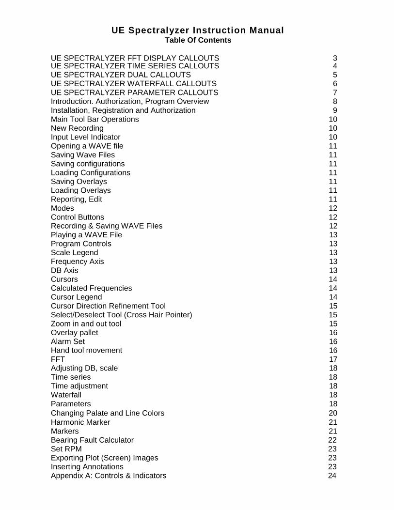
UE Spectralyzer Instruction Manual Table Of Contents

UE SPECTRALYZER FFT DISPLAY CALLOUTS 3 UE SPECTRALYZER TIME SERIES CALLOUTS 4 UE SPECTRALYZER DUAL CALLOUTS 5 UE SPECTRALYZER WATERFALL CALLOUTS 6 UE SPECTRALYZER PARAMETER CALLOUTS 7 Introduction. Authorization, Program Overview 8 Installation, Registration and Authorization 9 Main Tool Bar Operations 10 New Recording 10 Input Level Indicator 10 Opening a WAVE file 11 Saving Wave Files 11 Saving configurations 11 Loading Configurations 11 Saving Overlays 11 Loading Overlays 11 Reporting, Edit 11 Modes 12 Control Buttons 12 Recording & Saving WAVE Files 12 Playing a WAVE File 13 Program Controls 13 Scale Legend 13 Frequency Axis 13 DB Axis 13 Cursors 14 Calculated Frequencies 14 Cursor Legend 14 Cursor Direction Refinement Tool 15 Select/Deselect Tool (Cross Hair Pointer) 15 Zoom in and out tool 15 Overlay pallet 16 Alarm Set 16 Hand tool movement 16 FFT 17 Adjusting DB, scale 18 Time series 18 Time adjustment 18 Waterfall 18 Parameters 18

Changing Palate and Line Colors 20

Harmonic Marker 21 Markers 21 Bearing Fault Calculator 22 Set RPM 23 Exporting Plot (Screen) Images 23 Inserting Annotations 23 Appendix A: Controls & Indicators 24

3

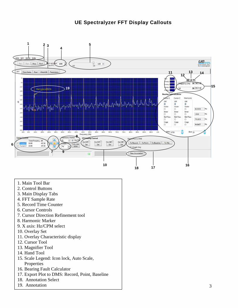
UE Spectralyzer FFT Display Callouts

1 3 2

1. Main Tool Bar

2. Control Buttons

3. Main Display Tabs

4. FFT Sample Rate

5. Record Time Counter

6. Cursor Controls

7. Cursor Direction Refinement tool

8. Harmonic Marker

9. X axis: Hz/CPM select

10. Overlay Set

11. Overlay Characteristic display

12. Cursor Tool

13. Magnifier Tool

14. Hand Tool

15. Scale Legend: Icon lock, Auto Scale,

Properties

16. Bearing Fault Calculator

17. Export Plot to DMS: Record, Point, Baseline

18. Annotation Select

19. Annotation

6

4 5

7

8

9

10

11 12

1333

14

15

16 17 18

19

4

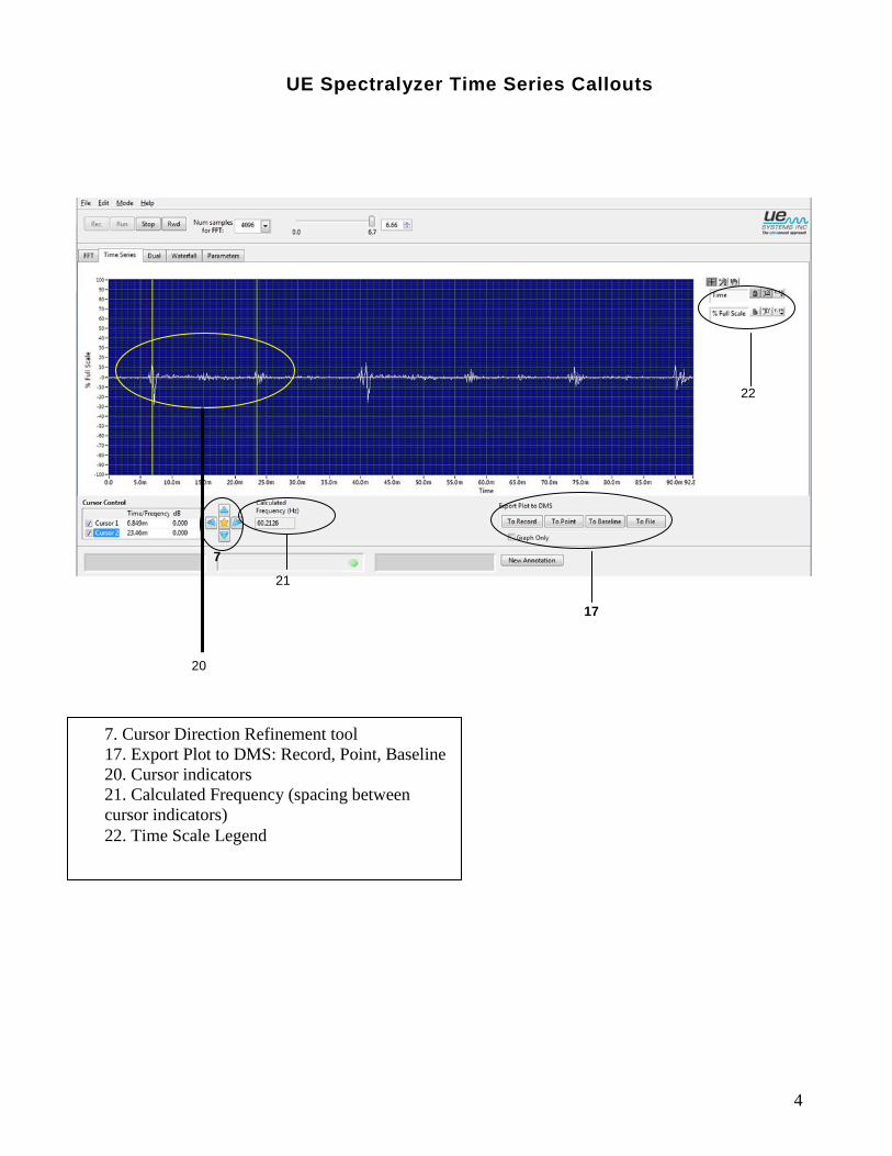
UE Spectralyzer Time Series Callouts

21

20

22

7. Cursor Direction Refinement tool

17. Export Plot to DMS: Record, Point, Baseline

20. Cursor indicators

21. Calculated Frequency (spacing between

cursor indicators)

22. Time Scale Legend

17

7

5

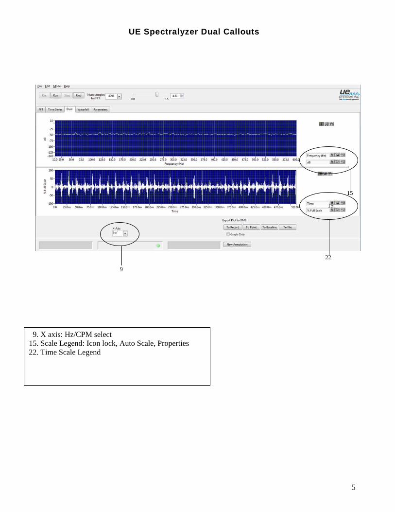
9. X axis: Hz/CPM select

15. Scale Legend: Icon lock, Auto Scale, Properties

22. Time Scale Legend

9

15

UE Spectralyzer Dual Callouts

22

15

6

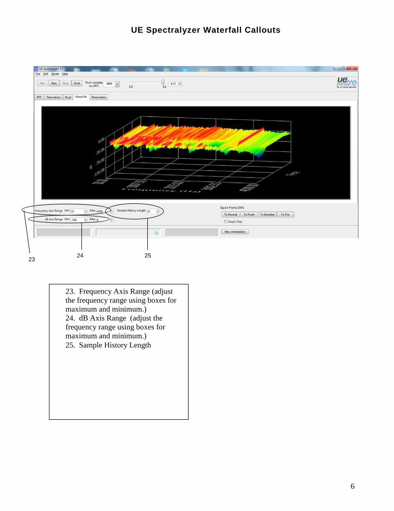
UE Spectralyzer Waterfall Callouts

23 24 25

23. Frequency Axis Range (adjust

the frequency range using boxes for

maximum and minimum.)

24. dB Axis Range (adjust the

frequency range using boxes for

maximum and minimum.)

25. Sample History Length

7

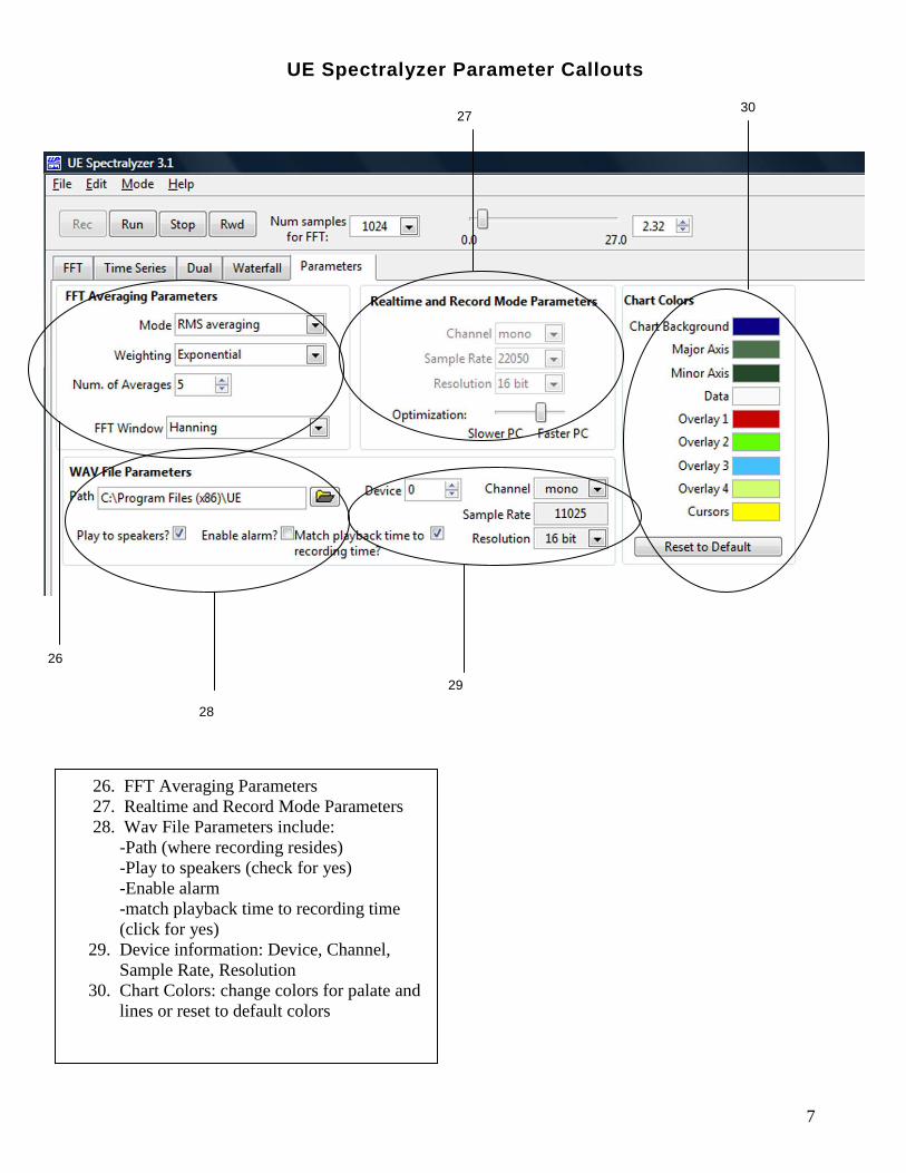
UE Spectralyzer Parameter Callouts

26

27 22

28

29

30

26. FFT Averaging Parameters

27. Realtime and Record Mode Parameters

28. Wav File Parameters include:

-Path (where recording resides)

-Play to speakers (check for yes)

-Enable alarm

-match playback time to recording time

(click for yes)

29. Device information: Device, Channel,

Sample Rate, Resolution

30. Chart Colors: change colors for palate and

lines or reset to default colors

8

Introduction

A spectrum analyzer creates a visual image of sound. It displays the amplitude and frequency components of a recorded sound in a screen that looks similar to that of an oscilloscope (an oscilloscope shows time and amplitude). The frequency limit is set by the parameters of the computer sound card. This is related to the sampling rate capabilities of the sound card. The sampling rate establishes how many times a second the analog input signal is sampled by the sound card.

Authorization

In order to operate your UE Spectralyzer program legally after the free time period, you must register with UE Systems Inc. to receive an authorization code and then enter your authorization code in the UE Spectralyzer program.

Refer to “Registration and Authorization” on following page.

Program Overview

The UE Spectralyzer program provides the user with the tools for performing basic spectral analysis on audible sound images. The program displays spectral (FFT), time series, dual (FFT and time series), waterfall and parametric information on 5 main display windows. The user can open only one of the 5 main display windows at a time by clicking on the corresponding TAB on the program’s main screen. The 5 main display windows are:

FFT Display Window: To view click on the FFT TAB.

Time Series Display Window: To view click on the Time Series TAB.

Dual: To view click the Dual TAB.

Waterfall: To view click on the Waterfall TAB. Parameters Display Window: To view click on the Parameters TAB.

The user can perform program functions by selecting options from the programs main tool bar. The user can control particular aspects of the display windows using program controls. The program controls appear on the scale legend, cursor controls, graph pallet, overlay pallet, and plot legend. Additionally the user can control the operation of the spectral analysis by using the control buttons (REC, RUN, STOP & RWD).

9

System requirements

Operating System requirements

Vista, Windows XP

Installation

If you download from the Internet, locate the file: “Spectralyzer.zip”.

For installation of UE Spectralyzer from your computer, locate the file “Spectralyzer.zip” and extract the contents of the “Spectralyzer.zip”. To install the program double click on “setup.exe” and follow the instructions.

To install UE Spectralyzer from a CD: insert the CD, select My Computer, select the appropriate disc drive and click on the UE Spectralyzer folder, click on the setup.exe” icon and follow the instructions.

Or open the “Start”, “Run” command “setup.exe” and follow the instructions.

Registration and Authorization

In order to operate your UE Spectralyzer program legally after the free trial period, you must register with UE Systems, Inc. and receive an authorization code.

You can use the UE Spectralyzer program for 60 days whether or not you enter an authorization code. After 60 days you will receive a reminder to enter your authorization code. This reminder will continue to pop up until you enter your authorization code.

1. Go to the Help menu and select “Registration Info” Fill out the form and follow the instructions.

2. UE Systems will issue an authorization code. 3. After you receive your authorization code from UES: 4. Open the Help menu and select “Authorization” 5. Enter your authorization number.

10

Main Tool Bar Operations

New Recording

Recording WAV files is quite simple. Just as recording from a tape recorder, make sure that the computer is connected to the sound source (your Ultraprobe) via a cable with a “miniphone” to “miniphone” plug. You may also record from a tape recorder or Minidisk. Adjust the sensitivity volume of the inputting device so as to not overload the recording.

In order to record, the input device must be on. When ready, press the Record button. When finished, press Stop. To save your recording, select the File menu and Save As. If you are not satisfied with your recording or wish to re-record, you may either Rewind and Record or go to the File menu and then select New Recording.

The maximum recording time is 5 minutes, however most sound files should be limited to 10- 30 seconds or less. NOTE: long recordings use a lot of memory. Therefore, you will have to change the sample rate and the optimization bar to accommodate this large cache of memory while recording.

The following are suggested parameters for a typical 30-second recording:

Num samples for FFT: 4096, Sample Rate: 11025. Resolution: 16 bits.

Here are suggested parameters for long files such as a 5-minute recording sample:

Num samples for FFT: 1024, Sample Rate: 8000, Resolution: 8 bits. Slide the Optimization bar to the left.

To change the Sample rate, Click on the arrow indicator of the “Num samples for FFT” box located on the top tool bar.

In the Parameters tab, the sample record rate can be changed only in the Record Mode.

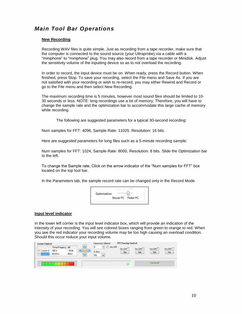
Input level indicator

In the lower left corner is the input level indicator box, which will provide an indication of the intensity of your recording. You will see colored boxes ranging from green to orange to red. When you see the red indicator your recording volume may be too high causing an overload condition. Should this occur reduce your input volume.

11

Opening a WAVE file

To open a recorded WAVE file go to the “File” menu and select “Open WAV file”.

Saving Wave Files

A wave file can be saved after recording or playing a sound sample. In the UE Spectralyzer software you have the option of saving WAV files. Saving is very easy. Go to the “File” menu select “Save as”. Give the file name, choose the location and in which to save this file, and save.

Saving configurations

After creating a configuration, to save a configuration, go to the “File” menu and select “Save Configuration”. Give the configuration a name; check "Save in” to be sure you are saving in the correct location.

Loading Configurations To load a configuration, go to the “File” menu and select “Load Configuration”. Choose configuration and click “open”. Saving Overlays If you wish to save overlays for a specific spectral view, go to the “File” menu, select “Save Overlays” and then select the overlay number you wish to save.

Loading Overlays

To load and overlay, go to the “File” menu and select “Load Overlays”. Then browse to choose the overlay you wish to use. Select it and click “OK”

Reporting

Reporting and printing can be accomplished with UE Spectralyzer software. To create a report, select the “File” menu and then “Reports”. When opened, you'll note that the screen displays the selected WAV file spectrum. Scroll down and you'll find a report box in which you can enter details of your report. When through, select the “File” menu in the report box. You will have a choice of printing a report to window or saving the report has an HTML file.

Edit

Editing is performed in the time series and may be executed in the playback mode or the record mode. With this feature you can shorten WAV files to keep only the area of interest.

To edit, use the zoom tool to highlight the area of interest, then , select the Edit menu. Choose either “Keep only displayed segment” or Delete displayed segment”.

12

Modes

Real-time: In the real-time mode you can use the Spectralyzer as an oscilloscope in that the spectrum will be viewed as it plays a sound. You will not be able to record in real-time. You can only view as it plays.

Record mode: In the record mode you will be able to record your sounds. Make sure that the sound source (your Ultraprobe) is plugged into the mic jack of your computer. In this mode you can record and save your recordings. You cannot open a previously saved recording. You can save the recording when through or re-record without saving.

Playback Mode: In Playback Mode you can open previously recorded wave files and analyze them. You can select overlays and compare up to four wave files. Previously saved configurations can be opened for analysis.

Control Buttons

Recording & Saving WAVE Files

Recording WAVE files is quite simple. Just as recording from a tape recorder, make sure that the computer is connected to the sound source (your Ultraprobe) via a cable with “miniphone” plug on the end that plugs into the computer. You may also record from a tape recorder or MP3 recorder. Adjust the volume of the inputting device (example your Ultraprobe) so as to not overload the recording. Look at the input level indicator to see if the input is overloading.

In order to record, the input device must be on. When ready, press the “Record” icon. When finished, select “Stop”. To save your recording, select the “File” menu and “Save As”. If you are not satisfied with your recording or wish to re-record, you may either rewind and record or go to the “File” menu and then select “New Recording”.

To do this, click “Stop” and then click on “Rewind”, open the “File” menu and select “New Recording”.

13

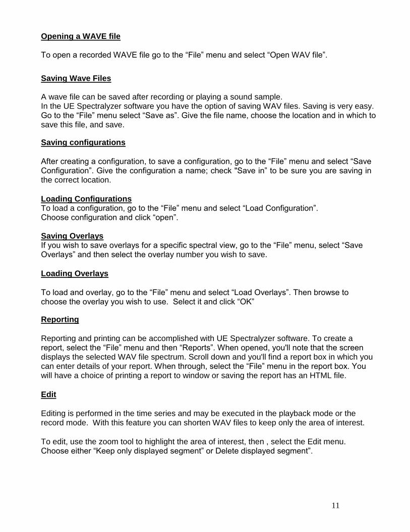
Playing a WAVE File

To play a WAVE file, go to File menu, select “Open WAV file”. Then, “Run”. When finished playing, click “Stop”. To hear any segment of a recorded WAV file you may either choose rewind or move the time slider bar of the seconds counter right or left. This bar is located in the top right side of the spectra

display.

Program Controls

Scale Legend

Properties of the Frequency and dB axis can be adjusted with the Scales Legend control located below the plot to the left.

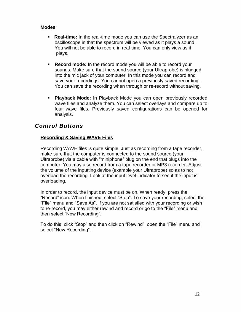
Frequency Axis

1. Axis Name 2. Lock Icon: 3. Auto Scale Icon: 4. Properties Icon:

1 2 3 4

DB Axis

1. Axis Name 2. Lock Icon: 3. Auto Scale Icon 4. Properties Icon:

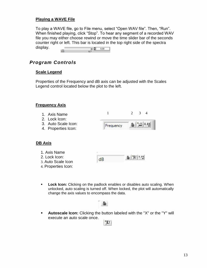
Lock Icon: Clicking on the padlock enables or disables auto scaling. When unlocked, auto scaling is turned off. When locked, the plot will automatically change the axis values to encompass the data.

Autoscale Icon: Clicking the button labeled with the "X" or the "Y" will execute an auto scale once.

14

Should you be out of range and are not able to view the spectrum, go to the frequency or the dB boxes located on the bottom of your screen. The auto scale icons are located next to the lock icon. To center or optimize the Spectrum, simply click on either the frequency or the decibel auto scale icons.

Properties Icon: Clicking on the "X.XX" or "Y.YY" buttons opens a menu that allows the user to modify axis attributes such as linear/log, precision, color, etc.

Cursors

There are two cursors that can be viewed in the FFT and in the time series screens to help determine frequency and dB levels. Each cursor has a horizontal and a vertical bar. The vertical bar will display the frequency in the cursor box and the horizontal line will display the decibel level in the cursor box. The cursor box is shown in the lower middle of the screen.

Calculated Frequencies

In the time series two vertical markers are used to mark the peaks of interest. The calculated frequency between them will be indicated in the Calculated Frequency Box.

Cursor Legend

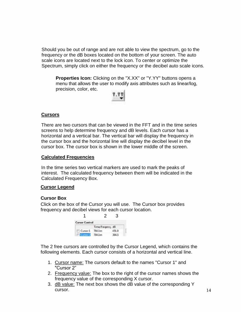
Cursor Box

Click on the box of the Cursor you will use. The Cursor box provides frequency and decibel views for each cursor location.

1 2 3

The 2 free cursors are controlled by the Cursor Legend, which contains the following elements. Each cursor consists of a horizontal and vertical line.

1. Cursor name: The cursors default to the names "Cursor 1" and "Cursor 2”

2. Frequency value: The box to the right of the cursor names shows the frequency value of the corresponding X cursor.

3. dB value: The next box shows the dB value of the corresponding Y cursor.

15

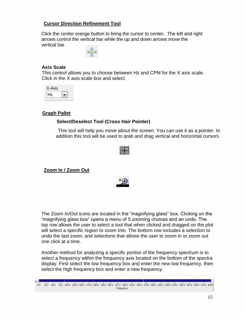
Cursor Direction Refinement Tool

Click the center orange button to bring the cursor to center. The left and right arrows control the vertical bar while the up and down arrows move the vertical bar.

Graph Pallet

Select/Deselect Tool (Cross Hair Pointer)

This tool will help you move about the screen. You can use it as a pointer. In addition this tool will be used to grab and drag vertical and horizontal cursors.

Zoom In / Zoom Out

The Zoom In/Out icons are located in the “magnifying glass” box. Clicking on the “magnifying glass box” opens a menu of 5 zooming choices and an undo. The top row allows the user to select a tool that when clicked and dragged on the plot will select a specific region to zoom into. The bottom row includes a selection to undo the last zoom, and selections that allows the user to zoom in or zoom out one click at a time. Another method for analyzing a specific portion of the frequency spectrum is to select a frequency within the frequency axis located on the bottom of the spectra display. First select the low frequency box and enter the new low frequency, then select the high frequency box and enter a new frequency.

Axis Scale This control allows you to choose between Hz and CPM for the X axis scale. Click in the X axis scale box and select.

16

Overlay pallet & Overlays

There are four Overlays from which to choose. You can adjust the color in the parameters tab (see Changing Palate and Line colors)

You may adjust the view of an overlay by clicking on the desired number of the overlay you wish to view and then select line style, line width, or a specific plot view such as: Bar Plots, Fill Base Line, Interpolation or Point Style.

To select an overlay, click the “On-Off” button and to set the overlay, click the “Set” button.

One may save an overlay by selecting “File” and then "save overlay" . To load an overlay that has been previously saved, go to “File” and then select “Load overlays”. Alarm Set In the FFT view alarms can be set.

To set an alarm: 1. Choose the “Select/Deselect”, (Cross Hair Pointer) tool. 2. Turn Cursor 1 on. 3. Open the cursor format button and scroll down to "Bring to Center". 4. Using the Cross Hair Cursor, drag the vertical cursor to the first, low

frequency set point. 5. Use the Cross Hair Cursor to drag the horizontal cursor to the desired

decibel threshold limit. 6. Turn Cursor 2 on.

7. Open the Cursor 2 format button and scroll down to “Bring to Center”. 8. Using the Cross Hair Cursor, drag the Cursor 2 vertical line to where

you want the desired upper frequency setpoint to be.

When the decibel threshold within the selected frequency spectrum is exceeded, the alarm box button will turn from green to red. The date and time of the alarm will be displayed.

8. 9.

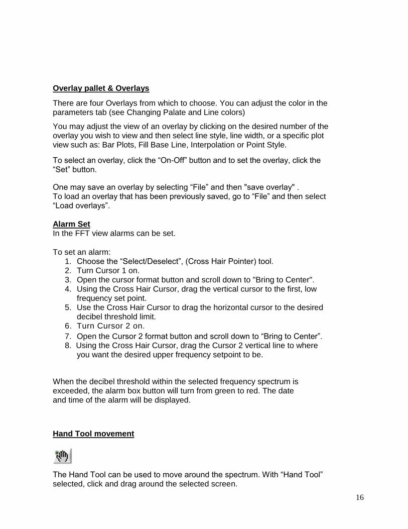
Hand Tool movement

The Hand Tool can be used to move around the spectrum. With “Hand Tool” selected, click and drag around the selected screen.

17

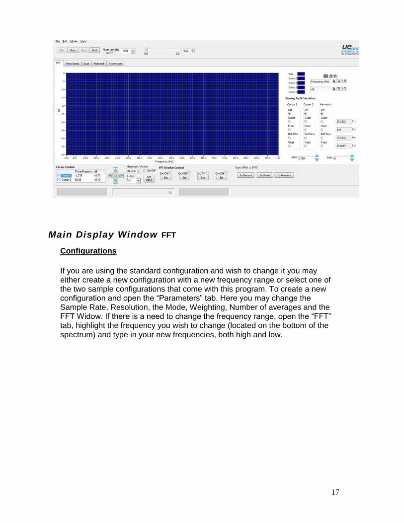
Main Display Window FFT

Configurations

If you are using the standard configuration and wish to change it you may either create a new configuration with a new frequency range or select one of the two sample configurations that come with this program. To create a new configuration and open the “Parameters” tab. Here you may change the Sample Rate, Resolution, the Mode, Weighting, Number of averages and the FFT Widow. If there is a need to change the frequency range, open the “FFT” tab, highlight the frequency you wish to change (located on the bottom of the spectrum) and type in your new frequencies, both high and low.

18

Adjusting DB scale

The method to adjust the dB scale is similar to that of adjusting the frequency range. Highlight the low end or the high end of the decibel range and type in your new parameters. As with frequency adjust you can also use the magnifier icon and move to the spectrum decibel range you wish to view. Time Series

You may view an event in Time Series. Here a selected sound sample may be viewed as changes in amplitude over time.

Time adjustment

As with frequency adjustment, the time view may be changed. To do this, select the magnifier tool located in the magnifier toolbox.

Waterfall

This is a 3-D view of frequency, and decibel over time as it plays. Adjustments include: frequency axis range (min & max), dB axis range (min & max) and sample history length.

Parameters

You may customize the appearance of the spectrum view (FFT) and Time series by using or changing information in the parameters tab.

FFT Averaging Parameters

1. Mode: View selections as peak hold, no averaging, vector averaging, RMS averaging. The program initially is set to RMS averaging.

2. Weighting: There are two selections for weighting: exponential and linear. Exponential weighting is used most often.

3. FFT Window: Here is where you'll select the view of your spectrum. You can select different sampling windows such as: None, Hanning, Hamming, Blackman -- Harris, Exact Blackman, Blackman, Flat Top, 4 term B -- Harris, Low Sidelobe. The software defaults to the Hanning window view.

Real-time and Record Mode Parameters

You may adjust the recording parameters here. The parameters may only be changed while you are in the recording mode. There are four selections for recording:

1. Channel: The default is mono.

19

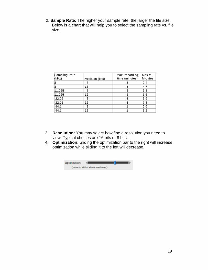
2. Sample Rate: The higher your sample rate, the larger the file size.

Below is a chart that will help you to select the sampling rate vs. file size.

Sampling Rate (kHz) Precision (bits)

Max Recording time (minutes)

Max # M-bytes

8 8 5 2.4

8 16 5 4.7

11.025 8 5 3.3

11,025 16 5 6.5

22.05 8 3 3.9

22.05 16 3 7.8

44.1 8 1 2.6

44.1 16 1 5.2

3. Resolution: You may select how fine a resolution you need to view. Typical choices are 16 bits or 8 bits.

4. Optimization: Sliding the optimization bar to the right will increase optimization while sliding it to the left will decrease.

20

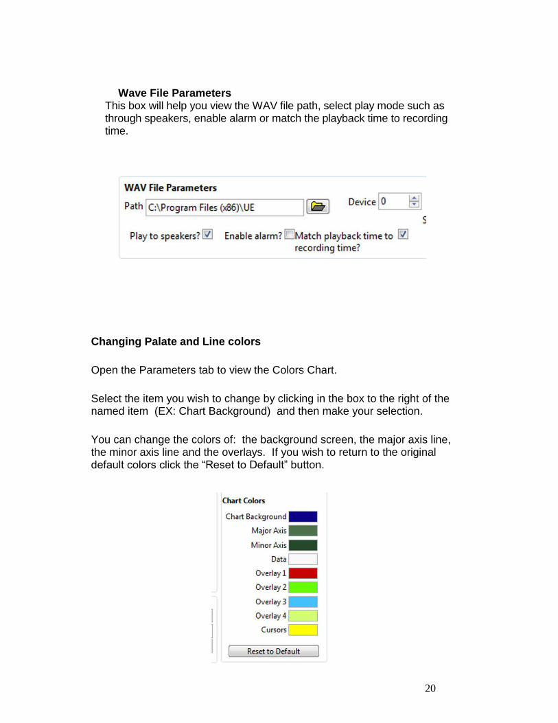
Wave File Parameters This box will help you view the WAV file path, select play mode such as through speakers, enable alarm or match the playback time to recording time.

Changing Palate and Line colors

Open the Parameters tab to view the Colors Chart.

Select the item you wish to change by clicking in the box to the right of the named item (EX: Chart Background) and then make your selection.

You can change the colors of: the background screen, the major axis line, the minor axis line and the overlays. If you wish to return to the original default colors click the “Reset to Default” button.

21

Additional Features

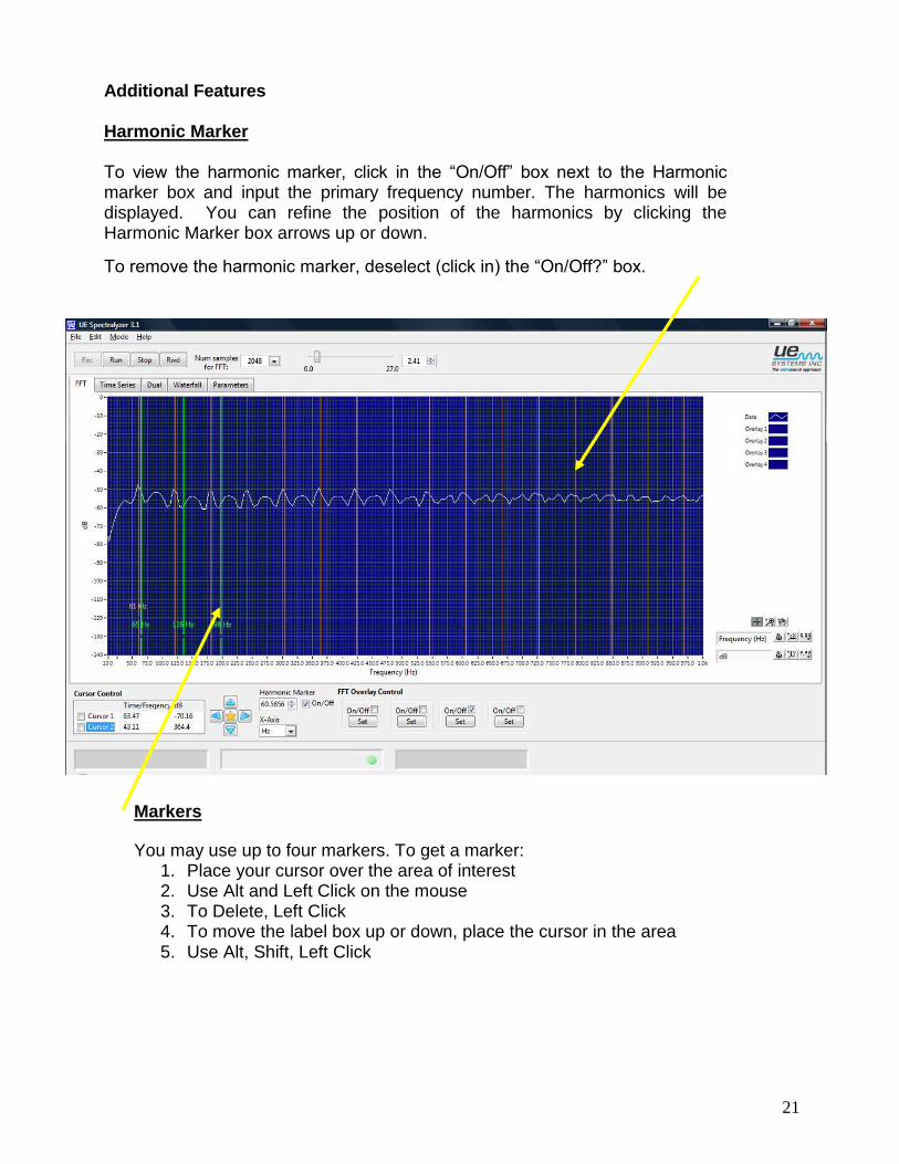
Harmonic Marker

To view the harmonic marker, click in the “On/Off” box next to the Harmonic marker box and input the primary frequency number. The harmonics will be displayed. You can refine the position of the harmonics by clicking the Harmonic Marker box arrows up or down.

To remove the harmonic marker, deselect (click in) the “On/Off?” box.

Markers

You may use up to four markers. To get a marker: 1. Place your cursor over the area of interest 2. Use Alt and Left Click on the mouse 3. To Delete, Left Click 4. To move the label box up or down, place the cursor in the area 5. Use Alt, Shift, Left Click

22

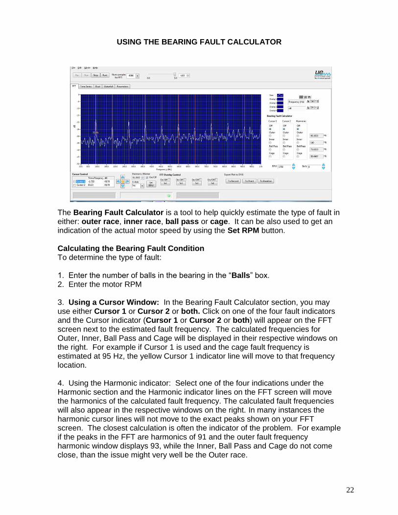
USING THE BEARING FAULT CALCULATOR

The Bearing Fault Calculator is a tool to help quickly estimate the type of fault in either: outer race, inner race, ball pass or cage. It can be also used to get an indication of the actual motor speed by using the Set RPM button.

Calculating the Bearing Fault Condition To determine the type of fault: 1. Enter the number of balls in the bearing in the “Balls” box. 2. Enter the motor RPM 3. Using a Cursor Window: In the Bearing Fault Calculator section, you may use either Cursor 1 or Cursor 2 or both. Click on one of the four fault indicators and the Cursor indicator (Cursor 1 or Cursor 2 or both) will appear on the FFT screen next to the estimated fault frequency. The calculated frequencies for Outer, Inner, Ball Pass and Cage will be displayed in their respective windows on the right. For example if Cursor 1 is used and the cage fault frequency is estimated at 95 Hz, the yellow Cursor 1 indicator line will move to that frequency location. 4. Using the Harmonic indicator: Select one of the four indications under the Harmonic section and the Harmonic indicator lines on the FFT screen will move the harmonics of the calculated fault frequency. The calculated fault frequencies will also appear in the respective windows on the right. In many instances the harmonic cursor lines will not move to the exact peaks shown on your FFT screen. The closest calculation is often the indicator of the problem. For example if the peaks in the FFT are harmonics of 91 and the outer fault frequency harmonic window displays 93, while the Inner, Ball Pass and Cage do not come close, than the issue might very well be the Outer race.

23

5. Set RPM: should the harmonic cursor lines in the FFT screen not match exactly with the fault calculations as indicated in the windows on the right of the screen, it might be the motor frequency is not correct. To determine the motor frequency: a.) Be sure the calculated fault in the Harmonic section is selected (Outer, Inner, Ball Pass or Cage). b.) Move harmonic marker by pressing the up/down arrows in the Harmonic Marker window to move the harmonic cursor over the harmonic peak. c.) Once you have the harmonic cursor over the harmonic peak, you then click on “Calculate RPM”. The RPM you now have is close to the actual RPM speed of the motor. The RPM that is calculated is what the RPM would be for the type of fault and the number of balls indicated based on where the marker is placed.

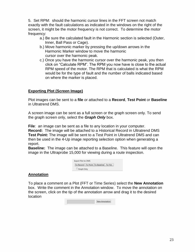
Exporting Plot (Screen Image)

Plot images can be sent to a file or attached to a Record, Test Point or Baseline in Ultratrend DMS. A screen image can be sent as a full screen or the graph screen only. To send the graph screen only, select the Graph Only box. File: an image can be sent as a file to any location in your computer. Record: The image will be attached to a Historical Record in Ultratrend DMS Test Point: The image will be sent to a Test Point in Ultratrend DMS and can then be used in the 4-Up image reporting selection option when generating a report. Baseline: The image can be attached to a Baseline. This feature will open the image in the Ultraprobe 15,000 for viewing during a route inspection. Annotation To place a comment on a Plot (FFT or Time Series) select the New Annotation box. Write the comment in the Annotation window. To move the annotation on the screen, click on the tip of the annotation arrow and drag it to the desired location

24

Appendix A Summary of Controls & Indicators Descriptions Tab Control Choose between the FFT, Time Series, Dual, Waterfall or Parameters displays.

FFT Averaging Parameters averaging parameters is a cluster that defines how the averaging is computed.

Mode Averaging mode specifies the averaging mode used in the FFT calculation

Weighting This Mode specifies the weighting mode used for RMS and Vector averaging.

Number of avgs Number of averages specifies the number of averages that is used for RMS and Vector averaging. If weighting mode is Exponential, the averaging process is continuous. If weighting mode is Linear, the averaging process resets automatically once the selected number of averages have been computed.

Realtime and Record Mode Properties identifies how the sound operation is set up (Mono or Stereo), its sampling rate, and whether it set up as 8- or 16-bit sound. This information is used in Realtime and Record modes.

Channel Always reads Mono (stereo is not supported)

Sample Rate Indicates the sample rate used when acquiring data in Realtime and Record modes.

Resolution Indicates whether sound will be recorded in 8 bit or 16 bit resolution in Realtime and Record modes.

WAV file Path Wave File Path specifies where the WAV file is located. Clicking on the folder icon displays an

"Open File

" dialog box.

Run Button Pressing the Run Button begins the following actions:

1. Realtime mode, this begins the processing of sound data from the input signal. Data is not saved.

2. Record mode, this begins playback of sound saved in the recording buffer. If the Box "Play to speakers?

" Box is checked (Parameters tab), playback will then be routed to

the computer’s speakers.

3. In ”Playback

” mode, this begins playback of sound data from the specified WAV file.

Stop Button Pressing the Stop Button stops the capture of sound in Realtime and Record modes, and stops the playback of prerecorded sound in Record and Playback modes.

The Stop Button will also reset the Time Series plot to show all recorded data in situations where it is only showing a subset of the data.

Rewind Button Pressing the Rewind Button moves the playback position to the beginning of the

25

recording when in Record or Playback modes.

Record Button Pressing the Record Button begins the recording of sound to a buffer when in Record Mode.

Buffer Pos Slider The Buffer Position Slider indicates the length of the recording in seconds, and shows the current location of the playback. The user can move the slider to select a particular point in the recording. This control is not available in Realtime mode, since sound data is not buffered.

When selecting a particular point in the recording, the FFT and Time Series displays will show data from that particular acquisition time.

Num Samples for FFT sets the number of samples used for calculating the FFT spectrum. This value can be changed while sound data is being captured in Realtime mode. Note that operation at small values can cause buffer overflows when the CPU is busy with other tasks. Use the Optimization Slider (Parameters Tab) to improve performance for slower computers.

Hint: when recording, use a value of 4096 or greater for best performance. You can replay the recording at smaller values without any loss of information.

Playback timing If this option is selected, the playback time in Record and Playback modes will match the recording time. (When not selected, the data being plotted to the FFT or Time Series plot can occur at a much faster rate than the recording time.)

Note: When "Play to speakers?

" is checked, it is suggested that this checkbox be checked as

well.

Play to speakers? When this option is chosen, sound will be played to the speakers in either Record mode or Playback mode.

FFT Overlay Control

The 4 "On/Off

" buttons toggle the corresponding Overlay trace on or off. If the Overlay trace

“Set

” Button has not been clicked, clicking the On/Off button has no effect.

Set Overlay

The 4 "Set

" buttons create an overlay of the current FFT trace. The overlay trace can be turned

on or off with the corresponding on/off button.

Optimization Use this slider to optimize the program's performance for your machine if you are

receiving errors when recording data in the "Record

" mode. For slower computers, choose a

value farther to the left; for faster computers, use a value toward the right.

Cursors On/Off

The 2 "Cursor On/Off

" buttons toggles the corresponding free cursor on and off. The cursor

legend (found below the FFT plot) contains additional cursor control functions.

26

FFT Graph The FFT Graph displays an FFT of the captured data, using the number of samples selected in the

"Num Samples for FFT

" control. The Averaging and Window parameters on the

Parameters tab are inputs into the FFT algorithm. The update rate is limited by either the speed of the computer or by the time required to acquire the data sent to the FFT algorithm. The FFT plot also can show overlay data if selected.

Notes on FFT span, bins and resolution:

1. The number of FFT bins is always 1/2 of the number of samples used to calculate the FFT. For example, 4096 samples will equal an FFT with 2048 bins.

2. The FFT span is 1/2 of the sampling rate selected in the parameters tab. At a sampling rate of 22050 samples per second, you will have an FFT span of 11025 Hz. No data is plotted at frequency values higher than the FFT span or at values less than 0.

3. The FFT resolution is the FFT span / # FFT bins. The user can control

several types of cursors with on the FFT plot:

1. Free cursors: There are 2 free cursors for identifying horizontal and vertical coordinates. The cursor palette just below the graph controls these cursors. They can be turned on and off with the on/off buttons at the lower left of the FFT tab.

2. Markers: Four markers are available for tagging specific points on the FFT display. To place a marker, use

"Alt-left click

". To remove a marker, simply click on it with a left mouse click. To

shift the text to a new position (vertically), use "Shift-Alt-left click

". The horizontal position of the

markers is fixed.

3. Harmonic Cursors: To display harmonic cursors, use "Shift-left click

". Cursors are placed at

multiple integers of the frequency value selected by the click. This value is displayed for reference. To shift the text to a new position (vertically), use

"Shift-Alt-left click

". To remove

the harmonic cursors, use "Control-left click

"

The FFT plot contains 4 controls:

1. Scale Legend: Properties of the Frequency and dB axis can be adjusted with the Scales Legend control located below the plot to the left. It contains the following elements:

a. Axis name: These are set to "Frequency

" and

"dB

".

b. Autoscale lock: Clicking on the padlock enables or disables autoscaling. When unlocked, autoscaling is turned off. When locked, the plot will automatically change the axis values to encompass the data.

c. Single-shot autoscale: Clicking the button labeled with the "X" or the "Y" will execute an autoscale once.

d. Axis format: Clicking on the "X.XX

" or

"Y.YY

" buttons opens a menu that allows the

user to modify axis attributes such as linear/log, precision, color, etc.

2. Cursor Legend: The 2 free cursors are controlled by the Cursor Legend, which contains the following elements. Each cursor consists of a horizontal and vertical line.

27

a. Cursor name: The cursors default to the names "Cursor 1" and

"Cursor 2"

b. Frequency value: The box to the right of the cursor names shows the frequency value of the corresponding X cursor.

c. dB value: The next box shows the dB value of the corresponding Y cursor.

d. Select tool: The clicking on one of the crosshair buttons selects the corresponding cursor (see nudge tool below).

e. Cursor format: The next button opens a menu that allows the user to modify cursor attributes such as style, width, color, etc.

f. Cursor lock: Clicking on the padlock allows the user to select whether the Y cursor will float freely or lock to a plot.

3. Nudge tool: Clicking on one of the directional diamonds will nudge the selected cursor (see select tool above) 1 pixel in the selected direction.

4. Graph Palette: The Graph Palette allows the user to zoom and pan the plot. It consists of the following elements:

a. Deselect tool: Clicking on the crosshairs deselects any of the zoom or pan tools that were selected.

b. Zoom tools: Clicking on the magnifying glass opens a menu of 5 zooming choices and an undo. The top row allows the user to select a tool that when clicked and dragged on the plot will select a specific region to zoom into. The bottom row includes a selection to undo the last zoom, and selections that allow the user to zoom in or zoom out one click at a time.

c. Pan tool: Clicking the hand icon selects a panning tool that allows the user to click and drag on the plot in a panning mode.

5. Plot Legend: The Plot Legend displays a colored line when the corresponding overlay trace is enabled. Clicking on the line will bring up a menu that allows the user to set trace attributes such as line width, color, line type, etc.

Time Series Graph Displays the Amplitude vs. Time display of either captured or prerecorded sound data. Vertical scaling is in % of full scale.

While running, this graph shows the amplitude information of the most recently acquired "chunk

" of

data. This is also the case when displaying the data obtained after the playback position has been manually changed via the Buffer Position Slider. In these cases, the Time axis shows with respect to the current

"chunk

" as opposed to the time within the recording. The

"chunk

" time can easily be calculated

from the current sampling rate and the number of samples used for the FFT. i.e.: At 22050 Samples/sec, with 16384 Num samples, the chunk time is 16384/22050 = ~743ms.

Horizontal and vertical scale properties can be adjusted with the Scales palette located just below and to the left of the graph. The Graph palette below and to the right can be used for zooming as described in the help for the FFT plot. Note that the % Full Scale can be greater than 100% to show the full wave form

In Record and Playback modes, the segment viewed can be either deleted from recording or kept via the appropriate menu options in the Edit menu.

Need Help? Want information regarding products or training?

Contact UE Systems, Inc.

Email: info@uesystems.com Internet: http://www.uesystems.com

Phone: +914-592-1220 Fax: +914-347-2181