U n i v e r s i t y o f S o u t h e r n Q u e e n s l a n d Neural Networks and Self-Organising...

U n i v e r s i t y o f S o u t h e r n Q u e e n s l a n d

www.usq.edu.au

Neural Networks and Neural Networks and Self-Organising MapsSelf-Organising Maps

CSC3417CSC3417Semester 1, 2007Semester 1, 2007

T h e U n i v e r s i t y o f S o u t h e r n Q u e e n s l a n dU n i v e r s i t y o f S o u t h e r n Q u e e n s l a n d

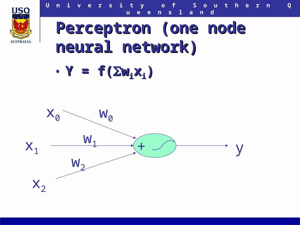
Perceptron (one node neural Perceptron (one node neural network)network)

• Y = f(Y = f(wwiixxii))

+

w0

w1

w2

x0

x1

x2

y


R Code for a PerceptronR Code for a Perceptron

• step <- function(sigma) {step <- function(sigma) {• if (sigma<0) { if (sigma<0) { • return (0);return (0);• } else { return (1); }} else { return (1); }• }}

• neural <- function(weights,inputs,output,eta) {neural <- function(weights,inputs,output,eta) {• sigma <- t(inputs) %*% weights;sigma <- t(inputs) %*% weights;• yhat <- step(sigma);yhat <- step(sigma);• diff <- output-yhat;diff <- output-yhat;• for (k in 1:length(weights)) {for (k in 1:length(weights)) {• weights[[k]] <- weights[[k]] + eta*inputs[[k]]*diff;weights[[k]] <- weights[[k]] + eta*inputs[[k]]*diff;• }}• return (weights);return (weights);• }}

Start with randomweights and use thisfunction iteratively.


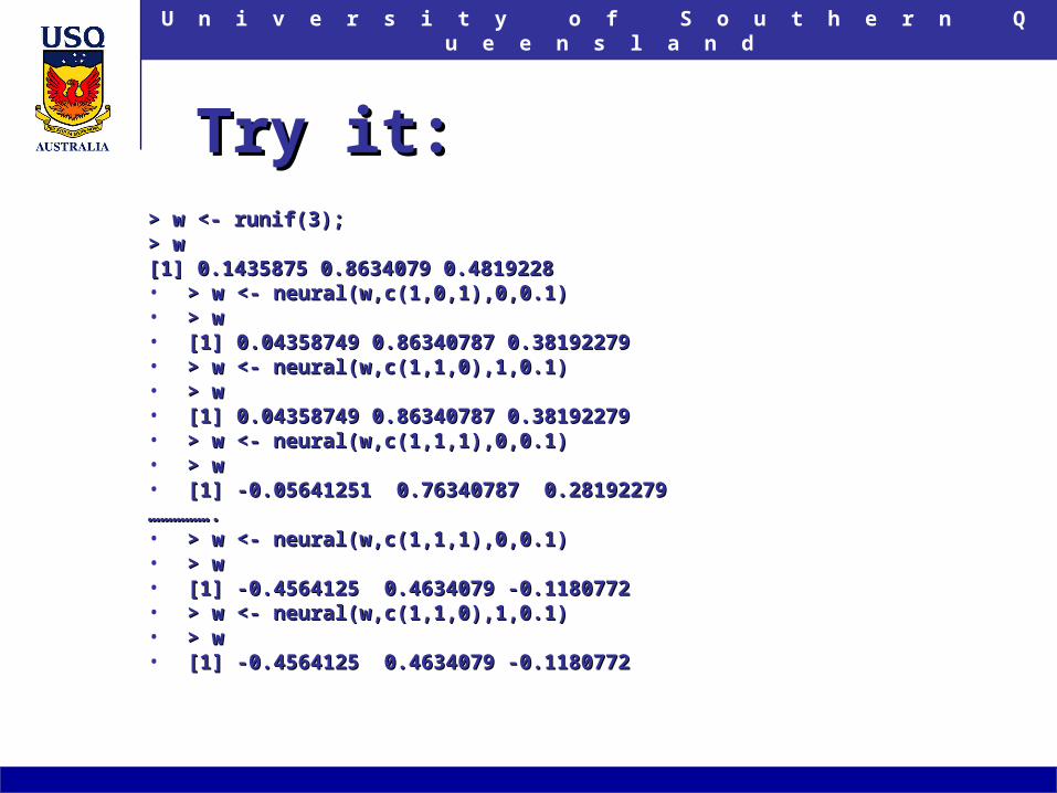
Try it:Try it:> w <- runif(3);> w <- runif(3);> w> w[1] 0.1435875 0.8634079 0.4819228[1] 0.1435875 0.8634079 0.4819228• > w <- neural(w,c(1,0,1),0,0.1)> w <- neural(w,c(1,0,1),0,0.1)• > w> w• [1] 0.04358749 0.86340787 0.38192279[1] 0.04358749 0.86340787 0.38192279• > w <- neural(w,c(1,1,0),1,0.1)> w <- neural(w,c(1,1,0),1,0.1)• > w> w• [1] 0.04358749 0.86340787 0.38192279[1] 0.04358749 0.86340787 0.38192279• > w <- neural(w,c(1,1,1),0,0.1)> w <- neural(w,c(1,1,1),0,0.1)• > w> w• [1] -0.05641251 0.76340787 0.28192279[1] -0.05641251 0.76340787 0.28192279…………………………..• > w <- neural(w,c(1,1,1),0,0.1)> w <- neural(w,c(1,1,1),0,0.1)• > w> w• [1] -0.4564125 0.4634079 -0.1180772[1] -0.4564125 0.4634079 -0.1180772• > w <- neural(w,c(1,1,0),1,0.1)> w <- neural(w,c(1,1,0),1,0.1)• > w> w• [1] -0.4564125 0.4634079 -0.1180772[1] -0.4564125 0.4634079 -0.1180772


Scilab versionScilab version

function [stp] = step (sigma)function [stp] = step (sigma) if sigma<0if sigma<0 stp = 0;stp = 0; else else stp = 1; stp = 1; endendendfunctionendfunction

function [w] = neural(weights,inputs,output,eta) function [w] = neural(weights,inputs,output,eta) sigma = weights * inputs';sigma = weights * inputs'; yhat = step(sigma);yhat = step(sigma); diff = output-yhat;diff = output-yhat; w = weights;w = weights; for k=1:length(weights) for k=1:length(weights) w(k) = weights(k) + eta*inputs(k)*diff;w(k) = weights(k) + eta*inputs(k)*diff; endendendfunctionendfunction


Try it:Try it:

-->w = rand(1,3)-->w = rand(1,3) w =w = 0.6653811 0.6283918 0.84974520.6653811 0.6283918 0.8497452

-->w = neural(w,[1,0,1],0,0.1)-->w = neural(w,[1,0,1],0,0.1) w =w = 0.5653811 0.6283918 0.74974520.5653811 0.6283918 0.7497452

-->w = neural(w,[1,1,0],1,0.1)-->w = neural(w,[1,1,0],1,0.1) w =w = 0.5653811 0.6283918 0.74974520.5653811 0.6283918 0.7497452

-->w = neural(w,[1,1,1],0,0.1)-->w = neural(w,[1,1,1],0,0.1) w =w = 0.4653811 0.5283918 0.64974520.4653811 0.5283918 0.6497452………………....


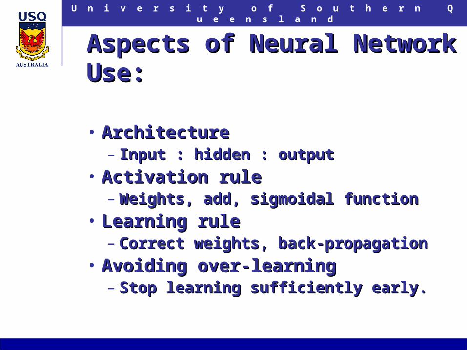
Aspects of Neural Network Use:Aspects of Neural Network Use:

• ArchitectureArchitecture– Input : hidden : outputInput : hidden : output

• Activation ruleActivation rule– Weights, add, sigmoidal functionWeights, add, sigmoidal function

• Learning ruleLearning rule– Correct weights, back-propagationCorrect weights, back-propagation

• Avoiding over-learningAvoiding over-learning– Stop learning sufficiently early.Stop learning sufficiently early.


Multilayer networksMultilayer networks

• Learning by back-propagation.Learning by back-propagation.


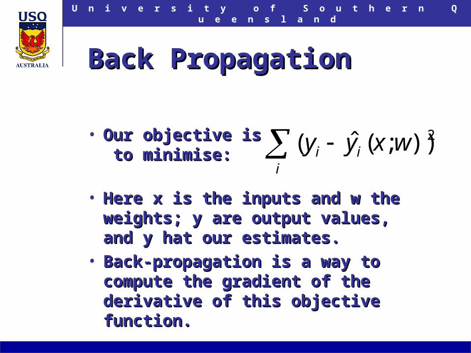
Back PropagationBack Propagation

• Our objective isOur objective is to minimise: to minimise:

• Here x is the inputs and w the Here x is the inputs and w the weights; y are output values, and y weights; y are output values, and y hat our estimates.hat our estimates.

• Back-propagation is a way to Back-propagation is a way to compute the gradient of the compute the gradient of the derivative of this objective function.derivative of this objective function.

2));(ˆ( wxyyi

ii


How to avoid overfittingHow to avoid overfitting

• Stop learning earlyStop learning early• Reduce the learning speedReduce the learning speed• Bayesian approach:Bayesian approach:– ““The The overfitting problemoverfitting problem can be can be

solve by using a Bayesian solve by using a Bayesian approach to control model approach to control model complexity.” MacKay, Information complexity.” MacKay, Information theory, Inference and Learning theory, Inference and Learning Algorithms, CUP, 2003.Algorithms, CUP, 2003.


Advantages of Bayesian Advantages of Bayesian Approach (MacKay 2003)Approach (MacKay 2003)

1.1. No ‘test set’ required No ‘test set’ required – hence more data efficient.– hence more data efficient.

2.2. Overfitting parameters just appear Overfitting parameters just appear as ordinary parameters.as ordinary parameters.

3.3. Bayesian objective function is Bayesian objective function is smooth, hence easier to optimize.smooth, hence easier to optimize.

4.4. Gradient of objective function can Gradient of objective function can be evaluated.be evaluated.

McKay’s book is online:http://www.inference.phy.cam.

ac.uk/mackay/Book.html


Self-organising MapsSelf-organising Maps• Each node has a vector Each node has a vector

of parameters of the of parameters of the same dimension as the same dimension as the inputs.inputs.

• Training moves nodes Training moves nodes in the neighbourhood in the neighbourhood of the closest node to of the closest node to an input closer to each an input closer to each other.other.

• Many choices of Many choices of neighbourhood and neighbourhood and adjustment are adjustment are possible.possible.


Neighbourhood and adjustmentNeighbourhood and adjustment

),()(1 tici

ti

ti mxdthmm

wherewhere

andand

.,0

),()(

otherwise

Nttth c

ci

)(exp)(

2

t

rrt ic

U n i v e r s i t y o f S o u t h e r n Q u e e n s l a n d Neural Networks and Self-Organising...

Documents

Transcript of U n i v e r s i t y o f S o u t h e r n Q u e e n s l a n d Neural Networks and Self-Organising...