U N I V E R S I T Y O F C O P E N H A G E NU N I V E R S I...
138
UNIVERSITY OF COPENHAGEN UNIVERSITY OF COPENHAGEN Welcome to Copenhagen! Schedule: Monday Tuesday Wednesday Thursday Friday 8 Registration and welcome 9 Crash course on Differential and Riemannian Geometry 1.1 (Feragen) Crash course on Differential and Riemannian Geometry 3 (Lauze) Introduction to Information Geometry 3.1 (Amari) Information Geometry & Stochastic Optimization 1.1 (Hansen) Information Geometry & Stochastic Optimization in Discrete Domains 1.1 (Màlago) 10 Crash course on Differential and Riemannian Geometry 1.2 (Feragen) Tutorial on numerics for Riemannian geometry 1.1 (Sommer) Introduction to Information Geometry 3.2 (Amari) Information Geometry & Stochastic Optimization 1.2 (Hansen) Information Geometry & Stochastic Optimization in Discrete Domains 1.2 (Màlago) 11 Crash course on Differential and Riemannian Geometry 1.3 (Feragen) Tutorial on numerics for Riemannian geometry 1.2 (Sommer) Introduction to Information Geometry 3.3 (Amari) Information Geometry & Stochastic Optimization 1.3 (Hansen) Information Geometry & Stochastic Optimization in Discrete Domains 1.3 (Màlago) 12 Lunch Lunch Lunch Lunch Lunch 13 Crash course on Differential and Riemannian Geometry 2.1 (Lauze) Introduction to Information Geometry 2.1 (Amari) Information Geometry & Reinforcement Learning 1.1 (Peters) Information Geometry & Stochastic Optimization 1.4 (Hansen) Information Geometry & Cognitive Systems 1.1 (Ay) 14 Crash course on Differential and Riemannian Geometry 2.2 (Lauze) Introduction to Information Geometry 2.2 (Amari) Information Geometry & Reinforcement Learning 1.2 (Peters) Information Geometry & Stochastic Optimization 1.5 (Hansen) Information Geometry & Cognitive Systems 1.2 (Ay) 15 Introduction to Information Geometry 1.1 (Amari) Introduction to Information Geometry 2.3 (Amari) Information Geometry & Reinforcement Learning 1.3 (Peters) Stochastic Optimization in Practice 1.1 (Hansen) Information Geometry & Cognitive Systems 1.3 (Ay) 16 Introduction to Information Geometry 1.2 (Amari) Introduction to Information Geometry 2.4 (Amari) Social activity/ Networking event Stochastic Optimization in Practice 1.2 (Hansen) Information Geometry & Cognitive Systems 1.3 (Ay) Coffee breaks at 10:00 and 14:45 (no afternoon break on Wednesday) Slide 1/57 — Aasa Feragen and François Lauze — Differential Geometry — September 22
-
Upload
duongkhanh -
Category
Documents
-
view
216 -
download
2
Transcript of U N I V E R S I T Y O F C O P E N H A G E NU N I V E R S I...

U N I V E R S I T Y O F C O P E N H A G E N U N I V E R S I T Y O F C O P E N H A G E N
Welcome to Copenhagen!Schedule:
Monday Tuesday Wednesday Thursday Friday8 Registration and
welcome9
Crash course on Differential and
Riemannian Geometry 1.1
(Feragen)
Crash course on Differential and
Riemannian Geometry 3
(Lauze)
Introduction to Information Geometry
3.1(Amari)
Information Geometry & Stochastic Optimization
1.1(Hansen)
Information Geometry & Stochastic Optimization in Discrete Domains 1.1
(Màlago)
10Crash course on Differential and
Riemannian Geometry 1.2
(Feragen)
Tutorial on numerics for Riemannian
geometry 1.1(Sommer)
Introduction to Information Geometry
3.2(Amari)
Information Geometry & Stochastic Optimization
1.2(Hansen)
Information Geometry & Stochastic Optimization in Discrete Domains 1.2
(Màlago)
11Crash course on Differential and
Riemannian Geometry 1.3
(Feragen)
Tutorial on numerics for Riemannian
geometry 1.2(Sommer)
Introduction to Information Geometry
3.3(Amari)
Information Geometry & Stochastic Optimization
1.3(Hansen)
Information Geometry & Stochastic Optimization in Discrete Domains 1.3
(Màlago)
12 Lunch Lunch Lunch Lunch Lunch13 Crash course on
Differential and Riemannian
Geometry 2.1(Lauze)
Introduction to Information Geometry
2.1(Amari)
Information Geometry & Reinforcement Learning
1.1(Peters)
Information Geometry & Stochastic Optimization
1.4(Hansen)
Information Geometry & Cognitive Systems 1.1
(Ay)
14 Crash course on Differential and
RiemannianGeometry 2.2
(Lauze)
Introduction to Information Geometry
2.2(Amari)
Information Geometry & Reinforcement Learning
1.2(Peters)
Information Geometry & Stochastic Optimization
1.5(Hansen)
Information Geometry & Cognitive Systems 1.2
(Ay)
15Introduction to
Information Geometry 1.1
(Amari)
Introduction to Information Geometry
2.3(Amari)
Information Geometry & Reinforcement Learning
1.3(Peters)
Stochastic Optimization in Practice 1.1
(Hansen)
Information Geometry & Cognitive Systems 1.3
(Ay)
16 Introduction to Information Geometry
1.2(Amari)
Introduction to Information Geometry
2.4(Amari)
Social activity/Networking event
Stochastic Optimization in Practice 1.2
(Hansen)
Information Geometry & Cognitive Systems 1.3
(Ay)
Coffee breaks at 10:00 and 14:45 (no afternoon break onWednesday)
Slide 1/57 — Aasa Feragen and François Lauze — Differential Geometry — September 22

U N I V E R S I T Y O F C O P E N H A G E N U N I V E R S I T Y O F C O P E N H A G E N
Welcome to Copenhagen!
Social Programme!• Today: Pizza and walking tour!
• 17:15 Pizza dinner in lecture hall• 18:00 Departure from lecture hall (with Metro – we have tickets)• 19:00 Walking tour of old university
• Wednesday: Boat tour, Danish beer and dinner• 15:20 Bus from KUA to Nyhavn• 16:00-17:00 Boat tour• 17:20 Bus from Nyhavn to Nørrebro bryghus (NB, brewery)• 18:00 Guided tour of NB• 19:00 Dinner at NB
Slide 1/57 — Aasa Feragen and François Lauze — Differential Geometry — September 22

U N I V E R S I T Y O F C O P E N H A G E N U N I V E R S I T Y O F C O P E N H A G E N
Welcome to Copenhagen!
• Lunch on your own – canteens and coffee on campus• Internet connection
• Eduroam• Alternative will be set up ASAP
• Emergency? Call Aasa: +4526220498• Questions?
Slide 1/57 — Aasa Feragen and François Lauze — Differential Geometry — September 22

U N I V E R S I T Y O F C O P E N H A G E N U N I V E R S I T Y O F C O P E N H A G E N
Faculty of Science
A Very Brief Introduction to Differentialand Riemannian Geometry
Aasa Feragen and François LauzeDepartment of Computer ScienceUniversity of Copenhagen
PhD course on Information geometry, Copenhagen 2014Slide 2/57

U N I V E R S I T Y O F C O P E N H A G E N U N I V E R S I T Y O F C O P E N H A G E N
Outline
1 MotivationNonlinearityRecall: Calculus in Rn
2 Differential GeometrySmooth manifoldsBuilding ManifoldsTangent SpaceVector fieldsDifferential of smooth map
3 Riemannian metricsIntroduction to Riemannian metricsRecall: Inner ProductsRiemannian metricsInvariance of the Fisher information metricA first take on the geodesic distance metricA first take on curvature
Slide 3/57 — Aasa Feragen and François Lauze — Differential Geometry — September 22

U N I V E R S I T Y O F C O P E N H A G E N U N I V E R S I T Y O F C O P E N H A G E N
Outline
1 MotivationNonlinearityRecall: Calculus in Rn
2 Differential GeometrySmooth manifoldsBuilding ManifoldsTangent SpaceVector fieldsDifferential of smooth map
3 Riemannian metricsIntroduction to Riemannian metricsRecall: Inner ProductsRiemannian metricsInvariance of the Fisher information metricA first take on the geodesic distance metricA first take on curvature
Slide 4/57 — Aasa Feragen and François Lauze — Differential Geometry — September 22

U N I V E R S I T Y O F C O P E N H A G E N U N I V E R S I T Y O F C O P E N H A G E N
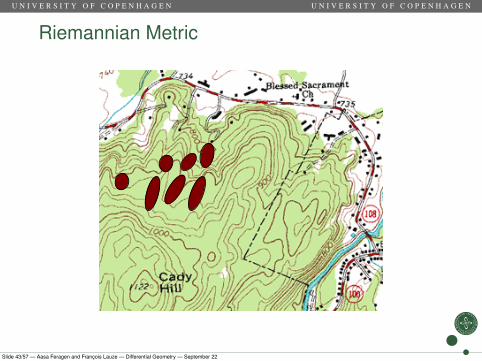
Why do we care about nonlinearity?
• Nonlinear relations between data objects• True distances not reflected by linear representation
”Topographic map example”. Licensed under Public domain via Wikimedia Commons -http://commons.wikimedia.org/wiki/File:Topographic_map_example.png#mediaviewer/File:Topographic_map_example.png
Slide 5/57 — Aasa Feragen and François Lauze — Differential Geometry — September 22

U N I V E R S I T Y O F C O P E N H A G E N U N I V E R S I T Y O F C O P E N H A G E N
Mildly nonlinear: Nonlinear transformationsbetween different linear representations
• Kernels!• Feature map = nonlinear transformation of (linear?) data space
X into linear feature space H• Learning problem is (usually) linear in H, not in X .
Slide 6/57 — Aasa Feragen and François Lauze — Differential Geometry — September 22

U N I V E R S I T Y O F C O P E N H A G E N U N I V E R S I T Y O F C O P E N H A G E N
Mildly nonlinear: Nonlinearly embeddedsubspaces whose intrinsic metric is linear• Manifold learning!
• Find intrinsic dataset distances• Find an Rd embedding that minimally distorts those distances
• Searches for the folded-up Euclidean space that best fits thedata
• the embedding of the data in feature space is nonlinear• the recovered intrinsic distance structure is linear
Slide 7/57 — Aasa Feragen and François Lauze — Differential Geometry — September 22
U N I V E R S I T Y O F C O P E N H A G E N U N I V E R S I T Y O F C O P E N H A G E N
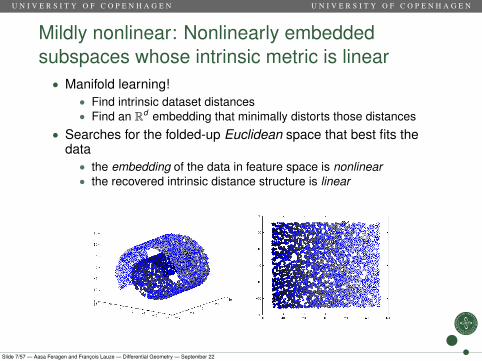
Mildly nonlinear: Nonlinearly embeddedsubspaces whose intrinsic metric is linear• Manifold learning!
• Find intrinsic dataset distances• Find an Rd embedding that minimally distorts those distances
• Searches for the folded-up Euclidean space that best fits thedata
• the embedding of the data in feature space is nonlinear• the recovered intrinsic distance structure is linear
Slide 7/57 — Aasa Feragen and François Lauze — Differential Geometry — September 22

U N I V E R S I T Y O F C O P E N H A G E N U N I V E R S I T Y O F C O P E N H A G E N
More nonlinear: Data spaces which areintrinsically nonlinear
• Distances distorted in nonlinear way, varying spatially• We shall see: the distances cannot always be linearized
”Topographic map example”. Licensed under Public domain via Wikimedia Commons -http://commons.wikimedia.org/wiki/File:Topographic_map_example.png#mediaviewer/File:Topographic_map_example.png
Slide 8/57 — Aasa Feragen and François Lauze — Differential Geometry — September 22
U N I V E R S I T Y O F C O P E N H A G E N U N I V E R S I T Y O F C O P E N H A G E N
Intrinsically nonlinear data spaces:Smooth manifolds
DefinitionA manifold is a set M with an associated one-to-one map ϕ : U → Mfrom an open subset U ⊂ Rm called a global chart or a globalcoordinate system for M.
• Open set U ⊂ Rm = set that does not contain its boundary• Manifold M gets its topology (= definition of open sets) from U
via ϕ• What are the implications of getting the topology from U?
Slide 9/57 — Aasa Feragen and François Lauze — Differential Geometry — September 22

U N I V E R S I T Y O F C O P E N H A G E N U N I V E R S I T Y O F C O P E N H A G E N
Intrinsically nonlinear data spaces:Smooth manifolds
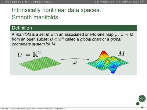
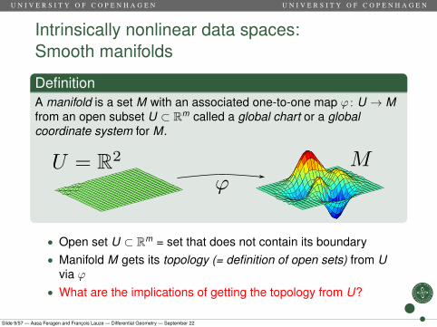
DefinitionA manifold is a set M with an associated one-to-one map ϕ : U → Mfrom an open subset U ⊂ Rm called a global chart or a globalcoordinate system for M.
• Open set U ⊂ Rm = set that does not contain its boundary• Manifold M gets its topology (= definition of open sets) from U
via ϕ
• What are the implications of getting the topology from U?
Slide 9/57 — Aasa Feragen and François Lauze — Differential Geometry — September 22
U N I V E R S I T Y O F C O P E N H A G E N U N I V E R S I T Y O F C O P E N H A G E N
Intrinsically nonlinear data spaces:Smooth manifolds
DefinitionA manifold is a set M with an associated one-to-one map ϕ : U → Mfrom an open subset U ⊂ Rm called a global chart or a globalcoordinate system for M.
• Open set U ⊂ Rm = set that does not contain its boundary• Manifold M gets its topology (= definition of open sets) from U
via ϕ• What are the implications of getting the topology from U?
Slide 9/57 — Aasa Feragen and François Lauze — Differential Geometry — September 22
U N I V E R S I T Y O F C O P E N H A G E N U N I V E R S I T Y O F C O P E N H A G E N
Intrinsically nonlinear data spaces:Smooth manifolds
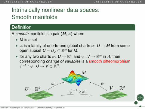
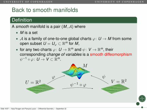
DefinitionA smooth manifold is a pair (M,A) where• M is a set• A is a family of one-to-one global charts ϕ : U → M from some
open subset U = Uϕ ⊂ Rm for M,• for any two charts ϕ : U → Rm and ψ : V → Rm in A, their
corresponding change of variables is a smooth diffeomorphismψ−1 ◦ ϕ : U → V ⊂ Rm.
Slide 9/57 — Aasa Feragen and François Lauze — Differential Geometry — September 22

U N I V E R S I T Y O F C O P E N H A G E N U N I V E R S I T Y O F C O P E N H A G E N
Outline
1 MotivationNonlinearityRecall: Calculus in Rn
2 Differential GeometrySmooth manifoldsBuilding ManifoldsTangent SpaceVector fieldsDifferential of smooth map
3 Riemannian metricsIntroduction to Riemannian metricsRecall: Inner ProductsRiemannian metricsInvariance of the Fisher information metricA first take on the geodesic distance metricA first take on curvature
Slide 10/57 — Aasa Feragen and François Lauze — Differential Geometry — September 22
U N I V E R S I T Y O F C O P E N H A G E N U N I V E R S I T Y O F C O P E N H A G E N
Differentiable and smooth functions
• f : U open ⊂ Rn → Rq continuous: write
(y1, . . . , yq) = f (x1, . . . , xn)
• f is of class Cr if f has continuous partial derivatives
∂r1+···+rn yk
∂x r11 . . . ∂x rn
n
k = 1 . . . q, r1 + . . . rn ≤ r .• When r =∞, f is smooth. Our focus.
Slide 11/57 — Aasa Feragen and François Lauze — Differential Geometry — September 22
U N I V E R S I T Y O F C O P E N H A G E N U N I V E R S I T Y O F C O P E N H A G E N
Differentiable and smooth functions
• f : U open ⊂ Rn → Rq continuous: write
(y1, . . . , yq) = f (x1, . . . , xn)
• f is of class Cr if f has continuous partial derivatives
∂r1+···+rn yk
∂x r11 . . . ∂x rn
n
k = 1 . . . q, r1 + . . . rn ≤ r .
• When r =∞, f is smooth. Our focus.
Slide 11/57 — Aasa Feragen and François Lauze — Differential Geometry — September 22

U N I V E R S I T Y O F C O P E N H A G E N U N I V E R S I T Y O F C O P E N H A G E N
Differentiable and smooth functions
• f : U open ⊂ Rn → Rq continuous: write
(y1, . . . , yq) = f (x1, . . . , xn)
• f is of class Cr if f has continuous partial derivatives
∂r1+···+rn yk
∂x r11 . . . ∂x rn
n
k = 1 . . . q, r1 + . . . rn ≤ r .• When r =∞, f is smooth. Our focus.
Slide 11/57 — Aasa Feragen and François Lauze — Differential Geometry — September 22

U N I V E R S I T Y O F C O P E N H A G E N U N I V E R S I T Y O F C O P E N H A G E N
Differential, Jacobian Matrix
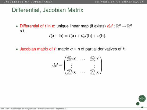
• Differential of f in x: unique linear map (if exists) dx f : Rn → Rq
s.t.f (x + h) = f (x) + dx f (h) + o(h).
• Jacobian matrix of f : matrix q × n of partial derivatives of f :
Jxf =
∂y1∂x1
(x) . . . ∂y1∂xn
(x)
......
∂yq∂x1
(x) . . .∂yq∂xn
(x)
• What is the meaning of the Jacobian? The differential? How do
they differ?
Slide 12/57 — Aasa Feragen and François Lauze — Differential Geometry — September 22
U N I V E R S I T Y O F C O P E N H A G E N U N I V E R S I T Y O F C O P E N H A G E N
Differential, Jacobian Matrix
• Differential of f in x: unique linear map (if exists) dx f : Rn → Rq
s.t.f (x + h) = f (x) + dx f (h) + o(h).
• Jacobian matrix of f : matrix q × n of partial derivatives of f :
Jxf =
∂y1∂x1
(x) . . . ∂y1∂xn
(x)
......
∂yq∂x1
(x) . . .∂yq∂xn
(x)
• What is the meaning of the Jacobian? The differential? How dothey differ?
Slide 12/57 — Aasa Feragen and François Lauze — Differential Geometry — September 22

U N I V E R S I T Y O F C O P E N H A G E N U N I V E R S I T Y O F C O P E N H A G E N
Differential, Jacobian Matrix
• Differential of f in x: unique linear map (if exists) dx f : Rn → Rq
s.t.f (x + h) = f (x) + dx f (h) + o(h).
• Jacobian matrix of f : matrix q × n of partial derivatives of f :
Jxf =
∂y1∂x1
(x) . . . ∂y1∂xn
(x)
......
∂yq∂x1
(x) . . .∂yq∂xn
(x)
• What is the meaning of the Jacobian? The differential? How do
they differ?
Slide 12/57 — Aasa Feragen and François Lauze — Differential Geometry — September 22

U N I V E R S I T Y O F C O P E N H A G E N U N I V E R S I T Y O F C O P E N H A G E N
Diffeomorphism
• When n = q:• If f is 1-1, f and f−1 both Cr
• f is a Cr -diffeomorphism.• Smooth diffeomorphisms are simply referred to as a
diffeomorphisms.
• Inverse Function Theorem:• f diffeomorphism⇒ det(Jxf ) 6= 0.• det(Jxf ) 6= 0⇒ f local diffeomorphism in a neighborhood of x.
• What is the meaning of Jxf? Of det(Jxf ) 6= 0?
Slide 13/57 — Aasa Feragen and François Lauze — Differential Geometry — September 22

U N I V E R S I T Y O F C O P E N H A G E N U N I V E R S I T Y O F C O P E N H A G E N
Diffeomorphism
• When n = q:• If f is 1-1, f and f−1 both Cr
• f is a Cr -diffeomorphism.• Smooth diffeomorphisms are simply referred to as a
diffeomorphisms.• Inverse Function Theorem:
• f diffeomorphism⇒ det(Jxf ) 6= 0.• det(Jxf ) 6= 0⇒ f local diffeomorphism in a neighborhood of x.
• What is the meaning of Jxf? Of det(Jxf ) 6= 0?
Slide 13/57 — Aasa Feragen and François Lauze — Differential Geometry — September 22

U N I V E R S I T Y O F C O P E N H A G E N U N I V E R S I T Y O F C O P E N H A G E N
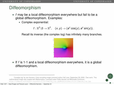
Diffeomorphism• f may be a local diffeomorphism everywhere but fail to be a
global diffeomorphism. Examples:• Complex exponential:
f : R2\0→ R2, (x , y)→ (ex cos(y), ex sin(y)).
Recall its inverse (the complex log) has infinitely many branches.
• If f is 1-1 and a local diffeomorphism everywhere, it is a globaldiffeomorphism.
• What is the intuitive meaning of a diffeomorphism?
”Complex log” by Jan Homann; Color encoding image comment author Hal Lane, September 28, 2009 - Own work. Thismathematical image was created with Mathematica. Licensed under Public domain via Wikimedia Commons -http://commons.wikimedia.org/wiki/File:Complex_log.jpg#mediaviewer/File:Complex_log.jpg
Slide 14/57 — Aasa Feragen and François Lauze — Differential Geometry — September 22
U N I V E R S I T Y O F C O P E N H A G E N U N I V E R S I T Y O F C O P E N H A G E N
Diffeomorphism• f may be a local diffeomorphism everywhere but fail to be a
global diffeomorphism. Examples:• Complex exponential:
f : R2\0→ R2, (x , y)→ (ex cos(y), ex sin(y)).
Recall its inverse (the complex log) has infinitely many branches.
• If f is 1-1 and a local diffeomorphism everywhere, it is a globaldiffeomorphism.
• What is the intuitive meaning of a diffeomorphism?
”Complex log” by Jan Homann; Color encoding image comment author Hal Lane, September 28, 2009 - Own work. Thismathematical image was created with Mathematica. Licensed under Public domain via Wikimedia Commons -http://commons.wikimedia.org/wiki/File:Complex_log.jpg#mediaviewer/File:Complex_log.jpg
Slide 14/57 — Aasa Feragen and François Lauze — Differential Geometry — September 22

U N I V E R S I T Y O F C O P E N H A G E N U N I V E R S I T Y O F C O P E N H A G E N
Outline
1 MotivationNonlinearityRecall: Calculus in Rn
2 Differential GeometrySmooth manifoldsBuilding ManifoldsTangent SpaceVector fieldsDifferential of smooth map
3 Riemannian metricsIntroduction to Riemannian metricsRecall: Inner ProductsRiemannian metricsInvariance of the Fisher information metricA first take on the geodesic distance metricA first take on curvature
Slide 15/57 — Aasa Feragen and François Lauze — Differential Geometry — September 22
U N I V E R S I T Y O F C O P E N H A G E N U N I V E R S I T Y O F C O P E N H A G E N
Back to smooth manifolds
DefinitionA smooth manifold is a pair (M,A) where• M is a set• A is a family of one-to-one global charts ϕ : U → M from some
open subset U = Uϕ ⊂ Rm for M,• for any two charts ϕ : U → Rm and ψ : V → Rm, their
corresponding change of variables is a smooth diffeomorphismψ−1 ◦ ϕ : U → V ⊂ Rm.
• What are the implications of inheriting structure through A?
Slide 16/57 — Aasa Feragen and François Lauze — Differential Geometry — September 22
U N I V E R S I T Y O F C O P E N H A G E N U N I V E R S I T Y O F C O P E N H A G E N
Back to smooth manifolds
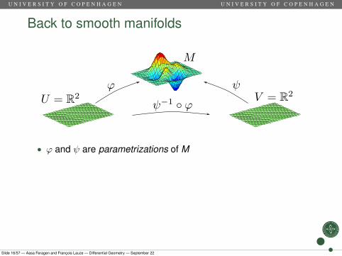
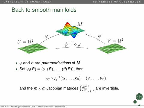
• ϕ and ψ are parametrizations of M
• Set ϕj (P) = (y1(P), . . . , yn(P)), then
ϕj ◦ ϕ−1i (x1, . . . , xm) = (y1, . . . , ym)
and the m ×m Jacobian matrices(∂yk
∂xh
)k,h
are invertible.
Slide 16/57 — Aasa Feragen and François Lauze — Differential Geometry — September 22
U N I V E R S I T Y O F C O P E N H A G E N U N I V E R S I T Y O F C O P E N H A G E N
Back to smooth manifolds
• ϕ and ψ are parametrizations of M• Set ϕj (P) = (y1(P), . . . , yn(P)), then
ϕj ◦ ϕ−1i (x1, . . . , xm) = (y1, . . . , ym)
and the m ×m Jacobian matrices(∂yk
∂xh
)k,h
are invertible.
Slide 16/57 — Aasa Feragen and François Lauze — Differential Geometry — September 22

U N I V E R S I T Y O F C O P E N H A G E N U N I V E R S I T Y O F C O P E N H A G E N
Example: Euclidean space
• The Euclidean space Rn is a manifold: take ϕ = Id as globalcoordinate system!
Slide 17/57 — Aasa Feragen and François Lauze — Differential Geometry — September 22

U N I V E R S I T Y O F C O P E N H A G E N U N I V E R S I T Y O F C O P E N H A G E N
Example: Smooth surfaces
• Smooth surfaces in Rn that are the image of a smooth mapf : R2 → Rn.
• A global coordinate system given by f
Slide 18/57 — Aasa Feragen and François Lauze — Differential Geometry — September 22

U N I V E R S I T Y O F C O P E N H A G E N U N I V E R S I T Y O F C O P E N H A G E N
Example: Symmetric Positive Definite Matrices• P(n) ⊂ GLn consists of all symmetric n × n matrices A that
satisfy
xAxT > 0 for any x ∈ Rn, (positive definite – PD – matrices)
• P(n) = the set of covariance matrices on Rn
• P(3) = the set of (diffusion) tensors on R3
• Global chart: P(n) is an open, convex subset of R(n2+n)/2
• A,B ∈ P(n)→ aA + bB ∈ P(n) for all a, b > 0 so P(n) is a convexcone in R(n2+n)/2.
Middle figure from Fillard et al., A Riemannian Framework for the Processing of Tensor-Valued Images, LNCS 3753, 2005, pp112-123. Rightmost figure from Fletcher, Joshi, Principal Geodesic Analysis on Symmetric Spaces: Statistics of Diffusion Tensors,CVAMIA04
Slide 19/57 — Aasa Feragen and François Lauze — Differential Geometry — September 22

U N I V E R S I T Y O F C O P E N H A G E N U N I V E R S I T Y O F C O P E N H A G E N
Example: Space of Gaussian distributions
• The space of n-dimensional Gaussian distributions is a smoothmanifold
• Global chart: (µ,Σ) ∈ Rn × P(n).
Slide 20/57 — Aasa Feragen and François Lauze — Differential Geometry — September 22
U N I V E R S I T Y O F C O P E N H A G E N U N I V E R S I T Y O F C O P E N H A G E N
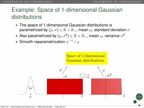
Example: Space of 1-dimensional Gaussiandistributions• The space of 1-dimensional Gaussian distributions is
parametrized by (µ, σ) ∈ R× R+, mean µ, standard deviation σ• Also parametrized by (µ, σ2) ∈ R× R+, mean µ, variance σ2
• Smooth reparametrization ψ−1 ◦ ϕ
Slide 21/57 — Aasa Feragen and François Lauze — Differential Geometry — September 22

U N I V E R S I T Y O F C O P E N H A G E N U N I V E R S I T Y O F C O P E N H A G E N
In general: Manifolds requiring multiple charts
The sphere S2 = {(x , y , z), x2 + y2 + z2 = 1}
For instance the projection from North Pole, given, for a pointP = (x , y , z) 6= N of the sphere, by
ϕN(P) =
(x
1− z,
y1− z
)is a (large) local coordinate system (around the south pole).
In these cases, we also require the charts to overlap ”nicely”
Slide 22/57 — Aasa Feragen and François Lauze — Differential Geometry — September 22

U N I V E R S I T Y O F C O P E N H A G E N U N I V E R S I T Y O F C O P E N H A G E N
In general: Manifolds requiring multiple charts
The Moebius strip
u ∈ [0,2π], v ∈ [12,
12
]
cos(u)(1 + 1
2 v cos( u2 ))
sin(u)(1 + 1
2 v cos( u2 ))
12 v sin( u
2 )
The 2D-torus
(u, v) ∈ [0,2π]2,R � r > 0cos(u) (R + r cos(v))sin(u) (R + r cos(v))
r sin(v)
Slide 22/57 — Aasa Feragen and François Lauze — Differential Geometry — September 22

U N I V E R S I T Y O F C O P E N H A G E N U N I V E R S I T Y O F C O P E N H A G E N
Smooth maps between manifolds
• f : M → N is smooth if its expression in any global coordinatesfor M and N is.
• ϕ global coordinates for M, ψ global coordinates for N
ϕ−1 ◦ f ◦ ψ smooth.
Slide 23/57 — Aasa Feragen and François Lauze — Differential Geometry — September 22
U N I V E R S I T Y O F C O P E N H A G E N U N I V E R S I T Y O F C O P E N H A G E N
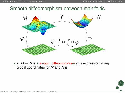
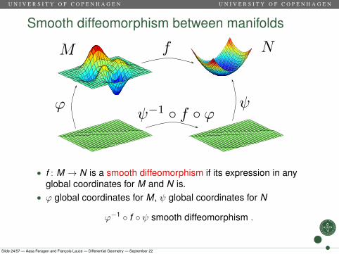
Smooth diffeomorphism between manifolds
• f : M → N is a smooth diffeomorphism if its expression in anyglobal coordinates for M and N is.
• ϕ global coordinates for M, ψ global coordinates for N
ϕ−1 ◦ f ◦ ψ smooth diffeomorphism .
Slide 24/57 — Aasa Feragen and François Lauze — Differential Geometry — September 22

U N I V E R S I T Y O F C O P E N H A G E N U N I V E R S I T Y O F C O P E N H A G E N
Smooth diffeomorphism between manifolds
• f : M → N is a smooth diffeomorphism if its expression in anyglobal coordinates for M and N is.
• ϕ global coordinates for M, ψ global coordinates for N
ϕ−1 ◦ f ◦ ψ smooth diffeomorphism .
Slide 24/57 — Aasa Feragen and François Lauze — Differential Geometry — September 22

U N I V E R S I T Y O F C O P E N H A G E N U N I V E R S I T Y O F C O P E N H A G E N
Outline
1 MotivationNonlinearityRecall: Calculus in Rn
2 Differential GeometrySmooth manifoldsBuilding ManifoldsTangent SpaceVector fieldsDifferential of smooth map
3 Riemannian metricsIntroduction to Riemannian metricsRecall: Inner ProductsRiemannian metricsInvariance of the Fisher information metricA first take on the geodesic distance metricA first take on curvature
Slide 25/57 — Aasa Feragen and François Lauze — Differential Geometry — September 22

U N I V E R S I T Y O F C O P E N H A G E N U N I V E R S I T Y O F C O P E N H A G E N
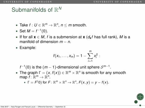
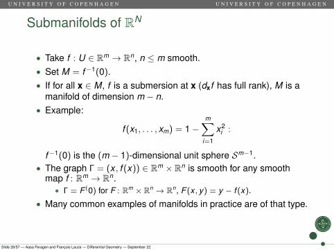
Submanifolds of RN
• Take f : U ∈ Rm → Rn, n ≤ m smooth.
• Set M = f−1(0).• If for all x ∈ M, f is a submersion at x (dxf has full rank), M is a
manifold of dimension m − n.• Example:
f (x1, . . . , xm) = 1−m∑
i=1
x2i :
f−1(0) is the (m − 1)-dimensional unit sphere Sm−1.• The graph Γ = (x , f (x)) ∈ Rm × Rn is smooth for any smooth
map f : Rm → Rn.
• Γ = F (0) for F : Rm × Rn → Rn, F (x , y) = y − f (x).
• Many common examples of manifolds in practice are of that type.
Slide 26/57 — Aasa Feragen and François Lauze — Differential Geometry — September 22

U N I V E R S I T Y O F C O P E N H A G E N U N I V E R S I T Y O F C O P E N H A G E N
Submanifolds of RN
• Take f : U ∈ Rm → Rn, n ≤ m smooth.• Set M = f−1(0).
• If for all x ∈ M, f is a submersion at x (dxf has full rank), M is amanifold of dimension m − n.
• Example:
f (x1, . . . , xm) = 1−m∑
i=1
x2i :
f−1(0) is the (m − 1)-dimensional unit sphere Sm−1.• The graph Γ = (x , f (x)) ∈ Rm × Rn is smooth for any smooth
map f : Rm → Rn.
• Γ = F (0) for F : Rm × Rn → Rn, F (x , y) = y − f (x).
• Many common examples of manifolds in practice are of that type.
Slide 26/57 — Aasa Feragen and François Lauze — Differential Geometry — September 22

U N I V E R S I T Y O F C O P E N H A G E N U N I V E R S I T Y O F C O P E N H A G E N
Submanifolds of RN
• Take f : U ∈ Rm → Rn, n ≤ m smooth.• Set M = f−1(0).• If for all x ∈ M, f is a submersion at x (dxf has full rank), M is a
manifold of dimension m − n.
• Example:
f (x1, . . . , xm) = 1−m∑
i=1
x2i :
f−1(0) is the (m − 1)-dimensional unit sphere Sm−1.• The graph Γ = (x , f (x)) ∈ Rm × Rn is smooth for any smooth
map f : Rm → Rn.
• Γ = F (0) for F : Rm × Rn → Rn, F (x , y) = y − f (x).
• Many common examples of manifolds in practice are of that type.
Slide 26/57 — Aasa Feragen and François Lauze — Differential Geometry — September 22

U N I V E R S I T Y O F C O P E N H A G E N U N I V E R S I T Y O F C O P E N H A G E N
Submanifolds of RN
• Take f : U ∈ Rm → Rn, n ≤ m smooth.• Set M = f−1(0).• If for all x ∈ M, f is a submersion at x (dxf has full rank), M is a
manifold of dimension m − n.• Example:
f (x1, . . . , xm) = 1−m∑
i=1
x2i :
f−1(0) is the (m − 1)-dimensional unit sphere Sm−1.
• The graph Γ = (x , f (x)) ∈ Rm × Rn is smooth for any smoothmap f : Rm → Rn.
• Γ = F (0) for F : Rm × Rn → Rn, F (x , y) = y − f (x).
• Many common examples of manifolds in practice are of that type.
Slide 26/57 — Aasa Feragen and François Lauze — Differential Geometry — September 22

U N I V E R S I T Y O F C O P E N H A G E N U N I V E R S I T Y O F C O P E N H A G E N
Submanifolds of RN
• Take f : U ∈ Rm → Rn, n ≤ m smooth.• Set M = f−1(0).• If for all x ∈ M, f is a submersion at x (dxf has full rank), M is a
manifold of dimension m − n.• Example:
f (x1, . . . , xm) = 1−m∑
i=1
x2i :
f−1(0) is the (m − 1)-dimensional unit sphere Sm−1.• The graph Γ = (x , f (x)) ∈ Rm × Rn is smooth for any smooth
map f : Rm → Rn.
• Γ = F (0) for F : Rm × Rn → Rn, F (x , y) = y − f (x).
• Many common examples of manifolds in practice are of that type.
Slide 26/57 — Aasa Feragen and François Lauze — Differential Geometry — September 22
U N I V E R S I T Y O F C O P E N H A G E N U N I V E R S I T Y O F C O P E N H A G E N
Submanifolds of RN
• Take f : U ∈ Rm → Rn, n ≤ m smooth.• Set M = f−1(0).• If for all x ∈ M, f is a submersion at x (dxf has full rank), M is a
manifold of dimension m − n.• Example:
f (x1, . . . , xm) = 1−m∑
i=1
x2i :
f−1(0) is the (m − 1)-dimensional unit sphere Sm−1.• The graph Γ = (x , f (x)) ∈ Rm × Rn is smooth for any smooth
map f : Rm → Rn.• Γ = F (0) for F : Rm × Rn → Rn, F (x , y) = y − f (x).
• Many common examples of manifolds in practice are of that type.
Slide 26/57 — Aasa Feragen and François Lauze — Differential Geometry — September 22

U N I V E R S I T Y O F C O P E N H A G E N U N I V E R S I T Y O F C O P E N H A G E N
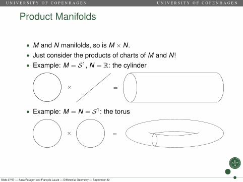
Product Manifolds
• M and N manifolds, so is M × N.
• Just consider the products of charts of M and N!• Example: M = S1, N = R: the cylinder
• Example: M = N = S1: the torus
Slide 27/57 — Aasa Feragen and François Lauze — Differential Geometry — September 22

U N I V E R S I T Y O F C O P E N H A G E N U N I V E R S I T Y O F C O P E N H A G E N
Product Manifolds
• M and N manifolds, so is M × N.• Just consider the products of charts of M and N!
• Example: M = S1, N = R: the cylinder
• Example: M = N = S1: the torus
Slide 27/57 — Aasa Feragen and François Lauze — Differential Geometry — September 22

U N I V E R S I T Y O F C O P E N H A G E N U N I V E R S I T Y O F C O P E N H A G E N
Product Manifolds
• M and N manifolds, so is M × N.• Just consider the products of charts of M and N!• Example: M = S1, N = R: the cylinder
• Example: M = N = S1: the torus
Slide 27/57 — Aasa Feragen and François Lauze — Differential Geometry — September 22
U N I V E R S I T Y O F C O P E N H A G E N U N I V E R S I T Y O F C O P E N H A G E N
Outline
1 MotivationNonlinearityRecall: Calculus in Rn
2 Differential GeometrySmooth manifoldsBuilding ManifoldsTangent SpaceVector fieldsDifferential of smooth map
3 Riemannian metricsIntroduction to Riemannian metricsRecall: Inner ProductsRiemannian metricsInvariance of the Fisher information metricA first take on the geodesic distance metricA first take on curvature
Slide 28/57 — Aasa Feragen and François Lauze — Differential Geometry — September 22
U N I V E R S I T Y O F C O P E N H A G E N U N I V E R S I T Y O F C O P E N H A G E N
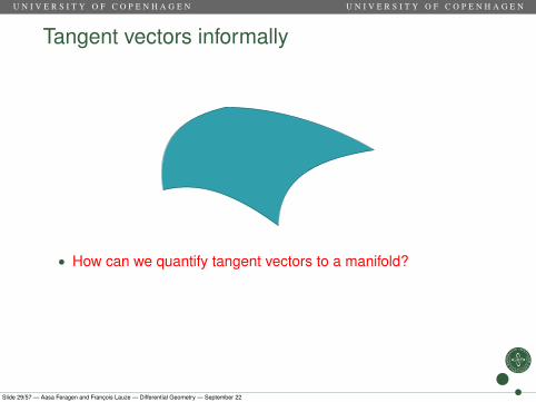
Tangent vectors informally
• How can we quantify tangent vectors to a manifold?
• Informally: a tangent vector at P ∈ M: draw a curvec : (−ε, ε)→ M, c(0) = P, then c(0) is a tangent vector.
Slide 29/57 — Aasa Feragen and François Lauze — Differential Geometry — September 22

U N I V E R S I T Y O F C O P E N H A G E N U N I V E R S I T Y O F C O P E N H A G E N
Tangent vectors informally
• How can we quantify tangent vectors to a manifold?• Informally: a tangent vector at P ∈ M: draw a curve
c : (−ε, ε)→ M, c(0) = P, then c(0) is a tangent vector.
Slide 29/57 — Aasa Feragen and François Lauze — Differential Geometry — September 22

U N I V E R S I T Y O F C O P E N H A G E N U N I V E R S I T Y O F C O P E N H A G E N
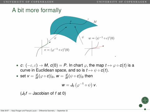
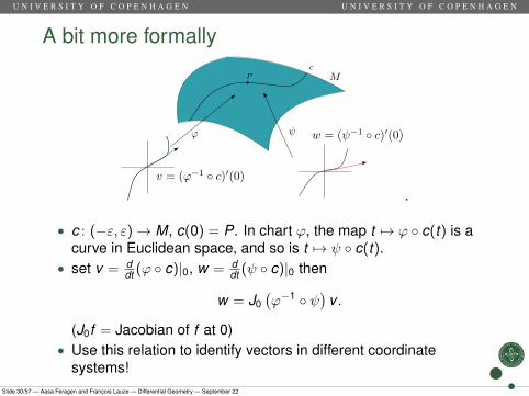
A bit more formally
.
• c : (−ε, ε)→ M, c(0) = P. In chart ϕ, the map t 7→ ϕ ◦ c(t) is acurve in Euclidean space, and so is t 7→ ψ ◦ c(t).
• set v = ddt (ϕ ◦ c)|0, w = d
dt (ψ ◦ c)|0 then
w = J0(ϕ−1 ◦ ψ
)v .
(J0f = Jacobian of f at 0)• Use this relation to identify vectors in different coordinate
systems!
Slide 30/57 — Aasa Feragen and François Lauze — Differential Geometry — September 22

U N I V E R S I T Y O F C O P E N H A G E N U N I V E R S I T Y O F C O P E N H A G E N
A bit more formally
.
• c : (−ε, ε)→ M, c(0) = P. In chart ϕ, the map t 7→ ϕ ◦ c(t) is acurve in Euclidean space, and so is t 7→ ψ ◦ c(t).
• set v = ddt (ϕ ◦ c)|0, w = d
dt (ψ ◦ c)|0 then
w = J0(ϕ−1 ◦ ψ
)v .
(J0f = Jacobian of f at 0)• Use this relation to identify vectors in different coordinate
systems!
Slide 30/57 — Aasa Feragen and François Lauze — Differential Geometry — September 22
U N I V E R S I T Y O F C O P E N H A G E N U N I V E R S I T Y O F C O P E N H A G E N
A bit more formally
.
• c : (−ε, ε)→ M, c(0) = P. In chart ϕ, the map t 7→ ϕ ◦ c(t) is acurve in Euclidean space, and so is t 7→ ψ ◦ c(t).
• set v = ddt (ϕ ◦ c)|0, w = d
dt (ψ ◦ c)|0 then
w = J0(ϕ−1 ◦ ψ
)v .
(J0f = Jacobian of f at 0)
• Use this relation to identify vectors in different coordinatesystems!
Slide 30/57 — Aasa Feragen and François Lauze — Differential Geometry — September 22
U N I V E R S I T Y O F C O P E N H A G E N U N I V E R S I T Y O F C O P E N H A G E N
A bit more formally
.
• c : (−ε, ε)→ M, c(0) = P. In chart ϕ, the map t 7→ ϕ ◦ c(t) is acurve in Euclidean space, and so is t 7→ ψ ◦ c(t).
• set v = ddt (ϕ ◦ c)|0, w = d
dt (ψ ◦ c)|0 then
w = J0(ϕ−1 ◦ ψ
)v .
(J0f = Jacobian of f at 0)• Use this relation to identify vectors in different coordinate
systems!Slide 30/57 — Aasa Feragen and François Lauze — Differential Geometry — September 22

U N I V E R S I T Y O F C O P E N H A G E N U N I V E R S I T Y O F C O P E N H A G E N
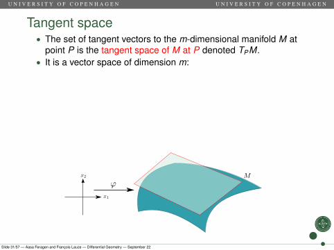
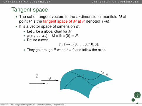
Tangent space• The set of tangent vectors to the m-dimensional manifold M at
point P is the tangent space of M at P denoted TPM.
• It is a vector space of dimension m:
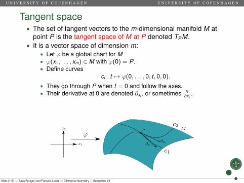
• Let ϕ be a global chart for M• ϕ(x1, . . . , xm) ∈ M with ϕ(0) = P.• Define curves
ci : t 7→ ϕ(0, . . . , 0, t , 0, 0).
• They go through P when t = 0 and follow the axes.• Their derivative at 0 are denoted ∂xi , or sometimes ∂
∂xi.
• The ∂xi form a basis of TPM.
Slide 31/57 — Aasa Feragen and François Lauze — Differential Geometry — September 22
U N I V E R S I T Y O F C O P E N H A G E N U N I V E R S I T Y O F C O P E N H A G E N
Tangent space• The set of tangent vectors to the m-dimensional manifold M at
point P is the tangent space of M at P denoted TPM.• It is a vector space of dimension m:
• Let ϕ be a global chart for M• ϕ(x1, . . . , xm) ∈ M with ϕ(0) = P.• Define curves
ci : t 7→ ϕ(0, . . . , 0, t , 0, 0).
• They go through P when t = 0 and follow the axes.• Their derivative at 0 are denoted ∂xi , or sometimes ∂
∂xi.
• The ∂xi form a basis of TPM.
Slide 31/57 — Aasa Feragen and François Lauze — Differential Geometry — September 22

U N I V E R S I T Y O F C O P E N H A G E N U N I V E R S I T Y O F C O P E N H A G E N
Tangent space• The set of tangent vectors to the m-dimensional manifold M at
point P is the tangent space of M at P denoted TPM.• It is a vector space of dimension m:
• Let ϕ be a global chart for M
• ϕ(x1, . . . , xm) ∈ M with ϕ(0) = P.• Define curves
ci : t 7→ ϕ(0, . . . , 0, t , 0, 0).
• They go through P when t = 0 and follow the axes.• Their derivative at 0 are denoted ∂xi , or sometimes ∂
∂xi.
• The ∂xi form a basis of TPM.
Slide 31/57 — Aasa Feragen and François Lauze — Differential Geometry — September 22

U N I V E R S I T Y O F C O P E N H A G E N U N I V E R S I T Y O F C O P E N H A G E N
Tangent space• The set of tangent vectors to the m-dimensional manifold M at
point P is the tangent space of M at P denoted TPM.• It is a vector space of dimension m:
• Let ϕ be a global chart for M• ϕ(x1, . . . , xm) ∈ M with ϕ(0) = P.
• Define curvesci : t 7→ ϕ(0, . . . , 0, t , 0, 0).
• They go through P when t = 0 and follow the axes.• Their derivative at 0 are denoted ∂xi , or sometimes ∂
∂xi.
• The ∂xi form a basis of TPM.
Slide 31/57 — Aasa Feragen and François Lauze — Differential Geometry — September 22

U N I V E R S I T Y O F C O P E N H A G E N U N I V E R S I T Y O F C O P E N H A G E N
Tangent space• The set of tangent vectors to the m-dimensional manifold M at
point P is the tangent space of M at P denoted TPM.• It is a vector space of dimension m:
• Let ϕ be a global chart for M• ϕ(x1, . . . , xm) ∈ M with ϕ(0) = P.• Define curves
ci : t 7→ ϕ(0, . . . , 0, t , 0, 0).
• They go through P when t = 0 and follow the axes.• Their derivative at 0 are denoted ∂xi , or sometimes ∂
∂xi.
• The ∂xi form a basis of TPM.
Slide 31/57 — Aasa Feragen and François Lauze — Differential Geometry — September 22
U N I V E R S I T Y O F C O P E N H A G E N U N I V E R S I T Y O F C O P E N H A G E N
Tangent space• The set of tangent vectors to the m-dimensional manifold M at
point P is the tangent space of M at P denoted TPM.• It is a vector space of dimension m:
• Let ϕ be a global chart for M• ϕ(x1, . . . , xm) ∈ M with ϕ(0) = P.• Define curves
ci : t 7→ ϕ(0, . . . , 0, t , 0, 0).
• They go through P when t = 0 and follow the axes.
• Their derivative at 0 are denoted ∂xi , or sometimes ∂∂xi
.• The ∂xi form a basis of TPM.
Slide 31/57 — Aasa Feragen and François Lauze — Differential Geometry — September 22
U N I V E R S I T Y O F C O P E N H A G E N U N I V E R S I T Y O F C O P E N H A G E N
Tangent space• The set of tangent vectors to the m-dimensional manifold M at
point P is the tangent space of M at P denoted TPM.• It is a vector space of dimension m:
• Let ϕ be a global chart for M• ϕ(x1, . . . , xm) ∈ M with ϕ(0) = P.• Define curves
ci : t 7→ ϕ(0, . . . , 0, t , 0, 0).
• They go through P when t = 0 and follow the axes.• Their derivative at 0 are denoted ∂xi , or sometimes ∂
∂xi.
• The ∂xi form a basis of TPM.
Slide 31/57 — Aasa Feragen and François Lauze — Differential Geometry — September 22
U N I V E R S I T Y O F C O P E N H A G E N U N I V E R S I T Y O F C O P E N H A G E N
Outline
1 MotivationNonlinearityRecall: Calculus in Rn
2 Differential GeometrySmooth manifoldsBuilding ManifoldsTangent SpaceVector fieldsDifferential of smooth map
3 Riemannian metricsIntroduction to Riemannian metricsRecall: Inner ProductsRiemannian metricsInvariance of the Fisher information metricA first take on the geodesic distance metricA first take on curvature
Slide 32/57 — Aasa Feragen and François Lauze — Differential Geometry — September 22

U N I V E R S I T Y O F C O P E N H A G E N U N I V E R S I T Y O F C O P E N H A G E N
Vector fields
• A vector field is a smooth map that sends P ∈ M to a vectorv(P) ∈ TPM.
Slide 33/57 — Aasa Feragen and François Lauze — Differential Geometry — September 22
U N I V E R S I T Y O F C O P E N H A G E N U N I V E R S I T Y O F C O P E N H A G E N
Outline
1 MotivationNonlinearityRecall: Calculus in Rn
2 Differential GeometrySmooth manifoldsBuilding ManifoldsTangent SpaceVector fieldsDifferential of smooth map
3 Riemannian metricsIntroduction to Riemannian metricsRecall: Inner ProductsRiemannian metricsInvariance of the Fisher information metricA first take on the geodesic distance metricA first take on curvature
Slide 34/57 — Aasa Feragen and François Lauze — Differential Geometry — September 22

U N I V E R S I T Y O F C O P E N H A G E N U N I V E R S I T Y O F C O P E N H A G E N
Differential of a smooth map
• f : M → N smooth, P ∈ M, f (P) ∈ N
• dP f : TPM → Tf (P)N linear map corresponding to the Jacobianmatrix of f in local coordinates.
• When N = R, dP f is a linear form TPM → R.
Slide 35/57 — Aasa Feragen and François Lauze — Differential Geometry — September 22
U N I V E R S I T Y O F C O P E N H A G E N U N I V E R S I T Y O F C O P E N H A G E N
Differential of a smooth map
• f : M → N smooth, P ∈ M, f (P) ∈ N• dP f : TPM → Tf (P)N linear map corresponding to the Jacobian
matrix of f in local coordinates.
• When N = R, dP f is a linear form TPM → R.
Slide 35/57 — Aasa Feragen and François Lauze — Differential Geometry — September 22

U N I V E R S I T Y O F C O P E N H A G E N U N I V E R S I T Y O F C O P E N H A G E N
Differential of a smooth map
• f : M → N smooth, P ∈ M, f (P) ∈ N• dP f : TPM → Tf (P)N linear map corresponding to the Jacobian
matrix of f in local coordinates.• When N = R, dP f is a linear form TPM → R.
Slide 35/57 — Aasa Feragen and François Lauze — Differential Geometry — September 22
U N I V E R S I T Y O F C O P E N H A G E N U N I V E R S I T Y O F C O P E N H A G E N
Outline
1 MotivationNonlinearityRecall: Calculus in Rn
2 Differential GeometrySmooth manifoldsBuilding ManifoldsTangent SpaceVector fieldsDifferential of smooth map
3 Riemannian metricsIntroduction to Riemannian metricsRecall: Inner ProductsRiemannian metricsInvariance of the Fisher information metricA first take on the geodesic distance metricA first take on curvature
Slide 36/57 — Aasa Feragen and François Lauze — Differential Geometry — September 22

U N I V E R S I T Y O F C O P E N H A G E N U N I V E R S I T Y O F C O P E N H A G E N
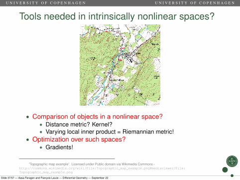
Tools needed in intrinsically nonlinear spaces?
• Comparison of objects in a nonlinear space?
• Distance metric? Kernel?• Varying local inner product = Riemannian metric!
• Optimization over such spaces?
• Gradients!
• Riemannian geometry
”Topographic map example”. Licensed under Public domain via Wikimedia Commons -http://commons.wikimedia.org/wiki/File:Topographic_map_example.png#mediaviewer/File:Topographic_map_example.png
Slide 37/57 — Aasa Feragen and François Lauze — Differential Geometry — September 22

U N I V E R S I T Y O F C O P E N H A G E N U N I V E R S I T Y O F C O P E N H A G E N
Tools needed in intrinsically nonlinear spaces?
• Comparison of objects in a nonlinear space?• Distance metric? Kernel?• Varying local inner product = Riemannian metric!
• Optimization over such spaces?
• Gradients!
• Riemannian geometry
”Topographic map example”. Licensed under Public domain via Wikimedia Commons -http://commons.wikimedia.org/wiki/File:Topographic_map_example.png#mediaviewer/File:Topographic_map_example.png
Slide 37/57 — Aasa Feragen and François Lauze — Differential Geometry — September 22

U N I V E R S I T Y O F C O P E N H A G E N U N I V E R S I T Y O F C O P E N H A G E N
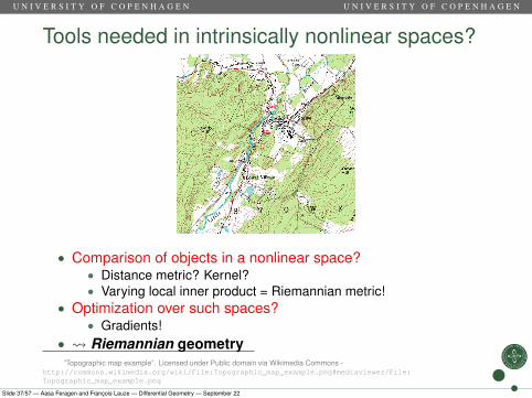
Tools needed in intrinsically nonlinear spaces?
• Comparison of objects in a nonlinear space?• Distance metric? Kernel?• Varying local inner product = Riemannian metric!
• Optimization over such spaces?
• Gradients!• Riemannian geometry
”Topographic map example”. Licensed under Public domain via Wikimedia Commons -http://commons.wikimedia.org/wiki/File:Topographic_map_example.png#mediaviewer/File:Topographic_map_example.png
Slide 37/57 — Aasa Feragen and François Lauze — Differential Geometry — September 22
U N I V E R S I T Y O F C O P E N H A G E N U N I V E R S I T Y O F C O P E N H A G E N
Tools needed in intrinsically nonlinear spaces?
• Comparison of objects in a nonlinear space?• Distance metric? Kernel?• Varying local inner product = Riemannian metric!
• Optimization over such spaces?• Gradients!
• Riemannian geometry
”Topographic map example”. Licensed under Public domain via Wikimedia Commons -http://commons.wikimedia.org/wiki/File:Topographic_map_example.png#mediaviewer/File:Topographic_map_example.png
Slide 37/57 — Aasa Feragen and François Lauze — Differential Geometry — September 22
U N I V E R S I T Y O F C O P E N H A G E N U N I V E R S I T Y O F C O P E N H A G E N
Tools needed in intrinsically nonlinear spaces?
• Comparison of objects in a nonlinear space?• Distance metric? Kernel?• Varying local inner product = Riemannian metric!
• Optimization over such spaces?• Gradients!
• Riemannian geometry”Topographic map example”. Licensed under Public domain via Wikimedia Commons -
http://commons.wikimedia.org/wiki/File:Topographic_map_example.png#mediaviewer/File:Topographic_map_example.png
Slide 37/57 — Aasa Feragen and François Lauze — Differential Geometry — September 22
U N I V E R S I T Y O F C O P E N H A G E N U N I V E R S I T Y O F C O P E N H A G E N
Outline
1 MotivationNonlinearityRecall: Calculus in Rn
2 Differential GeometrySmooth manifoldsBuilding ManifoldsTangent SpaceVector fieldsDifferential of smooth map
3 Riemannian metricsIntroduction to Riemannian metricsRecall: Inner ProductsRiemannian metricsInvariance of the Fisher information metricA first take on the geodesic distance metricA first take on curvature
Slide 38/57 — Aasa Feragen and François Lauze — Differential Geometry — September 22

U N I V E R S I T Y O F C O P E N H A G E N U N I V E R S I T Y O F C O P E N H A G E N
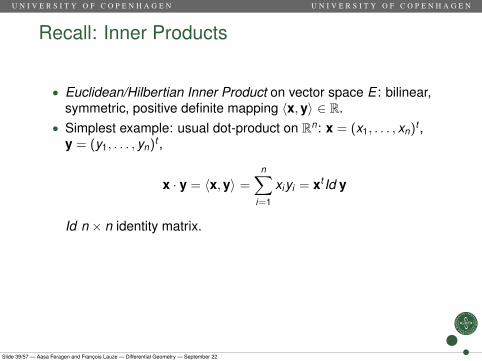
Recall: Inner Products
• Euclidean/Hilbertian Inner Product on vector space E : bilinear,symmetric, positive definite mapping 〈x,y〉 ∈ R.
• Simplest example: usual dot-product on Rn: x = (x1, . . . , xn)t ,y = (y1, . . . , yn)t ,
x · y = 〈x,y〉 =n∑
i=1
xiyi = xt Id y
Id n × n identity matrix.• xT Ay, A symmetric, positive definite: inner product, 〈x,y〉A.• Without subscript 〈−,−〉 will denote standard Euclidean
dot-product (i.e. A = Id).
Slide 39/57 — Aasa Feragen and François Lauze — Differential Geometry — September 22
U N I V E R S I T Y O F C O P E N H A G E N U N I V E R S I T Y O F C O P E N H A G E N
Recall: Inner Products
• Euclidean/Hilbertian Inner Product on vector space E : bilinear,symmetric, positive definite mapping 〈x,y〉 ∈ R.
• Simplest example: usual dot-product on Rn: x = (x1, . . . , xn)t ,y = (y1, . . . , yn)t ,
x · y = 〈x,y〉 =n∑
i=1
xiyi = xt Id y
Id n × n identity matrix.
• xT Ay, A symmetric, positive definite: inner product, 〈x,y〉A.• Without subscript 〈−,−〉 will denote standard Euclidean
dot-product (i.e. A = Id).
Slide 39/57 — Aasa Feragen and François Lauze — Differential Geometry — September 22

U N I V E R S I T Y O F C O P E N H A G E N U N I V E R S I T Y O F C O P E N H A G E N
Recall: Inner Products
• Euclidean/Hilbertian Inner Product on vector space E : bilinear,symmetric, positive definite mapping 〈x,y〉 ∈ R.
• Simplest example: usual dot-product on Rn: x = (x1, . . . , xn)t ,y = (y1, . . . , yn)t ,
x · y = 〈x,y〉 =n∑
i=1
xiyi = xt Id y
Id n × n identity matrix.• xT Ay, A symmetric, positive definite: inner product, 〈x,y〉A.
• Without subscript 〈−,−〉 will denote standard Euclideandot-product (i.e. A = Id).
Slide 39/57 — Aasa Feragen and François Lauze — Differential Geometry — September 22

U N I V E R S I T Y O F C O P E N H A G E N U N I V E R S I T Y O F C O P E N H A G E N
Recall: Inner Products
• Euclidean/Hilbertian Inner Product on vector space E : bilinear,symmetric, positive definite mapping 〈x,y〉 ∈ R.
• Simplest example: usual dot-product on Rn: x = (x1, . . . , xn)t ,y = (y1, . . . , yn)t ,
x · y = 〈x,y〉 =n∑
i=1
xiyi = xt Id y
Id n × n identity matrix.• xT Ay, A symmetric, positive definite: inner product, 〈x,y〉A.• Without subscript 〈−,−〉 will denote standard Euclidean
dot-product (i.e. A = Id).
Slide 39/57 — Aasa Feragen and François Lauze — Differential Geometry — September 22

U N I V E R S I T Y O F C O P E N H A G E N U N I V E R S I T Y O F C O P E N H A G E N
Orthogonality – Norm – Distance
• Orthogonality, vector norm, distance from inner products.
x⊥Ay ⇐⇒ 〈x,y〉A = 0, ‖x‖2A = 〈x,x〉A , dA(x,y) = ‖x− y‖A.
• � There are norms and distances not from an inner product.
Slide 40/57 — Aasa Feragen and François Lauze — Differential Geometry — September 22
U N I V E R S I T Y O F C O P E N H A G E N U N I V E R S I T Y O F C O P E N H A G E N
Inner Products and Duality
Linear form h = (h1, . . . ,hn) : Rn → R: h(x) =∑n
i=1 hixi .• inner product 〈−,−〉A on Rn: h represented by a unique vector
hA s.th(x) = 〈hA,x〉A
hA is the dual of h (w.r.t 〈−,−〉A).
• for standard dot product:
h =
h1...
hn
= hT !
• for general inner product 〈−,−〉A
hA = A−1h = A−1hT .
Slide 41/57 — Aasa Feragen and François Lauze — Differential Geometry — September 22

U N I V E R S I T Y O F C O P E N H A G E N U N I V E R S I T Y O F C O P E N H A G E N
Inner Products and Duality
Linear form h = (h1, . . . ,hn) : Rn → R: h(x) =∑n
i=1 hixi .• inner product 〈−,−〉A on Rn: h represented by a unique vector
hA s.th(x) = 〈hA,x〉A
hA is the dual of h (w.r.t 〈−,−〉A).• for standard dot product:
h =
h1...
hn
= hT !
• for general inner product 〈−,−〉A
hA = A−1h = A−1hT .
Slide 41/57 — Aasa Feragen and François Lauze — Differential Geometry — September 22

U N I V E R S I T Y O F C O P E N H A G E N U N I V E R S I T Y O F C O P E N H A G E N
Outline
1 MotivationNonlinearityRecall: Calculus in Rn
2 Differential GeometrySmooth manifoldsBuilding ManifoldsTangent SpaceVector fieldsDifferential of smooth map
3 Riemannian metricsIntroduction to Riemannian metricsRecall: Inner ProductsRiemannian metricsInvariance of the Fisher information metricA first take on the geodesic distance metricA first take on curvature
Slide 42/57 — Aasa Feragen and François Lauze — Differential Geometry — September 22

U N I V E R S I T Y O F C O P E N H A G E N U N I V E R S I T Y O F C O P E N H A G E N
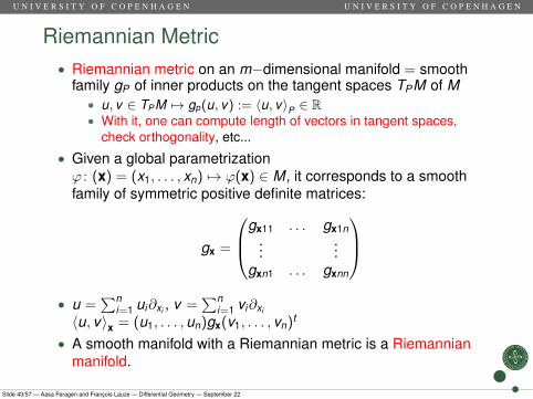
Riemannian Metric• Riemannian metric on an m−dimensional manifold = smooth
family gP of inner products on the tangent spaces TPM of M• u, v ∈ TPM 7→ gp(u, v) := 〈u, v〉P ∈ R• With it, one can compute length of vectors in tangent spaces,
check orthogonality, etc...
• Given a global parametrizationϕ : (x) = (x1, . . . , xn) 7→ ϕ(x) ∈ M, it corresponds to a smoothfamily of symmetric positive definite matrices:
gx =
gx11 . . . gx1n...
...gxn1 . . . gxnn
• u =
∑ni=1 ui∂xi , v =
∑ni=1 vi∂xi
〈u, v〉x = (u1, . . . ,un)gx(v1, . . . , vn)t
• A smooth manifold with a Riemannian metric is a Riemannianmanifold.
Slide 43/57 — Aasa Feragen and François Lauze — Differential Geometry — September 22

U N I V E R S I T Y O F C O P E N H A G E N U N I V E R S I T Y O F C O P E N H A G E N
Riemannian Metric• Riemannian metric on an m−dimensional manifold = smooth
family gP of inner products on the tangent spaces TPM of M• u, v ∈ TPM 7→ gp(u, v) := 〈u, v〉P ∈ R• With it, one can compute length of vectors in tangent spaces,
check orthogonality, etc...
• Given a global parametrizationϕ : (x) = (x1, . . . , xn) 7→ ϕ(x) ∈ M, it corresponds to a smoothfamily of symmetric positive definite matrices:
gx =
gx11 . . . gx1n...
...gxn1 . . . gxnn
• u =∑n
i=1 ui∂xi , v =∑n
i=1 vi∂xi
〈u, v〉x = (u1, . . . ,un)gx(v1, . . . , vn)t
• A smooth manifold with a Riemannian metric is a Riemannianmanifold.
Slide 43/57 — Aasa Feragen and François Lauze — Differential Geometry — September 22

U N I V E R S I T Y O F C O P E N H A G E N U N I V E R S I T Y O F C O P E N H A G E N
Riemannian Metric• Riemannian metric on an m−dimensional manifold = smooth
family gP of inner products on the tangent spaces TPM of M• u, v ∈ TPM 7→ gp(u, v) := 〈u, v〉P ∈ R• With it, one can compute length of vectors in tangent spaces,
check orthogonality, etc...
• Given a global parametrizationϕ : (x) = (x1, . . . , xn) 7→ ϕ(x) ∈ M, it corresponds to a smoothfamily of symmetric positive definite matrices:
gx =
gx11 . . . gx1n...
...gxn1 . . . gxnn
• u =
∑ni=1 ui∂xi , v =
∑ni=1 vi∂xi
〈u, v〉x = (u1, . . . ,un)gx(v1, . . . , vn)t
• A smooth manifold with a Riemannian metric is a Riemannianmanifold.
Slide 43/57 — Aasa Feragen and François Lauze — Differential Geometry — September 22
U N I V E R S I T Y O F C O P E N H A G E N U N I V E R S I T Y O F C O P E N H A G E N
Riemannian Metric
Slide 43/57 — Aasa Feragen and François Lauze — Differential Geometry — September 22

U N I V E R S I T Y O F C O P E N H A G E N U N I V E R S I T Y O F C O P E N H A G E N
Example: Induced Riemannian metric onsubmanifolds of Rn
• Inner product from Rn restricts to inner product on M ⊂ Rn
• Frobenius metric on P(n)
• P(n) is a convex subset of R(n2+n)/2
• The Euclidean inner product defines a Riemannian metric on P(n)
Rightmost figure from Fletcher, Joshi, Principal Geodesic Analysis on Symmetric Spaces: Statistics of Diffusion Tensors, CVAMIA04
Slide 44/57 — Aasa Feragen and François Lauze — Differential Geometry — September 22

U N I V E R S I T Y O F C O P E N H A G E N U N I V E R S I T Y O F C O P E N H A G E N
Example: Fisher information metric• Smooth manifold M = ϕ(U) represents a family of probability
distributions (M is a statistical model), U ⊂ Rm
• Each point P = ϕ(x) ∈ M is a probability distributionP : Z → R>0
• The Fisher information metric of M at Px = ϕ(x) in coordinates ϕdefined by:
gij (x) =
∫Z
∂ log Px (z)
∂xi
∂ log Px (z)
∂xjPx (z)dz
Slide 45/57 — Aasa Feragen and François Lauze — Differential Geometry — September 22

U N I V E R S I T Y O F C O P E N H A G E N U N I V E R S I T Y O F C O P E N H A G E N
Outline
1 MotivationNonlinearityRecall: Calculus in Rn
2 Differential GeometrySmooth manifoldsBuilding ManifoldsTangent SpaceVector fieldsDifferential of smooth map
3 Riemannian metricsIntroduction to Riemannian metricsRecall: Inner ProductsRiemannian metricsInvariance of the Fisher information metricA first take on the geodesic distance metricA first take on curvature
Slide 46/57 — Aasa Feragen and François Lauze — Differential Geometry — September 22

U N I V E R S I T Y O F C O P E N H A G E N U N I V E R S I T Y O F C O P E N H A G E N
Invariance of the Fisher information metric• Obtaining a Riemannian metric g on the left chart by pulling g
back from the right chart:
gij = g(∂
∂xi,∂
∂xi) = g
(d(ψ−1 ◦ ϕ)(
∂
∂xi),d(ψ−1 ◦ ϕ)(
∂
∂xj)
).
• Claim: gij =∑m
k=1∑m
l=1 gkl∂vk∂xi
∂vl∂xj
Slide 47/57 — Aasa Feragen and François Lauze — Differential Geometry — September 22

U N I V E R S I T Y O F C O P E N H A G E N U N I V E R S I T Y O F C O P E N H A G E N
Invariance of the Fisher information metric
• Claim: gij =∑m
k=1∑m
l=1 gkl∂vk∂xi
∂vl∂xj
• Proof:gij = g
(∂∂xi, ∂∂xj
)= g
(∑mk=1
∂vk∂xi
∂∂vk,∑m
l=1∂vl∂xj
∂∂vl
)=∑m
k=1∑m
l=1∂vk∂xi
∂vl∂xj
g(
∂∂vk, ∂∂vl
)=∑m
k=1∑m
l=1 gkl∂vk∂xi
∂vl∂xj
Slide 47/57 — Aasa Feragen and François Lauze — Differential Geometry — September 22

U N I V E R S I T Y O F C O P E N H A G E N U N I V E R S I T Y O F C O P E N H A G E N
Invariance of the Fisher information metric
• Fact: gij =∑m
k=1∑m
l=1 gkl∂vk∂xi
∂vl∂xj
• Pulling the Fisher information metric g from right to left:
gij =∑m
k=1∑m
l=1 gkl∂vk∂xi
∂vl∂xj
=∑m
k=1∑m
l=1
∫ ∂ log Pv (z)∂vk
∂ log Pv (z)∂vl
Pv (z)dz · ∂vk∂xi
∂vl∂xj
=∫ (∑m
k=1∂ log Pv (z)
∂vk
∂vk∂xi
)(∑ml=1
∂ log Pv (z)∂vl
∂vl∂xj
)Pv (z)dz
=∫ ∂ log Px (z)
∂xi
∂ log Px (z)∂xj
Px (z)dz
• Result: Formula invariant of parametrizationSlide 47/57 — Aasa Feragen and François Lauze — Differential Geometry — September 22

U N I V E R S I T Y O F C O P E N H A G E N U N I V E R S I T Y O F C O P E N H A G E N
Outline
1 MotivationNonlinearityRecall: Calculus in Rn
2 Differential GeometrySmooth manifoldsBuilding ManifoldsTangent SpaceVector fieldsDifferential of smooth map
3 Riemannian metricsIntroduction to Riemannian metricsRecall: Inner ProductsRiemannian metricsInvariance of the Fisher information metricA first take on the geodesic distance metricA first take on curvature
Slide 48/57 — Aasa Feragen and François Lauze — Differential Geometry — September 22

U N I V E R S I T Y O F C O P E N H A G E N U N I V E R S I T Y O F C O P E N H A G E N
Riemannian metrics and distancesPath length in metric spaces:• Let (X ,d) be a metric space. The length of a curve c : [a,b]→ X
is
l(c) = supa=t0≤t1≤...≤tn=b
n−1∑i=0
d(c(ti , ti+1)). (3.1)
• Approach supremum through segments c(ti , ti+1) of length→ 0Intuitive path length on Riemannian manifolds:• Riemannian metric g on M defines norm in TPM• Locally a good approximation for use with (3.1)• This will be made precise in Francois’ lecture!
Slide 49/57 — Aasa Feragen and François Lauze — Differential Geometry — September 22

U N I V E R S I T Y O F C O P E N H A G E N U N I V E R S I T Y O F C O P E N H A G E N
Riemannian metrics and distancesPath length in metric spaces:• Let (X ,d) be a metric space. The length of a curve c : [a,b]→ X
is
l(c) = supa=t0≤t1≤...≤tn=b
n−1∑i=0
d(c(ti , ti+1)). (3.1)
• Approach supremum through segments c(ti , ti+1) of length→ 0
Intuitive path length on Riemannian manifolds:• Riemannian metric g on M defines norm in TPM• Locally a good approximation for use with (3.1)• This will be made precise in Francois’ lecture!
Slide 49/57 — Aasa Feragen and François Lauze — Differential Geometry — September 22

U N I V E R S I T Y O F C O P E N H A G E N U N I V E R S I T Y O F C O P E N H A G E N
Riemannian metrics and distancesPath length in metric spaces:• Let (X ,d) be a metric space. The length of a curve c : [a,b]→ X
is
l(c) = supa=t0≤t1≤...≤tn=b
n−1∑i=0
d(c(ti , ti+1)). (3.1)
• Approach supremum through segments c(ti , ti+1) of length→ 0Intuitive path length on Riemannian manifolds:• Riemannian metric g on M defines norm in TPM
• Locally a good approximation for use with (3.1)• This will be made precise in Francois’ lecture!
Slide 49/57 — Aasa Feragen and François Lauze — Differential Geometry — September 22

U N I V E R S I T Y O F C O P E N H A G E N U N I V E R S I T Y O F C O P E N H A G E N
Riemannian metrics and distancesPath length in metric spaces:• Let (X ,d) be a metric space. The length of a curve c : [a,b]→ X
is
l(c) = supa=t0≤t1≤...≤tn=b
n−1∑i=0
d(c(ti , ti+1)). (3.1)
• Approach supremum through segments c(ti , ti+1) of length→ 0Intuitive path length on Riemannian manifolds:• Riemannian metric g on M defines norm in TPM• Locally a good approximation for use with (3.1)
• This will be made precise in Francois’ lecture!
Slide 49/57 — Aasa Feragen and François Lauze — Differential Geometry — September 22

U N I V E R S I T Y O F C O P E N H A G E N U N I V E R S I T Y O F C O P E N H A G E N
Riemannian metrics and distancesPath length in metric spaces:• Let (X ,d) be a metric space. The length of a curve c : [a,b]→ X
is
l(c) = supa=t0≤t1≤...≤tn=b
n−1∑i=0
d(c(ti , ti+1)). (3.1)
• Approach supremum through segments c(ti , ti+1) of length→ 0Intuitive path length on Riemannian manifolds:• Riemannian metric g on M defines norm in TPM• Locally a good approximation for use with (3.1)• This will be made precise in Francois’ lecture!
Slide 49/57 — Aasa Feragen and François Lauze — Differential Geometry — September 22

U N I V E R S I T Y O F C O P E N H A G E N U N I V E R S I T Y O F C O P E N H A G E N
Geodesics as length-minimizing curves
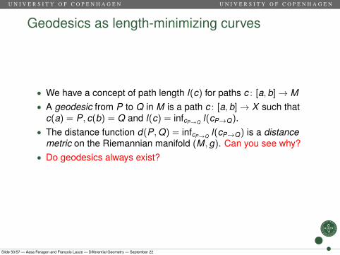
• We have a concept of path length l(c) for paths c : [a,b]→ M
• A geodesic from P to Q in M is a path c : [a,b]→ X such thatc(a) = P, c(b) = Q and l(c) = infcP→Q l(cP→Q).
• The distance function d(P,Q) = infcP→Q l(cP→Q) is a distancemetric on the Riemannian manifold (M,g).
Can you see why?
• Do geodesics always exist?
Slide 50/57 — Aasa Feragen and François Lauze — Differential Geometry — September 22
U N I V E R S I T Y O F C O P E N H A G E N U N I V E R S I T Y O F C O P E N H A G E N
Geodesics as length-minimizing curves
• We have a concept of path length l(c) for paths c : [a,b]→ M• A geodesic from P to Q in M is a path c : [a,b]→ X such that
c(a) = P, c(b) = Q and l(c) = infcP→Q l(cP→Q).
• The distance function d(P,Q) = infcP→Q l(cP→Q) is a distancemetric on the Riemannian manifold (M,g).
Can you see why?
• Do geodesics always exist?
Slide 50/57 — Aasa Feragen and François Lauze — Differential Geometry — September 22

U N I V E R S I T Y O F C O P E N H A G E N U N I V E R S I T Y O F C O P E N H A G E N
Geodesics as length-minimizing curves
• We have a concept of path length l(c) for paths c : [a,b]→ M• A geodesic from P to Q in M is a path c : [a,b]→ X such that
c(a) = P, c(b) = Q and l(c) = infcP→Q l(cP→Q).• The distance function d(P,Q) = infcP→Q l(cP→Q) is a distance
metric on the Riemannian manifold (M,g).
Can you see why?• Do geodesics always exist?
Slide 50/57 — Aasa Feragen and François Lauze — Differential Geometry — September 22

U N I V E R S I T Y O F C O P E N H A G E N U N I V E R S I T Y O F C O P E N H A G E N
Geodesics as length-minimizing curves
• We have a concept of path length l(c) for paths c : [a,b]→ M• A geodesic from P to Q in M is a path c : [a,b]→ X such that
c(a) = P, c(b) = Q and l(c) = infcP→Q l(cP→Q).• The distance function d(P,Q) = infcP→Q l(cP→Q) is a distance
metric on the Riemannian manifold (M,g). Can you see why?
• Do geodesics always exist?
Slide 50/57 — Aasa Feragen and François Lauze — Differential Geometry — September 22
U N I V E R S I T Y O F C O P E N H A G E N U N I V E R S I T Y O F C O P E N H A G E N
Geodesics as length-minimizing curves
• We have a concept of path length l(c) for paths c : [a,b]→ M• A geodesic from P to Q in M is a path c : [a,b]→ X such that
c(a) = P, c(b) = Q and l(c) = infcP→Q l(cP→Q).• The distance function d(P,Q) = infcP→Q l(cP→Q) is a distance
metric on the Riemannian manifold (M,g). Can you see why?• Do geodesics always exist?
Slide 50/57 — Aasa Feragen and François Lauze — Differential Geometry — September 22

U N I V E R S I T Y O F C O P E N H A G E N U N I V E R S I T Y O F C O P E N H A G E N
Example: Riemannian geodesics between1-dimensional Gaussian distributions• Space parametrized by (µ, σ) ∈ R× R+
• Metric 1: Euclidean inner product⇒ Euclidean geodesics
• Metric 2: Fisher information metric
• View in plane:
2
Middle figure from Costa et al, Fisher information distance: a geometrical reading
Slide 51/57 — Aasa Feragen and François Lauze — Differential Geometry — September 22

U N I V E R S I T Y O F C O P E N H A G E N U N I V E R S I T Y O F C O P E N H A G E N
Outline
1 MotivationNonlinearityRecall: Calculus in Rn
2 Differential GeometrySmooth manifoldsBuilding ManifoldsTangent SpaceVector fieldsDifferential of smooth map
3 Riemannian metricsIntroduction to Riemannian metricsRecall: Inner ProductsRiemannian metricsInvariance of the Fisher information metricA first take on the geodesic distance metricA first take on curvature
Slide 52/57 — Aasa Feragen and François Lauze — Differential Geometry — September 22
U N I V E R S I T Y O F C O P E N H A G E N U N I V E R S I T Y O F C O P E N H A G E N
A first take on curvature
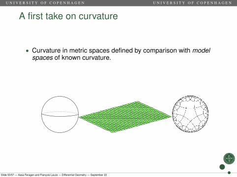
• Curvature in metric spaces defined by comparison with modelspaces of known curvature.
• Positive curvature model spaces. Spheres of curvature κ > 0:• Flat model space: Euclidean plane• Negatively curved model spaces: Hyperbolic space of curvatureκ > 0
Slide 53/57 — Aasa Feragen and François Lauze — Differential Geometry — September 22

U N I V E R S I T Y O F C O P E N H A G E N U N I V E R S I T Y O F C O P E N H A G E N
A first take on curvature
• Curvature in metric spaces defined by comparison with modelspaces of known curvature.
• Positive curvature model spaces. Spheres of curvature κ > 0:• Flat model space: Euclidean plane• Negatively curved model spaces: Hyperbolic space of curvatureκ > 0
Slide 53/57 — Aasa Feragen and François Lauze — Differential Geometry — September 22
U N I V E R S I T Y O F C O P E N H A G E N U N I V E R S I T Y O F C O P E N H A G E N
A first take on curvature
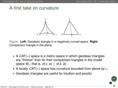
Figure : Left: Geodesic triangle in a negatively curved space. Right:Comparison triangle in the plane.
• A CAT (κ) space is a metric space in which geodesic trianglesare ”thinner” than for their comparison triangles in the modelspace Mκ; that is, d(x ,a) ≤ d(x , a).
• A locally CAT (κ) space has curvature bounded from above by κ.• Geodesic triangles are useful for intuition and proofs!
Slide 53/57 — Aasa Feragen and François Lauze — Differential Geometry — September 22

U N I V E R S I T Y O F C O P E N H A G E N U N I V E R S I T Y O F C O P E N H A G E N
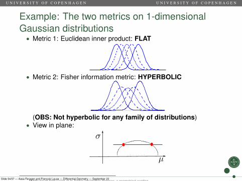
Example: The two metrics on 1-dimensionalGaussian distributions• Metric 1: Euclidean inner product: FLAT
• Metric 2: Fisher information metric: HYPERBOLIC
(OBS: Not hyperbolic for any family of distributions)• View in plane:
2
• You will see these again with Stefan!
Middle figure from Costa et al, Fisher information distance: a geometrical readingSlide 54/57 — Aasa Feragen and François Lauze — Differential Geometry — September 22
U N I V E R S I T Y O F C O P E N H A G E N U N I V E R S I T Y O F C O P E N H A G E N
Example: The two metrics on 1-dimensionalGaussian distributions• Metric 1: Euclidean inner product: FLAT
• Metric 2: Fisher information metric: HYPERBOLIC
(OBS: Not hyperbolic for any family of distributions)• View in plane:
2
• You will see these again with Stefan!
Middle figure from Costa et al, Fisher information distance: a geometrical readingSlide 54/57 — Aasa Feragen and François Lauze — Differential Geometry — September 22

U N I V E R S I T Y O F C O P E N H A G E N U N I V E R S I T Y O F C O P E N H A G E N
Example: The two metrics on 1-dimensionalGaussian distributions• Metric 1: Euclidean inner product: FLAT
• Metric 2: Fisher information metric: HYPERBOLIC
(OBS: Not hyperbolic for any family of distributions)• View in plane:
2
• You will see these again with Stefan!Middle figure from Costa et al, Fisher information distance: a geometrical reading
Slide 54/57 — Aasa Feragen and François Lauze — Differential Geometry — September 22
U N I V E R S I T Y O F C O P E N H A G E N U N I V E R S I T Y O F C O P E N H A G E N
Relation to sectional curvature
• CAT (κ) is a weak notion of curvature• Stronger notion of sectional curvature (requires a little more
Riemannian geometry)
TheoremA smooth Riemannian manifold M is (locally) CAT (κ) if and only if thesectional curvature of M is ≤ κ.
Slide 55/57 — Aasa Feragen and François Lauze — Differential Geometry — September 22

U N I V E R S I T Y O F C O P E N H A G E N U N I V E R S I T Y O F C O P E N H A G E N
Example of insight with CAT (κ):MDS and manifold learning lie to you• Given a distance matrix Dij = d(xi , xj ) for a dataset
X = {x1, . . . , xn} residing on a manifold M, where d is ageodesic metric.
• Assume that Z = {z1, . . . , zn} ⊂ Rd is an embedding of Xobtained through MDS or manifold learning.
• Common belief: If d large, then Z is a good (perfect?)representation of X .
Slide 56/57 — Aasa Feragen and François Lauze — Differential Geometry — September 22

U N I V E R S I T Y O F C O P E N H A G E N U N I V E R S I T Y O F C O P E N H A G E N
Example of insight with CAT (κ):MDS and manifold learning lie to you
• Truth: If there exists a map f : M → Rd such that‖f (a)− f (b)‖ = d(a,b) for all a,b ∈ M, then
• f maps geodesics to straight lines• M is CAT (0)• M is not CAT (κ) for any κ < 0• ⇒ M is flat
• That is, if M is not flat, MDS and manifold learning lie to you• (but sometimes lies are useful)
Slide 56/57 — Aasa Feragen and François Lauze — Differential Geometry — September 22

U N I V E R S I T Y O F C O P E N H A G E N U N I V E R S I T Y O F C O P E N H A G E N
Example of insight with CAT (κ):MDS and manifold learning lie to you
• Truth: If there exists a map f : M → Rd such that‖f (a)− f (b)‖ = d(a,b) for all a,b ∈ M, then
• f maps geodesics to straight lines• M is CAT (0)• M is not CAT (κ) for any κ < 0
• ⇒ M is flat• That is, if M is not flat, MDS and manifold learning lie to you• (but sometimes lies are useful)
Slide 56/57 — Aasa Feragen and François Lauze — Differential Geometry — September 22
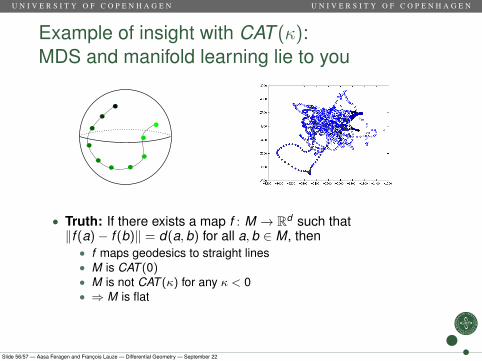
U N I V E R S I T Y O F C O P E N H A G E N U N I V E R S I T Y O F C O P E N H A G E N
Example of insight with CAT (κ):MDS and manifold learning lie to you
• Truth: If there exists a map f : M → Rd such that‖f (a)− f (b)‖ = d(a,b) for all a,b ∈ M, then
• f maps geodesics to straight lines• M is CAT (0)• M is not CAT (κ) for any κ < 0• ⇒ M is flat
• That is, if M is not flat, MDS and manifold learning lie to you• (but sometimes lies are useful)
Slide 56/57 — Aasa Feragen and François Lauze — Differential Geometry — September 22

U N I V E R S I T Y O F C O P E N H A G E N U N I V E R S I T Y O F C O P E N H A G E N
Example of insight with CAT (κ):MDS and manifold learning lie to you
• Truth: If there exists a map f : M → Rd such that‖f (a)− f (b)‖ = d(a,b) for all a,b ∈ M, then
• f maps geodesics to straight lines• M is CAT (0)• M is not CAT (κ) for any κ < 0• ⇒ M is flat
• That is, if M is not flat, MDS and manifold learning lie to you
• (but sometimes lies are useful)
Slide 56/57 — Aasa Feragen and François Lauze — Differential Geometry — September 22
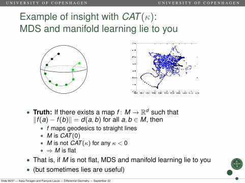
U N I V E R S I T Y O F C O P E N H A G E N U N I V E R S I T Y O F C O P E N H A G E N
Example of insight with CAT (κ):MDS and manifold learning lie to you
• Truth: If there exists a map f : M → Rd such that‖f (a)− f (b)‖ = d(a,b) for all a,b ∈ M, then
• f maps geodesics to straight lines• M is CAT (0)• M is not CAT (κ) for any κ < 0• ⇒ M is flat
• That is, if M is not flat, MDS and manifold learning lie to you• (but sometimes lies are useful)
Slide 56/57 — Aasa Feragen and François Lauze — Differential Geometry — September 22

U N I V E R S I T Y O F C O P E N H A G E N U N I V E R S I T Y O F C O P E N H A G E N
A message from Stefan for tomorrow’s practical
Check out course webpage for installation instructions!http://image.diku.dk/MLLab/IG4.php
Slide 57/57 — Aasa Feragen and François Lauze — Differential Geometry — September 22