Tyler P. Jones and Tom Thorvaldsen - FFI · Tyler P. Jones and Tom Thorvaldsen Norwegian Defence...

Experiences from ultrasound testing – Olympus Omniscan MX and DolphiCam CF08/CF16

FFI-rapport 2015/00589

Tyler P. Jones and Tom Thorvaldsen

ForsvaretsforskningsinstituttFFI

N o r w e g i a n D e f e n c e R e s e a r c h E s t a b l i s h m e n t


Experiences from ultrasound testing – Olympus Omniscan MX and DolphiCam CF08/CF16

Tyler P. Jones and Tom Thorvaldsen

Norwegian Defence Research Establishment (FFI)

8 January 2016

2 FFI-rapport 2015/00589


136901

P: ISBN 978-82-464-2634-1 E: ISBN 978-82-464-2635-8

Keywords

Ikke-destruktiv inspeksjon

Ultralyd

Materiallære

Materialteknologi

Vedlikehold

Approved by

Rune Lausund Forskningsleder

Jon E. Skjervold Avdelingssjef

FFI-rapport 2015/00589 3

English summary Modern military platforms, such as the NH90 helicopter and the F-35 Joint Strike Fighter, consist of a large percentage of light-weight materials, such as composites. New materials require new and different techniques for efficient and reliable inspection to detect damages that may be critical for the performance and safety of the platform. This is particularly relevant for helicopters/aircrafts, but also for land vehicles and ships. Non-destructive inspection methods are defined and employed as part of the maintenance system for modern composite structures, but more research and testing is required. FFI supports the Norwegian Armed forces and the Norwegian Defence Logistics Organization (NDLO) in this work. This study was performed to compare and contrast two different types of ultrasonic non-destructive inspection (NDI) systems, while investigating simulated damages in carbon fibre reinforced polymer (CFRP) panels and repairs in a sandwich panel. The ultrasound systems investigated in this study were the Olympus Omniscan MX, a common phased-array unit, and two models of the DolphiTech DolphiCam™, which is a relatively new matrix-array system for area scan. Four CFRP panels were produced with simulated delaminations consisting of Teflon® and aluminium inclusions, blind drill holes, and impact damages. A glass fibre/Nomex honeycomb sandwich panel with scarf repairs was also investigated. In total, there were over 70 different types and depths of damage investigated by the NDI systems. Ultrasound imagery of the simulated damages provided information on the accuracy, applicability, and relative strengths and weaknesses of the two systems. The DolphiTech cameras, consisting of two models designed for 8 mm and 16 mm thick CFRP structures, DolphiCam™ CF08 and DolphiCam™ CF16, respectively, provided very detailed imagery and depth measurements of all types of simulated damages. Defect features of less than 1.0 mm out of plane could easily be detected and measured. Further, the DolpiTech cameras required minimal set-up time, and performed well in both freezing and controlled room temperature environments. The Olympus Omniscan MX system, requiring a longer set-up time and having larger support equipment requirements, was also able to detect the simulated damage areas. Finally, the Olympus Omniscan MX system performed quicker inspections of much larger areas compared to the DolphiTech cameras. This study found that the two types of NDI systems offered complementary strengths and weaknesses when employed for detection of simulated damages in CFRP materials. Also, DolphiCam™ CF08 showed surprisingly good results at investigating bonded scarf repairs to the glass fibre/Nomex sandwich panel.


Sammendrag Moderne militære plattformer, som blant annet NH90 og F-35, består av en stor andel lettvektsmaterialer, slik som kompositter. Bruk av nye materialer krever andre teknikker for å kunne gjøre en effektiv inspeksjon, for på den måten å avdekke skader som kan være kritisk for yteevnen og sikkerheten til plattformen. Dette er spesielt viktig for helikoptre/fly, men er også relevant for landgående fartøy og skip. Ikke-destruktive inspeksjonsmetoder er definert og benyttet som del av vedlikeholdssystemet for moderne komposittkonstruksjoner, men mer forskning og testing er nødvendig. FFI støtter Forsvaret og FLO i dette arbeidet. Denne studien er utført for å sammenlikne to ulike ultralydsystemer for ikke-destruktiv inspeksjon, ved å se på simulerte skader i karbonfiberpaneler og et reparert sandwich-panel. Ultralydsystemene som ble sett på i denne studien, var Olympus Omniscan MX, med en tradisjonell “phased-array”-enhet, og to modeller av DolphiCam™ fra DolphiTech, som har et relativt nytt matrisesystem for flateskann. Fire karbonfiberpaneler ble produsert, med simulerte delamineringer i form av Teflon®- og aluminiumsinklusjoner, med borede hull og med slagskader. Et reparert sandwich-panel med hudlag i glassfiberkompositt og kjernemateriale av Nomex (“honeycomb”) ble også studert. Totalt ble mer enn 70 forskjellige typer skader og dybder undersøkt med inspeksjonsutstyret. Ultralydbildene av de simulerte skadene ga informasjon om nøyaktighet, anvendbarhet og relative styrker og svakheter ved de to systemene. Kameraene fra DolphiTech, som besto av to modeller som er designet for karbonfiberpaneler med en tykkelse på 8 mm og 16 mm, henholdsvis DolphiCam™ CF08 og DolphiCam™ CF16, ga detaljerte bilder og dybdeinformasjon for alle typer simulerte skader. Defekter med en utstrekning på mindre enn 1,0 mm i tykkelsesretningen ble lett oppdaget og målt. Videre krevde DolphiTech-kameraene minimalt med tid til å sette opp systemet, og fungerte bra både i kalde omgivelser og ved romtemperatur. Olympus Omniscan MX krevde mer tid til å sette opp systemet og har flere komponenter som del av oppsettet. Dette systemet var også i stand til å detektere alle skadene, og var i stand til å inspisere et større areal hurtigere sammenliknet med DolphiTech-kameraene. Denne studien har vist at de to systemene for ikke-destruktiv inspeksjon har komplementære styrker og svakheter for deteksjon av simulerte skader i karbonfiberpaneler. DolphiCam™ CF08 ga for øvrig overraskende gode resultatet ved inspeksjon av det reparerte glassfiber/Nomex sandwich-panelet.


Contents

1 Introduction 7

2 Equipment from DolphiTech 7

3 Equipment from Olympus 8

4 Test panels 9 4.1 CFRP panel with flat bottomed drilled holes 10 4.2 CFRP panel with inclusions 10 4.3 CFRP panel with impact damages 12 4.4 Glass fibre/Nomex sandwich panel 13

5 Test case 1: Monolithic CFRP panel with flat bottomed drilled holes 13

5.1 DolphiCam™ CF08 14 5.2 DolphiCam™ CF16 16 5.3 Omniscan MX 18

6 Test case 2: Monolithic CFRP panel with inclusions 19 6.1 DolphiCam™ CF08 19 6.1.1 Rectangular aluminium inclusions 19 6.1.2 Circular aluminium inclusions 20 6.1.3 Rectangular one layer Teflon® tape inclusions 21 6.1.4 Rectangular two layer Teflon® tape inclusions 22 6.1.5 Circular one layer Teflon® tape inclusions 24 6.1.6 Circular two layer Teflon® tape inclusions 25 6.2 DolphiCam™ 16mm 26 6.2.1 Rectangular aluminium inclusions 26 6.2.2 Circular aluminium inclusions 27 6.2.3 Rectangular one layer Teflon® tape inclusions 28 6.2.4 Rectangular two layer Teflon® tape inclusions 29 6.2.5 Circular one layer Teflon® tape inclusions 31 6.2.6 Circular two layer Teflon® tape inclusions 32 6.3 Omniscan MX 33 6.3.1 Rectangular aluminium inclusions 33 6.3.2 Circular aluminium inclusions 34 6.3.3 Rectangular one layer Teflon® tape inclusions 35 6.3.4 Rectangular two layer Teflon® tape inclusions 36


6.3.5 Circular one layer Teflon® tape inclusions 37 6.3.6 Circular two layer Teflon® tape inclusions 38

7 Test case 3: Impact damaged panel 39 7.1 DolphiCam™ CF08 39 7.2 DolphiCam™ CF16 40 7.3 Omniscan MX 41

8 Test case 4: Glass fibre/Nomex sandwich panel 43

9 Discussion and conclusion 45

Acknowledgements 48

Appendix A User’s Guide to Olympus Onmiscan MX 49 A.1 Introduction 49 A.2 Basic Set-up 49 A.3 Calibrating Material Speed of Sound 51 A.4 C-scan with VersaMOUSE 53 A.5 Creating a Report 54 A.6 File transfer to USB 55

References 56


1 Introduction This report describes the new experiences from non-destructive inspection (NDI) using ultrasound. This study is a continuation of the work done in the FFI project 379901 [1;2] and the results presented at the NATO STO AVT-224 workshop [3]. Ultrasound is considered as one relevant method for non-destructive testing and inspection of military platforms and equipment, as part of the maintenance and structural health monitoring (SHM) system. Different requirements are set for the inspection procedures in a workshop environment and at a forward operating base. The inspection equipment applied may also be different due to this. In this report, two different ultrasound systems, including three instruments, for non-destructive inspection are tested and compared: 1) Olympus Omniscan MX, 2) DolphiCam™ CF08 and 3) DolphiCam™ CF16. The main objective of the current report is to quantify the detection range and overall performance of the instruments. The inspection is performed on a set of composite panels with simulated (and known) defects, which are representative for defects in military equipment and applications.

2 Equipment from DolphiTech DolphiTech AS has developed two different ultrasound instruments for non-destructive inspection of carbon fibre reinforced polymer (CFRP) composites, see Figure 2.1. DolphiCam™ CF08 is designed for detecting defects in the depth range from 0 to 8 mm, whereas DolphiCam™ CF16 is designed for detecting defects in the range from 0 to 16 mm.

Figure 2.1: DolphiCam™ CF08 (in back) and DolphiCam™ CF16 (in front) from DolphiTech.


FFI bought a prototype version of DolphiCam™ CF08 in 2012. As part of the deal and collaboration between DolphiTech and FFI, the latest version of DolphiCam™ CF08 has been provided. The DolphiCam™ CF08 (compared to the instrument tested and reported in [1]) has an improved dry coupling transducer pad. The new pad is made of a material that allows a more rough use, and makes it easier to do inspections also on rougher surfaces without applying a contact medium (such as gel or water). According to DolphiTech, the optional use of water or contact gel might reduce the ultrasound noise and provide better images in some cases. It is also commented that this will reduce the forces needed to get good mechanical contact between the dry coupling and the material, improving the usability of the system. Besides the new dry coupling pad, the camera specifications are unchanged. The DolphiCam™ CF16 has been made available for FFI (free of charge) for some weeks, for testing. The CF16 model has a bit thicker coupling transducer pad and is a bit larger. Except that, this instrument is very similar to DolphiCam™ CF08, and is operated in the same way by the inspector. A more detailed description about the use, new software tools, as well as the technical details of the instruments, is available on DolphiTech’s home pages [4].

3 Equipment from Olympus Olympus has developed instruments for non-destructive inspection of different materials. The Olympus Omniscan MX, see Figure 3.1, is applied for ultrasound inspection. The software contains a database for various materials, which includes, among others, the sound speed for the material. Since composites have varying properties due to the materials used, the material properties need in this case to be set by the operator. This is also the case for the geometric parameters of the object of investigation. A quick user’s guide is included in Vedlegg A. Different probes are available, depending on the type of material and inspection to be performed. In the current study, a standard phased-array probe 5 Mz linear array (5.0L64-NW1) has been used, see Figure 3.2 . To avoid near-field problems, a wedge is included in the set-up (SNW1-0L-AQ25). The VersaMOUSE is applied for position monitoring.


Figure 3.1: Olympus Omniscan MX. Set-up at FFI.

Figure 3.2: The probe and wedge for the ultrasound scan. The VersaMOUSE is used for position monitoring.

4 Test panels Different composite panels with known defects have been produced and tested in this study. This includes a monolithic CFRP panel with holes, where the holes are drilled into the composite at different depths, and a second monolithic CFRP panel with aluminium and Teflon® tape inclusions that mimic delaminations in the composite. The third and fourth test panels are monolithic CFRP panels that were impacted in a controlled way at different energy levels. All four panels were produced after FFI’s specifications by High Performance Composites [5]. After production, the third and fourth panels were impact tested using an air pressured impactor (not a drop test). In addition, a sandwich composite with a Nomex honeycomb core and glass fibre reinforced polymer (GFRP) skins was inspected; one of the skins had been repaired employing the scarf repair technique.


4.1 CFRP panel with flat bottomed drilled holes

The monolithic panel with flat bottomed drilled holes are shown in Figure 4.1. The panel is made of the prepreg HexPly® 6376-HTA(12k)5.5-29.5% [6], which has the form of unidirectional mats delivered by Hexcel. The lay-up of the plate is 75 layers of the unidirectional mats, placed in [0/90] pattern, giving a total thickness of around 10 mm. The panel was produced in an autoclave with a pressure of 0.7 MPa (= 7 bar), and cured according to the procedure provided by the material supplier. After curing, flat holes with a diameter of 10 mm were drilled at different depths.

Figure 4.1: Test panel with drilled holes.

4.2 CFRP panel with inclusions

The CFRP panel with inclusions is produced by the same materials and techniques as described in Section 4.1. However, in this case flat rectangular and circular sheets of aluminium, as well as two thicknesses of Teflon® tape, were included between the prepreg fabric layers, at different depths. The total thickness of the panel is around 10 mm. The panel is shown in Figure 4.2, and a sketch of the positioning of the different inclusions is shown in Figure 4.3. Note that the sketch in Figure 4.3 points out the position and type of inclusions from the rough side of the panel, whereas the picture in Figure 4.2 is displays the smooth side, i.e. the opposite side.


Figure 4.2: Test panel with inclusions.


Figure 4.3: Sketch of the inclusions in the test panel. The inclusions are centred at the given position for each inclusion. Note that this sketch is showing the opposite side of the panel, compared to the picture in Figure 4.2.

4.3 CFRP panel with impact damages

Two additional CFRP panels, with thickness 3 mm and 5 mm, were produced by the same materials and techniques as described in Section 4.1. These panels were impacted at different energy levels, see Figure 4.4.

Depth in mm:

1,5

0,5 1,0

3,0

2,0

2,5

4,5

3,5 4,0

5,0

Size of defect (mm) 20 0 mm x 10 0 mm

Diameter = 10 0 mm

Teflon

t = x

Teflon

t = x

Al-folie

Teflon

Teflon

Al-folie

25 25 50 50 50 50

50

25 50

50

50

50

50

50

50

50 25

50 50 50 50 50


(a) (b)

Figure 4.4: CFRP panels with impacted damages. a) Panel with thickness of 3 mm; b) panel with thickness of 5 mm.

4.4 Glass fibre/Nomex sandwich panel

A glass fibre/Nomex sandwich test panel was obtained from FLO Luftkapasiteter/AIM Norway. The panel had a 12.2 mm core made of honeycomb, with 1.0 mm GFRP skins on each side. The skin (on one side) was repaired according to a scarf repair procedure, at two locations. No details are available for the applied materials or the exact repair procedure.

Figure 4.5: Sandwich panel with Nomex honeycomb core and glass fibre reinforced polymer

skins.

5 Test case 1: Monolithic CFRP panel with flat bottomed drilled holes

In this first test case, we consider the CFRP panel with flat bottomed drilled holes, as described in Section 4.1. The panel was inspected from the opposite side from where the holes were drilled, which means that there is composite material between the transducer and the bottom of the holes.


The holes are thus “blind” to the ultrasound transducer. A sketch of the set-up is shown in Figure 5.1.

5.1 DolphiCam™ CF08

With the previous prototype version of the DolphiCam™ CF08, as reported in [1], the defects in the panel were detected in the composite thickness range from 1 mm to 6 mm. Defects that were positioned deeper in the material were not detected. Two example images are shown in Figure 5.2 and Figure 5.3 for the defects with a composite thickness of 1 mm and 6 mm, respectively.

Figure 5.2: Image from applying a prototype version of the DolphiCam™ CF08 for the CFRP panel with flat bottomed drilled holes. The composite thickness is 1 mm.

Ultrasound scanner unit

Composite thickness Hole depth

Figure 5.1: A sketch of the scanning of the panel with blind holes. The scanner is placed on the opposite side of the hole opening. The holes have different depths.


Figure 5.3: Image from applying a prototype version of the DolphiCam™ CF08 for the CFRP panel with flat bottomed drilled holes. The composite thickness is 6 mm.

The same case as shown in Figure 5.2, now using the latest version of the DolphiCam™ CF08, is shown in Figure 5.4. Comparing the two versions of the DolphiCam™ CF08 camera, the image resolution (driven by the number and type of transducers) is nearly identical. However, the updated image processing software makes screen defect detection much easier for the operator. Furthermore, it was found that adjusting the time of flight (TOF) signal contrast, with a higher weighting around the depth of interest, provided an increased ability to detect simulated defects at the extreme minimums and maximums of the camera inspection depth range. The image from the inspection of the drilled hole at a depth of 8 mm is shown in Figure 5.5, demonstrating the ability of the CF08 camera to detect defects at its maximum range. With increasing composite thickness, the details of the hole defects are decreased. However, detectability could be maintained at a consistent high level by applying a time corrected gain to the amplitude signals.


Figure 5.4: Image of the blind hole with composite thickness of 1 mm, using the new DolphiCam™ CF08.

Figure 5.5: Image of blind hole with composite thickness of 8 mm, using the new DolphiCam™ CF08.


The DolphiCam™ CF16 camera is functionally the same as the CF08 version, with only minor changes made to the hardware and software to optimize the images for thicker composites, i.e. up to a thickness of 16 mm. The most significant hardware difference between the CF08 and the


CF16 camera is the thicker dry coupling pad, which is giving the transducer matrix a larger stand-off distance from the composite surface. The higher amplitude of the transmitted pulses for the CF16 camera can be seen in Figure 5.6, where the signal reflections from the near-field surface of the blind hole face have large amplitudes. DolphiCam™ CF16 performs qualitatively the same as DolphiCam™ CF08 for simulated near-field defects. In this case, the TOF signal contrast for the near-field defect was not weighted.

Figure 5.6: Image of a blind hole with composite thickness of 1 mm, using the DolphiCam™ CF16 camera. The deepest simulated and detected defect, consisting of a 1 mm deep blind hole with a composite thickness of 9 mm, is given in Figure 5.7. In this case, the TOF scale was adjusted for higher contrast, due to the small distance (i.e. 1 mm) between the blind hole face depth and the back surface of the composite. The TOF signals have a higher contrast weighting applied around the depth of interest to better distinguish the characteristics of the flat bottomed blind hole. Increasing composite thickness led to a decrease in the detail imagery of the defects. However, detectability could be maintained at a consistent high level by applying a time corrected gain to the amplitude signals for the DolphiCam™ CF16 camera.


Figure 5.7: Image of a blind hole with composite thickness of 9 mm, using the DolphiCam™ CF16 camera.

5.3 Omniscan MX

The Omniscan MX instrument from Olympus, see Section 3, was also used to inspect the various depths of boreholes in the CFRP panel. A representative result from the flat bottomed blind hole inspections by the Omniscan MX is given in Figure 5.8, in this case for the hole with a composite thickness of 7 mm. The signal from the face surface of the blind hole can be seen in the A-scan as a signal return with approximately 60 per cent amplitude of the transmitted pulse. Furthermore, the high degree of flexibility in the Omniscan MX system allowed for all depths of holes to be imaged with the same degree of detectability and clarity.


Figure 5.8: Image of the blind hole with a composite thickness of 7 mm, using the Omniscan MX instrument.

6 Test case 2: Monolithic CFRP panel with inclusions In this next test case, the CFRP panel with different inclusions is investigated, see Section 4.2. The results for three types of defects (aluminium and two thicknesses of Teflon® tape), with different geometry (circular and rectangular), are reported for each instrument.


6.1.1 Rectangular aluminium inclusions

DolphiCam™ CF08 was used to inspect the laminated rectangular aluminium inclusions with increasing depth of inclusion from 0.5 mm to 5 mm. Results for the minimum and maximum depth of rectangular aluminium inclusion are given in Figure 6.1 and Figure 6.2, respectively.


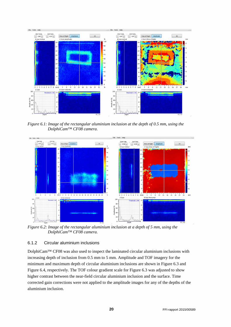
Figure 6.1: Image of the rectangular aluminium inclusion at the depth of 0.5 mm, using the DolphiCam™ CF08 camera.

Figure 6.2: Image of the rectangular aluminium inclusion at a depth of 5 mm, using the DolphiCam™ CF08 camera.

6.1.2 Circular aluminium inclusions

DolphiCam™ CF08 was also used to inspect the laminated circular aluminium inclusions with increasing depth of inclusion from 0.5 mm to 5 mm. Amplitude and TOF imagery for the minimum and maximum depth of circular aluminium inclusions are shown in Figure 6.3 and Figure 6.4, respectively. The TOF colour gradient scale for Figure 6.3 was adjusted to show higher contrast between the near-field circular aluminium inclusion and the surface. Time corrected gain corrections were not applied to the amplitude images for any of the depths of the aluminium inclusion.


Figure 6.3: Image of the circular aluminium inclusion at a depth of 0.5 mm, using the DolphiCam™ CF08 camera.

Figure 6.4: Image of the circular aluminium inclusion at a depth of 5 mm, using the DolphiCam™ CF08 camera.

6.1.3 Rectangular one layer Teflon® tape inclusions

The images when using the DolphiCam™ CF08 camera for the case of rectangular single layer Teflon® inclusions at depths of 0.5 mm and 5 mm are displayed in Figure 6.5 and Figure 6.6, respectively. The TOF colour gradient scales for both (displayed) depths were adjusted to provide clearer discrimination of features. It can also be seen that there exist signal reflections from the inclusion that could lead to inaccurate near-field depth measurement.


The 5 mm deep single layer Teflon® inclusion exhibits a feature that is visible in both the amplitude and TOF imagery.

Figure 6.5: Image of rectangular single layer Teflon® inclusion at a depth of 0.5 mm, using the DolphiCam™ CF08 camera.

Figure 6.6: Image of rectangular single layer Teflon® inclusion at a depth of 5 mm, using the DolphiCam™ CF08 camera.

6.1.4 Rectangular two layer Teflon® tape inclusions

The images when using the DolphiCam™ CF08 camera for the case of rectangular double layer Teflon® inclusions at depths of 0.5 mm and 5 mm are displayed in Figure 6.7 and Figure 6.8, respectively. The TOF colour gradient scales for both (displayed) depths of double layer Teflon® inclusions were adjusted to provide clearer discrimination of features. It can also be seen that there exist signal reflections from the inclusion that could lead to inaccurate near-field depth


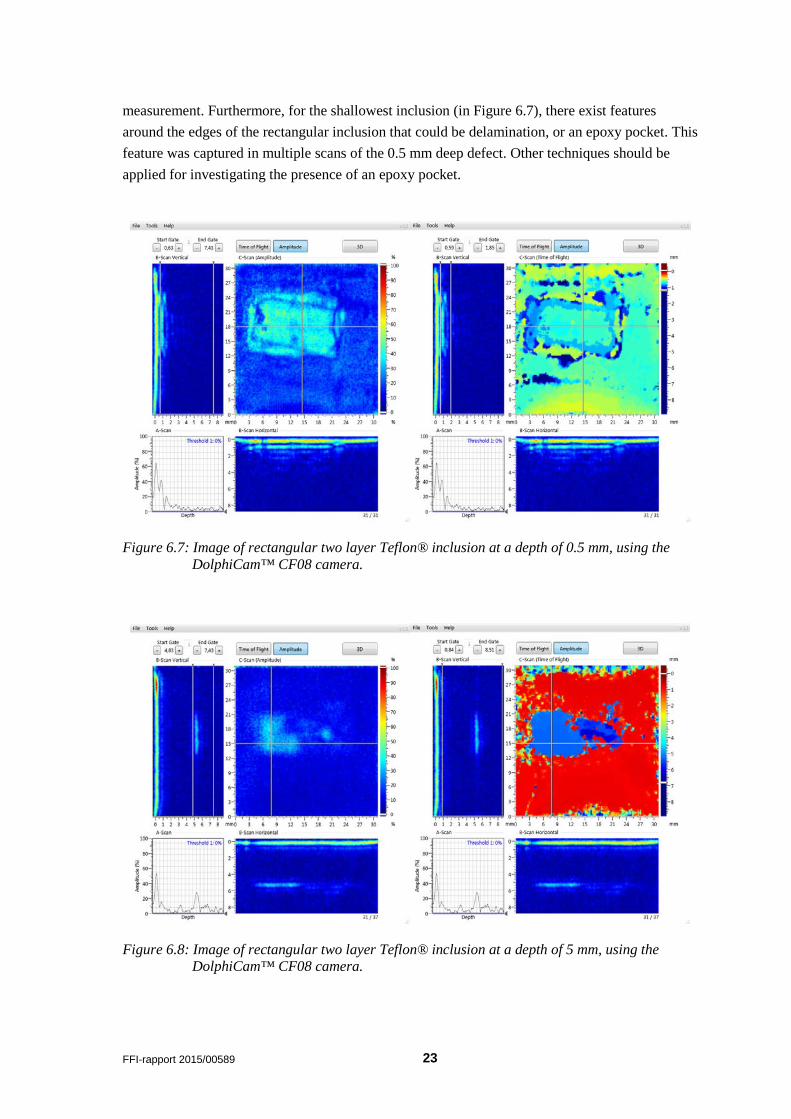
measurement. Furthermore, for the shallowest inclusion (in Figure 6.7), there exist features around the edges of the rectangular inclusion that could be delamination, or an epoxy pocket. This feature was captured in multiple scans of the 0.5 mm deep defect. Other techniques should be applied for investigating the presence of an epoxy pocket.

Figure 6.7: Image of rectangular two layer Teflon® inclusion at a depth of 0.5 mm, using the DolphiCam™ CF08 camera.

Figure 6.8: Image of rectangular two layer Teflon® inclusion at a depth of 5 mm, using the DolphiCam™ CF08 camera.


6.1.5 Circular one layer Teflon® tape inclusions

The images when using the DolphiCam™ CF08 camera for the case of circular single layer Teflon® inclusions at depths of 0.5 mm and 5 mm are displayed in Figure 6.9 and Figure 6.10, respectively. The TOF colour gradient scales for both depths of single layer Teflon® inclusions were adjusted to provide clearer discrimination of features. It can also be seen that there exist signal reflections from the near-field inclusion in Figure 6.9, which gives a false double at the depth of 1 mm. The imagery of the 5 mm deep single layer Teflon® inclusion displayed an apparent out of plane, or wavy, feature. This waviness from 0.5 to 1.0 mm was measured in multiple scans of the inclusion, and determined not to be a signal artefact. The feature can be observed in the lower centre of the inclusions in Figure 6.10.

Figure 6.9: Image of circular single layer Teflon® inclusion at a depth of 0.5 mm, using the DolphiCam™ CF08 camera.


Figure 6.10: Image of circular single layer Teflon® inclusion at a depth of 5 mm, using the DolphiCam™ CF08 camera.

6.1.6 Circular two layer Teflon® tape inclusions

Results from DolphiCam™ CF08 inspection of circular two layer Teflon® inclusions are presented at depths of 0.5 mm and 5 mm in Figure 6.11 and Figure 6.12, respectively. For the near-field TOF imagery it was necessary to adjust the colour gradient scaling to produce the image for the defect at a depth of 0.5 mm; there exist near-field signal reflections leading to a false reading at a depth of 1 mm deep for the 0.5 mm deep inclusion. TOF colour gradient scaling is unaltered in Figure 6.12. Further, it is observed in this latter case that the 5 mm deep two layer Teflon® inclusion displays an out of plane wrinkle feature. Other non-destructive test methods should be applied to investigate this further.


Figure 6.11: Image of a circular two layer Teflon® inclusion at a depth of 0.5 mm, using the DolphiCam™ CF08 camera.

Figure 6.12: Image of a circular two layer Teflon® inclusion at a depth of 5 mm, using the DolphiCam™ CF08 camera.

6.2 DolphiCam™ 16mm


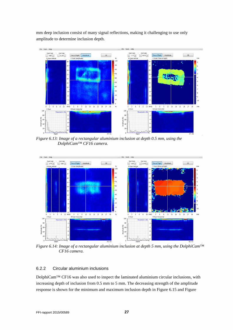
Results from the DolphiCam™ CF16 inspection of the rectangular aluminium inclusions are presented in Figure 6.13 and Figure 6.14 for the inclusion depth of 0.5 mm and 5 mm, respectively. At both near-field and far-field the TOF colour gradient scaling was adjusted to provide better discrimination of inclusion features and depth. The near-field signals for the 0.5


mm deep inclusion consist of many signal reflections, making it challenging to use only amplitude to determine inclusion depth.

Figure 6.13: Image of a rectangular aluminium inclusion at depth 0.5 mm, using the DolphiCam™ CF16 camera.

Figure 6.14: Image of a rectangular aluminium inclusion at depth 5 mm, using the DolphiCam™ CF16 camera.


DolphiCam™ CF16 was also used to inspect the laminated aluminium circular inclusions, with increasing depth of inclusion from 0.5 mm to 5 mm. The decreasing strength of the amplitude response is shown for the minimum and maximum inclusion depth in Figure 6.15 and Figure


6.16, respectively. The TOF colour gradient scaling was not adjusted from the standard full spectrum setting for all depths of inclusions.

Figure 6.15: Image of a circular aluminium inclusion at depth 0.5 mm, using the DolphiCam™ CF16 camera.

Figure 6.16: Image of a circular aluminium inclusion at depth 5 mm, using the DolphiCam™ CF16 camera.


The results from DolphiCam™ CF16 inspection of the rectangular single layer Teflon® inclusions at depths of 0.5 mm and 5 mm are shown in Figure 6.17 and Figure 6.18, respectively. The TOF colour gradient scale for all depths of this inclusion type was not from the standard full spectrum setting. It should also be noted that, in this case, there exist signal reflections from the inclusion, which could lead to inaccurate near-field depth measurement for the 0.5 mm inclusion.


Figure 6.17: Image of a rectangular single layer Teflon® inclusion at a depth of 0.5 mm, using the DolphiCam™ CF16 camera.

Figure 6.18: Image of a rectangular single layer Teflon® inclusion at a depth of 5 mm, using the DolphiCam™ CF16 camera.


The results for the DolphiCam™ CF16 inspections of the rectangular two layer Teflon® inclusions at depths of 0.5 mm, 1 mm and 5 mm are displayed in Figure 6.19, Figure 6.20, and Figure 6.21, respectively. For both near-field scans, i.e. the inclusion at depths 0.5 mm and 1.0 mm, the TOF colour gradient scaling was adjusted to provide better image quality. As shown in Figure 6.19, there exist features around the edges of the rectangular inclusion that could be a delamination or an epoxy pocket. This feature was captured in multiple scans of the 0.5 mm deep defect. Other inspection techniques may be required for further analysis.


Figure 6.19: Image of a rectangular two layer Teflon® inclusion at a depth of 0.5mm, using the DolphiCam™ CF16 camera.

Figure 6.20: Image of a rectangular two layer Teflon® inclusion at a depth of 1 mm, using the DolphiCam™ CF16 camera.


Figure 6.21: Image of a rectangular two layer Teflon® inclusion at a depth of 5mm, using the DolphiCam™ CF16 camera.


The results for the DolphiCam™ CF16 inspections of the circular one layer Teflon inclusions at depths 0.5 mm and 5.0 mm are displayed in Figure 6.22 and Figure 6.23, respectively. The TOF color gradient scaling was adjusted for the two inclusion depths presented here. Visible in Figure 6.24, both for the amplitude and the TOF images, is an apparent feature that exists out of plane with the majority of the tape inclusion. The vertical B-scan imagery shows this non-uniformity. Moreover, the TOF picture indicates a depth variation for the current inclusion of approximately 0.5-1.0 mm. Finally, the near field inclusion displays multiple signal reflections and a degree of false doubling of the amplitude signals.

Figure 6.22: Image of a circular single layer Teflon® inclusion at a depth of 0.5mm, using the

DolphiCam™ CF16 camera.


Figure 6.23: Image of a circular single layer Teflon® inclusion at a depth of 5.0mm, using the DolphiCam™ CF16 camera.


The results for DolphiCam™ CF16 inspection of the circular two layer Teflon® inclusions at depths 0.5 mm and 5.0 mm is shown in Figure 6.23 and Figure 6.24. The TOF color gradient scaling was adjusted only for the inclusion at depth 0.5mm. The near field inclusion displays multiple signal reflections and a degree of false doubling of the amplitude signals. Furthermore, as observed in Figure 6.26, the inclusion at depth 5.0mm displays an out of plane wrinkle feature.

Figure 6.24: Image of a circular two layer Teflon® inclusion at a depth of 0.5mm, using the DolphiCam™ CF16 camera.


Figure 6.25: Image of a circular two layer Teflon® inclusion at a depth of 5mm, using the DolphiCam™ CF16 camera.

6.3 Omniscan


The results of an Olympus Omniscan MX linear encoded scan of the rectangular aluminum inclusions are displayed in Figure 6.26. The images indicate the detected depth and areal size of the inclusions. Variations in the displayed signal strength of the B-scan for the simulated defects are due to the profile line intersection, as displayed in the C-scan. Significant signal reflections are observed for both near field and far field defect returns. All rectangular aluminum inclusions were easily detected with the scan area of 420mm x 64mm, completed in less than one minute.


Figure 6.26: Image of the rectangular aluminium inclusions, using Omniscan MX.


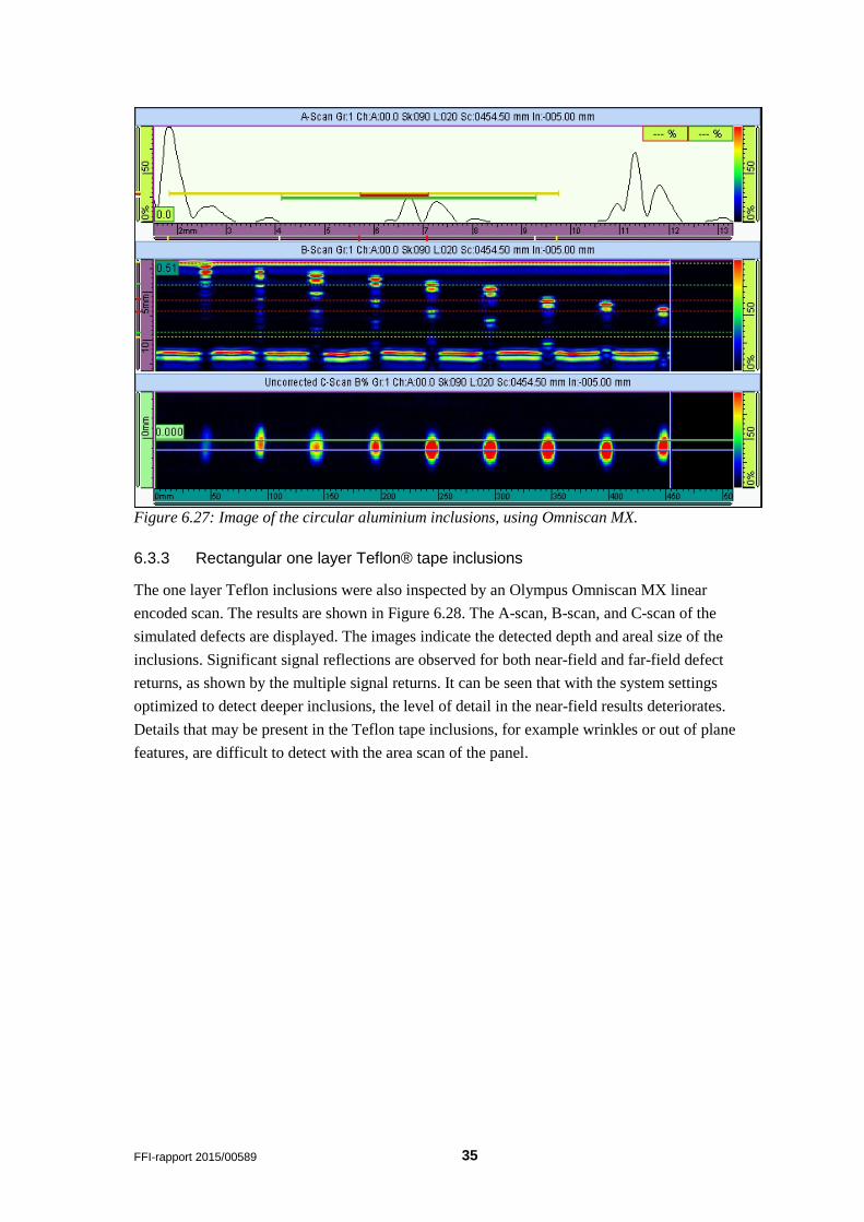
The results of an Olympus Omniscan MX linear encoded scan of the circular aluminium inclusions are presented in Figure 6.27. The A-scan, B-scan, and C-scan of the simulated defects are displayed. The images indicate the detected depth and areal size of the inclusions. Variations in the displayed signal strength of the B-scan for the simulated defects are due to the profile line intersection as displayed in the C-scan. Significant signal reflections are observed for both near-field and far-field defect returns. It can be seen that with the system settings optimized to detect deeper inclusions, the level of detail in the near-field results deteriorates. Visible in the A-scan field of Figure 6.27, is a signal return for the inclusion at depth 5 mm. The measured depth, when corrected for offset, is also 5 mm. For inclusions deeper than 2 mm, the diameter of the inclusions can be accurately measured.


Figure 6.27: Image of the circular aluminium inclusions, using Omniscan MX.


The one layer Teflon inclusions were also inspected by an Olympus Omniscan MX linear encoded scan. The results are shown in Figure 6.28. The A-scan, B-scan, and C-scan of the simulated defects are displayed. The images indicate the detected depth and areal size of the inclusions. Significant signal reflections are observed for both near-field and far-field defect returns, as shown by the multiple signal returns. It can be seen that with the system settings optimized to detect deeper inclusions, the level of detail in the near-field results deteriorates. Details that may be present in the Teflon tape inclusions, for example wrinkles or out of plane features, are difficult to detect with the area scan of the panel.


Figure 6.28: Image of the rectangular single layer Teflon inclusions, using Omniscan MX.


The results for the Olympus Omniscan MX linear encoded scan of the rectangular two layer Teflon® inclusions are presented in Figure 6.29. The A-scan, B-scan, and C-scan of the simulated defects are displayed. The images indicate the detected depth and areal size of the inclusions. Significant signal reflections are observed for both near-field and far-field defect returns, as shown by the multiple signal returns. Possible wrinkles or epoxy pockets in both the 1 mm and 3.5 mm deep inclusions are observed on the images. However, it is difficult to determine the systems settings that are suited for detecting the existence of inclusions over a wide range of depths. Supplementary techniques are required.


Figure 6.29: Image of the rectangular two layer Teflon inclusions, using Omniscan MX.


The results from a linear encoded scan using the Olympus Omniscan MX of the circular one layer of Teflon® tape inclusions at depths ranging from 0.5 mm to 5 mm are displayed in Figure 6.30. The A-scan, B-scan, and C-scan of the simulated defects are displayed. The A-scan shows a typical signal return from the 5 mm deep inclusion. The profile of the B-scan is taken off-centre from the circular inclusions, and therefore does not have the highest signal return shown. Inclusions that are deeper than 2 mm give a higher amplitude return signal, as the system settings were optimized for the greatest range of depths. The results from the Omniscan MX inspection show that for the single layer Teflon circles, the detectability is high. However, accurate inclusion shape determination is difficult.


Figure 6.30: Image of the circular single layer Teflon inclusions, using Omniscan MX.


A linearly encoded scan using the Olympus Omniscan MX was performed on the circular two layers of Teflon® tape inclusions at depths ranging from 0.5 mm to 5 mm. The results of the scan are presented in Figure 6.31, and the A-scan, B-scan, and C-scan of the simulated defects are displayed. The A-scan shows a typical signal return from the 5 mm deep inclusion. The inclusions return high amplitude signals at all depths greater than 0.5 mm. Approximate diameter measurements within 1 mm of the actual were made.


Figure 6.31: Image of the circular two layer Teflon® inclusions, using Omniscan MX.

7 Test case 3: Impact damaged panel As described in Section 4.3, two CFRP panels of thickness 3.0 mm and 5.0 mm were impact tested at different energy levels. Two test cases are presented in this section: 1) the 3.0 mm thick panel impacted with an impact energy of 70 J, and 2) the 5.0 mm thick panel impacted with an impact energy of 90 J. The 5.0 mm thick panel impacted with impact energy 70 J did, not have any detectable damage other than minimal localized crushing caused by the impactor head. For this reason, the higher energy level of 90 J was inspected on the 5.0 mm thick panel, to compare with the thinner 3.0 mm panel results.


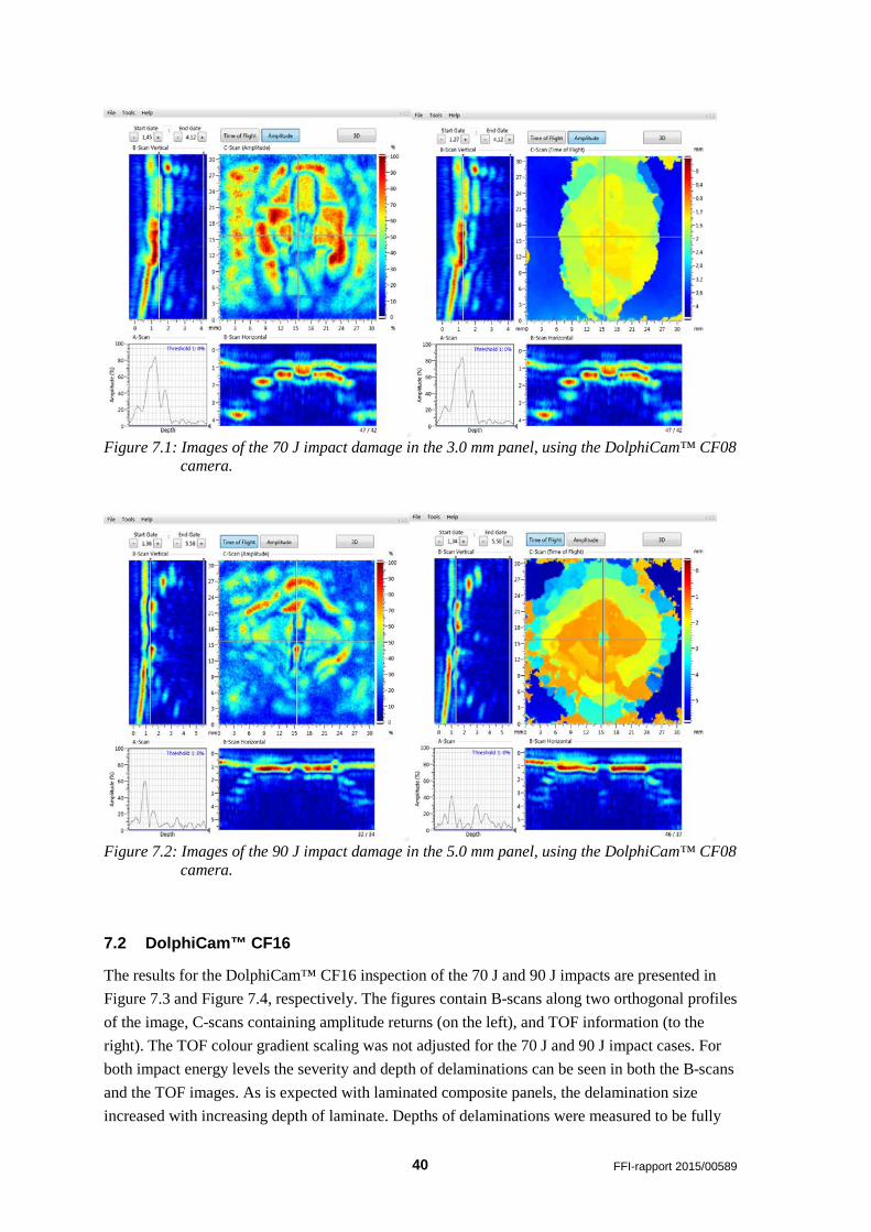
The results for the DolphiCam™ CF08 inspection of the 70 J and 90 J impacts are presented in Figure 7.1 and Figure 7.2, respectively. The figures contain B-scans along two orthogonal profiles of the image, and C-scans containing amplitude returns (on the left) and time of flight (TOF) information (to the right). The TOF colour gradient scaling was not adjusted for the 70 J and 90 J impact cases. For both impact energy levels, the severity and depth of delaminations can be seen in both the B-scans and the TOF images. The images show that the delaminations increase in size as the damage propagates deeper into the CFRP panel. The 3.0 mm thick panel with impact energy 70 J contains delamination damage throughout the thickness, while the 5.0 mm panel delamination damage propagated to a depth of approximately 3.0 mm.


Figure 7.1: Images of the 70 J impact damage in the 3.0 mm panel, using the DolphiCam™ CF08 camera.

Figure 7.2: Images of the 90 J impact damage in the 5.0 mm panel, using the DolphiCam™ CF08 camera.


The results for the DolphiCam™ CF16 inspection of the 70 J and 90 J impacts are presented in Figure 7.3 and Figure 7.4, respectively. The figures contain B-scans along two orthogonal profiles of the image, C-scans containing amplitude returns (on the left), and TOF information (to the right). The TOF colour gradient scaling was not adjusted for the 70 J and 90 J impact cases. For both impact energy levels the severity and depth of delaminations can be seen in both the B-scans and the TOF images. As is expected with laminated composite panels, the delamination size increased with increasing depth of laminate. Depths of delaminations were measured to be fully


through the thickness for the 3.0 mm panel, and at a depth of 3.0 mm for the 5.0 mm panel. The TOF information provided good measurements of delamination size and orientation in the various panel plies.

Figure 7.3: Image of the 70 J impact damage in the 3.0 mm panel, using DolphiCam™ CF16.

Figure 7.4: Image of the 90 J impact damage in the 5.0 mm panel, using the DolphiCam™ CF16 camera.

7.3 Omniscan MX

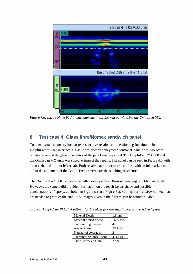
The results from a linear encoded Omniscan MX scan for the 70 J and 90 J impacts are presented in Figure 7.5 and Figure 7.6, respectively. The images show a B-scan and C-scan image of each damage location. The C-scan images of the impact delamination damages provide good measurements of the total delamination area and shape. However, the individual ply


delaminations are difficult to differentiate. The Omniscan MX displays the B-scan image for one selected profile, which can be adjusted during and after the completion of the scan. This helps to determine if the displayed signal returns are delamination features or secondary reflections resulting in false returns. The depth of damages was measured to be 3.0 mm for both the 3.0 mm and 5.0 mm thick panels.

Figure 7.5: Image of the 70 J impact damage in the 3.0 mm panel, using Omniscan MX.


Figure 7.6: Image of the 90 J impact damage in the 5.0 mm panel, using the Omniscan MX.

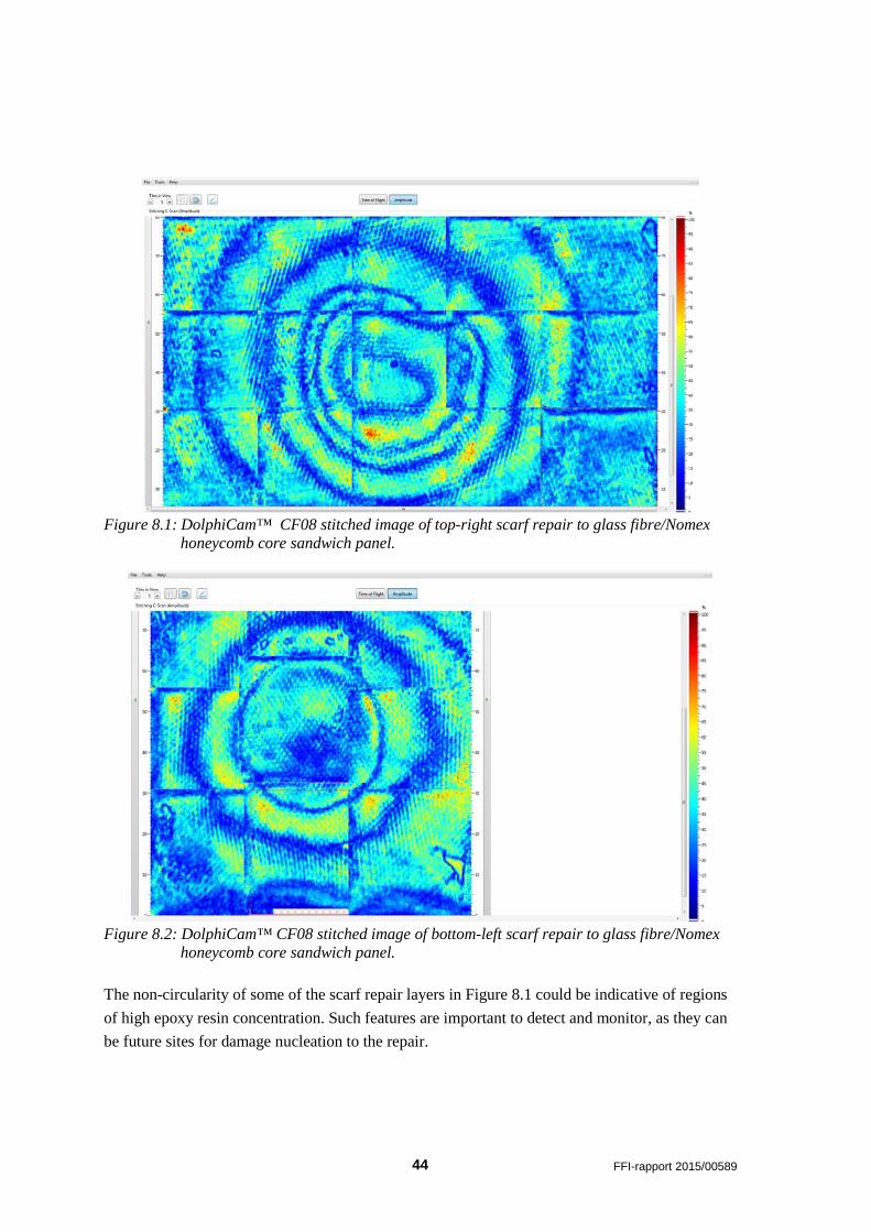
8 Test case 4: Glass fibre/Nomex sandwich panel To demonstrate a cursory look at representative repairs, and the stitching function in the DolphiCam™ user interface, a glass fibre/Nomex honeycomb sandwich panel with two scarf repairs on one of the glass fibre skins of the panel was inspected. The DolphiCam™ CF08 and the Omniscan MX units were used to inspect the repairs. The panel can be seen in Figure 4.5 with a top-right and bottom-left repair. Both repairs have a dot matrix applied with an ink marker, to aid in the alignment of the DolphiTech cameras for the stitching procedure. The DolphiCam CF08 has been specially developed for ultrasonic imaging of CFRP materials. However, the camera did provide information on the repair layers shape and possible concentrations of epoxy, as shown in Figure 8.1 and Figure 8.2. Settings for the CF08 camera that are needed to produce the amplitude images given in the figures, can be found in Table 1.

Table 1: DolphiCam™ CF08 settings for the glass fibre/Nomex honeycomb sandwich panel.

Material Depth 1.9mm Material Sound Speed 1600 m/s Transmitting Elements 4 Analog Gain 39.1 dB Number of Averages 2 Transmitting Pulse Shape 4 (CF04) Time Corrected Gain None


Figure 8.1: DolphiCam™ CF08 stitched image of top-right scarf repair to glass fibre/Nomex honeycomb core sandwich panel.

Figure 8.2: DolphiCam™ CF08 stitched image of bottom-left scarf repair to glass fibre/Nomex honeycomb core sandwich panel. The non-circularity of some of the scarf repair layers in Figure 8.1 could be indicative of regions of high epoxy resin concentration. Such features are important to detect and monitor, as they can be future sites for damage nucleation to the repair.


In Figure 8.3, the Omniscan MX imagery of the bottom-left scarf repair in the glass fibre/Nomex honeycomb sandwich panel is shown. Ultrasonic imaging of the glass fibre scarf repair shows that it is possible to detect the different layers of the patch with the amplitude information.

Figure 8.3: Omniscan MX A-scan and C-scan imagery of the bottom-left scarf repair of the glass fibre/Nomex honeycomb sandwich panel.

9 Discussion and conclusion The DolphiCam™ CF08 and DolphiCam™ CF16 demonstrated the ability to detect simulated delaminations, impact, and borehole features in monolithic CFRP panels. Both DolphiCam™ models could image inclusion defect details, such as waviness as shown in Figure 6.12, and impact damage features as shown in Figure 7.2. Throughout the range of investigated defects, the two cameras performed identically, with the only exception being that at depths where the composite thickness was over 8 mm thick, the CF08 camera was unable to detect features. All inspections performed with the DolphiTech cameras were done without the use of water or gel as a coupling medium between the test panel and transducer pad. The CF16 and CF08 camera inspections taken indoors at an ambient temperature of about 23o C, were compared to tests performed at temperatures of o3 C− . With a quick calibration performed to adjust for system temperature changes, there was no discernable effect to the CF16 and CF08 performance. When it is expected that irregularities or damages will exist in the far-field region of the composite, the use of Time of Flight (TOF) has been found to be very useful for quickly


identifying all simulated damage types. The colour gradient scale for many TOF investigations of defects was adjusted in the DolphiCam interface to provide better discrimination between features with similar depths. This adjustment is visible in Figure 6.20. An example of how the TOF image clearly shows a blind hole can be seen in the right of Figure 5.5, compared to the weak amplitude image given in the left of the figure. However, the opposite was often found to be true for inspections of depths closer to the composite panel surface, known as the near-field. The use of amplitude signals provided clearer imagery of simulated defects. This is evident in Figure 6.1, where the 0.5 mm deep rectangular aluminium inclusion is investigated. Here, the TOF image provides less contrast due to the physical constraints. For operators of ultrasonic imaging systems it is important to recall the trade-off in image quality dependent on depth and use of amplitude or TOF. Both the DolphiCam™ CF08 and DolphiCam™ CF16 excelled when detailed inspections of features are required. For example, the 5 mm deep single layer Teflon® inclusion exhibits a feature that is visible in both the amplitude and TOF imagery. This feature was detected with both the CF08 and CF16 cameras as shown in both Figure 6.6 and Figure 6.18, respectively. While the exact cause for the feature seen in the 5 mm deep inclusion is unknown, it can be used as an example of the DolphiTech cameras’ ability to inspect bonded repair type systems for defects. X-ray imagery, to determine the actual source of the ultrasonic signal returns, is recommended for further study of these unknown features. The existence of signal reflections was seen for both the two DolphiTech systems and the Omniscan MX. The CF16 imagery of an aluminium disk inclusion at 1 mm deep clearly shows the existence of signal reflections, as was typical of DolphiCam™ images in the near-field. The physics of ultrasonic inspection causes these signal reflections to be recorded as false returns that can be misleading if not properly understood by the operator. The Omniscan MX system also exhibited strong signal reflection and false return artefacts from simulated defects, as shown in Figure 6.26 for the image of the rectangular aluminium inclusions. The DolphiCam™ CF08 and DolphiCam™ CF16 both provided very detailed imagery of the delaminations caused by impacts, as seen in Figure 7.2 and Figure 7.4. The performances of the two cameras are qualitatively similar up to the design depth of the CF08 camera. Depths and areas of individual lamina delaminations can be very accurately determined. Also, the conical expansion of the delamination damage is visible in the side profiles and TOF images. The diamond shapes of the delaminations are coincident with lamina fibre direction. The performance of the two DolphiTech systems differed when the glass fibre/Nomex honeycomb sandwich panel was inspected. While both the DolphiCam™ CF08 and DolphiCam™ CF16 are specifically designed for inspection of carbon fibre composites, it has been found that limited inspection of other composite materials is possible with the proper adjustment of system settings. Only the CF08 camera was able to image the scarf repairs of the glass fibre sandwich, as seen in the stitched imagery of Figure 8.1 and Figure 8.2. The very thin (~1.0 mm) and low density glass fibre skin is challenging to image, as much of the signal is


attenuated and refracted. Despite the imaging challenges posed by the glass fibre material, the different layers of the scarf repairs, as well as regions of high resin concentrations, are visible. The Olympus Omniscan MX system is a highly versatile system that can be configured to inspect many different materials and geometries. Imaging large planar areas with the Omniscan MX is quite fast, with scans of 420 mm x 64 mm to be completed in less than one minute after the system is set up. The Omniscan system does, however, require a bit more equipment than the DolphiTech cameras, as seen when comparing the system set-ups in Figure 3.1 and Figure 2.1, respectively. The Omniscan MX also requires a fluid couplant flow, which limits the system operation to above-freezing ambient temperatures, and more often to depot maintenance environments. While mobile, the Omniscan MX and associated equipment is not handheld, and can take a number of minutes to pack, transport, and set up. The Omniscan MX system performed very well at detecting all the simulated defects rapidly and with ease, over large relatively horizontal areas. An example is the inspection of the circular aluminium inclusions in Figure 6.26. Here, the Omniscan MX was able to detect all the inclusions quickly with no a priori knowledge of their location, as can be required by the comparatively smaller scan area (30 mm x 30 mm) of the DolphiTech cameras. The Omniscan system trades quick detectability for detailed inspection of the damaged areas. This is evident when comparing the scans of the impact damaged areas with those from the DolphiTech cameras. For example, the 90 J impact case shown in Figure 7.6, as imaged by the Omniscan MX, lacks some of the detail of the DolphiCam™ CF16 scan, as shown in Figure 7.4. The DolpiCam™ CF16 provides better measurement of delamination depth and damage form. However, the approximate size of the total damage area can be measured with the Omniscan MX system. The Omniscan MX scan does not provide the same level of detail for the repair sections as the DolphiCam™ CF08. In the image of the repair patch in Figure 8.1, areas of discontinuity are observed. These are possibly regions of high resin concentration. Such detailed information is very useful for post repair inspection and validation, as well as monitoring of patch performance over time. As a conclusion, all three systems, i.e. DolphiCam™ CF08, DolphiCam™ CF16, and Olympus Omniscan MX, could detect all the simulated damages within their design profiles. The Omniscan MX system is very flexible, but requires more support equipment and training to operate effectively when compared to the DolphiTech cameras. On the contrary, the Omniscan MX can quickly scan very large areas, which are useful when doing a broad sweep inspection of aircraft structures. The ability to use many different specialized transducers with the Omniscan MX make it highly versatile. However, for this study of horizontal plates, the wedge and VersaMOUSE were the most appropriate. The inspection quality of the CFRP panels was identical for the two DolphiCam™ cameras up to the design range of the CF08 camera. The CF08 camera performed best of the three systems when inspecting glass fibre skin/Nomex core sandwich repairs. However, this type of composite is outside the original design range of the instrument.


It is recommended that a combined use of the Olympus Omniscan MX and DolphiCam™ CF16 be employed for aircraft composite structure inspection. The Omniscan MX will provide excellent damage detection for the simulated damages in this study in a depot maintenance environment, while the DolphiCam™ CF16 is excellent for forward “field use” inspection of areas that are known to be damaged.

Acknowledgements The authors would like to thank Torbjørn Olsen for useful input and contribution to the inspection work and the final version of this report, and Bernt Brønmo Johnsen for comments to the final version of this report. We would also thank DolphiTech for letting us try out the DolphiCam™CF16 camera.


Vedlegg A User’s Guide to Olympus Onmiscan MX

A.1 Introduction

This guide is a quick guide for using the Olympus Omniscan MX to do a simple C-scan. This guide is based on the user’s manuals for Omniscan MX equipment, which can be found digitally in the product manuals for the Omniscan MX and VersaMOUSE.

A.2 Basic Set-up

To perform a C-scan, the Omniscan MX unit, probe, and VersaMOUSE are needed. It is also helpful to use a keyboard and mouse with the Omniscan MX to make navigation in the menus and entering in values easier. An overview of the Omniscan MX unit and its control buttons is given in Figure 9.1 . Before turning on the system, make sure to connect the various parts of the system together as shown in Figure 9.2. The Omniscan MX cables and ports are unique to each piece of equipment, so it is designed to be easy to set up. If it fits in the port, it is the correct cable for that port.

Figure 9.1: Omniscan MX control buttons.


(a) (b)

Figure 9.2: Set-up configuration (a) and cable connections (b) for the Olympus Omniscan MX.

The ultrasonic probe requires a connecting fluid for the waves to pass through from the probe to the material to be inspected. For most scans, water is all that is required. This can be delivered from a small bottle to the wedge, as shown in Figure 9.2a. For some applications, a small amount of gel along with the water will improve the obtained images. Figure 9.3 shows the ultrasound probe, the wedge, and the VersaMOUSE; the VersaMOUSE is also shown in Figure 9.7. The probe is mounted on top of the wedge, which is connected with a correct amount of water flow. Too much water on the panel surface will cause the encoder wheels of the VersaMOUSE to slip, resulting in false distance measurements. If this occurs, simply wipe the water away, and restart the scan for the area in question.

Figure 9.3: The probe is mounted on top of the wedge. The water flow is delivered to the wedge from the tube couplings. The wedge and the probe is connected to the VersaMOUSE.


The hardware is now ready for performing a C-scan. In addition, it is important to ensure that the correct set-up file for the material is selected in the software system. If you are unsure that the correct set-up file is selected, or if you need to calibrate the speed of sound for a material, see Section A.3. Otherwise, proceed to Section A.4.

A.3 Calibrating Material Speed of Sound

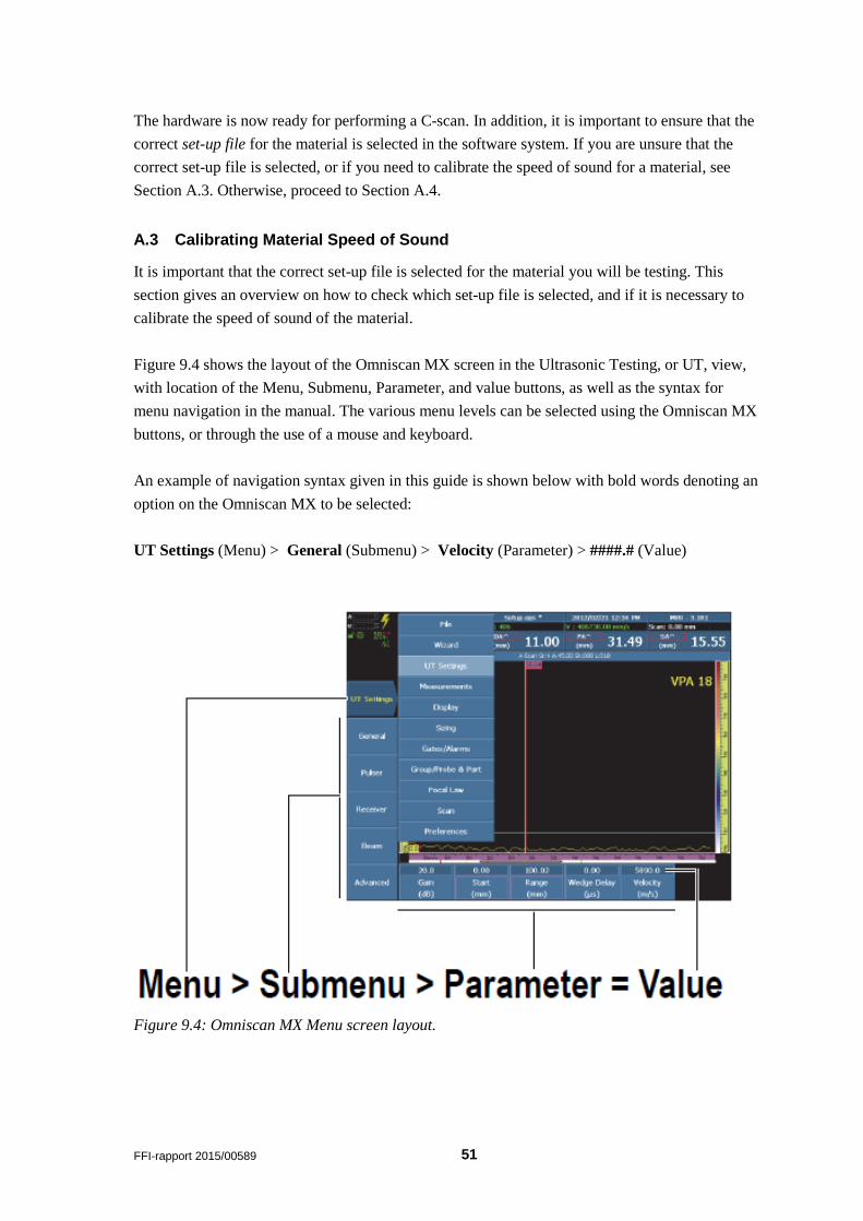
It is important that the correct set-up file is selected for the material you will be testing. This section gives an overview on how to check which set-up file is selected, and if it is necessary to calibrate the speed of sound of the material. Figure 9.4 shows the layout of the Omniscan MX screen in the Ultrasonic Testing, or UT, view, with location of the Menu, Submenu, Parameter, and value buttons, as well as the syntax for menu navigation in the manual. The various menu levels can be selected using the Omniscan MX buttons, or through the use of a mouse and keyboard. An example of navigation syntax given in this guide is shown below with bold words denoting an option on the Omniscan MX to be selected: UT Settings (Menu) > General (Submenu) > Velocity (Parameter) > ####.# (Value)

Figure 9.4: Omniscan MX Menu screen layout.


To check the set-up file, navigate to File > Open Here you will see a list of the saved .ops files in the unit. Clicking a file and selecting Open will load that set-up file. If there does not exist a set-up file for the type of material you are testing, the following procedures explain how to calibrate the speed of sound for a new material, and to save it as a set-up file for future use. Note that to calibrate the speed of sound for a new material you will need two different and known thicknesses of the material. Calibration blocks, or two panels of different thicknesses will work, such as shown in Figure 9.5.

The procedure is as follows:

1. Ensure that the correct wedge is selected in the system settings, Probe/Part> Select> Wedge> ”choose”,

2. Choose Wizard> Calibration> Type = Ultrasound

3. Choose Wizard> Calibration> Mode = Velocity

4. Choose Wizard> Calibration> Start

5. In Select A-Scan

6. Choose reference VPA for calibrating.

7. It is important to use the thinner panel as Thickness 1, and the thicker panel as Thickness 2 (according to Olympus recommendations). Shift the probe from one panel to the other, and adjust the Start and Range parameters, such that the signals from the surface, as well as back walls for both panels can be seen; see Figure 9.6. As a reference for adjustment: If you have a Thickness 2 that is 10 mm, it is likely that your Range will be about 12mm, such that both the surface and back wall signals are visible on the screen.

Probe

Wedge

Probe

Wedge

Thickness 1 Thickness 2

Figure 9.5: Two panels with known thickness.


Figure 9.6: Signals from the surface and back wall of a panel.

8. Adjust Gain such that the signal for the back wall of Thickness 1 is at 80%

9. Choose Next

10. In Radius 1 and Radius 2, choose Echo Type = Thickness

11. Choose Thickness 1 and enter in the known thickness of panel 1.

12. Choose Thickness 2 and enter in the known thickness of panel 2.

13. Next

14. Set the Probe on panel 1 and in Set Gate A on Thickness 1, adjust the Start and Width values such that the edges of Gate A (red) are on either side of the signal.

15. Adjust the Threshold to 25%

16. Choose Get Position

17. Set the Probe on panel 1 and in Set Gate A on Thickness 2 adjust the Start and Width values such that the edges of Gate A (red) are on either side of the signal.

18. Adjust the Threshold such that the signal crosses the Gate.

19. Choose Get Position

20. Choose Accept if you agree with Material Velocity, or choose Restart. An average value for aerospace monolithic carbon fiber is 3200 m/s. 21. Save the new material velocity as a setup file in the Omniscan MX for future use. Select File > Save Setup As, and enter in a desired file name.

A.4 C-scan with VersaMOUSE

To use the positioning system as part of the scan set-up, connect the wedge, probe and VersaMOUSE together as is shown in Figure 9.7. Recall that adequate coupling fluid flow is needed for good signal return.


Figure 9.7: Performing a C-scan with VersaMOUSE.

Choose Scan> Inspection> Type = Raster Scan When the versaMOUSE is connected, and a Raster Scan selected, the Omniscan MX display will show the A-scan and the C-scan images as default. If you would like to view other display options, you can switch between a list of pre-defined displays: Display > Display = “choose desired setting” To begin or reset a scan simply choose Scan > Start

A.5 Creating a Report

To create a report of the current scan data, first set the storage location. File > Storage If the storage location will be a USB memory stick, ensure that before the Omniscan MX is powered on, the USB memory stick is placed into one of the available USB ports. To create the report: File > Report > File Name = “choose report name” Type in the desired name for the report, and select Build. The report and images are now saved in the selected storage location. More detailed information on creating or modifying report formats can be found in the Omniscan MX Software User’s Manual, page 34.


A.6 File transfer to USB

To transfer reports, scan files, or set-up files from the Omniscan MX to a USB, first ensure that after the system has booted up, the USB is recognized: File > Storage This will display the available storage options for the Omniscan MX; Storage Card *\Storage Card*, Internal Memory *\User*, and USB Storage *\Hard Disk*. To maintain the default setting of storing all report and scan data on the SD storage card select, File > Storage > Storage Card This also selects the location from which files will be transferred. To transfer Data files, Set Up files, and generated Reports select Preferences > Service > File Manager The left window displays the files that are stored in the set storage location from above. You can filter by file type, or simply display All files. The right window is the destination location for the file transfer. For transfers to the USB ensure that *\Hard Disk\* is selected in the destination window. To transfer files, select the desired files, and click Copy. It is important to remember that when transferring a report file to transfer both the .htm file and the associated report folder with the same name. The images from the report are contained in the report folder.


References

[1] T. Olsen, T. Thorvaldsen, and B. B. Johnsen, "Experiences from practical use of ultrasound non-destructive inspection techniques," FFI-rapport 2012/01577 (Fortrolig), 2012.

[2] T. Thorvaldsen, M. Kvalbein, B. B. Johnsen, and T. Olsen, "Thermography and ultrasound as non-destructive inspection techniques," FFI-rapport 2012/01575 (Fortrolig), 2012.

[3] T. Thorvaldsen, B. B. Johnsen, and T. Olsen, "Non-destructive testing of composite materials for military applications," NATO STO AVT-224, 2013.

[4] "DolphiTech AS, www.dolphitech.com," 2015.

[5] "High Performance Composites, www.hpcomposites.no," 2012.

[6] "Product data for HexPly 6376 175C curing epoxy matrix; http://www.hexcel.com/Resources/DataSheets/Prepreg-Data-Sheets/6376_eu.pdf," Hexcel Corporation, 2007.

http://www.dolphitech.com,/

http://www.hpcomposites.no,/

http://www.hexcel.com/Resources/DataSheets/Prepreg-Data-Sheets/6376_eu.pdf,

Tyler P. Jones and Tom Thorvaldsen - FFI · Tyler P. Jones and Tom Thorvaldsen Norwegian Defence...

Documents

Transcript of Tyler P. Jones and Tom Thorvaldsen - FFI · Tyler P. Jones and Tom Thorvaldsen Norwegian Defence...