Two Uniform Tailored Finite Point Schemes for the Two...

Acknowledgments

H. Han is supported by the NSFC Project No. 10971116. M. Tang is supported by NaturalScience Foundation of Shanghai under Grant No. 12ZR1445400 and Shanghai PujiangProgram 13PJ1404700. W. Ying was supported in part by the National Natural ScienceFoundation of China under Grant DMS–11101278 and the Young Thousand Talents Pro-gram of China.

Two Uniform Tailored Finite Point Schemes

for the Two Dimensional Discrete Ordinates Trans-

port Equations with Boundary and Interface Layers

Houde Han1,Min Tang2 ∗, and Wenjun Ying2

1 Department of Mathematical Sciences, Tsinghua University, Haidian, Beijing 100084,P. R. China2Department of Mathematics, Institute of Natural Sciences and MOE-LSC, ShanghaiJiao Tong University, Minhang, Shanghai 200240, P. R. China

Abstract. This paper presents two uniformly convergent numerical schemes for thetwo dimensional steady state discrete ordinates transport equation in the diffusiveregime, which is valid up to the boundary and interface layers. A five-point node-centered and a four-point cell-centered tailored finite point schemes (TFPS) are in-troduced. The schemes firstly approximate the scattering coefficients and sources bypiecewise constant functions and then use special solutions to the constant coefficientequation as local basis functions to formulate a discrete linear system. Numerically,both methods can not only capture the diffusion limit, but also exhibit uniform conver-gence in the diffusive regime, even with boundary layers. Numerical results show thatthe five-point scheme has first-order accuracy and the four-point scheme has second-order accuracy, uniformly with respect to the mean free path. Therefore a relativelycoarse grid can be used to capture the two dimensional boundary and interface layers.

AMS subject classifications: 65L12, 76N20, 35Q70

Key words: Neutron transport equation, discrete ordinates method, tailored finite point method,boundary layers, interface layers.

∗Corresponding author. Email addresses: [email protected] (Houde Han), [email protected](Min Tang), [email protected] (Wenjun Ying)

http://www.global-sci.com/ Global Science Preprint

2

1 Introduction

The neutron or radiative transport equation is widely used in nuclear engineering, ther-mal radiation transport, charged-particle transport and oil-well logging tool design, etc..Developing efficient numerical methods for the neutron transport equation has been anactive area for decades [20–22].

The solutions of the neutron transport equation depend on space, time, and velocities,which require a lot of computational cost for simulations. The discrete ordinates versionof the steady state neutron transport equation is a semi-discretization in velocity. Startingfrom the discrete ordinates methods, which are among the most popularly used methodsin the community, various space discretizations are investigated in the last two decades.For example, the diamond-difference method [22], the characteristic method [3, 7], thediscontinuous finite element method [1, 27], the nodal method [2, 21], and so on.

When the average distance between two successive collisions (the mean free path) ǫis small, it is generally impossible to accurately solve the discrete ordinates transportequation in the diffusive regime by optically thin (∆x ≪ ǫ) meshes, because of limits incomputer memory. To approximate the solutions, some macroscopic models have beenderived by asymptotic analysis [19], for example, the optically thin limit, the opticallythick absorptive limit and the optically thick diffusive limit [20]. Here in this paper, wefocus ourselves on the diffusive regime. Two criteria for designing accurate space dis-cretizations for the discrete ordinates transport equation are 1) the order of their trunca-tion error which guarantees the convergence and accuracy in the optically thin regime;2) the discretization should converge to a discretization of the diffusion limit equation asthe mean free path tends to zero [17, 18]. This gives the accuracy with optically thick cell(∆x≫ǫ) of a transport spatial discretization.

The idea of using unresolved cells to capture the macroscopic limit model has been suc-cessfully extended to more general applications, which is called asymptotic preservingschemes [8]. However the asymptotic preserving property only guarantees the accuracyof the diffusive region away from the boundary layer. One important issue is the schemebehavior in the presence of unresolved boundary/interface layers. In many applications,if a diffusive region is adjacent to a transport region, boundary and interface layers mayappear. Flux changes rapidly across the boundary/interface layers, which requires suffi-ciently fine grids to capture these changes. It is usually impractical to prescribe a spatialgrid that adequately resolves all boundary/interface layers. Therefore, it is desirable todesign numerical schemes that are accurate across the boundary/interface layers, even ifthe spatial grids are not fine enough to resolve the fast variations.

The known schemes for the neutron transport equation that can capture the boundarylayers with coarse meshes (meshes that do no resolve the fast variation) are restrictedto the one dimensional case. For example, the spectral nodal method proposed in [5, 9],the domain decomposition method in [10] and the micro-macro decomposition methoddiscussed in [23]. These methods are shown to be valid up to the boundary even if theboundary layers exist, but only in one dimension. Though higher dimensional extensions

3

have been investigated in [2,5,26], the additional approximations for the transverse leak-age terms make these higher dimensional extensions no longer able to accurately capturethe fast changes in the boundary layers.

The difference between one and high dimensional boundary layer analysis is that, inone space dimension, the solutions change fast in one direction and it is possible to ex-press the solution by a finite number of basis functions, while in higher dimensions, thesolutions vary fast in infinite number of directions and have infinite number of basis func-tions for the general solutions. This makes the high dimensional boundary layer analysisand simulations much harder than the one dimensional case. To the best of authors’knowledge, there exists no numerical method for the neutron transport equation that cancapture the high dimensional boundary and interface layers with coarse meshes [20].

In this paper, we construct two new space discretizations for the two dimensionalsteady state discrete ordinates transport equation with discontinuous coefficients, which,by using coarse meshes, can capture not only the diffusion limit in the diffusive region butalso the fast changes in the boundary/interface layers. The idea is to use the tailored finitepoint method that was proposed by Han, Huang and Kellogg [14, 15] for the numericalsolutions of singular perturbation problems of second order elliptic equations with con-stant coefficients. The basic idea of the tailored finite point method is that the numericalscheme is tailor-made at each point, based on the local properties of the solutions. Sincethis method makes full use of the analytical property of the local solutions, it can cap-ture the boundary layers even with coarse grids. Later on, Han and Huang [11–13] andShih, Kellogg et al. [24, 25] systematically extend this method for the nonhomogeneousreaction-diffusion, convection-diffusion and convection-diffusion-reaction problems.

In this work, we focus on the isotropic scattering case with discontinuous coefficients,where the total cross section, the macroscopic scattering cross section and the neutronsource are all isotropic in velocity and piecewise smooth in space. The remainder of thispaper is organized as follows. In section 2, we give a brief introduction of the neutrontransport equation, its diffusion limit and the discrete ordinates equations. In section3, we discuss about the homogeneous discrete ordinates equations with constant coeffi-cients and its special solutions, which are used as local basis functions in the constructionof TFPS. A five-point node-centered TFPS and a four-point cell-centered TFPS, are de-scribed in section 4. In section 5, some numerical examples are presented to demonstratetheir uniform convergence when the boundary/interface layers exist and ability to cap-ture the boundary/interface layers. Finally, we conclude with a discussion in section6.

2 The two dimensional discrete ordinate transport equation

2.1 The two dimensional neutron transport equation

When particles in a bounded domain interact with a background through absorption andscattering processes, the density function is governed by the linear neutron transport

4

equation.

The steady state isotropic neutron transport equation reads [22]:

ǫu·∇ψ(z,u)+σT(z)ψ(z,u)=1

4π

(

σT(z)−ǫ2 σa(z))

∫

Sψ(z,u)du+ǫ2 q(z), (2.1)

subject to the boundary conditions

ψ(z,u)=ψ−Γ (z,u), for z∈Γ−

u =z∈Γ=∂Ω : u·nz <0, u∈S. (2.2)

Here z∈Ω⊂R3 is the space variable, nz is the outward normal vector and S= v|v∈R3,|v|= 1 represents the directions of particle velocities. ψ(z,u) is the density of theparticles moving in direction u∈ S at position z. ǫ is a dimensionless parameter that isgiven by the ratio of the mean free path describing the average distance between twosuccessive collisions and the typical length scale. The quantities, σT/ǫ, ǫσa and ǫq, arethe total cross section, absorption cross section and source respectively, in which σT(z),σa(z) and q(z) are piecewise smooth whose values are bounded and in dependent of ǫand the L∞ norm of their derivatives ∇σT(z), ∇σa(z) and ∇q(z) are also bounded andindependent of ǫ, except at the interfaces. ψ−

Γ (z,u) is a given function on Γ−u ×S, which

specifies the particle densities that come into the computational domain.

Interface conditions are needed to determine the unique solution. Assume that theparticles do not change their directions when passing through the interfaces of differentmedia, which indicates that, at the interfaces, the coefficients σT, σa and q may have dis-continuities, but ψ(z,u) is continuous. For any interface line α, let the two different mediabe denoted by + and −, we have

ψ+∣

∣

α=ψ−∣

∣

α. (2.3)

The neutron transport equation (2.1) is a six-dimensional equation in the space vari-ables z∈R3 and directions u∈S. It can be reduced to lower dimensional equations. Inthe Cartesian coordinate system, let

u=(c,s,ζ)

with

c=(1−ζ2)12 cosθ and s=(1−ζ2)

12 sinθ for |ζ|≤1.

The neutron transport equation (2.1) has the form

ǫ

(

c∂ψ

∂x+s

∂ψ

∂y+ζ

∂ψ

∂z

)

+σT(x,y,z)ψ

=1

4π

(

σT(x,y,z)−ǫ2 σa(x,y,z))

∫ 2π

0

∫ 1

−1ψ(

x,y,z,c,s,ζ)

dζdθ+ǫ2 q(x,y,z)

. (2.4)

5

Suppose that σT, σa, q only depend on x, y and ψ is uniform along the z axis. Thefunction

ψ(x,y,ζ,θ) =1

2

[

ψ(x,y,z,c,s,ζ)+ψ(x,y,z,c,s,−ζ)]

is independent of z and an even function in ζ. The equation (2.4) is reduced to a twospace dimensional neutron transport equation

ǫ

(

c∂ψ

∂x+s

∂ψ

∂y

)

+σT(x,y)ψ

=1

2π

(

σT(x,y)−ǫ2 σa(x,y))

∫ 2π

0

∫ 1

0ψ(x,y,c,s)dζdθ+ǫ2 q(x,y) (2.5)

for ψ(x,y,ζ,θ), in which c2+s2≤1.

In the case that the boundary condition function ψ−Γ (z,u)=ψΓ(z) is independent of u,

when the collisions between particles are frequent (ǫ→ 0), the solution of (2.1) becomesisotropic in u and can be approximated by the solution of the diffusion equation

−∇·( 1

σT∇φ)

+σa φ=q, (2.6)

subject to the boundary condition

φ(z)=ψΓ, for z∈Γ. (2.7)

In two space dimensions, the diffusion limit equation corresponding to (2.5) takes theform:

− ∂

∂x

(

2

3σT

∂φ

∂x

)

− ∂

∂y

(

2

3σT

∂φ

∂y

)

+σaφ=q. (2.8)

The diffusion limit equation can be derived by the Chapman-Enskog expansion as dis-cussed in [19]. The calculations are straightforward and we omit the details here. Notethat being isotropic in u implies different physical settings in the two transport equation(2.1) and (2.5), which causes the different coefficients in the elliptic operators in (2.6) and(2.8).

2.2 The discrete-ordinate transport equations

The idea of the discrete ordinate method is to approximate the integral in the originaltransport equation (2.4) by numerical quadrature set [22]. In the two dimensional equa-tion (2.5), let the discrete points be (ζm,θm)m∈V with weights wmm∈V . Here, V repre-sents the index set. Let cm=(1−ζ2

m)1/2cos(θm) and sm=(1−ζ2

m)1/2sin(θm) with ζm∈[0,1].

We represent the quadrature set by cm,sm,wmm∈V .

6

The discrete-ordinate form of (2.5) by the quadrature set reads

ǫ(

cm∂

∂xψm+sm

∂

∂yψm

)

+σTψm =(

σT−ǫ2 σa

)

∑n∈V

ψnwn+ǫ2 q, m∈V, (2.9)

with ψm =ψm(x,y) be an approximation of the density function ψ(x,y,ζm,θm) for m∈V.For simplicity, we assume that the spatial variables x∈(0,a) and y∈(0,b) with two positivereal numbers a and b. Let rectangle

D=(x,y)∣

∣x∈ (0,a), y∈ (0,b)be the computational domain, in which the discrete-ordinate equation (2.9) holds. Onthe boundary ∂D, the approximate particle density functions ψm(x,y)m∈V satisfy theboundary conditions (2.2), which now take the form, for x∈ [0,a] and y∈ [0,b],

ψm(0,y)=ψLm(y), cm >0; ψm(a,y)=ψRm(y), cm<0;ψm(x,0)=ψBm(x), sm >0; ψm(x,b)=ψTm(x), sm <0.

(2.10)

Here, ψBm(x), ψTm(x), ψLm(y) and ψRm(y) (m ∈ V) are known functions. The interfaceconditions corresponding to (2.3) become

ψ+m

∣

∣

α=ψ−

m

∣

∣

α, m∈V. (2.11)

In order to have the discrete-ordinate equations (2.9) converge to the same diffusionlimit equation (2.8), as ǫ tends to zero (when the boundary conditions are independent ofm), the quadrature set cm,sm,wmm∈V is required to satisfy the condition [26]

∑n∈V

wn=1, ∑n∈V

wncn =0, ∑n∈V

wnsn =0,

∑n∈V

wncnsn =0, ∑n∈V

wn(c2n+s2

n)=23 .

(2.12)

This can be obtained by similar Chapman-Enskog expansions as in the derivation of thediffusion limit equation.

Let M be a positive integer and V = 1,2,··· ,··· ,4M be the index set. We choose asymmetric quadrature set cm,sm,wm by assuming

wm=wm+M=wm+2M=wm+3M>0, m=1,··· ,Mθm = θm+M− π

2 = θm+2M−π= θm+3M− 32 π∈ (0, π

2 ), m=1,··· ,Mζm = ζm+M = ζm+2M = ζm+3M ∈ [0,1], m=1,··· ,M

cm =(1−ζ2m)

12 cosθm, sm =(1−ζ2

m)12 sinθm, m∈V.

(2.13)

The requirement (2.12) indicatesM

∑n=1

wn(1−ζ2n)=

16 and further

M

∑n=1

wn ζ2n =

1

12. (2.14)

7

We can check that when the set cm,sm,wm are chosen by (2.13)-(2.14), the requirement(2.12) is satisfied, so that the discrete-ordinate system possesses the same diffusion limitas the original integral equation.

In this paper, we consider the most commonly used Gaussian quadratures set

SN =cm,sm,wmm∈V

with N a positive integer parameter [22]. In a quadrature set SN , each quadrant hasM= N(N+1)/2 ordinates and N distinct ζm ∈ (0,1), which are the positive roots of thestandard Legendre polynomial of degree 2N on interval [−1,1]. We display the corre-sponding cm, sm, wm for S1, S2, S3, S4. It is easy to check that the Gaussian quadraturessatisfy (2.13)-(2.14).

• Quadrature set S1: When N=1 and M=N(N+1)/2=1, ζ21 =1/3, θ=π/4, then

(c1,s1)=

(√3

3 ,√

33

)

, (c2,s2)=

(

−√

33 ,

√3

3

)

,

(c3,s3)=

(

−√

33 ,−

√3

3

)

, (c4,s4)=

(√3

3 ,−√

33

)

,

w1=w2=w3=w4=14

• Quadrature set S2: When N=2 and M=N(N+1)/2=3, the quadrature nodes andweights of the quadrature set S2 are presented in Table 1

Table 1: The nodes and weights of the quadrature set S2.

ζm θm cm sm 4wm

0.3399810 π/8 0.8688461 0.3598879 0.3260726

0.3399810 3π/8 0.3598879 0.8688461 0.3260726

0.8611363 π/4 0.3594748 0.3594748 0.3478548

• Quadrature set S3: When N=3 and M=N(N+1)/2=6, the quadrature nodes andweights of the quadrature set S3 are presented in Table 2

• Quadrature set S4: When N = 4 and M = N(N+1)/2= 10, the quadrature nodesand weights of quadrature set S4 are presented in Table 3.

SN(N=1,2,3,4) satisfy not only the requirement (2.13)-(2.14), but also

wm=wM−m, θm+θM−m=π

2, m=1,··· ,M, (2.15)

which introduces additional symmetries.

8


ζm θm cm sm 4wm

0.2386192 π/12 0.9380233 0.2513426 0.1559713

0.2386192 3π/12 0.6866807 0.6866807 0.1559713

0.2386192 5π/12 0.2513426 0.9380233 0.1559713

0.6612094 π/8 0.6930957 0.2870896 0.1803808

0.6612094 3π/8 0.2870896 0.6930957 0.1803808

0.9324695 π/4 0.2554414 0.2554414 0.1713245


ζm θm cm sm 4wm

0.1834346 π/16 0.9641432 0.1917800 0.0906709

0.1834346 3π/16 0.8173612 0.5461433 0.0906709

0.1834346 5π/16 0.5461433 0.8173612 0.0906709

0.1834346 7π/16 0.1917800 0.9641432 0.0906709

0.5255324 π/12 0.8217842 0.2201964 0.1045689

0.5255324 3π/12 0.6015878 0.6015878 0.1045689

0.5255324 5π/12 0.2201964 0.8217842 0.1045689

0.7966665 π/8 0.5584105 0.2313012 0.1111905

0.7966665 3π/8 0.2313012 0.5584105 0.1111905

0.9602899 π/4 0.1972858 0.1972858 0.1012285

3 Special solutions to homogeneous constant coefficients system

In order to apply the tailored finite point method to construct numerical schemes for theboundary value problem (2.9)-(2.11) with variable coefficients, we need to use the specialsolutions to the problem of interest as basis functions. In this section, we will find thespecial solutions to the homogeneous discrete-ordinate equations

ǫ

(

cm∂

∂x+sm

∂

∂y

)

ψm+σTψm=(σT−ǫ2σa) ∑n∈V

ωnψn, m∈V, (3.1)

with constant coefficients σT and σa.

Let

Ψ(x)=(ψ1(x),ψ2(x),··· ,ψ4M(x))T ∈R4M

9

with x=(x,y)∈R2. Now we introduce an auxiliary function

C(x)= ∑n∈V

ωnψn(x)

and rewrite system (3.1) in the following form

(

L 00 1

)(

Ψ(x)C(x)

)

=

(

0 e

wT 0

)(

Ψ(x)C(x)

)

. (3.2)

Here, L is a 4M by 4M diagonal matrix, whose mth diagonal entry reads ǫ(cm∂x+sm∂y)+σT, for m∈V, and vectors e,w∈R4M×1 are respectively given by

e=(σT−ǫ2σa)(1,1,··· ,1)T

andw=(w1,w2,··· ,w4M)T.

The system (3.2) contains (4M+1) unknown functions Ψ(z) and C(z).The two systems (3.1) and (3.2) are equivalent to each other. In the subsequent part, we

are going to find special solutions of the form

(

Ψ(z)C(z)

)

=

(

ξ

η

)

exp

λx+µy

ǫ

(3.3)

to the system (3.2), then the corresponding special solutions to (3.1).In order to determine the nonzero vector ξ =(ξ1,ξ2,··· ,ξ4M)T and scalar constant η as

well as λ and µ, we substitute (3.3) into (3.2). Finding a special solution of the form (3.3)reduces to a matrix eigenvalue problem: find λ,µ∈C and nonzero vector (ξ,η)∈C4M×C

such that(

A 00 1

)(

ξ

η

)

=

(

0 e

wT 0

)(

ξ

η

)

. (3.4)

Here, A=A(λ,µ) is a 4M by 4M diagonal matrix, whose mth diagonal entry reads cmλ+sm µ+σT , for m∈V. We define (λ,µ) as an eigenvalue pair of the problem, if there exists

nonzero solution

(

ξ

η

)

to the system (3.4).

The eigenvalue pairs

Note that the eigenvalue pair (λ,µ) is a zero point of the characteristic polynomial:

p4M(λ,µ)≡det

(

A(λ,µ) −e

−wT 1

)

= ∏m∈V

(cmλ+sm µ+σT)−(σT−ǫ2σa) ∑n∈V

[

ωn ∏m 6=n

(

cmλ+sm µ+σT

)

]

. (3.5)

10

We have eitherπ4M(λ,µ)≡ ∏

m∈V

(cmλ+sm µ+σT)=0, (3.6)

or

q4M(λ,µ)≡1− ∑n∈V

ωn(σT−ǫ2σa)

cnλ+sn µ+σT=0. (3.7)

A few characteristic curves when ǫ = 0.1 for p4M(λ,µ) with M = 1,3,6,10 are shown inFigure 1, where the horizontal and vertical axises represent respectively λ and µ. A pointon the curves corresponds to an eigenvalue pair (λ,µ). Only those eigenvalue pairs ofwhich both λ and µ are real numbers are plotted.

a) b)

c) d)

Figure 1: Characteristic curves when ǫ=0.1: (a) M=1; (b) M=3; (c) M=6; (d) M=10.

The eigenvectors corresponding to (λ,µ)After (λ,µ) is determined, we have to find the eigenvector (ξ,η) associated with theeigenvalue pair.

11

From equation (3.4), we get

(cmλ+sm µ+σT)ξm = (σT−ǫ2σa)η ∀m∈V

η = ∑n∈V

ωn ξn. (3.8)

Case 1. Suppose that cmλ+sm µ+σT 6=0 for all m∈V, then we get

ξm = σT−ǫ2σacmλ+smµ+σT

∀m∈V

η = 1, (3.9)

which is an eigenvector associated with the eigenvalue pair (λ,µ).Case 2. There is at least one m1∈V such that

cm1λ+sm1

µ+σT =0.

Then from (3.8), we obtainη=0,

and further

(cmλ+sm µ+σT)ξm = 0, ∀m∈V, (3.10)

∑n∈V

ωn ξn = 0. (3.11)

By equation (3.10), we know that for any m∈V, we have either ξm=0 or cmλ+sm µ+σT=0.Since ξ is nonzero and satisfies (3.11), there exists another m2∈V such that

ξm2 6=0.

This further indicates thatcm2 λ+sm2 µ+σT =0.

Assume that (cm1,sm1

) and (cm2 ,sm2) are linearly independent and

cmλ+sm µ+σT 6=0 ∀m 6=m1,m2. (3.12)

Then the components of the eigenvector (ξ,η) are given by

ξm =

0 for m 6=m1,m2

wm2 for m=m1

−wm1for m=m2

(3.13)

and

η = 0. (3.14)

12

Now it is clear that after an eigenvalue pair (a zero point (λ,µ) of (3.5)) is found, thecorresponding eigenvector (ξ,η) can be obtained directly.

Properties of the eigenvalue pairs and eigenvectors We have found infinite numberof special solutions in the form (3.3), while the idea of the tailored finite point method isto select a finite number of special solutions and make the discrete scheme satisfy themexactly. We prove in the subsequent part some properties of the eigenvalue pairs andtheir corresponding eigenvectors, which are crucial in the selection of special solutions.

Lemma 3.1. Suppose that mkMk=1 and nkM

k=1 are two permutations of the index set mMm=1

such that the directions cm,smMm=1 are ordered in the following way

cm1> cm2 > ···> cmM

>0

and

sn1> sn2 > ···> snM

>0.

The characteristic polynomial p4M(λ,µ) has 4M distinct roots (eigenvalues) on each of the coor-dinate axes of the λµ-plane. The eigenvalues pairs have the following properties:

i) On the horizontal axis, the 2M distinct positive eigenvalues are given by

0<λm 12

<λm1<λm 3

2

<λm2 < ···<λmM− 1

2

<λmM

with λmk= σT

cmkand mk− 1

2∈ M+1,··· ,2M, for k = 1,··· ,M. Let λm0 = 0. The 2M

negative distinct eigenvalues are λ2M+mk=−λmk

for k= 12 ,1, 3

2 ,··· ,M. The correspondingeigenvectors are given by

ξm,l =

1, l=2M−m,−1, l=2M+m,0, l∈1,··· ,4M/2M−m,2M+m,

ηm =0,

for m=m1,m2,··· ,mM,2M+m1,··· ,2M+mM and

ξm,l =1

clλm+σT, l∈1,··· ,4M, ηm =1,

for m=m 12,m 3

2··· ,mM− 1

2,2M+m 1

2,··· ,2M+mM− 1

2.

ii) On the vertical axis, the 2M distinct positive eigenvalues are given by

0<µn 12

<µn1<µn 3

2

<µn2 < ···<µnM− 1

2

<µnM

13

with µnk= σT

snkand nk− 1

2∈M+1,··· ,2M for k=1,··· ,M. Let µn0 =0. The 2M negative

distinct eigenvalues are µ2M+nk=−µnk

for k= 12 ,1, 3

2 ,··· ,M. The corresponding eigenvec-tors are given by

ξn,l =

1, l=2M+n,−1, l=4M−n,0, l∈1,··· ,4M/2M+n,4M−n,

ηn =0,

for n=n1,n2,··· ,nM,2M+n1,··· ,2M+nM, and

ξn,l =1

clλn+σT, l∈1,··· ,4M, ηn =1,

for n=n 12,n 3

2··· ,nM− 1

2,2M+n 1

2,··· ,2M+nM− 1

2.

iii) When there exist 4M distinct real eigenvalue pairs (λm,µm) of the characteristic polyno-mial (3.5) that satisfy µm = αλm with α some constant, the eigenvectors ξm (m∈V) thatcorrespond to these eigenvalue pairs are linearly independent.

Proof. i) First of all, the characteristic polynomial (3.5) can be written as

p4M(λ,µ)=q4M(λ,µ) ∏m∈V

(cmλ+sm µ+σT)=q4M(λ,µ)π4M(λ,µ)

where π4M(λ,µ) and q4M(λ,µ) are defined in (3.6) and (3.7), respectively. By the selectionof the quadrature set cm,sm,wmm∈V , function π4M(λ,µ) has the form

π4M(λ,µ)=M

∏m=1

[

σ2T−(

cmλ+smµ)2][

σ2T−(

cmλ−smµ)2]

and function q4M(λ,µ) has the form

q4M(λ,µ)=1−(σT−ǫ2σa)M

∑m=1

2σTwm

σ2T−(cmλ+smµ))2

+2σTwm

σ2T−(cmλ−smµ))2

.

On the horizontal axis of the λµ-plane, i.e., when µ=0, we have

q4M(λ,0)=1−(σT−ǫ2σa)M

∑m=1

4σTwm

σ2T−c2

mλ2.

From the previous expressions for π4M(λ,µ) and q4M(λ,µ), we see that λ∗m = σT/cm and

λ∗m+M=−σT/cm with m=1,2,··· ,M are 2M distinct zeros/roots of the characteristic poly-

nomial p4M(λ,µ). Here, we used the fact that cmMm=1 are distinct by the selection of the

quadrature set. Moreover, by the assumption on cmkM

k=1, eigenvalues λ∗mM

m=1 have thefollowing ordering

0<λ∗m1

<λ∗m2

< ···<λ∗mM

.

14

Note that function q4M(λ,µ) tends to negative infinity on the left side of λ∗mk

and tendsto positive infinity on the right side of λ∗

mkfor each k ∈ 1,2,··· ,M. This means that

there is at least a root/zero of the characteristic polynomial between two consecutiveλ∗

mk. In addition, at the origin, we have q4M(0,0)= ǫ2σa/σT >0 while q4M(λ∗

m1−,0) tends

to negative infinity. This indicates there is also a root between 0 and λ∗m1

. By symmetry,on the horizontal axis of the λµ-plane, there are at least 2M more roots/zeros in additionto λ∗

m2Mm=1. The additional roots interleave with λ∗

m2Mm=1. In this way, we found all 4M

roots of the characteristic polynomial p4M(λ,µ) on the horizontal axis; there is exactlyone root in the interval (λ∗

mk−1,λ∗

mk) and exactly one root in the interval (−λ∗

mk,−λ∗

mk−1)

for each k∈1,2,··· ,M.ii)Similar discussions in i) hold for µ.iii) When there exist 4M distinct real eigenvalue pairs (λm,µm) satisfyµm = αλm, we

prove the linear independence of the eigenvectors by contradiction. First of all, from thediscussions about the eigenvectors, we know that when the quadrature sets are chosenproperly, i.e. (3.12) are satisfied for each pair of (cm1

,sm1), (cm2 ,sm2), for given (λ,µ), there

is a unique solution (ξT,η)T to the system (3) (up to the multiplication of a constant ).Assume the 4M distinct eigenvalue pairs are (λ1,αλ1),··· ,(λ4M,αλ4M) and their corre-

sponding eigenvectors are (ξT

1,η1)T,··· ,(ξT

4M,η4M)T. If ξ1,··· ,ξ4M are linearly dependent,there exist (α1,··· ,α4M) 6=0 such that

α1ξ1+α2ξ2+···+α4Mξ4M =0.

Since η=wTξ, we have

α1η1+α2η2+···+α4Mη4M =wT(

α1ξ1+α2ξ2+···+α4Mξ4M

)

=0.

The matrix eigenvalue problem (3.4) can be rewritten as

(

A−σT I 00 1

)(

ξ

η

)

=

( −σT I e

wT 0

)(

ξ

η

)

,

with I the 4M by 4M identity matrix. Then

α1

(

Bλ1 00 1

)(

ξ1

η1

)

+···+α4M

(

Bλ4M 00 1

)(

ξ4M

η4M

)

=

(

B(

α1λ1ξ1+···α4Mλ4Mξ4M

)

α1η1+···+α4Mη4M

)

=

(

−σT I e

wT 0

)

(

α1

(

ξ1

η1

)

+···+α4M

(

ξ4M

η4M

)

)

=0,

with B=diagc1+αs1,··· ,c4M+αs4M. Because B is a nonsingular matrix, we get

α1λ1ξ1+···α4Mλ4Mξ4M =0.

15

If we further consider (λ1ξT

1,λ1η1)T,··· ,(λ4MξT

4M,λ4Mη4M)T as the corresponding eigen-vectors, similar discussions can give

α1λ21ξ1+···α4Mλ2

4Mξ4M =0.

Repeating the above process, we find the following system

(

ξ1,··· ,ξ4M

)

diagα1,··· ,α4M

1 λ1 ··· λ4M1

1 λ2 ··· λ4M2

......

......

1 λ4M ··· λ4M4M

=0. (3.15)

The third matrix on the left hand side in (3.15) is nonsingular, thanks to that λ1,··· ,λ4M

are different from each other. Moreover, ξ1,··· ,ξ4M are nonzero, we get

(α1,··· ,α4M)=0,

which is a contradiction, the proof is concluded.

Remark 3.1. The auxiliary function C(z) satisfies a high-order partial differential equa-tion

∏m∈V

(ǫcm∂

∂x+ǫsm

∂

∂y+σT)C(z)−

(σT−ǫ2σa) ∑n∈V

[

ωn ∏m 6=n

(

ǫcm∂

∂x+ǫsm

∂

∂y+σT

)

]

C(z) = 0.

4 Two tailored finite point schemes

In this section, we construct two tailored finite point schemes for the boundary valueproblem (2.9)-(2.10) on the rectangular domain D. We call the first one as a five-pointnode-centered scheme since the TFPS stencil at each grid node involves five adjacentgrid nodes; the second one as a four-point cell-centered scheme since each equation inthe resulting discrete TFPS involves four points, which are the edge centers of a grid cell.

The derivations of these two schemes are similar, but the idea is different. The node-centered scheme inherits the view of the finite point method as those discussed in [11,12,15], while the idea of the cell-centered scheme is close to the finite element method, ineach cell, the approximate solution is given by the basis functions, using which, we canpiece together the numerical solution with the neighboring cells by the interface condi-tions. Therefore, it is more appropriate for interface problems. We will see the differencesmore clearly in the numerical examples.

On the rectangular domain Ω=[0,a]×[0,b], we have the grid nodes

zi,j =(xi,yj) i=0,1,··· , I and j=0,1,··· , J.Here I and J are two positive integers. Let h1=a/I and h2=b/J be two mesh parameters,xi = ih1 with i=0,1,··· , I and yj = jh2 with j=0,1,··· , J.

16

4.1 The five-point node-centered scheme

For each interior grid node zi,j, which is not on the domain boundary, let

Ei,j =(x,y)∣

∣ |x−xi|≤h1, |y−yj |≤h2

be the rectangular patch centered at zi,j. The four adjacent grid nodes zi+1,j, zi,j+1, zi−1,j,zi,j−1 are on the boundary of patch Ei,j.

We may assume that the coefficients, σT , σa and q, are constants in each patch Ei,j.Otherwise, for equations with variable but smooth coefficients, we choose the values forσT, σa and q by their local averages on Ei,j.

That is, we assume the discrete ordinates equations (2.9) on Ei,j is approximated by thefollowing first order partial differential equations with constant coefficients

ǫ

(

cm∂

∂xψm+sm

∂

∂yψm

)

+σT ψm =ǫ2q+(σT−ǫ2σa) ∑n∈V

ωnψn, form∈V. (4.1)

Let Ψ(0)=(ψ

(0)1 ,··· ,ψ(0)

4M)T= qσa(1,1,··· ,1)T∈R4M. It is straightforward to check that Ψ

(0) is

a particular solution of the equations (4.1), and the difference Ψ(z)= Ψ(z)−Ψ(0) satisfies

the homogeneous equations

ǫ

(

cm∂

∂xψm+sm

∂

∂yψm

)

+σTψm =(σT−ǫ2σa) ∑n∈V

ωnψn, form∈V. (4.2)

Let K be a positive integer. We consider K linearly independent special solutions to thesystem (4.2) that have the form

Ψ(k)(z)=ξ(k)exp

λk(x−xi)+µk(y−yj)−maxh1|λk|,h2|µk|ǫ

, (4.3)

for k=1,2,··· ,K. Here, as discussed in section 3, (λk,µk) is a real eigenvalue pair of system

(4.2) and ξ(k) is the eigenvector associated with (λk,µk), for k=1,2,··· ,K.

Remark 4.1. (4.3) is the same as (3.3) but subtracting (λkxi+µiyj+maxh1|λk|,h2|µk|)/ǫin the power of the exponential, which is equivalent to multiplying some constant in thebasis. We are interested in problems with wide ranges of mean free path, the constantsubtracting in the exponential of (4.3) is to avoid overflow when ǫ is small during com-putation. Since when ǫ is small, different choices of λk,µk contain the information ofdifferent layers, special solutions of the form (4.3) or (3.3) are crucial in constructing theTFPS.

Let αk, k=1,2,··· ,K be constants, the vector-valued function

Ψ(z)=Ψ(0)+

K

∑k=1

αkΨ(k)(z) (4.4)

17

Figure 2: TFPS stencil for the five-point node-centered scheme.

is a solution to the nonhomogeneous system (4.1).For each patch Ei,j, we choose four points

zi+1,j,zi,j+1,zi−1,j,zi,j−1

on the boundary together with the center zi,j to construct the five-point node-centeredscheme for the local problem around zi,j.

The discrete in-flow boundary conditions for (4.1) are given by the K=4×(4M/2)=8Mvalues at the four grid points (zi+1,j,zi,j+1,zi−1,j,zi,j−1):

ψm(zi+1,j) withcm <0,ψm(zi,j+1) with sm <0,ψm(zi−1,j) withcm >0,ψm(zi,j−1) with sm >0,

(4.5)

for m∈V. Then the constants αk, k=1,2,··· ,K in (4.4) are determined by the boundaryconditions (4.5), namely, for m∈V,

ψ(0)m +

K

∑k=1

αkψ(k)m (zi+1,j)= ψm(zi+1,j), withcm <0,

ψ(0)m +

K

∑k=1

αkψ(k)m (zi,j+1)= ψm(zi,j+1), with sm <0,

ψ(0)m +

K

∑k=1

αkψ(k)m (zi−1,j)= ψm(zi−1,j), withcm >0,

ψ(0)m +

K

∑k=1

αkψ(k)m (zi,j−1)= ψm(zi,j−1), with sm >0.

(4.6)

18

Figure 3: TFPS stencil for the four-point cell-centered scheme.

This is a system of 8M linear algebraic equations and the coefficients αkKk=1 can be

determined by (4.5). Moreover, from (4.4), at the point zi,j,

Ψ(zi,j)=Ψ(0)+

K

∑k=1

αkΨ(k)(zi,j). (4.7)

If we express the constants αk,k= 1,2,··· ,K by the unknowns in (4.5) through solving(4.6), (4.7) becomes a finite difference scheme that connects the unknowns at the gridnode zi,j with those at the four adjacent grid nodes. This is the five-point node-centeredTFPS for the discrete ordinates equation.

Remark 4.2. If one of the grid nodes zi+1,j,zi,j+1,zi−1,j,zi,j−1 is on the physical bound-ary ∂D of the computational domain, we simply replace the corresponding componentvalues ψm with the physical boundary conditions (2.10).

4.2 The four-point cell-centered scheme

Let xi+1/2= xi+h1/2 and yj+1/2=yj+h2/2 for i=0,1,··· , I−1 and j=0,1,··· , J−1. Let

Ti+1/2,j+1/2=(x,y)∣

∣ |x−xi+1/2|≤h1/2, |y−yj+1/2|≤h2/2

be the cell centered at zi+1/2,j+1/2 = (xi+1/2,yj+1/2). Denote the four edge centers byzi+1,j+1/2, zi+1/2,j+1, zi,j+1/2 and zi+1/2,j.

Once again, we assume the discrete ordinates equations (2.9) on Ti+1/2,j+1/2 is approxi-mated by the following first order partial differential equations with constant coefficients

ǫ

(

cm∂

∂xψm+sm

∂

∂yψm

)

+σT ψm=ǫ2q+(σT−ǫ2σa) ∑n∈V

ωnψn form∈V. (4.8)

19

Let Ψ(0)=(ψ

(0)1 ,··· ,ψ(0)

4M)T= qσa(1,1,··· ,1)T∈R4M. It is straightforward to check that Ψ

(0)

is a particular solution of equations (4.8), and the difference Ψ(z)= Ψ(z)−Ψ(0) satisfies

the homogeneous equations

ǫ

(

cm∂

∂xψm+sm

∂

∂yψm

)

+σTψm =(σT−ǫ2σa) ∑n∈V

ωnψn form∈V. (4.9)

Similar to the contruction of the five-point node-centered scheme, let K be a positiveinteger, we consider K linearly independent solutions to equations (4.9)

Ψ(k)(z)=ξ(k)exp

λk(x−xi+1/2)+µk(y−yj+1/2)−max 12 h1|λk|, 1

2 h2|µk|ǫ

, (4.10)

for k= 1,2,··· ,K. Here, (λk,µk) is a real eigenvalue pair of equations (4.9) and ξ(k) is theeigenvector associated with (λk,µk).

Remark 4.3. (4.10) is the same as in (3.3) but subtracting (λkxi+1/2+µiyj+1/2+max 12 h1|λk|, 1

2 h2|µk|)/ǫin the power of the exponential, which is equivalent to multiplying some constant in thebasis. We are interested in problems with a wide range of mean free paths, the constantsubtracting in the exponential of (4.10) is to avoid overflow when ǫ is small during com-putation.

Let αk, k=1,2,··· ,K be constants, It is obvious that the vector-valued function

Ψ(z)=Ψ(0)+

K

∑k=1

αkΨ(k)(z) (4.11)

is a solution of the nonhomogeneous system (4.8).

For each grid cell Ti+1/2,j+1/2, we choose the four edge centers

zi+1,j+1/2,zi+1/2,j+1,zi,j+1/2,zi+1/2,j

on the cell boundary ∂Ti+1/2,j+1/2 to construct the discretization in the cell centered atzi+1/2,j+1/2.

The discrete in-flow boundary conditions for (4.8) are given by the K=4×(4M/2)=8Mvalues at the four edge centers (zi+1,j+1/2,zi+1/2,j+1,zi,j+1/2,zi+1/2,j):

ψm(zi+1,j+1/2) withcm<0,

ψm(zi+1/2,j+1) with sm <0,ψm(zi,j+1/2) withcm>0,

ψm(zi+1/2,j) with sm >0,

(4.12)

20

for m∈V. Then the constants αk, k= 1,2,··· ,K in (4.11) can be determined by the un-knowns at the cell edges (4.12), namely, for m∈V,

ψ(0)m +

K

∑k=1

αkψ(k)m (zi+1,j+1/2)= ψm(zi+1,j+1/2), withcm <0,

ψ(0)m +

K

∑k=1

αkψ(k)m (zi+1/2,j+1)= ψm(zi+1/2,j+1), with sm <0,

ψ(0)m +

K

∑k=1

αkψ(k)m (zi,j+1/2)= ψm(zi,j+1/2), withcm >0,

ψ(0)m +

K

∑k=1

αkψ(k)m (zi+1/2,j)= ψm(zi+1/2,j). with sm >0.

(4.13)

This provides a system of 8M linear algebraic equations. To determine the coefficientsαkK

k=1, same as the five-point scheme, we set K=8M. From (4.11),

ψ(0)m +

K

∑k=1

αkψ(k)m (zi+1,j+1/2)= ψm(zi+1,j+1/2), cm>0,

ψ(0)m +

K

∑k=1

αkψ(k)m (zi+1/2,j+1)= ψm(zi+1/2,j+1), sm >0,

ψ(0)m +

K

∑k=1

αkψ(k)m (zi,j+1/2)= ψm(zi,j+1/2), cm<0,

ψ(0)m +

K

∑k=1

αkψ(k)m (zi+1/2,j)= ψm(zi+1/2,j), sm <0.

(4.14)

After we express the constants αk,k = 1,2,··· ,K by the unknowns in (4.12) throughsolving the system (4.13), substituting those expressions into (4.14) gives a finite differ-ence scheme that connects together all unknowns at the four edge centers of the cellTi+1/2,j+1/2. This is the four-point cell-centered tailored finite point scheme.

Remark 4.4. If one of the edge centers zi+1,j+1/2,zi+1/2,j+1,zi,j+1/2,zi+1/2,j is on thephysical boundary ∂D of the computational domain, we simply replace the correspond-ing component values φm with the physical boundary conditions (2.10).

There are two remarks:

Remark 4.5. In order to determine αk8Mk=1 from (4.6) or (4.13), it is important that the

coefficient matrix is not singular, which is the reason that we have to choose the specialsolutions, so that the eigenvalue pairs carefully. We use two groups of eigenvalue pairs,each of which has 4M real eigenvalue pairs that satisfy µ=βλ with β some constant. Thischoice is crucial to make the coefficient matrix for αk8M

k=1 nonsingular, which can be

21

checked numerically. However, the analytical proof for this non singularity is still openand will be our future subject.

Remark 4.6. When programming, we can also set αk,k=1,··· ,8M at each node (in eachcell) as the unknowns and find the connections of αk8M

k=1 at different nodes (cell) by thecontinuity of Ψ(z) at the nodes (the cell edges).

5 Numerical examples

The performance of the five-point node-centered and four-point cell-centered TFPS arepresented in this section. Here we have chosen the eigenvalue pairs on the coordinateaxes of the λµ−plane, as described in Lemma 3.1. As we can see from Figure 1, thoughthe characteristic polynomial p4M(λ,µ) has 4M distinct roots on each of the coordinateaxes of the λµ−plane, when M increases, some of those 4M distinct roots become tooclose to distinguish. This fact causes the coefficient matrixes in (4.6) or (4.13) becomenearly singular. We can avoid this problem by using other quadrature sets. The questionof how to choose the best quadrature set is an interesting and important problem but outof the scope of this present paper. Therefore, in the subsequent part, we have chosen themost used Gaussian quadrature and test the performance of our TFPS for M=1,3,6.

In all the examples, the computational domain is Ω = [0,1]×[0,1] and Γ denotes theboundary of Ω. In those figures showing the numerical results of the four point cellcentered TFPS, since only the values of the solution at the edge centers are known, we getthe values at the cell center by averaging over all four edge centers and at the cell verticesby linear interpolation on the direction along which the solution has smaller slope.

Example 1. First we verify the accuracy and convergence order of both five-point node-centered scheme and four-point cell-centered scheme with different M′s (M=1,3,6). Weconsider the homogeneous transport equation with

σT =1; σa =1; q=0,

together with the Dirichlet boundary condition chosen in a way such that the exact solu-tion to the Dirichlet BVP is

Ψ=ξ∗exp[λ∗(x−1)+µ∗(y−1)]/ǫ+ξ∗∗exp[λ∗∗(x−1)+µ∗∗(y−1)]/ǫ.

Here, (λ∗,µ∗) and (λ∗∗,µ∗∗) are two eigenvalue pairs; ξ∗ and ξ∗∗ are the associated eigen-vectors given by (3.9) or (3.13). We choose the eigenvalue pairs (λ∗,µ∗) and (λ∗∗,µ∗∗),respectively, to be the first and second intersection points of the characteristic curve inthe first quadrant of the λµ-plane in Figure 1 and the straight line that passes through theorigin and has slope tan(π/6).

The discrete L2 norm of the numerical solutions for the node centered and cell centeredTFPS are shown respectively in Table 4 and 6. Here we have calculated the discrete error

22

by comparing the numerical results and the exact values at the all nodes for the nodecentered scheme and all cell edge center for the cell centered scheme. We can see that, forall M=1,3,6, when ǫ is 0.2 and the mesh sizes are small, the node centered TFPS has firstorder convergence and the cell centered TFPS has second order accuracy. However, whenǫ decreases, the convergence orders of both schemes decrease, Though the convergenceorder of the cell centered TFPS is higher than the node centered TFPS for all ǫ, when ǫis too small, no convergence order can be observed for both schemes. This is becausethe exact solution under consideration exhibit a conner layer, when ǫ is small, all theother parts are almost flat except the point (1,1). If the mesh is too coarse to ”feel” theconner layer, the discrete errors are small, as we refine the mesh so that it can ”feel”the fast changes at the layer, the discrete errors increase. Yet this does not indicate thecoarse meshes give better approximations, it is due to the way of comuputing the discreteerrors. If, in stead of using only those values at the nodes (edge centers) to get the discreteerrors for the coarse mesh, we find all those values at the nodes (edge centers) of thefinest mesh by interpolations, comparing which with the exact solution, we can get anextended discrete error. The interpolation method around each node (inside each cell)is straightforward, after getting αk, k = 1,··· ,8M from (4.6), (4.13), the solution canbe locally approximated by the linear combination of basis functions. The interpolationvalues can be different by the basis of different nodes and we compute their average.

In Table 5 and Table 7, the discrete errors calculated using those extended values at256×256 meshes are presented. From Figure 4, uniform convergence can be observed forboth TFPS, especially, the four point cell centered TFPS possesses uniform second orderconvergence.

−5 −4.5 −4 −3.5 −3 −2.5 −2−13

−12

−11

−10

−9

−8

−7

−6

−5

ε=0.2

ε=0.02

ε=0.002ε=0.0002seconde order

first order

−5 −4.5 −4 −3.5 −3 −2.5 −2−14

−13

−12

−11

−10

−9

−8

−7

−6

ε=0.2

ε=0.02

ε=0.002ε=0.0002second order

first order

Figure 4: Example 1. Numerical convergence order of the extended discrete errors given in Table 5 and Table7 for M=6. Left: five point node centered scheme; right: four point cell centered scheme.

Example 2. Let

σT(x,y)=1; σa =1; q(x,y)=1.

23

M ǫ 8×8 16×16 32×32 64×64 128×128

1

2.00E-1 2.62E-2 2.49E-2 1.69E-2 9.65E-3 5.13E-35.00E-2 1.49E-2 7.30E-3 7.97E-3 7.10E-3 4.66E-32.00E-2 1.57E-2 7.86E-3 3.59E-3 3.14E-3 3.14E-35.00E-3 1.58E-2 8.01E-3 4.07E-3 2.03E-3 9.18E-42.00E-3 1.58E-2 8.01E-3 4.08E-3 2.06E-3 1.03E-35.00E-4 1.59E-2 8.02E-3 4.08E-3 2.06E-3 1.04E-32.00E-4 1.59E-2 8.02E-3 4.08E-3 2.06E-3 1.04E-3

3


6


Table 4: Example 1. The discrete L2 norm of the numerical error ‖u−uh‖ℓ2 by the five-point node-centeredTFPS.

M ǫ 8×8 16×16 32×32 64×64 128×128

1

2.00E-1 4.18E-2 2.59E-2 1.56E-2 8.87E-3 4.71E-32.00E-2 4.00E-3 2.92E-3 2.74E-3 3.35E-3 2.65E-32.00E-3 2.58E-3 6.51E-4 1.67E-4 4.61E-5 1.65E-52.00E-4 2.58E-3 6.50E-4 1.67E-4 4.56E-5 1.53E-5

3


6


Table 5: Example 1. The extended discrete L2 norm of the numerical error ‖u−uh‖ℓ2 by the five-point node-centered TFPS.

24

M ǫ 8×8 16×16 32×32 64×64 128×128

1


3


6


Table 6: Example 1. The discrete L2 norm of the numerical errors ‖u−uh‖ℓ2 by the four-point cell-centeredTSPS.

M ǫ 8×8 16×16 32×32 64×64 128×128

1

2.00E-1 1.49E-2 4.40E-3 1.21-E3 3.55E-4 1.30E-42.00E-2 5.09E-3 4.50E-3 3.41E-3 1.85E-3 9.00E-42.00E-3 6.53E-4 1.65E-4 4.26E-5 1.57E-5 1.05E-42.00E-4 6.52E-4 1.64E-4 4.20E-5 1.19E-5 6.23E-6

3


6


Table 7: Example 1. The extended discrete L2 norm of the numerical errors ‖u−uh‖ℓ2 by the four-pointcell-centered TSPS.

25

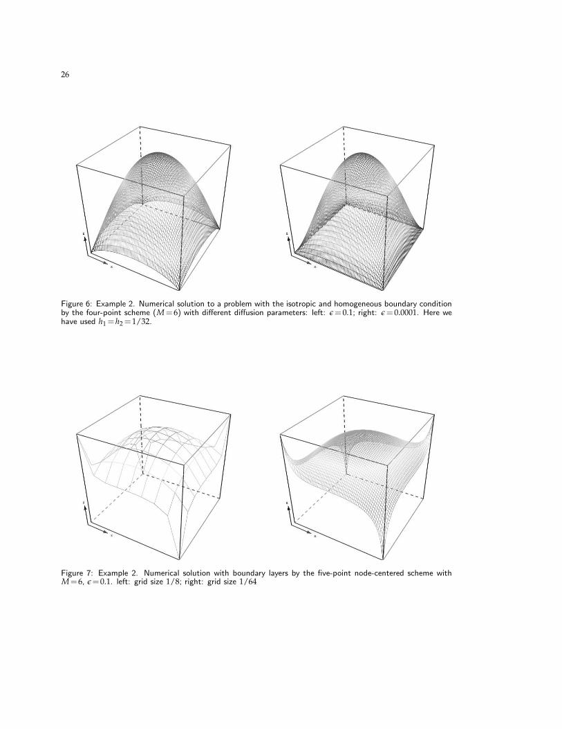
First of all, we check numerically that the diffusion limit can be captured by using isotropicboundary conditions. For different ǫ=0.1 and ǫ=0.0001, the numerical results of usingisotropic boundary conditions ψm|Γ = 0, are presented in Figure 5 and Figure 6. We cansee that even if ǫ is much smaller than the mesh size, the solution of the diffusion limitequation can be captured by TFPS.

Figure 5: Example 2. Numerical solution to a problem with the isotropic and homogeneous boundary conditionby the five-point node-centered scheme (M=6) with different diffusion parameters: left: ǫ=0.1; right: ǫ=0.0001.

When the injected particle densities are anisotropic such that

ψm =

0, if cmsm >0,1, if cmsm <0.

We can see from Figure 7 and Figure 9 that boundary layers appear and both TFPS cancapture the layers by coarse mesh. Especially, in Figure 8 and Figure 10, when ǫ becomessmall, the fast change can be seen even if there is only one node in the layer.

Example 3. We show an example that the coefficients vary with space and have dis-continuous at the interfaces. The computational domain Ω is composed of two partsΩ1=[0,0.5]×[0,0.5] and Ω2=[0,0.5]×(0.5,1]∪(0.5,1]×[0,1]. Ω1 is a transport region withǫ at O(1) while Ω2 is a diffusion region with ǫ very small.

On Ω1: σT =1+10(x2+y2), σa =1+10(x2+y2), q=5, ǫ=0.5;On Ω2: σT =11, σa =5, q=0, ǫ=0.001.

The boundary conditions are anisotropic such that

ψm =

0, if cmsm >0,1, if cmsm <0.

26

Figure 6: Example 2. Numerical solution to a problem with the isotropic and homogeneous boundary conditionby the four-point scheme (M=6) with different diffusion parameters: left: ǫ=0.1; right: ǫ=0.0001. Here wehave used h1 =h2 =1/32.

Figure 7: Example 2. Numerical solution with boundary layers by the five-point node-centered scheme withM=6, ǫ=0.1. left: grid size 1/8; right: grid size 1/64

27

Figure 8: Example 2. Numerical solution with boundary layers by the five-point node-centered scheme withM=6: left: ǫ=0.1; right: ǫ=0.001.

Figure 9: Example 2. Numerical solution with boundary layers by the four-point cell-centered scheme withM=6, ǫ=0.1 on different grids: left: grid size 1/4; right: grid size 1/32. Here we have used h1 =h2 =1/32.

28

Figure 10: Numerical solution with boundary layers by the four-point cell-centered scheme with M = 6: left:ǫ=0.1; right: ǫ=0.001.

The numerical results using the quadrature set S4 (M=6) calculated with different meshesare presented in Figure 11. We can see that both boundary and interface layers exist. Fig-ure 12 presents those values at the cross section x=1/4 calculated with different meshes.The fast changes in the layers can be captured quite well by very coarse mesh.

6 Discussion

This paper presents two uniformly convergent numerical schemes for the steady statediscrete ordinates neutron or radiative transport equation. The idea of the five-pointnode-centered TFPS is that, firstly, approximate the coefficients σT, σa and q in the fourcells around each node by constants, and then locally express the solution by a linearcombination of special solutions of the constant coefficient equation, using which to for-mulate a linear system for the unknown variables at the four neighboring nodes. Theidea of the four-point cell-centered TFPS resembles the finite element method, but thebasis functions in each cell are chosen to be the special solutions of constant coefficientequation and we piece together the numerical solution with the neighboring cells by theinterface conditions at the cell edge centers.

Numerical examples show that the five-point scheme has first-order accuracy and thefour-point scheme has second-order accuracy. Both schemes can capture not only thediffusion limit under isotropic boundary conditions when the mean free path tends tozero, but also the boundary layers without resolving the fast changes, for problems withanisotropic boundary conditions. Furthermore, the four-point cell-centered TFPS can beapplied to problems with discontinuous coefficients. We can use coarse meshes to capturethe interface condition of the diffusion limit equation as well as the fast changes in the

29

interface layers.

In this paper, we only present the construction of two TFPS, demonstrate their uniformconvergence and ability to capture the layers numerically. There are several interestingtheoretical questions worth investigating. For example, the characteristic curves in Fig-ure 1 contain a lot of information about the layer structure and may shed some light tounderstand the ray effect [20]. It is quite crucial to choose those eigenvalue pairs on thex and y axes, which relates to the rectangular meshes we use, but the explanation is openand will be our future subject. Furthermore, the extension of the TFPS to three dimen-sional is straight forward and we will extend this method to more general meshes andcollision kernels.

Acknowledgments

The authors would like to thank Prof. G. Bal for his useful suggestions and comments.

References

[1] M. L. Adams, Discontinuous finite element transport solutions in thick diffusive problems,Nucl Sci Eng, 137 (2001), 298-333.

[2] F. Anli and S. Gungor, A spectral nodal method for one-group x,y,z-cartesian geometry dis-crete ordinates problems, Annals of Nuclear Energy, 23 (1996), 669-680.

[3] Y. Y. Azmy, Arbitrarily high order characteristic methods for solving the neutron transportequation, Ann Nucl Energy. 19 (1992) , 593-606.

[4] G. Bal and L.Ryzhik, Diffusion Approximation of Radiative Transfer Problems with Inter-faces, SIAM, J. Appl. Math., 60(6) (2000),1887-1912.

[5] R.C. De Barros and E.W. Larsen, A numerical method for one-group slab-geometry discreteordinates problems with no spatial truncation error, Nuclear Science and Engineering, 104(1990), 199–208.

[6] R.C. De Barros and E.W. Larsen, A spectral nodal method for one-group x,y-geometry dis-crete ordinates problems, Nuclear Science and Engineering, 111 (1992), 34–45.

[7] C. R. Brennan, R. L. Miller, K. A. Mathews, Split-cell exponential characteristic transportmethod for unstructured tetrahedral meshes, Nucl Sci Eng., 138 (2001), 26-44.

[8] S. Jin, Asymptotic preserving (ap) schemes for multiscale kinetic and hyperbolic equations: areview. lecture notes for summer school on ”methods and models of kinetic theory” (mmkt),tech. report, Rivista di Mathematica della Universita di Parma, Porto Ercole (Grosseto, Italy),2010.

[9] S. Jin, M. Tang and H. Han, A uniformly second order numerical method for the one-dimensional discrete-ordinate transport equation and its diffusion limit with interface, Net-works and Heterogeneous Media, 4, (2009), 35-65.

[10] S. Jin, X. Yang and G. W. Yuan, A domain decomposition method for a two-scale transportequation with energy flux conserved at the interface, Kinetic and Related Models, 1, (2008),65-84.

[11] Houde Han and Zhongyi Huang, A tailored finite point method for the helmholtz equationwith high wave numbers in heterogeneous medium, J. Comp. Math., 26 (2008), 728-739.

30

[12] Houde Han and Zhongyi Huang, Tailored finite point method for a singular perturbationproblem with variable coefficients in two dimensions, Journal of Scientific Computing, 41(2009), 200-220.

[13] Houde Han and Zhongyi Huang, Tailored finite point method for steady-state reaction-diffusion equations, Commun. Math. Sci., 8 (2010), 887-899.

[14] Houde Han, Zhongyi Huang, and R. Bruce Kellogg, The tailored finite point method and aproblem of P. Hemker, in Proceedings of International Conference on Boundary and InteriorLayers – Computational and Asymptotic Methods, 2008.

[15] Houde Han, Zhongyi Huang, and R. Bruce Kellogg, A tailored finite point method for asingular perturbation problem on an unbounded domain, Journal of Scientific Computing,36 (2008), 243–261.

[16] Z. Huang and X. Yang, Tailored finite cell method for solving Helmholtz equation in layeredheterogeneous medium, J Comput. Math.,30(4), (2012),381-391.

[17] E. W. Larsen, J. E. Morel, and W. F. Miller Jr., Asymptotic solutions of numerical transportproblems in optically thick, diffusive regimes, J. Comput. Phys., 69 (1987), 283–324.

[18] E. W. Larsen and J. E. Morel, Asymptotic solutions of numerical transport problems in opti-cally thick,diffusive regimes ii, J. Comput. Phys., 83 (1989), 212–236.

[19] E. W. Larsen, The asymptotic diffusion limit of discretized transport problems. Nucl SciEng., 112 (1992), 336-346, (review)

[20] E. W.Larsen and J. E. Morel, Advances in Discrete-Ordinates Methodology, in Nuclear Com-putational Science: A Century in Review, edited by Y. Y. Azmy and E. Sartori, Springer-Verlag, Berlin. (2010).

[21] R. D. Lawrence, Progress in nodal methods for the solution of the neutron diffusion andtransport equations. Prog Nucl Energy, 17, (1986), 271 (review)

[22] E. E. Lewis and W.F. Miller, Jr. Computational Methods of Neutron Transport. John Wileyand Sons, New York, (1984).

[23] M. Lemou and F. Mehats, Micro-macro schemes for kinetic equations including boundarylayers, SIAM J. Sci. Compt. 34(6) (2012), 734-760.

[24] Yintzer Shih, R. Bruce Kellogg, and Yoyo Chang, Characteristic tailored finite pointmethod for convection-dominated convection-diffusion-reaction problems, Journal of Sci-entific Computing, 47 (2011), 198–215.

[25] Yintzer Shih, R. Bruce Kellogg, and Peishan Tsai, A tailored finite point method forconvection-diffusion-reaction problems, Journal of Scientific Computing, 43 (2010), 239-260.

[26] M. Tang, A uniform first order method for the discrete ordinate transport equation withinterfaces in X,Y-geometry. Journal of Computational Mathematics, 27 (2009), 764-786.

[27] J.S. Warsa, T. A. Wareing, J.E. Morel, Fully consistent diffusion synthetic acceleration of lin-ear discontinuous SN transport discretizations on unstructured tetrahedral meshes. Nucl SciEng., 141 (2002), 236-251.

31

a)

0.181030.18103

0.18103

0.18103

0.18

103

0.18103

0.181030.18103

0.326 0.326

0.32

6

0.326

0.3260.326

0.3260.3260.3260.47097 0.47097 0.47097

0.47097

0.47

097

0.47097

0.47

097

0.470970.47097

0.47

097

0.61594

0.615940.61594

0.76

091

0.760910.76091

0.90588

0.90588

0.90588 1.0509

1.0509

1.0509

1.0509

1.05

09

1.1958

1.1958

1.1958

1.19

58

x

y

0 0.1 0.2 0.3 0.4 0.5 0.6 0.7 0.8 0.9 10

0.1

0.2

0.3

0.4

0.5

0.6

0.7

0.8

0.9

1

0 0.1 0.2 0.3 0.4 0.5 0.6 0.7 0.8 0.9 10

0.5

1

0

0.2

0.4

0.6

0.8

1

1.2

1.4

y

x

φ

b)

0.178520.17852

0.17

852

0.17852

0.17852

0.17852

0.17

852

0.17852

0.32

42

0.3242

0.32420.3242

0.3242

0.32

42

0.32420.32420.3242

0.46988 0.46988 0.469880.46988

0.46

988

0.46988

0.46988

0.469880.46988

0.46

988

0.61557

0.615570.61557

0.76

125

0.761250.76125

0.90693

0.90693

0.906931.0526 1.0526

1.05

26

1.0526

1.05

26

1.198

3

1.1983

1.1983

1.1983

x

y

0 0.1 0.2 0.3 0.4 0.5 0.6 0.7 0.8 0.9 10

0.1

0.2

0.3

0.4

0.5

0.6

0.7

0.8

0.9

1

0 0.1 0.2 0.3 0.4 0.5 0.6 0.7 0.8 0.9 10

0.5

1

0

0.2

0.4

0.6

0.8

1

1.2

1.4

y

x

φ

c)

0.178780.17878

0.17

878

0.17878

0.17878

0.17878

0.17

878

0.178780.325040.32504

0.32504

0.32504

0.32

504

0.32504

0.325040.325040.32504

0.47

131

0.47131 0.47131

0.47

131

0.47131

0.47

131

0.47

131

0.47131

0.471310.47131

0.61757

0.617570.61757

0.76

384

0.763840.76384

0.9101

0.9101

0.9101

1.05

64

1.0564

1.05

64

1.0564

1.0564

1.20

26

1.2026

1.2026

1.2026

x

y

0 0.1 0.2 0.3 0.4 0.5 0.6 0.7 0.8 0.9 10

0.1

0.2

0.3

0.4

0.5

0.6

0.7

0.8

0.9

1

0 0.1 0.2 0.3 0.4 0.5 0.6 0.7 0.8 0.9 10

0.5

1

0

0.2

0.4

0.6

0.8

1

1.2

1.4

y

x

φ

Figure 11: Example 3. The numerical results of different meshes. The left column is the contour plot while theright column depicts the values of φ(x,y). a) h1 =h2 =1/8; b) h1 =h2 =1/16; c) h1 =h2=1/64.

32

0 0.1 0.2 0.3 0.4 0.5 0.6 0.7 0.8 0.9 10

0.2

0.4

0.6

0.8

1

1.2

1.4

x

φ

0 0.1 0.2 0.3 0.4 0.5 0.6 0.7 0.8 0.9 10

0.2

0.4

0.6

0.8

1

1.2

1.4

1.6

x

φ

Figure 12: Example 3. The numerical results at the cross section x=1/4 calculated with different meshes. Herewe have used the four point cell centered TFPS with M=6. The stars, circles and solid lines are respectivelythe numerical results of h1 =h2 =1/8, h1 =h2 =1/16 and h1 =h2=1/64. Left: φ; right: ψ6.

Two Uniform Tailored Finite Point Schemes for the Two...

Documents

Transcript of Two Uniform Tailored Finite Point Schemes for the Two...