Two topics:

neutrino flavor transformationfrom compact object mergers

and

reverse engineering

the rare earth peak

Gail McLaughlin

North Carolina State University

Collaborators: Jim Kneller (NC State), Alex Friedland (SLAC), Annie Malkus (University of Wisconsin), Matt Mumpower (LANL),

Albino Perego (Darmstadt), Andrew Steiner (UTK), Rebecca Surman (Notre Dame), Daavid Vaananen (UBC), Nicole Vaash (Notre

Dame), Alexey Vlasenko (NC State), Yonglin Zhu (NC State)

Topic one: neutrino flavor transformation

Why examine neutrino flavor transformation for mergers?

• neutrinos influence nucleosynthesis

• neutrinos can contribute to jet production

• neutrinos could be detected (if lucky!)

• and any other time you want to know the flavor content of the

neutrino field.

Example: neutrinos influence nucleosynthesis

Neutrinos change the ratio of neutrons to protons

νe + n→ p+ e−

νe + p→ n+ e−

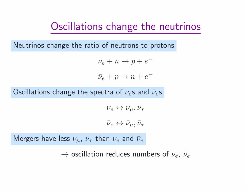
Oscillations change the neutrinos

Neutrinos change the ratio of neutrons to protons

νe + n→ p+ e−

νe + p→ n+ e−

Oscillations change the spectra of νes and νes

νe ↔ νµ, ντ

νe ↔ νµ, ντ

Mergers have less νµ, ντ than νe and νe

→ oscillation reduces numbers of νe, νe

Neutrino oscillations usually studied in free streaming limit

Usually calculated in a regime with few collisions, so above trapping

surfaces → free streaming approximation

Interesting flavor transformation behavior stems from the potentials

neutrinos experience. These potentials come from coherent forward

scattering from neutrons, protons, electrons, positrons, neutrinos.

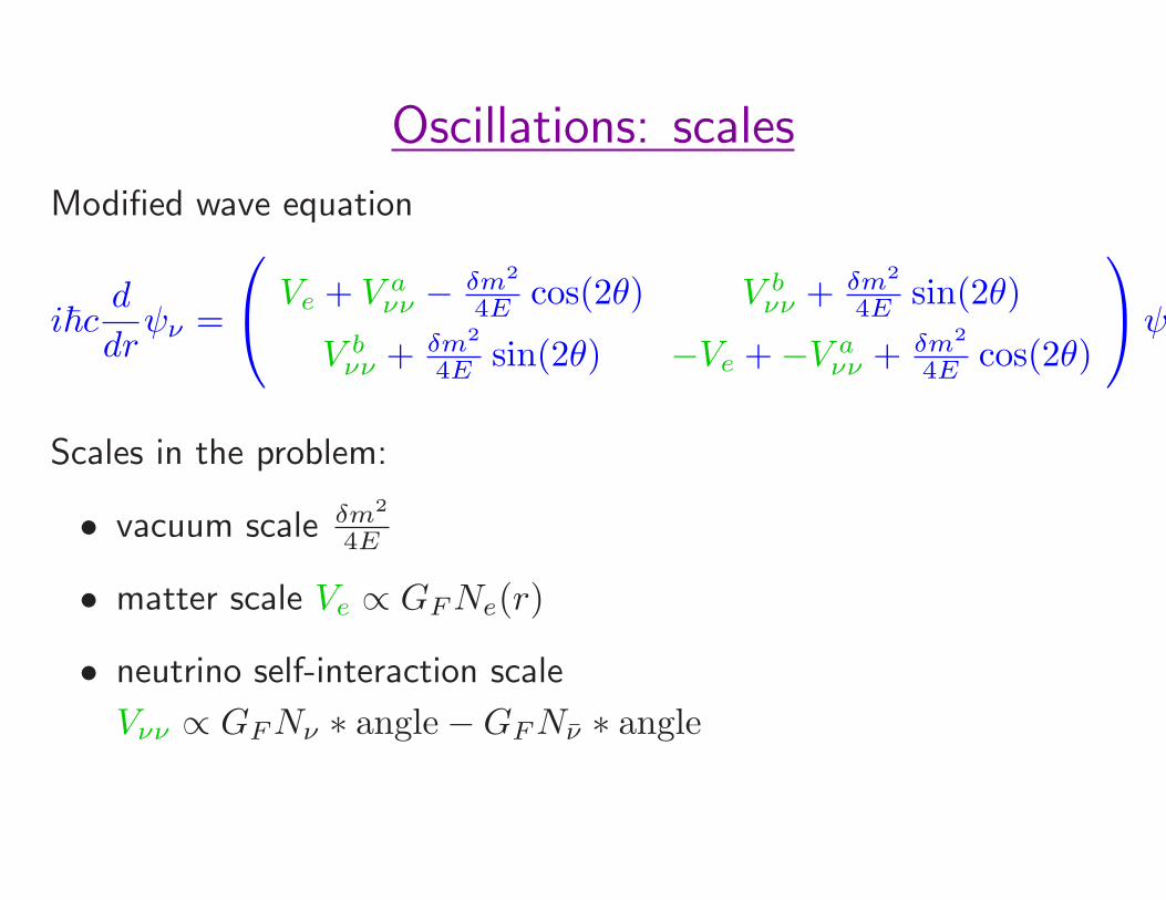
Oscillations: scales

Modified wave equation

i~cd

drψν =

Ve + V aνν − δm2

4E cos(2θ) V bνν + δm2

4E sin(2θ)

V bνν + δm2

4E sin(2θ) −Ve +−V aνν + δm2

4E cos(2θ)

ψ

Scales in the problem:

• vacuum scale δm2

4E

• matter scale Ve ∝ GFNe(r)

• neutrino self-interaction scale

Vνν ∝ GFNν ∗ angle−GFNν ∗ angle

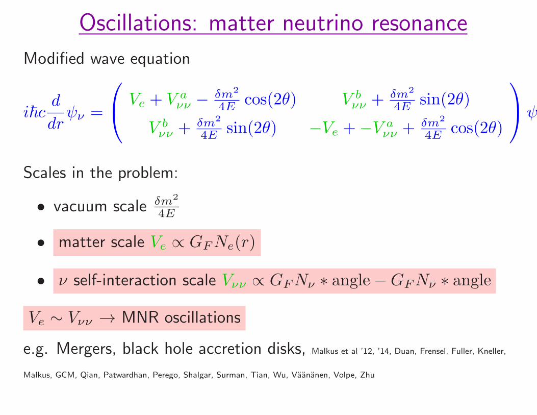
Oscillations: matter neutrino resonance

Modified wave equation

i~cd

drψν =

Ve + V aνν − δm2

4E cos(2θ) V bνν + δm2

4E sin(2θ)

V bνν + δm2

4E sin(2θ) −Ve +−V aνν + δm2

4E cos(2θ)

ψ

Scales in the problem:

• vacuum scale δm2

4E

• matter scale Ve ∝ GFNe(r)

• ν self-interaction scale Vνν ∝ GFNν ∗ angle−GFNν ∗ angle

Ve ∼ Vνν → MNR oscillations

e.g. Mergers, black hole accretion disks, Malkus et al ’12, ’14, Duan, Frensel, Fuller, Kneller,

Malkus, GCM, Qian, Patwardhan, Perego, Shalgar, Surman, Tian, Wu, Vaananen, Volpe, Zhu

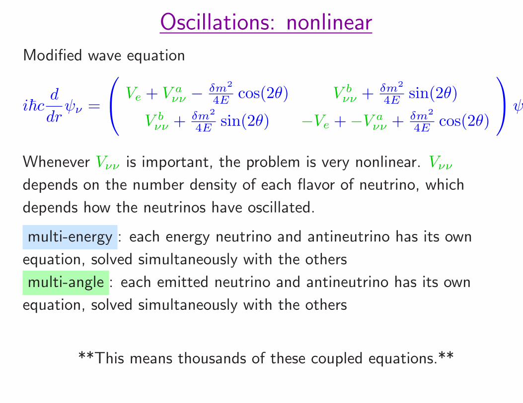
Oscillations: nonlinear

Modified wave equation

i~cd

drψν =

Ve + V aνν − δm2

4E cos(2θ) V bνν + δm2

4E sin(2θ)

V bνν + δm2

4E sin(2θ) −Ve +−V aνν + δm2

4E cos(2θ)

ψ

Whenever Vνν is important, the problem is very nonlinear. Vννdepends on the number density of each flavor of neutrino, which

depends how the neutrinos have oscillated.

multi-energy : each energy neutrino and antineutrino has its own

equation, solved simultaneously with the others

multi-angle : each emitted neutrino and antineutrino has its own

equation, solved simultaneously with the others

**This means thousands of these coupled equations.**

Survival Probabilites

We plot results as survival probabilities.

Pνe= |ψνe

|2, Pνe= |ψνe

|2

Pνeis the probability that a neutrino that starts as electron type will

still be electron type when it is measured later.

Start in flavor states (assume fast oscillations saturate)

Multi-energy, single angle calculation

Neutrino emitting surface is 45 km, T = 6.4 MeV

Antineutrino emitting surface is 45 km, T = 7.1 MeV

Launch a neutrino at 45 degrees.

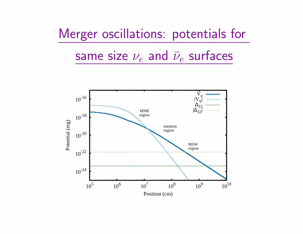
Merger oscillations: potentials for

same size νe and νe surfaces

10-24

10-22

10-20

10-18

10-16

105 106 107 108 109 1010

Pote

ntia

l (er

g)

Position (cm)

MNRregion

nutationregion

MSWregion

Ve|Vν|∆12

|∆32|

Merger oscillations: survival probabilities for

same size νe and νe surfaces

multi-energy, single angle calculations

10-24

10-22

10-20

10-18

10-16

105 106 107 108 109 1010

Pote

ntia

l (er

g)

Position (cm)

MNRregion

nutationregion

MSWregion

Ve|Vν|∆12

|∆32|

fig. from Malkus et al 2016

0 0.2 0.4 0.6 0.8

1 1.2 1.4

Surv

ival

Pro

babi

lity

MNRregion

nutationregion

MSWregion

<P>

<-P>

0 0.2 0.4 0.6 0.8

1 1.2 1.4

105 106 107 108 109 1010

Surv

ival

Pro

babi

lity

Position (cm)

λνe/λνe

0

λ-νe/λ-νe

0

fig. from Malkus et al 2016, see also Frensel et al 2016

MNR transition: explained by single-energy

single-angle model

Compare numerics to prediction Malkus et al, Wu, et al, Vaananen et al

0.2

0.4

0.6

0.8

1Su

rviv

al P

roba

bilit

y

Pνe, num

Pνe, num

Pνe, pred

Pνe, pred

0 5 10 15 20 25 30 35 40

Distance (2E/δm2)

0

500

1000

1500

2000

2500

3000

|V(δ

m2 /2

E)| V

e|Vνν|

Fig. from Malkus et al 2014

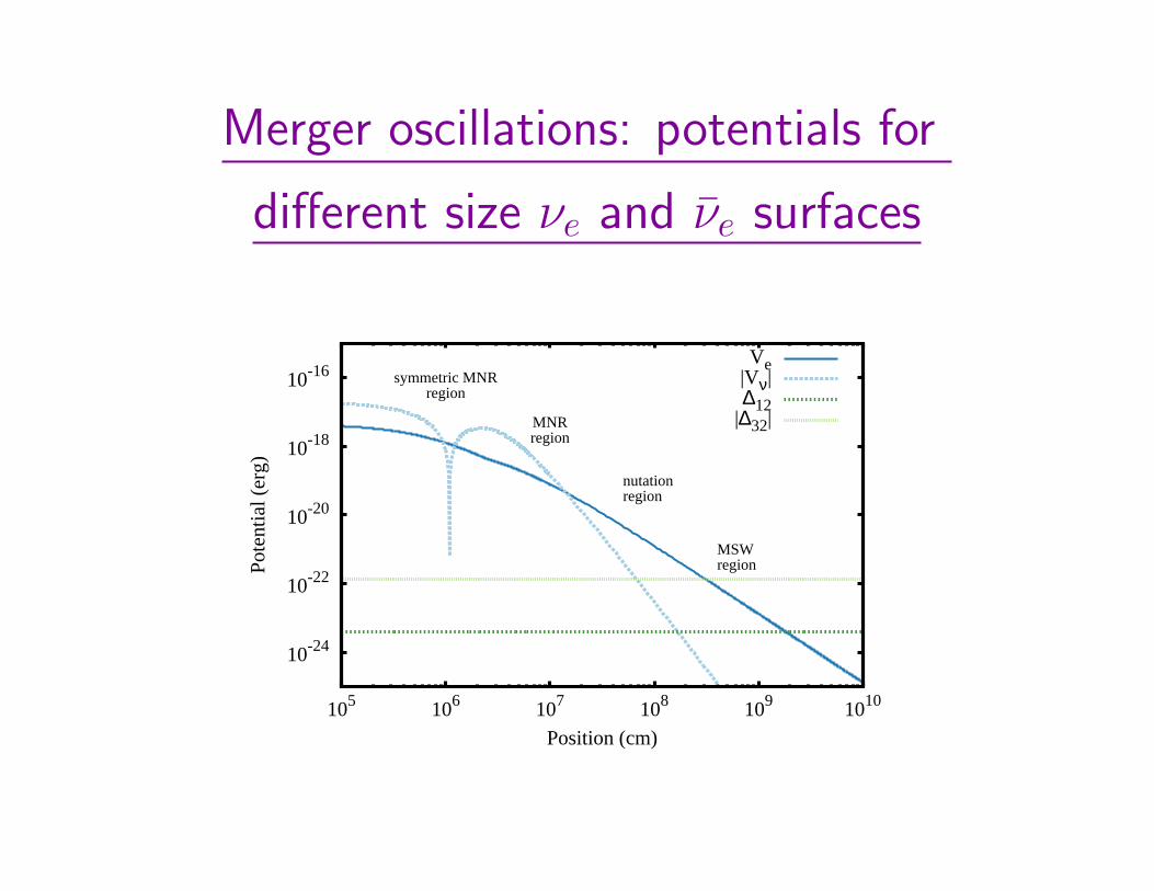
Merger oscillations: potentials for

different size νe and νe surfaces

10-24

10-22

10-20

10-18

10-16

105 106 107 108 109 1010

Pote

ntia

l (er

g)

Position (cm)

symmetric MNRregion

MNRregion

nutationregion

MSWregion

Ve|Vν|∆12

|∆32|

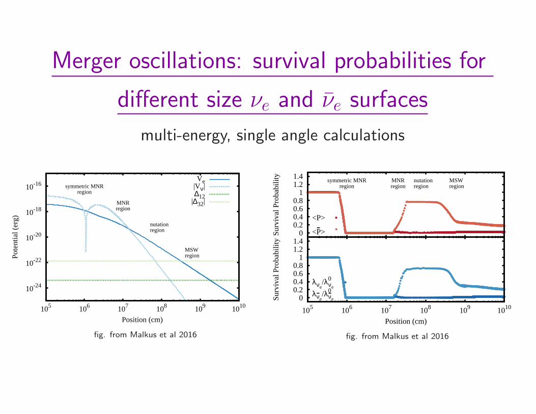
Merger oscillations: survival probabilities for

different size νe and νe surfaces

multi-energy, single angle calculations

10-24

10-22

10-20

10-18

10-16

105 106 107 108 109 1010

Pote

ntia

l (er

g)

Position (cm)

symmetric MNRregion

MNRregion

nutationregion

MSWregion

Ve|Vν|∆12

|∆32|

fig. from Malkus et al 2016

0 0.2 0.4 0.6 0.8

1 1.2 1.4

Surv

ival

Pro

babi

lity

symmetric MNRregion

MNRregion

nutationregion

MSWregion

<P>

<-P>

0 0.2 0.4 0.6 0.8

1 1.2 1.4

105 106 107 108 109 1010

Surv

ival

Pro

babi

lity

Position (cm)

λνe/λνe

0

λ-νe/λ-νe

0

fig. from Malkus et al 2016

Analytic survival probability prediction

also works for symmetric MNR transitions

Geometry causes Vνν to switch sign

Symmetric MNR Fig. from Vaananen ’16

Matter densities in a

dynamical merger calculation

Zhu et al ’16

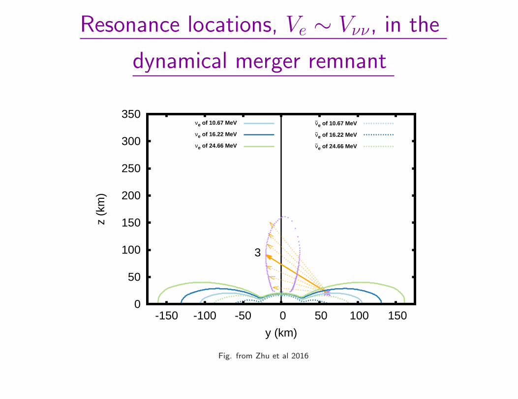
Resonance locations, Ve ∼ Vνν, in the

dynamical merger remnant

0

50

100

150

200

250

300

350

-150 -100 -50 0 50 100 150

z (k

m)

y (km)

3

νe of 10.67 MeV

νe of 16.22 MeV

νe of 24.66 MeV

–νe of 10.67 MeV

–νe of 16.22 MeV

–νe of 24.66 MeV

Fig. from Zhu et al 2016

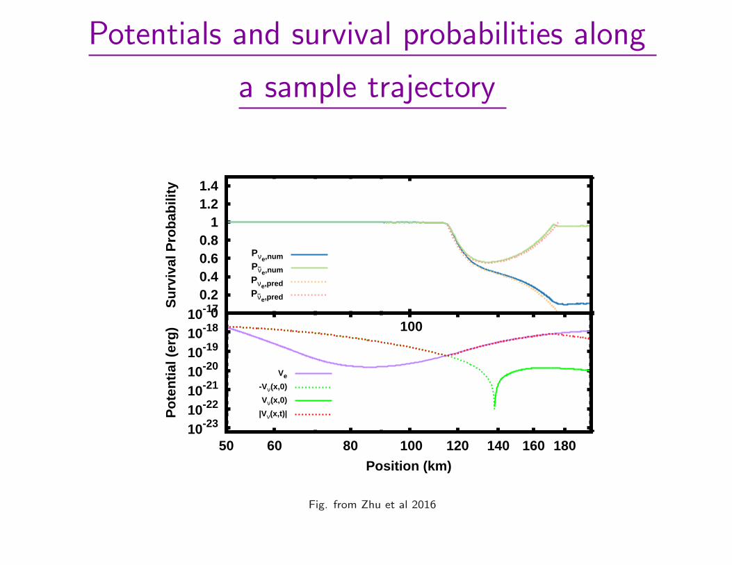
Potentials and survival probabilities along

a sample trajectory

0 0.2 0.4 0.6 0.8

1 1.2 1.4

100

Su

rviv

al P

rob

abili

ty

Pνe,numP–νe,numPνe,predP–νe,pred

10-2310-2210-2110-2010-1910-1810-17

50 60 80 120 140 160 180 100

Po

ten

tial

(er

g)

Position (km)

Ve

-Vν(x,0)

Vν(x,0)

|Vν(x,t)|

Fig. from Zhu et al 2016

Resonance locations, Ve ∼ Vνν, in the

dynamical merger remnant

0

50

100

150

200

250

300

350

-150 -100 -50 0 50 100 150

z (k

m)

y (km)

3

νe of 10.67 MeV

νe of 16.22 MeV

νe of 24.66 MeV

–νe of 10.67 MeV

–νe of 16.22 MeV

–νe of 24.66 MeV

Fig. from Zhu et al 2016

Resonance locations, Ve ∼ Vνν, in the

dynamical merger remnant

0

50

100

150

200

250

300

350

-150 -100 -50 0 50 100 150

z (k

m)

y (km)

12 3 4

νe of 10.67 MeV

νe of 16.22 MeV

νe of 24.66 MeV

–νe of 10.67 MeV

–νe of 16.22 MeV

–νe of 24.66 MeV

Fig. from Zhu et al 2016

Conclusions

Rapid progress in last couple years:

• Predictions of matter neutrino resonance transition behavior

• Likely exists in mergers

• Likely affects nucleosynthesis

What to do next?

• a little more theory work

• keep up with dynamical models as they advance transport

• more physical effects, e.g. general relativity

Long term

• multi-angle effects in full geometry

• decoupling regime, feedback into dynamical calculation

Topic 2:

reverse engineering the

rare earth peak

The solar rare earth peak

Solar abundance data with the rare earth peak in red

Approaches to studying the rare earth peak

Usual procedure:

• Continue to improve hydrodynamics, neutrino transport and

general relativistic treatments in astrophysical simulations

• Calculate abundance pattern with a nuclear model and

thermodynamic conditions as input

Alternative approach:

• Assume a set of thermodynamic conditions

• Back out properties of the nuclear model, for this set of conditions

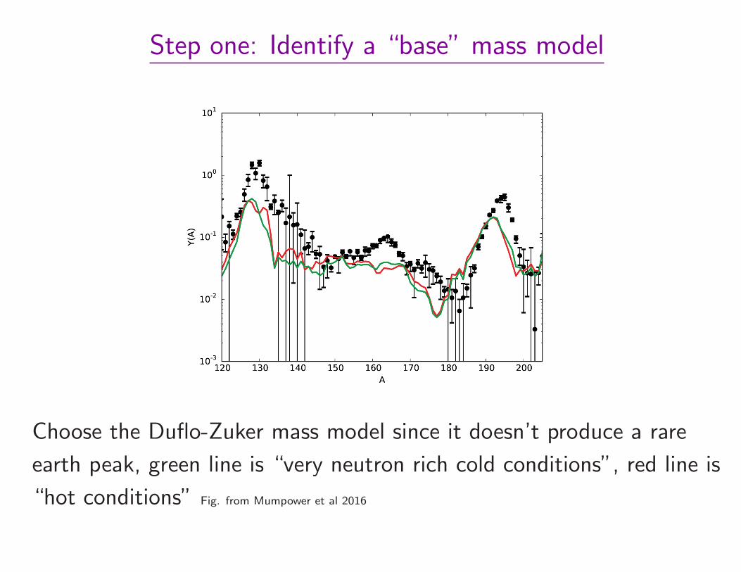
Step one: Identify a “base” mass model

Choose the Duflo-Zuker mass model since it doesn’t produce a rare

earth peak, green line is “very neutron rich cold conditions”, red line is

“hot conditions” Fig. from Mumpower et al 2016

Step two: Add a term to the base model

What term though?

Step two: Add a term to the base model

M(Z,N) =MDZ(Z,N) + aNe−(Z−CZ)2/(2f) (1)

Decision: let each isotone be independent (aN s). Why? Measured

data shows similar isotone structure for nearby elements. Require an

exponential fall off in element number (Z) to avoid altering measured

masses and also to keep the fit to a local region.

Step two: Add a term to the base model

M(Z,N) =MDZ(Z,N) + aNe−(Z−CZ)2/(2f) (2)

Now use MCMC to determine the aN and the CZ

Details: Metropolis algorithm, start with all aN = 0, for each choice of aN , CZ consistent separation energies, beta decay Q

values and neutron capture rates are calculated, algorithm converges in about 10,000 steps.

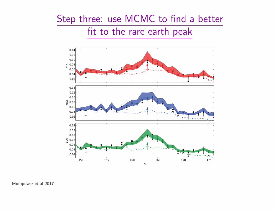
Step three: use MCMC to find a better

fit to the rare earth peak

Mumpower et al 2017

Example calculations

Mumpower et al 2017, Nd isotopic chain

Including measured beta decay rates

Fig. from Nicole Vassh

Comparing with recently measured masses

Fig. from Nicole Vassh

Conclusions

Reverse engineering of nuclear masses looks promising

• use MCMC for nuclear masses, coordinated with neutron capture,

beta decay

• different classes of thermodynamic conditions predict different

mass patterns

Where to go from here

• continue to improve MCMC

• continue compare with (and include) measured data as it becomes

available

• examine additional uncertainties

Conclusions, cont.

Goal

• test the dynamical formation mechansim of the rare earth peak (as

opposed to the fission formation mechanism)

• eventually infer astrophysical conditions, this is complementary to

approach taken by observations, simulations