Two-Sample Test of High Dimensional Means under

Dependency∗

T. Tony Cai, Weidong Liu and Yin Xia

Abstract

This paper considers in the high dimensional setting a canonical testing problem in

multivariate analysis, namely testing the equality of two mean vectors. We introduce

a new test statistic that is based on a linear transformation of the data by the pre-

cision matrix which incorporates the correlations among the variables. Limiting null

distribution of the test statistic and the power of the test are analyzed. It is shown

that the test is particularly powerful against sparse alternatives and enjoys certain

optimality. A simulation study is carried out to examine the numerical performance

of the test and compare with other tests given in the literature. The results show

that the proposed test significantly outperforms those tests in a range of settings.

Keywords: Covariance matrix, extreme value distribution, high dimensional test, hypoth-

esis testing, limiting null distribution, power, precision matrix, testing equality of mean

vectors.

∗Tony Cai is Dorothy Silberberg Professor of Statistics, Department of Statistics, The Wharton School,

University of Pennsylvania, Philadelphia, PA 19104 (Email:tcai@wharton.upenn.edu). The research was

supported in part by NSF FRG Grant DMS-0854973. Weidong Liu is Professor, Department of Math-

ematics, Institute of Natural Sciences and MOE-LSC, Shanghai Jiao Tong University, Shanghai, China

(Email: liuweidong99@gmail.com). Yin Xia is Ph.D student, Department of Statistics, The Wharton

School, University of Pennsylvania, Philadelphia, PA 19104 (Email: xiayin@sas.upenn.edu).

1

1 Introduction

A canonical testing problem in multivariate analysis is that of testing the equality of two

mean vectors µ1 and µ2 based on independent random samples, one from a distribution

with mean µ1 and covariance matrix Σ and another from a distribution with mean µ2 and

the same covariance matrix Σ . This testing problem arises in many scientific applications,

including genetics, econometrics, and signal processing. In the Gaussian setting where one

observes Xk

iid∼ Np(µ1,Σ), k = 1, ..., n1, and Y k

iid∼ Np(µ2,Σ), k = 1, ..., n2, the classical

test for testing the hypotheses

H0 : µ1 = µ2 versus H1 : µ1 = µ2 (1)

is Hotelling’s T 2 test with the test statistic given by

T 2 =n1n2

n1 + n2(X − Y ) Σ

−1(X − Y ),

where X = n−11

n1

k=1 Xk and Y = n−12

n2

k=1 Y k are the sample means and Σ is the

sample covariance matrix. The properties of Hotelling’s T 2 test has been well studied in

the conventional low-dimensional setting. It enjoys desirable properties when the dimension

p is fixed. See, e.g., Anderson (2003).

In many contemporary applications, high dimensional data, whose dimension is often

comparable to or even much larger than the sample size, are commonly available. Examples

include genomics, medical imaging, risk management, and web search problems. In such

high dimensional settings, classical methods designed for the low-dimensional case either

perform poorly or are no longer applicable. For example, the performance of Hotelling’s

T 2 test is unsatisfactory when the dimension is high relative to the sample sizes.

Several proposals for correcting Hotelling’s T 2 statistic have been introduced in the high

dimensional settings. For example, Bai and Saranadasa (1996) proposed to remove Σ−1

in T 2 and introduced a new statistic based on the squared Euclidean norm X − Y 22.

Srivastava and Du (2008) and Srivastava (2009) constructed test statistics by replacing

Σ−1

with the inverse of the diagonal of Σ. Chen and Qin (2010) introduced a test statistic

2

by removing the cross-product terms

n1

i=1 XiX i and

n2

i=1 YiY i in X − Y 22. All of the

above test statistics are based on an estimator of (µ1 − µ2)TA(µ1 − µ2) for some given

positive definite matrix A. We shall call these test statistics sum of squares type statistics

as they all aim to estimate the squared Euclidean norm A12 (µ1 − µ2)22.

It is known that tests based on the sum of squares type statistics can have good power

against the “dense” alternatives. That is, under the alternative hypothesis H1 the signals

in µ1 − µ2 spread out over a large number of coordinates. For a range of applications

including anomaly detection, medical imaging, and genomics, however, the means of the

two populations are typically either identical or are quite similar in the sense that they

only possibly differ in a small number of coordinates. In other words, under the alternative

H1, the difference of the two means µ1 − µ2 is sparse. For example, for ultrasonic flaw

detection in highly-scattering materials, many scattering centers such as grain boundaries

produce echoes and the ensemble of these echoes is usually defined as background noise,

while small cracks, flaws, or other metallurgical defects would be defined as signals. See,

for example, Zhang, Zhang and Wang (2000). In this case, it is natural to take µ1 −µ2 to

be sparse when the metallurgical defects exist. Similarly, for detection of hydrocarbons in

materials, instantaneous spectral analysis is often used to detect hydrocarbons through low-

frequency shadows, which is usually considered as sparse signals. See Castagna, Sun and

Siegfried (2003). In medical imaging, MRI is commonly used for breast cancer detection.

It is used to visualize microcalcifications, which can be an indication of breast cancer. The

signals are rare in such applications, see James, Clymer and Schmalbrock (2001). Another

application is the shape analysis of brain structures, in which the shape differences, if any,

are commonly assumed to be confined to a small number of isolated regions inside the

whole brain. This is equivalent to the sparse alternative. See Cao and Worsley (1999) and

Taylor and Worsley (2008). In these sparse settings, tests based on the sum of squares

type statistics are not powerful. For example, the three tests mentioned earlier all require

(n1+n2)µ1−µ222/p12 → ∞ in order for any of the tests to be able to distinguish between

the null and the alternative with probability tending to 1.

3

The goal of this paper is to develop a test that performs well in general and is particularly

powerful against sparse alternatives in the high dimensional setting under dependency. To

explore the advantages of the dependence between the variables, we introduce a new test

statistic that is based on a linear transformation of the observations by the precision matrix

Ω. Suppose for the moment the precision matrix Ω = Σ−1 is known. For testing the null

hypothesis H0 : µ1 = µ2, we first transform the samples Xk; 1 ≤ k ≤ n1 and Y k; 1 ≤

k ≤ n2 by multiplying with Ω to obtain the transformed samples ΩXk; 1 ≤ k ≤ n1

and ΩY k; 1 ≤ k ≤ n2. The new test statistic is then defined to be the maximum of the

squared two sample t-statistics of the transformed observations ΩXk; 1 ≤ k ≤ n1 and

ΩY k; 1 ≤ k ≤ n2. We shall first show that the limiting null distribution of this test

statistic is the extreme value distribution of type I, and then construct an asymptotically

α level test based on the limiting distribution. It is shown that this test enjoys certain

optimality and uniformly outperforms two other natural tests against sparse alternatives.

The asymptotic properties including the power of the tests are investigated in Section 3.

The covariance matrix Σ and the precision matrix Ω are typically unknown in practice

and thus need to be estimated. Estimation of Σ and Ω in the high dimensional setting

has been well studied in the last few years. See, for example, Yuan and Lin (2007), Bickel

and Levina (2008), Rothman et al. (2008), Ravikumar et al. (2008), Cai, Zhang and Zhou

(2010), Yuan (2010), Cai and Liu (2011), Cai, Liu, and Luo (2011), and Cai and Yuan

(2012). In particular, when Ω is sparse, it can be well estimated by the constrained 1

minimization method proposed in Cai, Liu, and Luo (2011). When such information is

not available, the adaptive thresholding procedure introduced in Cai and Liu (2011) can

be applied to estimate Σ and its inverse is then used to estimate Ω. The estimate of Ω is

then plugged into the test statistic mentioned above to yield a data driven procedure. In

principle, other “good” estimators of Ω can also be used. It is shown that, under regularity

conditions, the data-driven test performs asymptotically as well as the test based on the

oracle statistic and thus shares the same optimality.

A simulation study is carried out to investigate the numerical performance of the pro-

4

posed test in a wide range of settings. The numerical results show that the power of

proposed test uniformly and significantly dominates those of the tests based on the sum of

squares type statistics when either Σ or Ω is sparse. When both Σ and Ω are non-sparse, the

proposed test with the inverse of the adaptive thresholding estimator of Σ still significantly

outperforms the sum of squares type tests.

The rest of the paper is organized as follows. After reviewing basic notation and defini-

tions, Section 2 introduces the new test statistics. Theoretical properties of the proposed

tests are investigated in Section 3. Limiting null distributions of the test statistics and the

power of the tests, both for the case the precision matrix Ω is known and the case Ω is

unknown, are analyzed. Extensions to the non-Gaussian distributions are given in Section

4. A simulation study is carried out in Section 5 to investigate the numerical performance

of the tests. Discussions of the results and other related work are given in Section 6. The

proofs of the main results are delegated in Section 7. Additional simulation results and

theoretical analysis are given in the supplement Cai, Liu and Xia (2013b).

2 Methodology

This section considers the testing problem in the setting of Gaussian distributions. Ex-

tensions to the non-Gaussian case will be discussed in Section 4. We shall first present

our testing procedure in the oracle setting in Section 2.1 where the precision matrix Ω is

assumed to be known. In addition, two other natural testing procedures are introduced

in this setting. A data-driven procedure is given in Section 2.2 for the general case of the

unknown precision matrix Ω by using an estimator of the precision matrix Ω.

We begin with basic notation and definitions. For a vector β = (β1, . . . , βp) ∈ Rp, define

the q norm by |β|q = (

p

i=1 |βi|q)1/q for 1 ≤ q ≤ ∞ with the usual modification for q = ∞.

A vector β is called k-sparse if it has at most k nonzero entries. For a matrix Ω = (ωi,j)p×p,

the matrix 1-norm is the maximum absolute column sum, ΩL1 = max1≤j≤p

p

i=1 |ωi,j|,

the matrix elementwise infinity norm is defined to be |Ω|∞ = max1≤i,j≤p |ωi,j| and the

elementwise 1 norm is Ω1 =

p

i=1

p

j=1 |ωi,j|. For a matrix Ω, we say Ω is k-sparse if

5

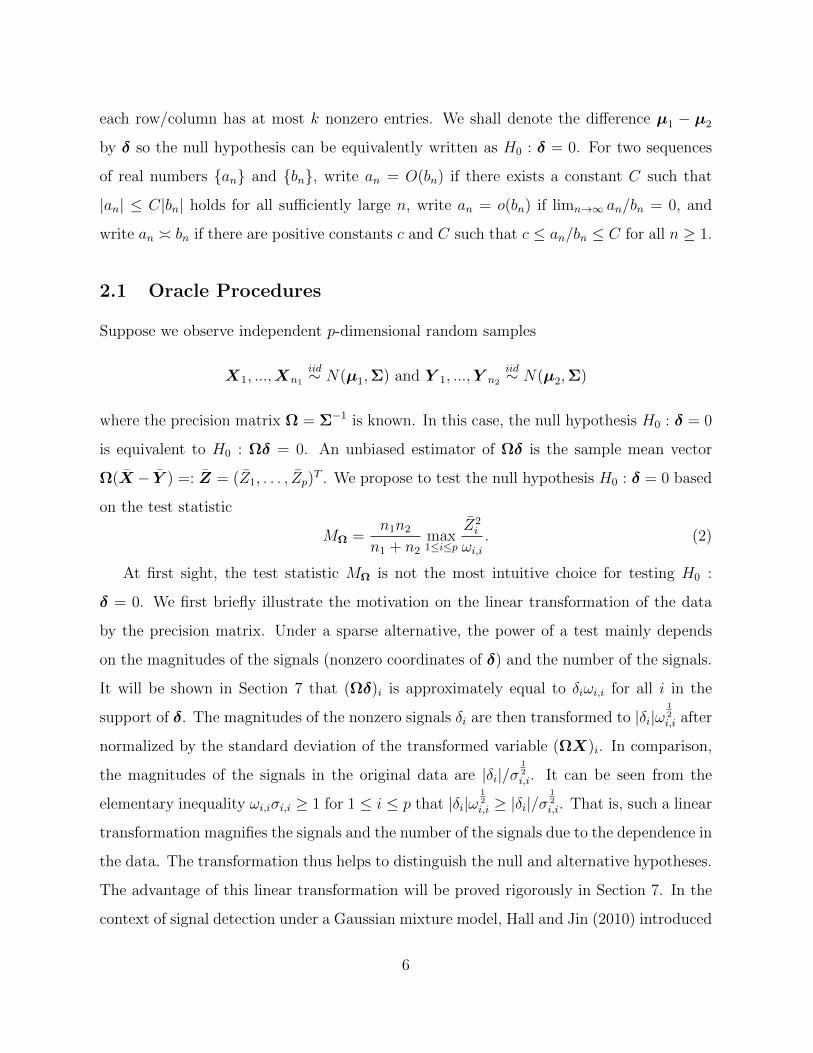
each row/column has at most k nonzero entries. We shall denote the difference µ1 − µ2

by δ so the null hypothesis can be equivalently written as H0 : δ = 0. For two sequences

of real numbers an and bn, write an = O(bn) if there exists a constant C such that

|an| ≤ C|bn| holds for all sufficiently large n, write an = o(bn) if limn→∞ an/bn = 0, and

write an bn if there are positive constants c and C such that c ≤ an/bn ≤ C for all n ≥ 1.

2.1 Oracle Procedures

Suppose we observe independent p-dimensional random samples

X1, ...,Xn1

iid∼ N(µ1,Σ) and Y 1, ...,Y n2

iid∼ N(µ2,Σ)

where the precision matrix Ω = Σ−1 is known. In this case, the null hypothesis H0 : δ = 0

is equivalent to H0 : Ωδ = 0. An unbiased estimator of Ωδ is the sample mean vector

Ω(X − Y ) =: Z = (Z1, . . . , Zp)T . We propose to test the null hypothesis H0 : δ = 0 based

on the test statistic

MΩ =n1n2

n1 + n2max1≤i≤p

Z2i

ωi,i

. (2)

At first sight, the test statistic MΩ is not the most intuitive choice for testing H0 :

δ = 0. We first briefly illustrate the motivation on the linear transformation of the data

by the precision matrix. Under a sparse alternative, the power of a test mainly depends

on the magnitudes of the signals (nonzero coordinates of δ) and the number of the signals.

It will be shown in Section 7 that (Ωδ)i is approximately equal to δiωi,i for all i in the

support of δ. The magnitudes of the nonzero signals δi are then transformed to |δi|ω12i,iafter

normalized by the standard deviation of the transformed variable (ΩX)i. In comparison,

the magnitudes of the signals in the original data are |δi|/σ12i,i. It can be seen from the

elementary inequality ωi,iσi,i ≥ 1 for 1 ≤ i ≤ p that |δi|ω12i,i≥ |δi|/σ

12i,i. That is, such a linear

transformation magnifies the signals and the number of the signals due to the dependence in

the data. The transformation thus helps to distinguish the null and alternative hypotheses.

The advantage of this linear transformation will be proved rigorously in Section 7. In the

context of signal detection under a Gaussian mixture model, Hall and Jin (2010) introduced

6

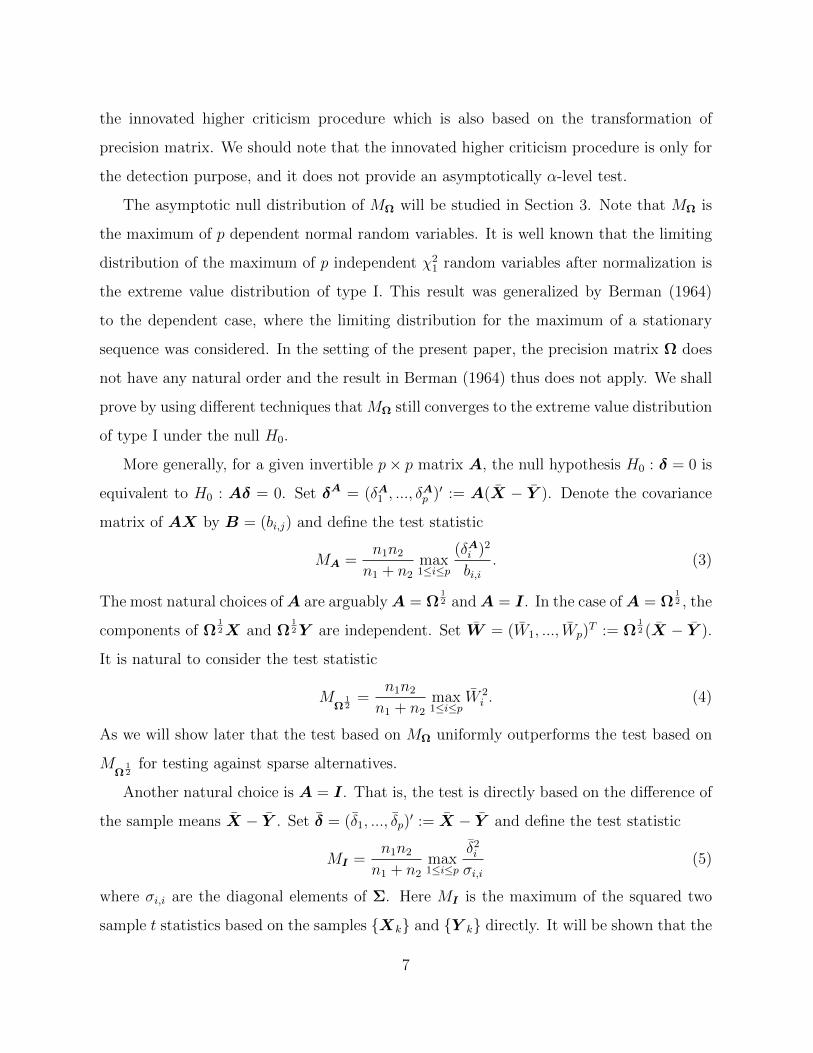
the innovated higher criticism procedure which is also based on the transformation of

precision matrix. We should note that the innovated higher criticism procedure is only for

the detection purpose, and it does not provide an asymptotically α-level test.

The asymptotic null distribution of MΩ will be studied in Section 3. Note that MΩ is

the maximum of p dependent normal random variables. It is well known that the limiting

distribution of the maximum of p independent χ21 random variables after normalization is

the extreme value distribution of type I. This result was generalized by Berman (1964)

to the dependent case, where the limiting distribution for the maximum of a stationary

sequence was considered. In the setting of the present paper, the precision matrix Ω does

not have any natural order and the result in Berman (1964) thus does not apply. We shall

prove by using different techniques thatMΩ still converges to the extreme value distribution

of type I under the null H0.

More generally, for a given invertible p× p matrix A, the null hypothesis H0 : δ = 0 is

equivalent to H0 : Aδ = 0. Set δA = (δA1 , ..., δAp) := A(X − Y ). Denote the covariance

matrix of AX by B = (bi,j) and define the test statistic

MA =n1n2

n1 + n2max1≤i≤p

(δAi)2

bi,i. (3)

The most natural choices ofA are arguablyA = Ω12 andA = I. In the case ofA = Ω

12 , the

components of Ω12X and Ω

12Y are independent. Set W = (W1, ..., Wp)T := Ω

12 (X − Y ).

It is natural to consider the test statistic

MΩ

12=

n1n2

n1 + n2max1≤i≤p

W 2i. (4)

As we will show later that the test based on MΩ uniformly outperforms the test based on

MΩ

12for testing against sparse alternatives.

Another natural choice is A = I. That is, the test is directly based on the difference of

the sample means X − Y . Set δ = (δ1, ..., δp) := X − Y and define the test statistic

MI =n1n2

n1 + n2max1≤i≤p

δ2i

σi,i

(5)

where σi,i are the diagonal elements of Σ. Here MI is the maximum of the squared two

sample t statistics based on the samples Xk and Y k directly. It will be shown that the

7

test based on MI is uniformly outperformed by the test based on MΩ for testing against

sparse alternatives.

2.2 Data-Driven Procedure

We have so far focused on the oracle case in which the precision matrix Ω is known.

However, in most applications Ω is unknown and thus needs to be estimated. We consider

in this paper two procedures for estimating the precision matrix. When Ω is known to be

sparse, the CLIME estimator proposed in Cai, Liu and Luo (2011) is used to estimate Ω

directly. If such information is not available, we first estimate the covariance matrix Σ by

the inverse of the adaptive thresholding estimator Σ

introduced in Cai and Liu (2011),

and then estimate Ω by (Σ

)−1.

We first consider the CLIME estimator. Let Σn be the pooled sample covariance matrix

(σi,j)p×p = Σn =1

n1 + n2

n1

k=1

(Xk − X)(Xk − X)+

n2

k=1

(Y k − Y )(Y k − Y ).

Let Ω1 = (ω1i,j) be a solution of the following optimization problem:

min Ω1 subject to |ΣnΩ− I|∞ ≤ λn,

where · 1 is the elementwise 1 norm, and λn = Clog p/n for some sufficiently large

constant C. In practice, λn can be chosen through cross validation. See Cai, Liu, and

Luo (2011) for further details. The estimator of the precision matrix Ω is defined to be

Ω = (ωi,j)p×p, where

ωi,j = ωj,i = ω1i,jI|ω1

i,j| ≤ |ω1

j,i|+ ω1

j,iI|ω1

i,j| > |ω1

j,i|.

The estimator Ω is called the CLIME estimator and can be implemented by linear pro-

gramming. It enjoys desirable theoretical and numerical properties. See Cai, Liu, and Luo

(2011) for more details on the properties and implementation of this estimator.

When the precision matrix Ω is not known to be sparse, we estimate Ω by Ω = (Σ

)−1,

the inverse of the adaptive thresholding estimator of Σ. The adaptive thresholding esti-

8

mator Σ

= (σ

i,j)p×p is defined by

σ

i,j= σi,jI(|σi,j| ≥ λi,j)

with λi,j = δ

θi,j log pn

, where

θi,j =1

n1 + n2

n1

k=1

(Xki − X i)(Xkj − Xj)− σi,j

2

+n2

k=1

(Yki − Y i)(Ykj − Y j)− σi,j

2

X i = n−11

n1

k=1

Xki, Y i = n−12

n2

k=1

Yki

is an estimate of θi,j = Var((Xi − µi)(Xj − µj)). Here δ is a tuning parameter which

can be taken as fixed at δ = 2 or can be chosen empirically through cross-validation. This

estimator is easy to implement and it enjoys desirable theoretical and numerical properties.

See Cai and Liu (2011) for more details on the properties of this estimator.

For testing the hypothesis H0 : µ1 = µ2 in the case of unknown precision matrix Ω,

motivated by the oracle procedure MΩ given in Section 2.1, our final test statistic is MΩ

defined by

MΩ =n1n2

n1 + n2max1≤i≤p

Z2i

ω(0)i,i

, (6)

where Z = ( Z1, . . . , Zp)T := Ω(X − Y ) and ω(0)i,i

= n1n1+n2

ω(1)i,i

+ n2n1+n2

ω(2)i,i

with

(ω(1)i,j) :=

1

n1

n1

k=1

(ΩXk − X Ω)(ΩXk − X Ω)

T ,

(ω(2)i,j) :=

1

n2

n2

k=1

(ΩY k − Y Ω)(ΩY k − Y Ω)

T ,

X Ω = n−11

n1

k=1

ΩXk, Y Ω = n−12

n2

k=1

ΩY k. (7)

It will be shown in Section 3 that MΩ and MΩ have the same asymptotic null distribution

and power under certain regularity conditions. Note that other estimators of the precision

matrix Ω can also be used to construct a good test. See more discussions in Section 3.2.2.

9

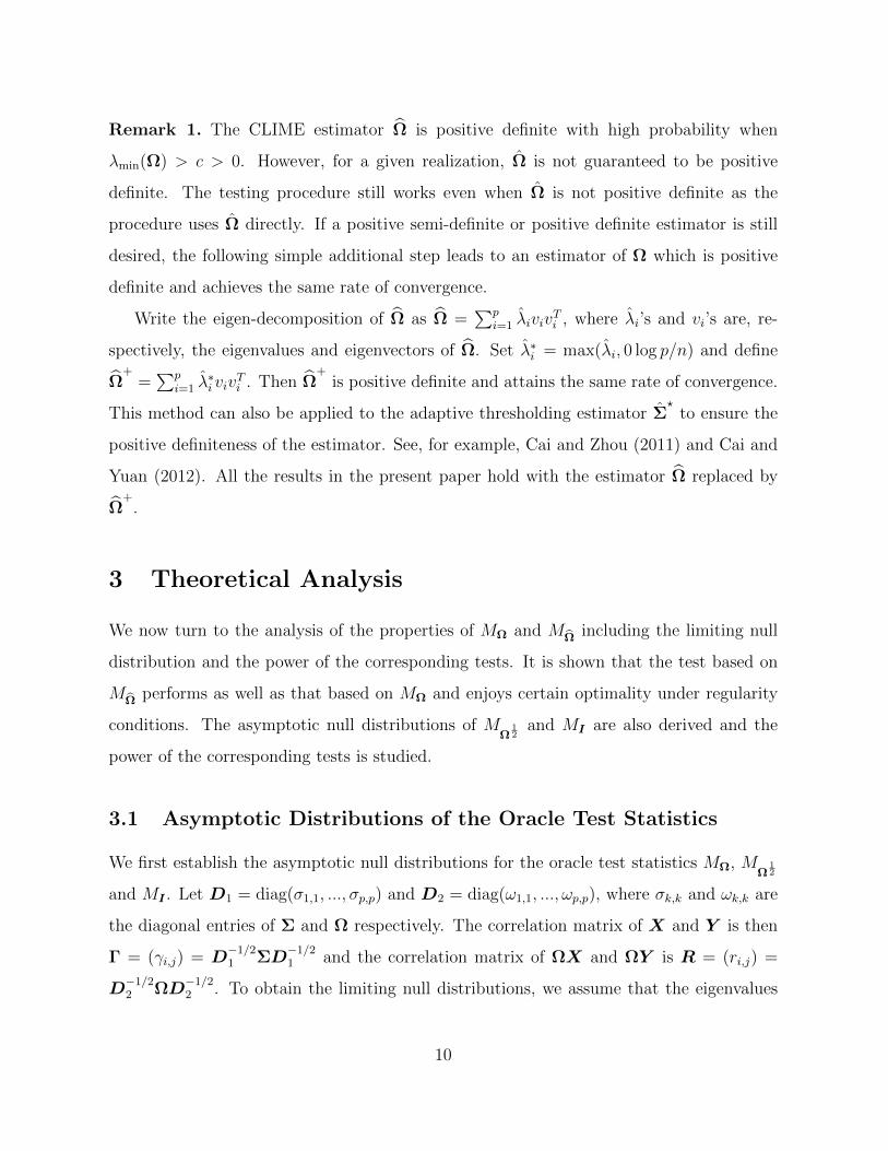
Remark 1. The CLIME estimator Ω is positive definite with high probability when

λmin(Ω) > c > 0. However, for a given realization, Ω is not guaranteed to be positive

definite. The testing procedure still works even when Ω is not positive definite as the

procedure uses Ω directly. If a positive semi-definite or positive definite estimator is still

desired, the following simple additional step leads to an estimator of Ω which is positive

definite and achieves the same rate of convergence.

Write the eigen-decomposition of Ω as Ω =

p

i=1 λivivTi , where λi’s and vi’s are, re-

spectively, the eigenvalues and eigenvectors of Ω. Set λ∗i= max(λi, 0 log p/n) and define

Ω+=

p

i=1 λ∗ivivTi . Then Ω

+is positive definite and attains the same rate of convergence.

This method can also be applied to the adaptive thresholding estimator Σ

to ensure the

positive definiteness of the estimator. See, for example, Cai and Zhou (2011) and Cai and

Yuan (2012). All the results in the present paper hold with the estimator Ω replaced by

Ω+.

3 Theoretical Analysis

We now turn to the analysis of the properties of MΩ and MΩ including the limiting null

distribution and the power of the corresponding tests. It is shown that the test based on

MΩ performs as well as that based on MΩ and enjoys certain optimality under regularity

conditions. The asymptotic null distributions of MΩ

12and MI are also derived and the

power of the corresponding tests is studied.

3.1 Asymptotic Distributions of the Oracle Test Statistics

We first establish the asymptotic null distributions for the oracle test statistics MΩ, MΩ12

and MI . Let D1 = diag(σ1,1, ..., σp,p) and D2 = diag(ω1,1, ...,ωp,p), where σk,k and ωk,k are

the diagonal entries of Σ and Ω respectively. The correlation matrix of X and Y is then

Γ = (γi,j) = D−1/21 ΣD−1/2

1 and the correlation matrix of ΩX and ΩY is R = (ri,j) =

D−1/22 ΩD−1/2

2 . To obtain the limiting null distributions, we assume that the eigenvalues

10

of the covariance matrix Σ are bounded from above and below, and the correlations in Γ

and R are bounded away from −1 and 1. More specifically we assume the following:

(C1): C−10 ≤ λmin(Σ) ≤ λmax(Σ) ≤ C0 for some constant C0 > 0;

(C2): max1≤i<j≤p |γi,j| ≤ r1 < 1 for some constant 0 < r1 < 1;

(C3): max1≤i<j≤p |ri,j| ≤ r2 < 1 for some constant 0 < r2 < 1.

Condition (C1) on the eigenvalues is a common assumption in the high-dimensional

setting. Conditions (C2) and (C3) are also mild. For example, if max1≤i<j≤p |ri,j| = 1, then

Σ is singular. The following theorem states the asymptotic null distributions for the three

oracle statistics MΩ, MΩ12and MI .

Theorem 1. Let the test statistics MΩ, MΩ12and MI be defined as in (2), (4) and (5),

respectively.

(i). Suppose that (C1) and (C3) hold. Then for any x ∈ R,

PH0

MΩ − 2 log p+ log log p ≤ x

→ exp

− 1√

πexp(−x

2), as p → ∞.

(ii). For any x ∈ R,

PH0

M

Ω12− 2 log p+ log log p ≤ x

→ exp

− 1√

πexp(−x

2), as p → ∞.

(iii). Suppose that (C1) and (C2) hold. Then for any x ∈ R,

PH0

MI − 2 log p+ log log p ≤ x

→ exp

− 1√

πexp(−x

2), as p → ∞.

Theorem 1 holds for any fixed sample sizes n1 and n2 and it shows that MΩ, MΩ12and

MI have the same asymptotic null distribution. Based on the limiting null distribution,

three asymptotically α-level tests can be defined as follows:

Φα(Ω) = IMΩ ≥ 2 log p− log log p+ qα,

Φα(Ω12 ) = IM

Ω12≥ 2 log p− log log p+ qα,

Φα(I) = IMI ≥ 2 log p− log log p+ qα,

11

where qα is the 1−α quantile of the type I extreme value distribution with the cumulative

distribution function exp− 1√

πexp(−x/2)

, i.e.,

qα = − log(π)− 2 log log(1− α)−1.

The null hypothesis H0 is rejected if and only if Φα(·) = 1. Although the asymptotic

null distribution of the test statistics MΩ, MI , and MΩ

12are the same, the power of the

tests Φα(Ω), Φα(Ω12 ), and Φα(I) are quite different. We shall show in Section 1 in the

supplementary material Cai, Liu and Xia (2013b) that the power of Φα(Ω) uniformly

dominates those of Φα(Ω12 ) and Φα(I) when testing against sparse alternatives, and the

results are briefly summarized in Section 3.2.3.

3.2 Asymptotic Properties of Φα(Ω) And Φα(Ω)

In this section, the asymptotic power of MΩ is analyzed and the test Φα(Ω) is shown to

be minimax rate optimal. In practice, Ω is unknown and the test statistic MΩ should be

used instead of MΩ. Define the set of kp-sparse vectors by

S(kp) =δ :

p

j=1

Iδj = 0 = kp.

Throughout the section, we analyze the power of MΩ and MΩ under the alternative

H1 : δ ∈ S(kp) with kp = pr, 0 ≤ r < 1, and the nonzero

locations are randomly uniformly drawn from 1, ..., p,

Under H1, we let (X − µ1,Y − µ2) be independent with the nonzero locations of δ. As

discussed in the introduction, the condition on the nonzero coordinates in H1 is mild.

Similar conditions have been imposed in Hall and Jin (2008), Hall and Jin (2010) and

Arias-Castro, Candes and Plan (2011). We show that, under certain sparsity assumptions

on Ω, MΩ performs as well as MΩ asymptotically. For the following sections, we assume

n1 n2 and write n = n1n2n1+n2

.

12

3.2.1 Asymptotic Power And Optimality of Φα(Ω)

The asymptotic power of Φα(Ω) is analyzed under certain conditions on the separation

between µ1 and µ2. Furthermore, a lower bound is derived to show that this condition is

minimax rate optimal in order to distinguish H1 and H0 with probability tending to 1.

Theorem 2. Suppose (C1) holds. Under the alternative H1 with r < 1/4, if maxi |δi/σ12i,i| ≥

2β log p/n with β ≥ 1/(mini σi,iωi,i) + ε for some constant ε > 0, then as p → ∞

PH1

Φα(Ω) = 1

→ 1.

We shall show that the condition maxi |δi/σ12i,i| ≥

2β log p/n is minimax rate optimal

for testing against sparse alternatives. First we introduce some conditions.

(C4) kp = pr for some r < 1/2 and Ω = Σ−1 is sp-sparse with sp = O((p/k2

p)γ) for some

0 < γ < 1.

(C4) kp = pr for some r < 1/4.

(C5) ΩL1 ≤ M for some constant M > 0.

Define the class of α-level tests by

Tα = Φα : PH0

Φα = 1

≤ α.

The following theorem shows that the condition maxi |δi/σ12i,i| ≥

2β log p/n is minimax

rate optimal.

Theorem 3. Assume that (C4) (or (C4)) and (C5) hold. Let α, ν > 0 and α + ν < 1.

Then there exists a positive constant c such that for all sufficiently large n and p,

infδ∈S(kp)∩|δ|∞≥c

√log p/n

supΦα∈Tα

P(Φα = 1) ≤ 1− ν.

Theorem 3 shows that, if c is sufficiently small, then any α level test is unable to

reject the null hypothesis correctly uniformly over δ ∈ S(kp) ∩ |δ|∞ ≥ c

log p/n with

probability tending to one. So the order of the lower bound maxi |δi/σ12i,i| ≥

2β log p/n

can not be improved.

13

3.2.2 Asymptotic Properties And Optimality of Φα(Ω)

We now analyze the properties of MΩ and the corresponding test including the limiting

null distribution and the asymptotic power. We shall assume the estimator Ω = (ωi,j) has

at least a logarithmic rate of convergence

Ω−ΩL1 = oP(1

log p) and max

1≤i≤p

|ωi,i − ωi,i| = oP(1

log p). (8)

This is a rather weak requirement on Ω and, as will be shown later, can be easily satisfied

by the CLIME estimator or the inverse of the adaptive thresholding estimator for a wide

range of covariance/precision matrices. We will show that under Condition (8) MΩ has the

same limiting null distribution as MΩ. Define the corresponding test Φα(Ω) by

Φα(Ω) = IMΩ ≥ 2 log p− log log p+ qα.

The following theorem show that MΩ and MΩ have the same asymptotic distribution and

power under Condition (8), and so the test Φα(Ω) is also minimax rate optimal.

Theorem 4. Suppose that Ω satisfies (8) and (C1) and (C3) hold.

(i). Then under the null hypothesis H0, for any x ∈ R,

PH0

MΩ − 2 log p+ log log p ≤ x

→ exp

− 1√

πexp(−x

2), as n, p → ∞.

(ii). Under the alternative hypothesis H1 with r < 1/6, we have, as n, p → ∞,

PH1

Φα(Ω) = 1

PH1

Φα(Ω) = 1

→ 1.

Furthermore, if maxi |δi/σ12i,i| ≥

2β log p/n with β ≥ 1/(mini σi,iωi,i) + ε for some

constant ε > 0, then

PH1

Φα(Ω) = 1

→ 1, as n, p → ∞.

14

As mentioned earlier, Condition (8) is rather weak and is satisfied by the CLIME

estimator or the inverse of the adaptive thresholding estimator for a wide range of pre-

cision/covariance matrices. It is helpful to give a few examples of collections of preci-

sion/covariance matrices for which (8) holds.

We first consider the following class of precision matrices that satisfy an q-ball con-

straint for each row/column. Let 0 ≤ q < 1 and define

Uq(sp,1,Mp) =Ω 0 : ΩL1 ≤ Mp, max

1≤j≤p

p

i=1

|ωi,j|q ≤ sp,1. (9)

The class Uq(sp,1,Mp) covers a range of precision matrices as the parameters q, sp,1 and Mp

vary. Using the techniques in Cai, Liu and Luo (2011), Proposition 1 below shows that (8)

holds for the CLIME estimator if Ω ∈ Uq(sp,Mp) with

sp,1 = o n(1−q)/2

M1−q

p (log p)(3−q)/2

. (10)

We now turn to the covariance matrices. Consider a large class of covariance matrices

defined by, for 0 ≤ q < 1,

U

q(sp,2,Mp) =

Σ : Σ 0, Σ−1L1 ≤ Mp, max

i

p

j=1

(σi,iσj,j)(1−q)/2|σi,j|q ≤ sp,2

. (11)

Matrices in U

q(sp,2) satisfy a weighted q-ball constraint for each row/column. Let Ω =

(Σ

)−1, where Σ

is the adaptive thresholding estimator defined in Section 2.2. Then

Proposition 1 below shows that Condition (8) is satisfied by Ω if Σ ∈ U

q(sp,2,Mp) with

sp,2 = o n(1−q)/2

M2p(log p)(3−q)/2

. (12)

Besides the class of covariance matrices U

q(sp,2,Mp) given in (11), Condition (8) is also

satisfied by the inverse of the adaptive thresholding estimator Ω = (Σ

)−1 over the class

of bandable covariance matrices defined by

Fα(M1,M2) =

Σ : Σ 0, Σ−1L1 ≤ M1, maxj

i:|i−j|>k

|σi,j| ≤ M2k−α, for k ≥ 1

where α > 0, M1 > 0 and M2 > 0. This class of covariance matrices arises naturally in

time series analysis. See Cai, Zhang and Zhou (2010) and Cai and Zhou (2012).

15

Proposition 1. Suppose that log p = o(n1/3) and (C1) holds. Then the CLIME estimator

for Ω ∈ Uq(sp,1,Mp) with (10) satisfies (8). Similarly, the inverse of the adaptive threshold-

ing estimator of Σ ∈ U

q(sp,2,Mp) with (12) or Σ ∈ Fα(M1,M2) with log p = o(nα/(4+3α))

satisfies (8).

We should note that the conditions (8) , (10), and (12) are technical conditions and

they can be further weakened. For example, the following result holds without imposing a

sparsity condition on Ω.

Theorem 5. Let Ω be the CLIME estimator. Suppose that (C1) and (C3) hold and

mini ωi,i ≥ c for some c > 0. If ΩL1 ≤ Mp and

M2p= o(

√n/(log p)3/2), (13)

then

PH0(Φα(Ω) = 1) ≤ α + o(1), as n, p → ∞.

Furthermore, if maxi |δi/σ12i,i| ≥

2β log p/n with β ≥ 1/(mini σi,iωi,i)+ε for some constant

ε > 0, then

PH1(Φα(Ω) = 1) → 1, as n, p → ∞.

3.2.3 Power Comparison of the Oracle Tests

The tests Φα(Ω) and Φα(Ω) are shown in Sections 3.2.1 and 3.2.2 to be minimax rate

optimal for testing against sparse alternatives. Under some additional regularity conditions,

it can be shown that the test Φα(Ω) is uniformly at least as powerful as both Φα(Ω12 ) and

Φα(I), and the results are stated in Proposition 1 in the supplementary material Cai, Liu

and Xia (2013b). Furthermore, we show that, for a class of alternatives, the test Φα(Ω) is

strictly more powerful than both Φα(Ω12 ) and Φα(I). For further details, see Propositions

2 and 3 in the supplementary material Cai, Liu and Xia (2013b). On the other hand, we

should also note that the relative performance of the three oracle tests, Φα(Ω), Φα(Ω12 ),

and Φα(I), is not clear in the non-sparse case. It is possible, for example, when kp = pr

for some r > 1/2, Φα(Ω) might be outperformed by Φα(Ω12 ) or Φα(I).

16

4 Extension to Non-Gaussian Distributions

We have so far focused on the Gaussian setting and studied the asymptotic null distributions

and power of the tests. In this section, the results for the tests Φα(Ω) and Φα(Ω) are

extended to non-Gaussian distributions.

We require some moment conditions on the distributions of X and Y . Let X and Y

be two p-dimensional random vectors satisfying

X = µ1 +U 1 and Y = µ2 +U 2,

where U 1 and U 2 are independent and identical distributed random vectors with mean zero

and covariance matrix Σ = (σi,j)p×p. Let V j = ΩU j =: (V1j, . . . , Vpj)T for j = 1, 2. The

moment conditions are divided into two cases: the sub-Gaussian-type tails and polynomial-

type tails.

(C6). (Sub-Gaussian-type tails) Suppose that log p = o(n1/4). There exist some

constants η > 0 and K > 0 such that

E exp(ηV 2i1/ωi,i) ≤ K and E exp(ηV 2

i2/ωi,i) ≤ K for 1 ≤ i ≤ p.

(C7). (Polynomial-type tails) Suppose that for some constants γ0, c1 > 0, p ≤ c1nγ0 ,

and for some constants > 0 and K > 0

E|Vi1/ω12i,i|2γ0+2+ ≤ K and E|Vi2/ω

12i,i|2γ0+2+ ≤ K for 1 ≤ i ≤ p.

Theorem 6. Suppose that (C1), (C3) and (C6) (or (C7)) hold. Then under the null

hypothesis H0, for any x ∈ R,

PH0

MΩ − 2 log p+ log log p ≤ x

→ exp

− 1√

πexp(−x

2), as n, p → ∞.

Theorem 6 shows that Φα(Ω) is still an asymptotically α-level test when the distribution

is non-Gaussian. When Ω is unknown, as in the Gaussian case, the CLIME estimator Ω

in Cai, Liu and Luo (2011) or the inverse of adaptive thresholding estimator (Σ

)−1 can

be used. The following theorem shows that the test Φα(Ω) shares the same optimality as

Φα(Ω) in the non-Gaussian setting.

17

Theorem 7. Suppose that (C1), (C3), (C6) (or (C7)) and (8) hold.

(i). Under the null hypothesis H0, for any x ∈ R,

PH0

MΩ − 2 log p+ log log p ≤ x

→ exp

− 1√

πexp(−x

2), as n, p → ∞.

(ii). Under H1 and the conditions of Theorem 2, we have

PH1

Φα(Ω) = 1

→ 1, as n, p → ∞.

5 Simulation Study

In this section, we consider the numerical performance of the proposed test Φα(Ω) and

compare it with a number of other tests, including the tests based on the sum of squares

type statistics in Bai and Saranadasa (1996), Srivastava and Du (2009), Chen and Qin

(2010), and the commonly used Hotelling’s T 2 test. These last four tests are denoted

respectively by BS, SD, CQ and T 2 respectively in the rest of this section.

The test Φα(Ω) is easy to implement. A range of covariance structures are considered

in the simulation study, including the settings where the covariance matrix Σ is sparse,

the precision matrix Ω is sparse, and both Σ and Ω are non-sparse. In the case when Ω is

known to be sparse, the CLIME estimator in Cai, Liu and Luo (2011) is used to estimate

it, while the inverse of the adaptive thresholding estimator in Cai and Liu (2011) is used

to estimate Ω when such information is not available. The simulation results show that

the test Φα(Ω) significantly and uniformly outperforms the other four tests when either Σ

or Ω is sparse, and the test Φα(Ω) still outperforms the other four tests even when both Σ

and Ω are non-sparse.

Without loss of generality, we shall always take µ2 = 0 in the simulations. Under

the null hypothesis, µ1 = µ2 = 0, while under the alternative hypothesis, we take µ1 =

(µ11, . . . , µ1p)to have m nonzero entries with the support S = l1, ..., lm : l1 < l2 <

· · · < lm uniformly and randomly drawn from 1, ..., p. Two values of m are considered:

m = 0.05p and m = √p. Here x denote the largest integer that is no greater than

18

x. For each of these two values of m, and for any lj ∈ S, two settings of the magnitude

of µ1,lj are considered: µ1,lj = ±

log p/n with equal probability and µ1,lj has magnitude

randomly uniformly drawn from the interval [−

8 log p/n,

8 log p/n]. We take µ1,k = 0

for k ∈ Sc.

The specific models for the covariance structure are given as follows. Let D = (di,j)

be a diagonal matrix with diagonal elements di,i = Unif(1, 3) for i = 1, ..., p. Denote by

λmin(A) the minimum eigenvalue of a symmetric matrix A. The following three models

where the precision matrix Ω is sparse are considered.

• Model 1 (Block diagonal Ω): Σ = (σi,j) where σi,i = 1, σi,j = 0.8 for 2(k − 1) + 1 ≤

i = j ≤ 2k, where k = 1, ..., [p/2] and σi,j = 0 otherwise.

• Model 2 (“Bandable” Σ): Σ = (σi,j) where σi,j = 0.6|i−j| for 1 ≤ i, j ≤ p.

• Model 3 (Banded Ω): Ω = (ωi,j) where ωi,i = 2 for i = 1, ..., p, ωi,i+1 = 0.8 for

i = 1, ..., p − 1, ωi,i+2 = 0.4 for i = 1, ..., p − 2, ωi,i+3 = 0.4 for i = 1, ..., p − 3,

ωi,i+4 = 0.2 for i = 1, ..., p− 4, ωi,j = ωj,i for i, j = 1, ..., p and ωi,j = 0 otherwise.

We also consider two models where the covariance matrix Σ is sparse.

• Model 4 (Sparse Σ): Ω = (ωi,j) where ωi,j = 0.6|i−j| for 1 ≤ i, j ≤ p. Σ =

D1/2Ω

−1D1/2.

• Model 5 (Sparse Σ): Ω1/2 = (ai,j) where ai,i = 1, ai,j = 0.8 for 2(k − 1) + 1 ≤ i =

j ≤ 2k, where k = 1, ..., [p/2] and ai,j = 0 otherwise. Ω = D1/2Ω

1/2Ω

1/2D1/2 and

Σ = Ω−1.

In addition, three models where neither Σ nor Ω is sparse are considered. In Model 6,

Σ is a sparse matrix plus a perturbation of a non-sparse matrix E. The entries of Σ in

Model 7 decays as a function of the lag |i−j|, which arises naturally in time series analysis.

Model 8 considers a non-sparse rank-3 perturbation to a sparse matrix which leads to a

non-sparse covariance matrix Σ. The simulation results show that the proposed test Φα(Ω)

still significantly outperforms the other four tests under these non-sparse models.

19

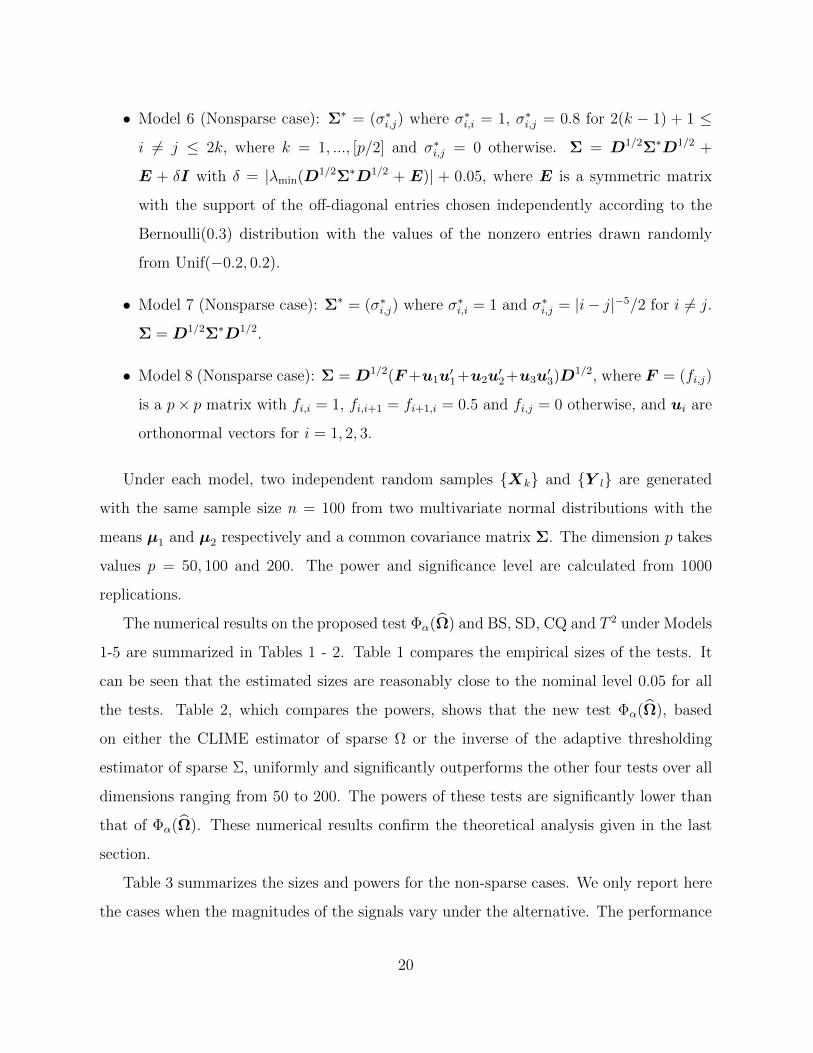
• Model 6 (Nonsparse case): Σ∗ = (σ∗

i,j) where σ∗

i,i= 1, σ∗

i,j= 0.8 for 2(k − 1) + 1 ≤

i = j ≤ 2k, where k = 1, ..., [p/2] and σ∗i,j

= 0 otherwise. Σ = D1/2Σ

∗D1/2 +

E + δI with δ = |λmin(D1/2

Σ∗D1/2 + E)| + 0.05, where E is a symmetric matrix

with the support of the off-diagonal entries chosen independently according to the

Bernoulli(0.3) distribution with the values of the nonzero entries drawn randomly

from Unif(−0.2, 0.2).

• Model 7 (Nonsparse case): Σ∗ = (σ∗i,j) where σ∗

i,i= 1 and σ∗

i,j= |i− j|−5/2 for i = j.

Σ = D1/2Σ

∗D1/2.

• Model 8 (Nonsparse case): Σ = D1/2(F +u1u1+u2u

2+u3u3)D

1/2, where F = (fi,j)

is a p× p matrix with fi,i = 1, fi,i+1 = fi+1,i = 0.5 and fi,j = 0 otherwise, and ui are

orthonormal vectors for i = 1, 2, 3.

Under each model, two independent random samples Xk and Y l are generated

with the same sample size n = 100 from two multivariate normal distributions with the

means µ1 and µ2 respectively and a common covariance matrix Σ. The dimension p takes

values p = 50, 100 and 200. The power and significance level are calculated from 1000

replications.

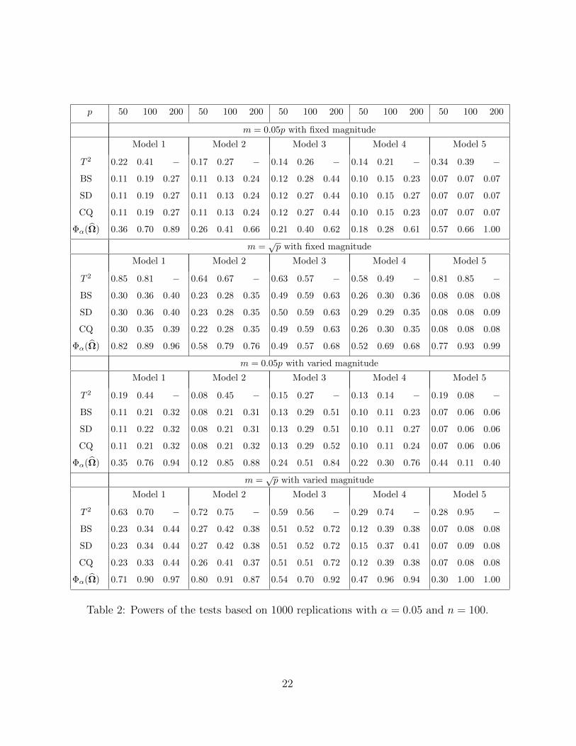
The numerical results on the proposed test Φα(Ω) and BS, SD, CQ and T 2 under Models

1-5 are summarized in Tables 1 - 2. Table 1 compares the empirical sizes of the tests. It

can be seen that the estimated sizes are reasonably close to the nominal level 0.05 for all

the tests. Table 2, which compares the powers, shows that the new test Φα(Ω), based

on either the CLIME estimator of sparse Ω or the inverse of the adaptive thresholding

estimator of sparse Σ, uniformly and significantly outperforms the other four tests over all

dimensions ranging from 50 to 200. The powers of these tests are significantly lower than

that of Φα(Ω). These numerical results confirm the theoretical analysis given in the last

section.

Table 3 summarizes the sizes and powers for the non-sparse cases. We only report here

the cases when the magnitudes of the signals vary under the alternative. The performance

20

p 50 100 200 50 100 200 50 100 200 50 100 200 50 100 200

Model 1 Model 2 Model 3 Model 4 Model 5

T 2 0.04 0.06 − 0.04 0.04 − 0.04 0.05 − 0.05 0.06 − 0.05 0.05 −

BS 0.06 0.07 0.06 0.07 0.06 0.06 0.06 0.05 0.04 0.07 0.07 0.06 0.06 0.06 0.05

SD 0.06 0.07 0.06 0.07 0.06 0.06 0.06 0.05 0.02 0.07 0.07 0.06 0.06 0.06 0.05

CQ 0.06 0.07 0.06 0.06 0.06 0.07 0.06 0.05 0.02 0.07 0.07 0.06 0.06 0.06 0.05

Φα(Ω) 0.05 0.05 0.06 0.04 0.05 0.06 0.05 0.06 0.06 0.04 0.05 0.06 0.03 0.04 0.03

Table 1: Empirical sizes based on 1000 replications with α = 0.05 and n = 100.

of the tests is similar to that in the case of fixed magnitude. It can be seen from Table 3

that the sizes of the sum of square type tests tend to be larger than the nominal level 0.05

while the sizes of the new test Φα(Ω) is smaller than the nominal level. Thus, the new test

has smaller type I error probability than those of the sum of square type tests. For the

models where both Σ and Ω are non-sparse, the power of the proposed test Φα(Ω) is not

as high as in the sparse cases. However, similar phenomena are observed in Table 3 when

comparing the powers with the other tests. The tests based on the sum of squares test

statistics are not powerful against the sparse alternatives, and they are still significantly

outperformed by the new test Φα(Ω).

More extensive simulations were carried out in the non-sparse settings as well as for non-

Gaussian distributions. We also compare the proposed test with the tests based on some

other estimators of the precision matrices. In particular, we consider non-sparse covariance

structures by adding to the covariance/precision matrices in Models 1-5 a perturbation

of a non-sparse matrix E, where E is a symmetric matrix with 30% random nonzero

entries drawn from Unif(−0.2, 0.2). Furthermore, simulations for five additional non-sparse

covariance models are carried out. The comparisons are consistent with the cases reported

here. For reasons of space, these simulation results are given in the supplementary material

Cai, Liu and Xia (2013b).

In summary, the numerical results show that the proposed test Φα(Ω) is significantly

21

p 50 100 200 50 100 200 50 100 200 50 100 200 50 100 200

m = 0.05p with fixed magnitude

Model 1 Model 2 Model 3 Model 4 Model 5

T 2 0.22 0.41 − 0.17 0.27 − 0.14 0.26 − 0.14 0.21 − 0.34 0.39 −

BS 0.11 0.19 0.27 0.11 0.13 0.24 0.12 0.28 0.44 0.10 0.15 0.23 0.07 0.07 0.07

SD 0.11 0.19 0.27 0.11 0.13 0.24 0.12 0.27 0.44 0.10 0.15 0.27 0.07 0.07 0.07

CQ 0.11 0.19 0.27 0.11 0.13 0.24 0.12 0.27 0.44 0.10 0.15 0.23 0.07 0.07 0.07

Φα(Ω) 0.36 0.70 0.89 0.26 0.41 0.66 0.21 0.40 0.62 0.18 0.28 0.61 0.57 0.66 1.00

m =√p with fixed magnitude

Model 1 Model 2 Model 3 Model 4 Model 5

T 2 0.85 0.81 − 0.64 0.67 − 0.63 0.57 − 0.58 0.49 − 0.81 0.85 −

BS 0.30 0.36 0.40 0.23 0.28 0.35 0.49 0.59 0.63 0.26 0.30 0.36 0.08 0.08 0.08

SD 0.30 0.36 0.40 0.23 0.28 0.35 0.50 0.59 0.63 0.29 0.29 0.35 0.08 0.08 0.09

CQ 0.30 0.35 0.39 0.22 0.28 0.35 0.49 0.59 0.63 0.26 0.30 0.35 0.08 0.08 0.08

Φα(Ω) 0.82 0.89 0.96 0.58 0.79 0.76 0.49 0.57 0.68 0.52 0.69 0.68 0.77 0.93 0.99

m = 0.05p with varied magnitude

Model 1 Model 2 Model 3 Model 4 Model 5

T 2 0.19 0.44 − 0.08 0.45 − 0.15 0.27 − 0.13 0.14 − 0.19 0.08 −

BS 0.11 0.21 0.32 0.08 0.21 0.31 0.13 0.29 0.51 0.10 0.11 0.23 0.07 0.06 0.06

SD 0.11 0.22 0.32 0.08 0.21 0.31 0.13 0.29 0.51 0.10 0.11 0.27 0.07 0.06 0.06

CQ 0.11 0.21 0.32 0.08 0.21 0.32 0.13 0.29 0.52 0.10 0.11 0.24 0.07 0.06 0.06

Φα(Ω) 0.35 0.76 0.94 0.12 0.85 0.88 0.24 0.51 0.84 0.22 0.30 0.76 0.44 0.11 0.40

m =√p with varied magnitude

Model 1 Model 2 Model 3 Model 4 Model 5

T 2 0.63 0.70 − 0.72 0.75 − 0.59 0.56 − 0.29 0.74 − 0.28 0.95 −

BS 0.23 0.34 0.44 0.27 0.42 0.38 0.51 0.52 0.72 0.12 0.39 0.38 0.07 0.08 0.08

SD 0.23 0.34 0.44 0.27 0.42 0.38 0.51 0.52 0.72 0.15 0.37 0.41 0.07 0.09 0.08

CQ 0.23 0.33 0.44 0.26 0.41 0.37 0.51 0.51 0.72 0.12 0.39 0.38 0.07 0.08 0.08

Φα(Ω) 0.71 0.90 0.97 0.80 0.91 0.87 0.54 0.70 0.92 0.47 0.96 0.94 0.30 1.00 1.00

Table 2: Powers of the tests based on 1000 replications with α = 0.05 and n = 100.

22

and uniformly more powerful than the other four tests in the settings where either Σ or Ω

is sparse. When both Σ and Ω are non-sparse, the test Φα(Ω) still outperforms the sum of

squares type tests. Based on these numerical results, we recommend using the test Φα(Ω)

with the CLIME estimator of Ω when Ω is known to be sparse and using Φα(Ω) with the

inverse of the adaptive thresholding estimator of Σ when such information is not available.

p 50 100 200 50 100 200 50 100 200

Model 6 Model 7 Model 8

Size

T 2 0.05 0.05 − 0.05 0.05 − 0.04 0.04 −

BS 0.07 0.07 0.05 0.07 0.06 0.05 0.06 0.06 0.06

SD 0.08 0.05 0.05 0.08 0.06 0.05 0.05 0.05 0.06

CQ 0.07 0.07 0.05 0.07 0.06 0.06 0.06 0.06 0.06

Φα(Ω) 0.05 0.05 0.05 0.02 0.02 0.03 0.03 0.02 0.03

Power when m = 0.05p

T 2 0.14 0.37 − 0.17 0.43 − 0.31 0.40 −

BS 0.10 0.22 0.24 0.09 0.12 0.20 0.07 0.10 0.16

SD 0.10 0.21 0.26 0.09 0.13 0.20 0.07 0.09 0.16

CQ 0.10 0.22 0.23 0.09 0.12 0.20 0.07 0.11 0.16

Φα(Ω) 0.16 0.40 0.46 0.14 0.41 0.80 0.20 0.50 0.84

Power when m =√p

T 2 0.47 0.23 − 0.49 0.59 − 0.53 1.00 −

BS 0.17 0.13 0.46 0.16 0.18 0.20 0.11 0.15 0.16

SD 0.14 0.14 0.57 0.16 0.17 0.20 0.12 0.14 0.16

CQ 0.16 0.13 0.46 0.15 0.18 0.20 0.11 0.14 0.16

Φα(Ω) 0.24 0.26 0.77 0.37 0.57 0.53 0.38 0.73 0.85

Table 3: Empirical sizes and powers for Model 6-8 with α = 0.05 and n = 100. Based on

1000 replications.

23

6 Discussions

In the present paper it is assumed that the two populations have the same covariance

matrix. More generally, suppose we observe Xk

iid∼ Np(µ1,Σ1), k = 1, ..., n1, and Y k

iid∼

Np(µ2,Σ2), k = 1, ..., n2 and wish to test H0 : µ1 = µ2 versus H1 : µ1 = µ2. In order to

apply the procedure proposed in this paper, one needs to first test H0 : Σ1 = Σ2 versus

H1 : Σ1 = Σ2. For this purpose, for example, the test introduced in Cai, Liu and Xia

(2013a) can be used. If the null hypothesis H0 : Σ1 = Σ2 is rejected, the test proposed

in this paper is not directly applicable. However, a modified version of the procedure can

still be used. Note that the covariance matrix of X − Y is Σ1/n1 +Σ2/n2. To apply the

test procedure in Section 2, one needs to estimate (Σ1 +n1n2Σ2)−1. When both Σ1 and Σ2

are sparse, the inverse can be estimated well by (Σ1,thr +n1n2Σ2,thr)−1 using the adaptive

thresholding estimators Σ1,thr and Σ2,thr introduced in Cai and Liu (2011). Similarly, when

both Σ1 and Σ2 are bandable, (Σ1+n1n2Σ2)−1 can also be estimated well. A more interesting

problem is the estimation of (Σ1 +n1n2Σ2)−1 when the precision matrices Ω1 and Ω2 are

sparse.

Besides testing the means and covariance matrices of two populations, another inter-

esting and related problem is the testing of the equality of two distributions based on the

two samples. That is, we wish to test H0 : P1 = P2 versus H1 : P1 = P2, where Pi is the

distribution of Np(µi,Σi), i = 1, 2. We shall report the details of the results elsewhere in

the future as a significant amount of additional work is still needed.

The asymptotic properties in Section 3.2 rely on the assumption that the locations of

the nonzero entries of µ1 −µ2 are uniformly drawn from 1, ..., p. When this assumption

does not hold, the asymptotic power results may fail. A simple solution is to first apply a

random permutation to the coordinates of µ1−µ2 (and correspondingly the coordinates of

X − Y ) so that the nonzero locations are uniformly drawn from 1, ..., p, and apply the

testing procedures to the permuted data and the results given in Section 3.2 then hold.

It is well known that the convergence rate in distribution of the extreme value type

statistics is slow. There are several possible ways to improve the rate of convergence. See,

24

for example, Hall (1991), Liu, Lin and Shao (2008) and Birnbaum and Nadler (2012). It is

interesting to investigate whether these methods can be applied to improve the convergence

rate of our test statistic. We leave this to future work.

7 Proof of Main Results

We prove the main results in this section. The proofs of some of the main theorems rely

on a few additional technical lemmas. These technical results are collected in Section 7.1

and they are proved in the supplementary material, Cai, Liu and Xia (2013b).

7.1 Technical Lemmas

Lemma 1 (Bonferroni Inequality). Let A = ∪p

t=1At. For any k < [p/2], we have

2k

t=1

(−1)t−1Et ≤ P(A) ≤2k−1

t=1

(−1)t−1Et,

where Et =

1≤i1<···<it≤pP(Ai1 ∩ · · · ∩ Ait).

Lemma 2 (Berman, 1962). If X and Y have a bivariate normal distribution with expecta-

tion zero, unit variance and correlation coefficient ρ, then

limc→∞

PX > c, Y > c

[2π(1− ρ)12 c2]−1 exp

− c2

1+ρ

(1 + ρ)

12

= 1,

uniformly for all ρ such that |ρ| ≤ δ, for any δ, 0 < δ < 1.

Lemma 3. Suppose (C1) holds and Σ has all diagonal elements equal to 1. Then for

pr-sparse δ, with r < 1/4 and nonzero locations l1, ..., lm, m = pr, randomly and uniformly

drawn from 1, ..., p, we have, for any 2r < a < 1− 2r, as p → ∞,

Pmaxi∈H

(Ωδ)i√ωi,i

−√ωi,iδi

= O(pr−a/2)maxi∈H

|δi|→ 1, (14)

and

Pmaxi∈H

(Ω12δ)i − ai,iδi

= O(pr−a/2)maxi∈H

|δi|→ 1, (15)

25

where Ω12 =: (ai,j) and H is the support of δ.

Lemma 4. Let Yi ∼ N(µi, 1) be independent for i = 1, ..., n. Let an = o((log n)−1/2). Then

supx∈R

max1≤k≤n

Pmax1≤i≤k

Yi ≥ x+ an− P

max1≤i≤k

Yi ≥ x = o(1) (16)

uniformly in the means µi, 1 ≤ i ≤ n. If Yi is replaced by |Yi|, then (16) still holds.

Lemma 5 (Baraud, 2002). Let F be some subset of l2(J). Let µρ be some probability

measure on Fρ = θ ∈ F , θ ≥ ρ and let Pµρ =Pθdµρ(θ). Assuming that Pµρ is

absolutely continuous with respect to P0, we define Lµρ(y) =dPµρ

dP0(y). For all α > 0, ν ∈

[0, 1− α], if E0(L2µρ∗

(Y )) ≤ 1 + 4(1− α− ν)2, then

∀ρ ≤ ρ∗, infΦα

supθ∈Fρ

Pθ(Φα = 0) ≥ ν.

7.2 Proof of Theorem 1

Because we standardize the test statistic first, we shall let (Z1, . . . , Zp)be a zero mean mul-

tivariate normal random vector with covariance matrix Ω = (ωi,j)1≤i,j≤p and the diagonal

ωi,i = 1 for 1 ≤ i ≤ p. To prove Theorem 1, it suffices to prove the following lemma.

Lemma 6. Suppose that max1≤i =j≤p |ωi,j| ≤ r < 1 and maxj

p

i=1 ω2i,j

≤ C0. Then for any

x ∈ R as p → ∞

Pmax1≤i≤p

Z2i− 2 log p+ log log p ≤ x

→ exp

− 1√

πexp(−x/2)

, (17)

Pmax1≤i≤p

Zi ≤

2 log p− log log p+ x

→ exp− 1

2√πexp(−x/2)

. (18)

Proof. We only need to prove (17) because the proof of (18) is similar. Set xp = 2 log p−

log log p+ x. By Lemma 1, we have for any fixed k ≤ [p/2],

2k

t=1

(−1)t−1Et ≤ Pmax1≤i≤p

|Zi| ≥√xp

≤

2k−1

t=1

(−1)t−1Et, (19)

where Et =

1≤i1<···<it≤pP|Zi1 | ≥

√xp, · · · , |Zit | ≥

√xp

=:

1≤i1<···<it≤p

Pi1,··· ,it . De-

fine I =1 ≤ i1 < · · · < it ≤ p : max1≤k<l≤t |Cov(Zik

, Zil)| ≥ p−γ

, where γ > 0 is a

26

sufficiently small number to be specified later. For 2 ≤ d ≤ t− 1, define

Id =1 ≤ i1 < · · · < it ≤ p : Card(S) = d, where S is the largest subset of i1, ..., it

such that ∀ik = il ∈ S, |Cov(Zik, Zil

)| < p−γ

.

For d = 1, define I1 =1 ≤ i1 < · · · < it ≤ p : |Cov(Zik

, Zil)| ≥ p−γ for every 1 ≤ k < l ≤ t

.

So we have I = ∪t−1d=1Id. Let Card(Id) denote the total number of the vectors (i1, . . . , it)

in Id. We can show that Card(Id)≤ Cpd+2γt. In fact, the total number of the subsets of

i1, ..., it with cardinality d is Cd

p. For a fixed subset S with cardinality d, the number of

i such that |Cov(Zi, Zj)| ≥ p−γ for some j ∈ S is no more than Cdp2γ. This implies that

Card(Id)≤ Cpd+2γt. Define Ic = 1 ≤ i1 < · · · < it ≤ p \ I. Then the number of elements

in the sum

(i1,··· ,it)∈Ic Pi1,··· ,it is Ct

p−O(

t−1d=1 p

d+2γt) = Ct

p−O(pt−1+2γt) = (1 + o(1))Ct

p.

To prove Lemma 6, it suffices to show that

Pi1,··· ,it = (1 + o(1))π− t2p−t exp(−tx

2) (20)

uniformly in (i1, . . . , it) ∈ Ic, and for 1 ≤ d ≤ t− 1,

(i1,··· ,it)∈Id

Pi1,··· ,it → 0. (21)

Putting (19) - (21) together, we obtain that

(1 + o(1))S2k ≤ Pmax1≤i≤p

|Zi| ≥√xp

≤ (1 + o(1))S2k−1, (22)

where Sk =

k

t=1(−1)t−1 1t!π

− t2 exp(− tx

2 ). Note that limk→∞ Sk = 1 − exp(− 1√πe−x/2). By

letting p → ∞ first and then k → ∞ in (22), we prove Lemma 6.

We now prove (20). Let z = (zi1 , ..., zit) and |z|min = min1≤j≤t |zij |. Write

Pi1,··· ,it =1

(2π)t/2det(Ωt)12

|z|min≥√xp

exp(−1

2zΩ

−1tz)dz,

where Ωt is the covariance matrix of Z = (Zi1 , ..., Zit), and Ωt = (akl)t×t, where akl =

Cov(Zik, Zil

). Since i1, ..., it ∈ Ic, ak,k = 1 and |akl| < p−γ for k = l. Write

|z|min≥√xp

exp(−1

2zΩ

−1tz)dz =

|z|min≥√xp,z2>(log p)2

exp(−1

2zΩ

−1tz)dz

27

+

|z|min≥√xp,z2≤(log p)2

exp(−1

2zΩ

−1tz)dz. (23)

Then

|z|min≥√xp,z2>(log p)2

exp(−1

2zΩ

−1tz)dz ≤ C exp(−(log p)2/2t) ≤ Cp−2t, (24)

uniformly in (i1, . . . , it) ∈ Ic. For the second part of the sum in (23), note that

Ω−1t

− I2 ≤ Ω−1t2Ωt − I2 ≤ Cp−γ. (25)

Let A = |z|min ≥ √xp, z2 ≤ (log p)2. It follows that

A

e−12z

Ω−1t zdz =

A

e−12z

(Ω−1t −I)z− 1

2z2dz

= (1 +O(p−γ(log p)2))

A

e−12z

2dz

= (1 +O(p−γ(log p)2))

|z|min≥√xp

e−12z

2dz + Cp−2t, (26)

uniformly in (i1, . . . , it) ∈ Ic. This, together with (23) and (24), implies (20).

It remains to prove (21). For S ⊂ Id with d ≥ 1, without loss of generality, we can

assume S = it−d+1, ..., it. By the definition of S and Id, for any k ∈ i1, . . . , it−d, there

exists at least one l ∈ S such that |Cov(Zk, Zl)| ≥ p−γ. We divide Id into two parts:

Id,1 =1 ≤ i1 < · · · < it ≤ p : there exists an k ∈ i1, . . . , it−d such that

for some l1, l2 ∈ S with l1 = l2, |Cov(Zk, Zl1)| ≥ p−γ and |Cov(Zk, Zl2)| ≥ p−γ

and Id,2 = Id \ Id,1. Clearly, I1,1 = ∅ and I1,2 = I1. Moreover, we can show that

Card(Id,1)≤ Cpd−1+2γt. For any (i1, . . . , it) ∈ Id,1,

P|Zi1 | ≥

√xp, . . . , |Zit | ≥

√xp

≤ P

|Zit−d+1

| ≥ √xp, . . . , |Zit | ≥

√xp

= O(p−d).

Hence by letting γ be sufficiently small,

Id,1

Pi1,··· ,it ≤ Cp−1+2γt = o(1). (27)

28

For any (i1, . . . , it) ∈ Id,2, without loss of generality, we assume that |Cov(Zi1 , Zit−d+1)| ≥

p−γ. Note that

P|Zi1 | ≥

√xp, . . . , |Zit | ≥

√xp

≤ P

|Zi1 | ≥

√xp, |Zit−d+1

| ≥ √xp, . . . , |Zit | ≥

√xp

.

Let U l be the covariance matrix of (Zi1 , Zit−d+1, . . . , Zit). We can show that U l − U l2 =

O(p−γ), where U l = diag(D, Id−1) and D is the covariance matrix of Zi1 and Zit−d+1. Using

the similar arguments as in (23)-(26), we can get

P|Zi1 | ≥

√xp, |Zit−d+1

| ≥ √xp, . . . , |Zit | ≥

√xp

≤ (1 + o(1))P(|Zi1 | ≥√xp, |Zit−d+1

| ≥ √xp)×O(p−d+1) ≤ Cp−

21+r ×O(p−d+1),

where the last inequality follows from Lemma 2 and the assumption max1≤i =j≤p |ωi,j| ≤

r < 1. Thus by letting γ be sufficiently small,

Id,2

Pi1,··· ,it ≤ Cpd+2γt−d+1− 21+r = o(1). (28)

Combining (27) and (28), we prove (21). The proof of Lemma 6 is then complete.

7.3 Proof of Theorem 2

It suffices to prove Pmax1≤i≤p

(Ωδ)i/√ωi,i

≥(2 + ε/2) log p/n

→ 1. By Lemma

3 and the condition maxi |δi/σ12i,i| ≥

2β log p/n with β ≥ 1/(mini σi,iωi,i) + ε for some

constant ε > 0, we can get max1≤i≤p |(Ωδ)i/√ωi,i| ≥

(2 + ε/2) log p/n with probability

tending to one. So Theorem 2 follows.

7.4 Proof of Theorem 3

First we assume kp = o(pr) for some r < 1/4, and we can get similar argument if kp = O(pr)

for some r < 1/2 and Ω = Σ−1 is sp sparse with sp = O((p/k2

p)γ) for some 0 < γ < 1. Let

Ms,p denote the set of all subsets of 1, ..., p with cardinality kp. Let m be a random set

of 1, ..., p, which is uniformly distributed on M. Let ωj, 1 ≤ j ≤ p be i.i.d. variables

with P(ωj = 1) = P(ωj = −1) = 1/2. We construct a class of δ = µ1 − µ2 by letting

29

µ1 = 0 and δ = −µ2 satisfy δ = (δ1, . . . , δp)with δj =

ρ√kpωj1j∈m, where ρ = c

kp log p

n

and c > 0 is sufficiently small that will be specified later. Clearly, |δ|2 = ρ. Let µρ be

the distribution of δ. Note that µρ is a probability measure on δ ∈ Skp : |δ| = ρ. We

now calculate the likelihood ratio Lµρ =dPµρ

dP0(Xn,Y n). It is easy to see that Lµρ =

Em,ω

exp(−

√nZ

δ− n

2δΩδ)

, where Z is a multivariate normal vector with mean 0 and

Cov(Z) = Ω, and is independent with m and Ω. For any fixed m = m, let δi

m, 1 ≤ i ≤ 2kp

be all the possible values of δ. That is, Pδ = δi

m|m = m

= 2−kp . Thus

Em,ω

exp(−

√nZ

δ − n

2δΩδ)

=

1p

kp

1

2kp

m∈M

2kp

i=1

exp−

√nZ δ(i)

(m) −n

2δ(i)

(m)Ωδ(i)(m)

.

It follows that

EL2µρ

= E 1

p

kp

1

2kp

m∈M

2kp

i=1

exp−

√nZ δ(i)

(m) −n

2δ(i)

(m)Ωδ(i)(m)

2

=1

p

kp

21

22kpE

m,m∈M

2kp

i,j=1

exp−√nZ (δ(i)

(m) + δ(j)(m))−

n

2(δ(i)

(m)Ωδ(i)(m) + δ(j)

(m)Ωδ(j)(m))

=1

p

kp

21

22kp

m,m∈M

2kp

i,j=1

exp

− n

2(δ(i)

(m)Ωδ(i)(m) + δ(j)

(m)Ωδ(j)(m))

× expn2(δ(i)

(m) + δ(j)

(m))Ω(δ(i)(m) + δ(j)

(m))

=1

p

kp

21

22kp

m,m∈M

2kp

i,j=1

expnδ(i)

(m)Ωδ(j)(m)

=

1p

kp

21

22kp

m,m∈M

2kp

i,j=1

expnρ2

kp

k∈m,l∈m

ak,lω(i)kω(j)l

,

where ρ√kp(ω(i)

kIk∈m) := δ(i)

(m) and Ω = (akl)p×p. Thus

EL2µρ

=1

p

kp

21

22kp

m,m∈M

2kpkp

k,l=1

exp(

nρ2

kpakl) + exp(−nρ2

kpakl)

=1

p

kp

2

m,m∈M

k∈m,l∈m

cosh(nρ2

kpakl) ≤

1p

kp

2

m,m∈M

k∈m,l∈m

expnρ2

kp|akl|

.

For every m, let B := Bm = l : |ak,l| ≥ M

d, k ∈ m, where d =

p

k2p

1−γ

and γ is

sufficiently small. For every k, the number of l such that |akl| ≥ M

dis at most d. Hence

EL2µρ

≤ 1p

kp

2

m∈M

kp

j=0

I|m ∩ B| = j exp

k∈m,l∈m

nρ2

kp|akl|

30

=1

p

kp

2

m∈M

kp

j=0

I|m ∩ B| = j exp

k∈m,l∈m∩B

nρ2

kp|akl|+

k∈m,l∈m∩Bc

nρ2

kp|akl|

≤ 1p

kp

2

m∈M

kp

j=0

kpd

j

p− kpkp − j

exp

Mnρ2

kpj +

Mk2plog p

d

≤ 1p

kp

kp

j=0

kpd

j

p− kpkp − j

exp

Mnρ2

kpj +

Mk2plog p

d

≤ (1 + o(1))

kp

j=0

kpj

(dkp)j

pjexp

Mnρ2

kpj +

Mk2plog p

d

= (1 + o(1))1 +

dkpt

p

kp

expMk2

plog p

d

,

where t = exp

Mnρ2

kp

= pMc

2. It follows that

EL2µρ

≤ (1 + o(1)) expkp log

1 +

dkpt

p

+

Mk2plog p

d

≤ (1 + o(1)) expkp

dkpt

p+

Mk2plog p

d

≤ 1 + 4(1− α− ν)2

by letting c be sufficiently small. If kp = O(pr) for some r < 1/2 and Ω = Σ−1 is sp sparse

with sp = O((p/k2p)γ) for some 0 < γ < 1, we let B := Bm = l : ak,l = 0, k ∈ m. Then

we can similarly get

EL2µρ

≤ 1p

kp

2

m∈M

kp

j=0

I|m ∩B| = j exp

k∈m,l∈m

nρ2

kp|akl|

≤ 1p

kp

2

m∈M

kp

j=0

I|m ∩B| = j expMnρ2

kpj≤ (1 + o(1))

1 +

spkpt

p

kp

,

So we can still get EL2µρ

≤ 1 + 4(1− α − ν)2 by letting c be sufficiently small. Theorem 3

now follows from Lemma 5.

7.5 Proof of Theorem 4

We only prove part (ii) of Theorem 4 in this section, part (i) follows from the proof of part

(ii) directly. Without loss of generality, we assume that σi,i = 1 for 1 ≤ i ≤ p. Define the

31

event A = max1≤i≤p |δi| ≤ 8

log p/n. By conditions in Theorem 4, we have

max1≤i≤p

|ω(0)i,i

− ωi,i| = oP(1/ log p).

Hence, as in the proof of Proposition 1 (i) in the supplement material, it is easy to show

that PMΩ ∈ Rα,A

c

= P(Ac) + o(1) and P

MΩ ∈ Rα,A

c

= P(Ac) + o(1). Note that

Ω(X − Y ) = (Ω−Ω)(X − Y − δ) + (Ω−Ω)δ +Ω(X − Y ). On A, we have

(Ω−Ω)(X − Y − δ) + (Ω−Ω)δ∞

= oP 1√

n log p

.

To prove Theorem 4, it suffices to show that

Pmax1≤i≤p

|Zo

i| ≥ √

xp + an,A= P

max1≤i≤p

|Zo

i| ≥ √

xp,A+ o(1), (29)

for any an = o((log p)−1/2), where Zo

i= (ΩZ)i/

√ωi,i defined in the proof of Proposition

1 (i) in the supplement material. From the proof of Proposition 1 (i), let H = supp(δ) =

l1, ..., lpr, then we can get

Pmax1≤i≤p

|Zo

i| ≥ √

xp + an,A= αP(A) + (1− α)P(max

i∈H|Yi| ≥

√xp + an,A) + o(1),

Pmax1≤i≤p

|Zo

i| ≥ √

xp,A= αP(A) + (1− α)P(max

i∈H|Yi| ≥

√xp,A) + o(1),

where given δ, Yi, i ∈ H are independent normal random variables with unit variance.

This, together with Lemma 4, implies (29).

7.6 Proof of Theorem 6

Let (V1, ..., Vp) be a zero mean random vector with covariance matrix Ω = (ωi,j) and

the diagonal ωi,i = 1 for 1 ≤ i ≤ p satisfying moment conditions (C6) or (C7). Let

Vli = VliI|Vli| ≤ τn for l = 1, ..., n, where τn = η−1/22

log(p+ n) if (C6) holds and

τn =√n/(log p)8 if (C7) holds. Let Wi =

n

l=1 Vli/√n and Wi =

n

l=1 Vli/√n. Then

P(max1≤i≤p

|Wi − Wi| ≥1

log p) ≤ P(max

1≤i≤p

max1≤l≤n

|Vli| ≥ τn) ≤ np max1≤i≤p

P(|V1i| ≥ τn) = O(p−1 + n−/8).(30)

Note that

max1≤i≤p

W 2i− max

1≤i≤p

W 2i

≤ 2 max1≤i≤p

|Wi| max1≤i≤p

|Wi − Wi|+ max1≤i≤p

|Wi − Wi|2. (31)

32

By (30) and (31), it is enough to prove that for any x ∈ R, as p → ∞

P(max1≤i≤p

W 2i− 2 log p+ log log p ≤ x) → exp(− 1√

πexp(−x

2)).

It follows from Lemma 1 that for any fixed k ≤ [p/2],

2k

t=1

(−1)t−1

1≤i1<...<it≤p

P(|Wi1 | ≥ xp, ..., |Wit | ≥ xp) ≤ P(max1≤i≤p

|Wi| ≥ xp)

≤2k−1

t=1

(−1)t−1

1≤i1<...<it≤p

P(|Wi1 | ≥ xp, ..., |Wit | ≥ xp). (32)

Define |W |min = min1≤l≤t |Wil|. Then by Theorem 1 in Zaitsev (1987), we have

P(|W |min ≥ xp) ≤ P(|Z|min ≥ xp − n(log p)−1/2) + c1d

5/2 exp(− n12 n

c2d3τn(log p)12

), (33)

where c1 > 0 and c2 > 0 are absolute constants, n → 0 which will be specified later

and Z = (Zi1 , ..., Zit) is a t dimensional normal vector as defined in Theorem 1. Because

log p = o(n1/4), we can let → 0 sufficiently slow such that

c1d5/2 exp(− n

12 n

c2d3τn(log p)12

) = O(p−M) (34)

for any large M > 0. It follows from (32), (33) and (34) that

P(max1≤i≤p

|Wi| ≥ xp) ≤2k−1

t=1

(−1)t−1

1≤i1<...<it≤p

P(|Z|min ≥ xp − n(log p)−1/2) + o(1). (35)

Similarly, using Theorem 1 in Zaıtsev (1987) again, we can get

P(max1≤i≤p

|Wi| ≥ xp) ≥2k

t=1

(−1)t−1

1≤i1<...<it≤p

P(|Z|min ≥ xp − n(log p)−1/2)− o(1). (36)

So by (35), (36) and the proof of Theorem 1, the theorem is proved.

7.7 Proof of Theorem 7

(i). (i) follows from the proof of Theorem 4.

33

(ii). Note that Ω(X−Y ) = (Ω−Ω)(X−Y −δ)+(Ω−Ω)δ+Ω(X−Y ). It suffices to prove

Pmax1≤i≤p

√n(Ωδ)i/

√ωi,i+

√nΩ(X − Y − δ)i/

√ωi,i

≥√ρ log p

→ 1 for some ρ > 2.

To this end, we only need to show Pmax1≤i≤p

(Ωδ)i/√ωi,i

≥(2 + ε/4) log p/n

→ 1.

Note that

max1≤i≤p

|(Ωδ)i/√ωi,i| ≥ max

1≤i≤p

|(Ωδ)i/√ωi,i|+ oP(1) max

1≤i≤p

|δi| ≥ (1 + oP(1)) max1≤i≤p

|(Ωδ)i/√ωi,i|.

By the condition maxi |δi/σ12i,i| ≥

2β log p/n with β ≥ 1/(mini σi,iωi,i) + ε for some con-

stant ε > 0, we can get max1≤i≤p |(Ωδ)i/√ωi,i| ≥

(2 + ε/2) log p/n with probability

tending to one. This proves (ii).

Acknowledgements

The authors would like to thank the Associate Editor and three referees for their helpful

constructive comments which have helped to improve quality and presentation of the paper.

This research was supported in part by NSF FRG Grant DMS-0854973. Weidong Liu’s

research was also supported by NSFC, Grant No.11201298, the Program for Professor

of Special Appointment (Eastern Scholar) at Shanghai Institutions of Higher Learning,

Foundation for the Author of National Excellent Doctoral Dissertation of PR China and

the startup fund from SJTU.

References

[1] Anderson, T.W. (2003). An introduction to multivariate statistical analysis. Third

edition. Wiley-Interscience.

[2] Arias-Castro, E., Candes, E. and Plan, Y. (2011). Global Testing under Sparse Al-

ternatives: ANOVA, Multiple Comparisons and the Higher Criticism. Ann. Statist.

39:2533-2556.

34

[3] Bai, Z. and Saranadasa, H. (1996). Effect of high dimension: by an example of a two

sample problem. Statist. Sinica 6:311-329.

[4] Baraud, Y. (2002). Non-asymptotic minimax rates of testing in signal detection.

Bernoulli 8:577-606.

[5] Berman, S.M. (1962). A law of large numbers for the maximum of a stationary Gaus-

sian sequence. Ann. Math. Statist. 33:93-97.

[6] Berman, S.M. (1964). Limit theorems for the maximum term in stationary sequences.

Ann. Math. Statist. 35:502-516.

[7] Bickel, P. and Levina, E. (2008). Covariance regularization by thresholding. Ann.

Statist. 36:2577-2604.

[8] Birnbaum, A. and Nadler, B. (2012). High dimensional sparse covariance estimation:

accurate thresholds for the maximal diagonal entry and for the largest correlation

coefficient. Technical Report.

[9] Cai, T. and Liu, W.D. (2011). Adaptive thresholding for sparse covariance matrix

estimation. J. Amer. Statist. Assoc. 106:672-684.

[10] Cai, T., Liu, W.D. and Luo, X. (2011). A constrained l1 minimization approach to

sparse precision matrix estimation. J. Amer. Statist. Assoc. 106:594-607.

[11] Cai, T., Liu, W.D. and Xia, Y. (2013a). Two-Sample covariance matrix testing and

support recovery in high-dimensional and sparse settings. J. Amer. Statist. Assoc.,

108: 265-277.

[12] Cai, T., Liu, W.D. and Xia, Y. (2013b). Supplement to “Two-Sample test of high

dimensional means under dependency”. Technical report.

[13] Cai, T. and Yuan, M. (2012). Adaptive covariance matrix estimation through block

thresholding. Ann. Statist. 40: 2014-2042.

35

[14] Cai, T. and Zhou, H. (2012). Minimax estimation of large covariance matrices under

1 norm (with discussion). Statist. Sinica 22:1319-1378.

[15] Cai, T., Zhang, C.-H. and Zhou, H. (2010). Optimal rates of convergence for covariance

matrix estimation. Ann. Statist. 38: 2118-2144.

[16] Cao, J. andWorsley, K.J. (1999). The detection of local shape changes via the geometry

of Hotelling’s T 2 fields. Ann. Statist. 27:925-942.

[17] Castagna J. P., Sun S., and Siegfried R. W. (2003). Instantaneous spectral analysis:

Detection of low-frequency shadows associated with hydrocarbons. The Leading Edge

22:120-127.

[18] Chen, S. and Qin, Y. (2010). A two-sample test for high-dimensional data with appli-

cations to gene-set testing. Ann. Statist. 38:808-835.

[19] Hall, P. (1991). On convergence rates of suprema. Probab. Theory Related Fields

89:447-455.

[20] Hall, P. and Jin, J. (2008). Properties of higher criticism under strong dependence.

Ann. Statist. 36:381-402.

[21] Hall, P. and Jin, J. (2010). Innovated higher criticism for detecting sparse signals in

correlated noise. Ann. Statist. 38:1686-1732.

[22] James D., Clymer B. D., and Schmalbrock P. (2001). Texture detection of simulated

microcalcification susceptibility effects in magnetic resonance imaging of breasts. J.

Magn. Reson. Imaging 13:876-881.

[23] Liu, W., Lin, Z.Y. and Shao, Q.M. (2008), The asymptotic distribution and Berry-

Esseen bound of a new test for independence in high dimension with an application

to stochastic optimization. Ann. Appl. Probab. 18:2337-2366.

36

[24] Ravikumar, P., Raskutti, G., Wainwright, M.J. and Yu, B. (2008). Model selection in

Gaussian Graphical Models: high-dimensional consistency of l1-regularized MLE. In

Advances in Neural Information Processing Systems (NIPS) 21.

[25] Rothman, A., Bickel, P., Levina, E. and Zhu, J. (2008). Sparse permutation invariant

covariance estimation. Electron. J. Statist. 2:494-515.

[26] Srivastava, M. and Du, M. (2008). A test for the mean vector with fewer observations

than the dimension. J. Multivariate Anal. 99:386-402.

[27] Srivastava, M. (2009). A test for the mean vector with fewer observations than the

dimension under non-normality. J. Multivariate Anal. 100:518-532.

[28] Taylor, J.E. and Worsley, K.J. (2008). Random fields of multivariate test statistics,

with applications to shape analysis. Ann. Statist. 36:1-27.

[29] Yuan, M. (2010). High dimensional inverse covariance matrix estimation via linear

programming. J. Mach. Learn. Res. 11:2261-2286.

[30] Yuan, M. and Lin, Y. (2007). Model selection and estimation in the gaussian graphical

model. Biometrika 94:19-35.

[31] Zaıtsev, A. Yu. (1987), On the Gaussian approximation of convolutions under multidi-

mensional analogues of S.N. Bernstein’s inequality conditions. Probab. Theory Related

Fields 74:535-566.

[32] Zhang G., Zhang S., and Wang Y. (2000). Application of adaptive time-frequency

decomposition in ultrasonic NDE of highly-scattering materials. Ultrasonics 38:961-

964.

37