European Riches Select and European Riches November 21, 2019

Two Roads to Riches? The (In)Frequency of Strongly Disruptive
Technological Change
Kenneth L. Simons
Department of Economics Rensselaer Polytechnic Institute
110 8th Street Troy, NY 12180-3590
United States Tel.: 1 518 276 3296
Email: [email protected] Web: www.rpi.edu/~simonk
version 10 November 2009 The author thanks the Ewing Marion Kauffman Foundation for financial support. Research assistance was provided by Chris Mega, Chunbo Ma, Emily Gatt, Bharath Krishnamurthy, Rob Walker, Angela Tan, Vanessa Wong, Kara Chesal, Chris Livingston, Sanzhar Kenzhekhanuly, Karl Rogler, Jenny Martos, Derek Cutler, Paul Gale, Jaime Potter, Jose Pallares, Ashwin Krishna, Hareesh Bajaj, Katherine Lawler, Kenneth Galarneau, Diego Regules, Jeremy Walker, Phillip Harris, Robert DeVida, plus about twenty Carnegie Mellon undergraduates in 1991-1994. The Carnegie Mellon and RPI interlibrary loan offices, Carol Rizzo and Pamela Murarka, Steven Klepper, and Dongling Huang all provided invaluable assistance. Participants at conferences and seminars of the Academy of Management, the Atlanta Competitive Advantage Conference, the Industry Studies Association, the International Industrial Organization Society, the WUN Global Entrepreneurship Initiative, and Purdue University provided helpful comments.

1
Two Roads to Riches? The (In)Frequency of Strongly Disruptive Technological Change
Abstract: The frequency with which radical technological changes disrupt industry competition is an open question. The present paper develops an upper-bound estimate of the frequency of “strong” disruptive technological changes within defined product industries. This estimate is obtained by searching not for subjectively-defined radical technological changes, as past studies have done for particular industries, but for objectively-defined effects of radical technological changes on firm entry and survival patterns. Strong disruptive technological changes are defined as those that lead to replacement of (at least some) incumbent firms by new entrants, and hence imply detectable patterns in firm entry and exit. Data spanning many decades and 47 product-level industries, detailing firm entry and exit in each industry, are used to assess the frequency of disruptive entry and exit patterns and hence to bound the frequency of strong disruptive technological change within industries. Periods of strong disruption turn out to occur in the data approximately as often as would be expected given random fluctuations of entry and exit. Hence strong disruptive technological change within industries appears to be a rare phenomenon. Assuming that disruptive technological changes are in fact frequent, this suggests that disruptive technological changes typically are not associated with Schumpeterian surges in entry and exit. Keywords: industry dynamics, technology, disruptive technology, radical technological change
“[T]ransformational technologies are very rare – on the order of every three or four decades….
There has been a tendency to dramatically overstate the disruptive impact of technologies.”
Michael Porter (Argyres and McGahan, 2002, p. 48)
I. Introduction
Research on technology and industries has identified two roads to riches. Firms can earn
profits by creating or imitating a new product technology, which fills a need as yet unfulfilled.
Alternatively, firms can earn profits by developing or imitating a replacement technology, which
improves on and replaces technology already commercialized by established firms. How often
these two roads to riches are successfully employed depends on relative abilities of entrant and
incumbent firms.

2
The balance of power between established firms and entrepreneurial entrants depends on
evolving technology. Competence-enhancing versus competence-destroying technological
changes, as Tushman and Anderson (1986) put it, respectively help or harm established firms.
Times with competence-enhancing technological change correspond to early-mover advantage,
and times of competence-destroying technological change correspond to late-mover advantage,
explaining some of the varied findings in the literature on early- and late-mover advantage (cf.,
Lieberman and Montgomery, 1998; Schnaars, 1994). That technological change and innovation
can provide entrant firm advantage has long been recognized, in economics (cf., Reinganum,
1983) and in managerial strategy (cf., Cooper and Schendel, 1976; Foster, 1986). Disruptive
technological change, popularized in the business press by Christensen (1997), is often defined
as competence-destroying technological change for which entrants succeed at displacing
established firms. For example, Kasper Instruments, the 1973 market leader in photolithographic
alignment equipment, lost its market share to Perkin-Elmer in the mid-1970s transition to
proximity aligners and exited in 1981 (Henderson and Clark 1990; Henderson 1993).
This paper analyzes how business ventures fare in a wide range of product markets, and
asks how often ventures are attracted by radical new technologies that strongly disrupt industry
competition by allowing the entrants to take over existing markets. To answer this question, this
paper takes a deliberately indirect approach. Detailed information about relevant technologies is
difficult to obtain and often involves subjective interpretation. In contrast, detectable
implications of strong disruptive technological change on competition are unambiguous: firms
should enter a market and outcompete its incumbent firms.
The present paper checks how often any unusual amount of entry occurs, and in the
aftermath of that entry, whether the new entrants disproportionately choose to remain in the

3
industry while incumbents tend to exit. Thus it checks for strong disruption. Weak disruption,
not detected here, might involve market share change without market exit, successful innovation
by small incumbents instead of by market entrants, or successful innovation by new divisions of
incumbents. If the patterns of strong disruption are the norm, then ventures into a new area of
business might frequently use new technologies as the means to coups in which they take away
market profitability from incumbent firms.
Hence, this paper estimates an upper bound to the frequency of strong disruptive
technological change in specific industries, by searching not subjectively for the responsible
technologies, but objectively for the patterns of disruption. The thumbprint of a strong disruptive
technological change is an abrupt wave of entry followed by a wave of exit of incumbent firms,
relative to normal rates of entry and exit. If this thumbprint of strong disruption occurs, it says
nothing about whether technology versus some other factor caused the disruption. Hence the
frequency estimated can be taken only as an upper bound. If the estimated upper bound is low,
that would suggest that strongly disruptive technological change is rare in specific industries, and
one could go further to investigate any specific instances of strong disruption found to see
whether they seem to involve important new technologies used by entering firms.
The sample of firms studied here consists of U.S. manufacturers of 47 products over the
1900s. The data define industries narrowly enough that firms generally are in direct competition
with each other; that is, their products are largely substitutable from the viewpoint of the
consumer, ensuring that they actually compete with each other. The data provide good evidence
about new ventures, including small firms, and how they fared in their new competitive
environments. The competitive environments considered span a wide range of technology types

4
and historical eras, and thus are likely to be reasonably representative of the cross-section of at
least manufacturing industry competitive dynamics.
This analysis of the frequency of disruptive technological change is limited to a particular
type of disruption: that in which new firms replace old firms. Hence the search is for a strong
rather than weak form of technological disruption, not merely new firms gaining market share
greater than that of old firms. The literature on disruptive technological change suggests that just
this sort of strong replacement of firms, rather than merely relatively weak movements of market
share, occurs in practice. And given the large number of producers in the industries studied here,
it is natural to expect that a substantial advance in market share by an entering firm is likely to
put out of business some of the incumbents.
The analysis is also limited to a particular context: the continuing industry. Industries are
defined by the practical categories used to define products in trade directories, and these
definitions rule out instances in which the very names of products change dramatically, as from
vacuum tubes to transistors. The literature on disruptive technological change suggests ample
examples of disruptive changes that occurred within continuing product-defined industries of this
kind, and argues that firms need to be ready for disruptive technology-driven change even when
there is no technology on the horizon that would create an entirely different product that serves
the same purpose. Hence it is of great interest to investigate the frequency of disruptive
technological change in continuing industries. Of course greater rates of industry disruption
might be observed when replacement technologies arise that are so novel that they in fact replace
the old product with something totally new, and the study of this broader phenomenon must
await even more involved datasets, still retaining narrow product-level definitions of industries,
than the data used here.

5
The analysis further is limited to a particular time span: the 1900s, with relatively little
evidence on the 1980s and 1990s. One might wonder whether the pace of technological
replacement of incumbent firms has increased over time and is now especially important even if
it was not as important in past. A check on this idea is carried out by testing whether there has
been a change in the frequency of disruptive technological change with regard to calendar time
during the period studied.
Albeit the above constraints on the analysis, it is extremely valuable to enhance our
understanding of the nature of technological change – and particularly disruptive technological
change – in industries. Strongly disruptive technological change, judging from the evidence
presented herein, turns out apparently to be very rare. Among the 48 industries studied over
periods of many decades, the number of instances of entry and exit patterns that match disruption
is in fact almost exactly the number that would be expected given random fluctuations of entry
and exit. Technology is exceedingly important to firms’ competitive positions in many of the
industries studied here, but it seems largely to be important in a non-disruptive manner: in many
industries firms must maintain their technological strengths to remain viable given ongoing
competition, and in practice the firms that win this competitive battle are often disproportionately
the incumbents. While technology is often crucial to the competitive process, it seems that
strongly disruptive technological change within industries is an unusual phenomenon. If one
presumes that technological disruptions of some kind are in fact rather frequent, then this
suggests that these disruptions typically are not associated with Schumpeterian waves of entry
and exit in industries.

6
II. Alternative Competitive Patterns
A. Radical Technological Change and Disruption
Radical technological change, a growing literature has shown, has the potential to disrupt
industry structure. New firms taking the right advantage of the right technology can unseat
incumbent producers, driving them out of the business and replacing them as providers of the
customers’ need. In economics, the best-known literature focuses on a monopolist challenged by
an entrant using a new technology. Arrow (1962) pointed out that a monopolist has less
incentive to develop a novel product or process technology than does an entrant which could
gain a monopoly by developing the same technology. In contrast, the theoretical work of Gilbert
and Newberry (1982) showed that monopolists should defend their markets through preemptive
patenting and other defensive behaviors. However, Reinganum (1983) proved that such strong
defensive behavior is not universal. If the time when the new technology emerges is random and
tends to occur sooner when greater R&D investments are made, and if the advantage of the new
technology is drastic relative to the cost (or quality) advantages of the old technology, then new
firms have greater incentive to invest in the new technology than incumbents, and entrants are
likely to replace incumbents.
There are many examples of a replacement technology causing replacement of producers
of a product. The replacement of vacuum tube producers by transistor manufacturers is a classic
example. Similarly, mechanical calculator producers fell to new makers of electronic calculators
(Majumdar, 1982). In management research, the loss of at least market share and usually also
market survival to upstart firms has been blamed on technologies in a range of industries: a
patented cement manufacturing process that burned powdered coal as fuel and the use of
integrated circuits for minicomputers (Tushman and Anderson 1986); several generations of

7
semiconductor lithographic alignment techniques starting from physical contact between mask
and wafer and moving to proximity, scanning optics, and two generations of step-by-step
alignment (Henderson and Clark 1990; Henderson 1993); and successive generations of sizes in
computer hard disks (Christensen and Rosenbloom 1995; Christensen 1997). Schnaars (1994)
catalogs 28 cases in which imitators surpassed early market pioneers, sometimes aided by new
technologies.
Conditions under which technological disruptions are likely to arise, or incumbents are
likely to fail as a result of disruptive technology, have been analyzed in a series of research
works. Adner (2002) and Adner and Zemsky (2005) analyze how demand structure may impact
disruptive change. Schivardi and Schneider (2008) consider the combined effects of uncertainty
in technological potential and of learning curves. Gans, Hsu, and Stern (2002) uncover
conditions under which cooperative development rather than disruptive entry are likely to arise.
Tripsas (1997a) highlights benefits of knowledge absorption capabilities and of dynamic
capabilities created through geographic diversity to help incumbents survive disruptions. Tripsas
(1997b) and Rothaermel and Hill (2005) analyze the importance of complementary assets to
incumbent survival. Tripsas and Gavetti (2000), among others, analyze how managerial
perceptions condition incumbents’ decisions to invest in a disruptive technology.
Christensen (1997) particularly has argued that companies must properly manage new
technologies, to innovate or fail. Surely it is useful for firms to pay attention to potential
technological threats. However, if firms are choosing a level of response to technological
threats, it is possible to choose a level of response that is too high as well as one that is too low.
Given the enormous financial commitments involved in new technology development, and the
ramifications of these commitments for shareholders and for society at large, it is important to

8
understand better the frequency with which new technological threats in fact materialize.
Numerous technologies failed to replace existing products, and many defensive R&D efforts
turned out to be unnecessary. Accordingly the informed decision maker who seeks to maximize
either corporate or societal gains must weigh the costs of inaction against the costs of action.1
This suggests reason for caution when interpreting the extent to which disruptive technological
change should be a preeminent concern.2
B. Continual Technological Change and Concentration
Disruptive technological change is by no means the only sort of technological change, for
continuous technological change, related to pre-existing technologies, has been well-documented
in many more industries. Tushman and Anderson (1986), in a classic article in the management
literature, distinguish competence-destroying versus competence-enhancing technological
change, and argue that the former tends to destroy market leadership of incumbent firms while
the latter enhances market leadership of incumbent firms. Their characterization suggests that
technology enhances competence when it is similar to technology already used by incumbents.
A recent literature in economics documents patterns of increasing concentration in
number of firms and market share. Gort and Klepper (1982) show that most U.S. manufactured
products seem to experience an initial buildup in their number of producers followed by a
1 Sull, Tedlow, and Rosenbloom (1997) illustrate saliently how the costs of adopting a disruptive
technology can exceed the benefits, but nonetheless be motivated by implicit and explicit commitments.
2 Other researchers have studied the disk drive industry, on which Christensen initially based his advice,
and, sometimes using the same data, have reached rather different and sometimes contrary conclusions
(Lerner 1997; McKendrick, Doner, and Haggard 2000; King and Tucci 2002). Christensen (2006)
attributes part of the difference to whether incumbents’ subsidiaries are treated as separate firms.

9
dropoff or “shakeout” in the number of producers. A series of empirical papers by Klepper and
Simons (1997, 2000a, 2000b, 2005), Klepper (2002), and Simons (2005) probe the determinants
of severe shakeouts and find strong evidence that dominant early-entering producers carried out
far more product and process innovation than other firms, reinforcing their cost and quality
advantages. Later-entering firms had markedly lower survival rates, such that whole cohorts of
entrants typically were driven extinct in reverse order of entry, with the probability of exit
strongly decreasing in firms’ innovative output. Following an initial period of entry, entry
ceased almost completely while exit continued, yielding the shakeouts in firm numbers and
eventual tightly concentrated oligopoly.
Competence-enhancing technological change tends to counteract competence-destroying
technological change. For many decades, industry experts have predicted that flat panel displays
would replace cathode ray tubes in televisions within a decade, yet this forecast replacement has
only recently emerged. This delay in the realization of a new technology results not merely from
delays in its development, but from steady cost and quality improvements that benefited the
incumbent technology.
It is hence interesting to assess how often competence-destroying technology develops
sufficiently that it is viable or dominant compared to competence-enhancing technology. Until
this time, no effect on entry or exit should be observable within the incumbents’ industry, as the
new technology neither makes possible competitively viable entry nor causes incumbents to lose
their dominant positions. By assessing the frequency of disruptive technological change, the
coming analyses implicitly assess the frequency with which competence-destroying technologies
succeed relative to any ongoing competence-enhancing technological change.
10
C. Low Technological Change and Continual Entry and Exit
Other industries experience little technological change, and frequently experience
continued entry and exit of producers. Entry and exit continues apparently because, although in
some cases a few firms establish dominant market shares, neither size nor other cumulative
attributes of firm capability typically create a competitive barrier in all parts of the market. Non-
technological firm capabilities may still be entirely relevant, but if so, it appears that they
typically only prevent entry and yield concentration in limited parts of the market. Sutton
(1991), for example, documents concentration in advertising-intensive food product industries,
and shows that the concentration is specific to the consumer-oriented segment of the market
where advertising has a strong influence but does not occur in the segment of the market
pertaining to institutional buyers.
The driving role of technological change is apparent in Sutton’s (1998) later analysis of
the role of technology in industry concentration. Indeed, Simons (2005) compares 18 matched
product industries in the U.S. and U.K. and finds that dominance of product-specific patenting by
a few early entrants, and a strong correlation between patenting and firm survival, are much
more prevalent in industries with shakeouts than in industries without shakeouts. Industries
without shakeouts, and with lower impacts of technological change, experience continued entry
and exit with little or no sign of early-mover advantage.
In industries with little ongoing technological change, any disruptive technologies that
aid entrant firms should have particularly strong impacts. Without competence-enhancing
technological change to oppose the competence-destroying change, any new technology that
provides serious cost or quality advantages would be expected to provide a strong competitive
advantage. If the advantage is substantial enough, any incumbent firm’s advantage related to
11
advertising and brand recognition would be likely to dissipate quickly if the incumbent
advertisers are unable to adopt the new technology, for in most products substantial differences
in price and quality are apparent enough to influence purchasing decisions. Hence, in all types of
industries, it is possible to observe the effects of disruptive technological change.
III. The Detection of Disruption
Strong disruptive technological change is defined here according to its competitive
ramifications. A radically new technology that fails to upset the existing competitive order
provides no particular advantage to incumbents. As the present intent is to identify the frequency
with which new entrants leverage a new technology to take over markets from existing firms, it
is crucial to use such an outcome-driven definition.
In existing work disruptive technological changes have often been identified based on
judgments about the nature of the technological change (Majumdar, 1982; Tushman and
Anderson, 1986; Henderson and Clark, 1990; Schnaars, 1994; Christensen and Rosenbloom,
1995; Christensen, 1997). Since detailed data about technological changes are difficult to
compile for a large sample of products, this strategy of identifying relevant technological shifts
would be difficult to put into practice. Moreover, considerable subjective evaluation is typically
involved in deciding whether a technology can provide a competitive advantage to certain new
firms while incumbent firms are unlikely to successfully use the technology.3 To address these
3 Moreover, to the extent a disruptive technology has been ascertained in the existing studies of individual
industries, the clinching evidence has been information about firm performance – market share or
continuation versus discontinuation of production of the product. Performance outcomes might thus even
be thought of as the best available measures of disruptive technology, regardless that performance alone
cannot identify technology as a cause.

12
problems, the research reported here analyzes not technological evidence but the effects of
disruptive technological changes on business entry and exit.
Outcomes of disruptive technological change provide a sieve through which data can be
sorted. Any events in the history of an industry that pass through the “holes” of the sieve are
exactly the sort of competitive outcomes that should be expected as the result of disruptive
technological changes. While events identified need not stem from disruptive technological
change, they could have resulted from disruptive technology. Thus the procedure provides a
means both to assess how frequently disruptive technological changes might have arisen, and
specific times and products for which researchers might look more closely to seek out possible
past disruptive technological changes.
This procedure necessarily requires data over the long history of specific industries. An
extended period before a disruptive technological change occurs is needed to observe baseline
measurements of the exit rates of firms at different ages. Some period after the technological
change is needed to analyze how exit rates differ compared to rates in previous years. Long
histories provide opportunities to observe disruptive technological changes even if they occur
infrequently. By using industry histories from the inception of a product market over periods of
many decades, moreover, industry life cycle effects – such as high entry in early years as an
industry is first populated – can be identified.
The data must pertain to industries defined according to narrowly defined product
categories. Disruptive technological changes need not affect an entire market segment, but may
affect only a particular product or technology area. Competitive effects should occur among
alternative firms’ products if those products are largely substitutable for buyers. Industries must
therefore be defined at a narrow and practically-defined product level, not at the aggregate

13
Standard Industrial Classification levels common in census data and commercial datasets. These
data requirements are met using an important, recent cross-industry dataset as described below.
Given the data, the means to analyze it – the sieve to detect ramifications of disruptive
technological change – follows straightforwardly from theories of disruptive technological
change. The classic study of Tushman and Anderson (1986) suggests that disruptive
technological change has several key implications, echoed and extended in a series of papers
(Anderson and Tushman, 1990; Henderson and Clark, 1990; Christensen and Rosenbloom,
1995). The focus here is on implications pertaining to firm entry and exit, which can be detected
in the available data. The tests here thus focus on disruptive technological changes that are
powerful enough to affect firm entry and exit. Minor disruptive technologies, that affect firm
market shares but do not cause entry and exit, will not be detected. This focus on substantial
disruptive technologies is appropriate, for it is just such technologies – and their impact on firms’
ability to continue to participate in a given market – that has been a topic of such intense interest
in management and firm strategy literatures.4
This is reflected in the characterizations of alternative researchers. Reinganum (1983)
shows that an entrant’s innovative effort may exceed an incumbent’s innovative effort in a patent
race, with the incumbent being the likely loser of the rose, leading if the innovative impacts are
sufficiently drastic to incumbent exit. Tushman and Anderson (1986) hypothesize that the entry-
to-exit ratio should increase following a competence-destroying technological change.
Henderson and Clark (1990) discuss for example how Kasper Instruments, by 1973 the market
4 When lesser effects arise from disruptive technological changes, an industry might fit in the category of
industries where entrepreneurs can take the second road to riches: entrepreneurs can successfully enter
late, but do not have an especial competitive advantage.

14
leader in photolithographic aligners, failed at the mid-1970s transition to proximity aligners and
exited in 1981. Christensen (1997, p. xv) concludes that “Disruptive technology… precipitated
the leading firms’ failure.” Anderson and Tushman (2001) hypothesize and find that during eras
of ferment following technological discontinuities, firms experience an increased exit rate.
What specific predictions should be expected for entry and exit? Tushman and Anderson
(1986) hypothesize that the entry-to-exit ratio should increase, and Anderson and Tushman
(1991) hypothesize that the exit rate for all firms combined should increase, following a
disruptive technological change. These hypotheses are imprecise in that they do not disentangle
changes in entry versus exit, nor in exit of incumbents versus entrants. If a technology conveys
an advantage to new firms, as a disruptive technology is said to do, new firms should be
encouraged to enter as a result of the technology. Thus entry itself should increase at the time
the technology arises. Moreover, if the competitive advantage conveyed by the technology is
substantial, then the resulting competition should lead to market exit on the part of particularly
unsuccessful incumbent firms; thus incumbents’ probability of exit itself should rise (after some
time delay) following the introduction of the technology. The focus on entry and exit patterns
individually, rather than as a ratio, coincides with the approach taken by other work analyzing
disruptive technological change (Christensen, Súarez, and Utterback, 1998; Anderson and
Tushman, 2001; King and Tucci, 2002; Simons, 2003).
Thus, a disruptive technology shifts the factors affecting entry in favor of new firms.
Entering firms may have experience with the technology, as for electronics firms entering
production of calculators (Majumdar, 1982). Alternatively the entrants may lack organizational
rigidities that keep the incumbent firms from using the new technology (Henderson and Clark,

15
1990; Christensen and Rosenbloom, 1995). Whatever the reason, new firms enter and put to use
the new technology:
HYPOTHESIS 1. Entry of new firms increases following a disruptive technological change.
The disruptive technology yields an advantage to successful adopters, through cost
reductions, quality enhancements, better provision of services, or other means. The technology
therefore gives the competitive advantage to those firms that adopt it quickly and effectively, the
upstart new-technology entrants (Tushman and Anderson, 1986). The incumbent firms are more
prone than usual to exit as their new competitors become more effective at properly serving their
market. We account for possible effects of firm age, acknowledging that new firms might fail
frequently merely as a correlate of youth.
HYPOTHESIS 2. Incumbents in the time following the disruptive technological change have
increased exit rates, after controlling for effects of firm age.
Recent entrants, ceteris paribus, are less prone than usual to be forced out of the market.
Again we account for possible effects of firm age.
HYPOTHESIS 3. Entrants from the era of the disruptive technological change have reduced
exit rates, after controlling for effects of firm age.
In fact, whether one expects the exit rate of entrants to fall after a disruptive technological
change, among firms that actually begin production, depends on conceptions of the behavior of
technological entrants, of the distribution of returns to the disruptive technology, and of
processes of entry and survival among late entrants using the old technology before the
disruption. Given the notion of a particularly rapid and sharp shift in technology, the rents

16
associated with the new technology could attract large numbers of entrants even if rights to the
new technology are known in advance to be attainable only by a single firm. In this case, the
exit rate of entrants might even be expected to increase following the disruptive technological
change, reversing hypothesis 3. As an examination of the empirical results later in the paper will
show, the conclusions of the paper remain quite similar if one focuses solely on hypothesis 2
instead of both hypotheses 2 and 3.
IV. Methods
A. Data
In conjunction with Steven Klepper, annual data were collected for each of 47 industries
on the identities of manufacturers in the industry and their dates of manufacture. The sample of
industries matches the list of products studied by Gort and Klepper (1982), except that one
product, nylon, was dropped from data collection efforts because of concerns about reliable
industry definition, and two other products, typewriters and automobiles, were added for use in
related projects. The resulting sample is listed in Table 1, which indicates each industry’s
product, years with available data, sample size as measured by a number of firm-years of data,
and mean number of entrants per year. The data span a wide range of industries, technology
types, and historical eras.5
The data have advantages over Census data and typical commercial datasets. First, they
have a long time span, facilitating analysis of competitive dynamics. Second, the industries are
5 Similar data have been compiled by Agarwal (c.f., 1998) and used for a series of excellent studies. The
set of products studied here overlaps with the products studied by Agarwal and her coauthors, but
includes products with relatively large sample sizes that are excluded (presumably because of the expense
of data collection) in Agarwal’s data.

17
largely defined at the level of specific products, so that firms in an industry compete with each
other in the sense that customers could meet their needs by buying the product from any of the
firms involved.6 In contrast, industries defined at the commonly-used 4-digit Standard Industrial
Classification level include a wide range of products of different types, mostly not substitutable
products, and hence include many firms not in direct competition with each other. Third, firms
are included in the sample if the product in question was any one of their areas of business, so
that industry players that happen to primarily manufacture other products are still included. In
contrast, Census data and many commercial datasets classify firms according to their primary
areas of business. Fourth, all sizes of businesses are included. The sample includes even very
small and young producers, the publisher tracked down new producers on a regular basis, and the
firms themselves had business incentives to ensure they were listed in the directories used.
There was no charge for a firm to be listed. The directories were intended by their publishers to
include all manufacturers of each product.
6 This is less true in a few of the industries, for example lasers, where the industry is defined by the data
source more broadly than would be desired and firms actually make a range of products in separate
market niches. In these industries, a disruptive technological change would have to be radical enough to
facilitate new competition with existing firms in most or many sub-categories of the industry in order to
be detected by the statistical tests used here. Such widespread impacts are consistent with many ideas
about how disruptive technological changes tend to happen. Therefore the inclusion of a few relatively
broad industries in the sample actually is in one sense a boon for investigation of the present research
question: the broad industries provided an opportunity to investigate first whether disruption is common
in the majority narrowly defined industries in the sample, and second whether it also is common in more
broadly defined industries.

18
Most of the data were drawn from annual editions of Thomas’ Register of American
Manufacturers.7,8 For some products, directories other than Thomas’ Register were identified as
alternative sources either to augment the information in Thomas’ or to provide more reliable
information.9 These alternative data sources have similar traits to Thomas’ Register.10 In all of
7 Careful inspection of firms’ addresses and other information were used to match listings across years
and hence ensure that each firm’s entry and exit times were recorded correctly. Data on acquisitions and
mergers were available for almost none of the products, and when one producer of the product acquired
another producer the acquisition is coded as exit. Where information could be obtained, the evidence
made clear that only a few percent of firms were acquired and moreover suggested that acquired firms
typically were close to failure at the time of acquisition. Thus this treatment of acquisition would likely
have little impact on the findings, and moreover may be an ideal treatment anyway given the failing
financial health of the acquired firms.
8 The data include some entrants that previously produced the product in other nations. In one product,
televisions, it was possible to systematically identify these firms and they have been removed from the
sample. However, in other products this procedure was not feasible given information readily available to
the author. As a result, in some cases successful multinational firms entering the U.S. market could
appear as a wave of particularly successful entrants that outcompeted incumbent firms. (Indeed the late
entry of international television manufacturers into the U.S. would show up as one such event had the
international entrants not been excluded from the sample.) This bias in the data only strengthens the
conclusions of this paper, as it indicates that to the minor extent that any disruptive competitive events
show up in the data (in late years of the sample), this may in fact be due to foreign entry rather than
technological change.
9 The alternative sources used were, for automobiles, Smith’s (1968, pp. 191-267) list A; for televisions
and television picture tubes, Television Factbook 1948-1989 (except vol. 51 which could not be

19
them, a firm in the industry is defined as an actual producer of the product; firms only
developing a version of the industry’s product are classified as not yet having entered the
industry.
Firms in the sample were overwhelmingly very small, at least in initial years before a few
firms became dominant market leaders in some industries. The sample thus reflects the typical
distribution of firms in manufacturing industries, and provides excellent material to assess the
alternative fates of large numbers of entrepreneurs. Most businesses in the sample appear to
have been new ventures, although in some industries most often existing businesses ventured
into a new product market.
B. Measures
To search for evidence of possible disruptive technological change, it is crucial to have
measures of firm entry and exit. Counts of firm entry were constructed indicating the number of
producers first listed in a register in each year. The first year of the sample is excluded from the
counts in each product since it was not known whether any of the firms were producing in the
preceding year.11 Entry measures commercial production, not development activities. Exit is
measured separately for each firm in each year, using a binary variable equal to 1 if the firm
obtained); and to augment the Thomas’ Register listings for penicillin, Synthetic Organic Chemicals
1944-1993 (each source by itself was incomplete) plus FTC (1958) to determine 1943 manufacturers.
10 In the few instances where two-year gaps in publication occurred in Thomas’ Register and Television
Factbook, entry counts in this paper have been distributed across the two relevant years, and exit is
treated as occurring at the end of the gap.
11 In one product, automobiles, the number of entrants in the first year is known since no commercial
production occurred before the first year of data.

20
exited the industry permanently in that year or 0 otherwise. Many firms are right-censored; that
is, they had not exited by the end of the sample period.
C. Statistical Tests
Hypothesis 1 requires evaluation of entry and exit patterns to detect the consequences of
any disruptive technological changes. Consider first entry. One means to detect periods of high
entry would be to find years with an especially high percentage of the total entry that ever takes
place in the industry. This approach is not used, for two reasons. First, entry is likely to be
especially high in the earliest years of an industry simply because that is when the industry is
first populated by firms. Entry need not be high relative to these years (or to other eras of high
entry), but only compared to recent years. Second, this approach provides no guide to what
percentage of entry should occur in an era in order for it to be declared a period of high entry.
One approach would be to search for eras in which entry is statistically significantly higher than
in other eras, but this would rule out periods of substantial entry in industries that happen to have
small sample size, as small sample size alone can lead to statistical insignificance. Moreover, the
new science of statistical tools to estimate multiple breaks in time series has not advanced
sufficiently to cover the needs of this research.12
12 Bai and Perron (1998) develop sophisticated tools to estimate the dates of multiple structural breaks in
time series data, as needed here, but only for a linear model. Moreover, unlike the simple approach
developed here, their model compares the value of a variable in each year t to its values at all other times
(within prior and subsequent time periods of structural stability), and this makes it more difficult to find
evidence of a structural break even many decades after the high entry that often occurs in early years of
an industry. Firm entry is in fact a count variable, for which a solution to the linearity drawback is
provided in a recent working paper (Lee and Gentle, 2009), but the resulting estimation of mean values
21
The sieve used to find periods of high entry, therefore, uses an alternate approach that
addresses the disadvantages of the above-mentioned method. Entry in years t to t+Δ-1 is
compared to entry in the preceding twenty years (or fewer – but at least ten years – when fewer
data points are available).13 Recent entry is considered over a period of Δ = 5 years, or longer if
high entry continues. If the mean entry per year is at least 50% higher than in the preceding
years, in year t and throughout the period, then the period from t to t+Δ-1 is labeled an entry
event.14 The duration Δ of the entry event is extended until the next one year, as well as the next
two, three, and four years combined, all have less than 50% higher mean entry per year than the
comparison period before the event. In case Δ is a very long time period, the procedure to find
entry events is repeated recursively using only data beginning in the year t, thus identifying
within each period of stability is poor (possibly because of joint estimation of period-specific
autocorrelation in the arrival rate). Applying Bai and Perron’s method despite its limited suitability to our
data, using the stepwise procedure recommended in Bai and Perron (2003) at 10% significance level,
yields a much smaller number (16) of time periods in which entry is found to have increased and fails to
detect the cases found here to have the strongest evidence of technology disruption.
13 An alternative approach to the minimum number of years required before detecting a surge of entry
would be to account for product life cycle patterns, ignoring surges of entry that often occur early in an
industry’s life cycle. Output data are not available for many industries to date the industry’s sales growth,
but the minimum number of years from the start of an industry until the start of an entry event can be
varied systematically in sensitivity analyses. When minima of 20 and 30 years are imposed, the paper’s
conclusions remain nearly the same as reported here.
14 Given the consideration by many economists and business strategists of industry equilibria and
structural barriers to entry, one might expect the 50% increase criterion to be too mild. If instead a 100%
or 200% increase in entry per year is required, 42 or 24 (respectively) instead of 60 entry events are
detected but the nature of the findings in the paper remains unchanged.

22
periods with higher entry than during the early years of the event. Multiple entry events in a
given industry are also allowed for by searching for entry events following any previous event,
using the same criteria.15
Once these entry events have been identified in all industries, one can use them to
investigate Hypotheses 2 and 3. If such entry events typically are associated with disruptive
technological change, then across all industries, incumbent survival (as a producer of the
specified product) should be reduced and recent entrant survival enhanced during or after the
entry event. This is assessed using a model of the hazard of firm exit. The hazard of exit is
defined as the probability per unit of time that a surviving firm will permanently cease
production. The following model is used:
hikte = fk (ageik (t))exp[β1eventkte + β2recentikte] , (1)
where hikt is the hazard of firm i in industry k at time t when assessing entry event e, ageik (t) is
the age of firm i at time t as measured by the time since it began production in industry k, fk (⋅) is
a function of age that is allowed to differ by industry, eventkte is a binary variable equal to 1 for
any time after entry event e has begun in industry k or 0 beforehand, and recentikte is a binary
variable equal to 1 if firm i entered during or after the beginning of entry event e in industry k as
of time t or 0 beforehand. Note that since the baseline function of age fk (⋅) is allowed to differ
by industry, the statistical analysis controls not only for cross-industry differences in the hazard
of exit but even for cross-industry differences in the relation of age to the hazard.
15 In two products, entry at least 50% higher than in the preceding years occurred in the last one or two
years of the sample. These potential entry events are not considered here, given the limited availability of
exit data in the final one to two years of each product’s sample.

23
Equation (1) is estimated as a Cox proportional hazard statistical model, with effects of
age stratified by industry, and with corrections for right censoring at the time of firm exit.16 The
Cox method implicitly estimates the functions fk (⋅) nonparametrically in a manner that best fits
observed data. Thus it avoids the arbitrary choice of parametric assumptions for the effect of age
inherent in other hazard models.
The coefficients β1 and β2 in the model parameterize the effects of possible disruptive
technological changes. According to Hypothesis 2, β1 should be greater than zero if disruptive
technological change is the typical cause of the entry events. This is because a positive value of
β1 implies a greater hazard of exit than for firms of comparable age before the technological
event began. According to Hypothesis 3, β1 + β2 should be less than zero if disruptive
technological change is the typical cause of the entry events. This is because a negative value of
β1 + β2 implies, starting from the beginning of an entry event, a lower hazard of exit among
entrants than incumbents had at similar ages.
The model is estimated both independently for each individual entry event in an industry,
and for a combined sample. The combined sample concatenates the samples from estimates for
individual entry events. This creates a special statistical situation in which, within a given
industry, the same firm’s observations necessarily appear multiple times, creating identical
observations for some i and t. Hence estimates for the combined sample necessitate special
estimation of the variance matrix of the parameter estimates. “Clustered” estimates of the
variance matrix allow for arbitrary correlation across random outcomes for different times t and
16 Ties in the age at which firm exit occurs are handled using the Breslow method.

24
events e, within each firm i in industry k. These variance estimates also have the benefit that
they are robust to possible heteroskedasticity across firms and industries.
The treatment of entry events described above naturally tends to yield an ideal
environment in which to detect exit patterns consistent with disruption. Unusually high entry
should not occur under conditions of Tushman and Anderson’s competence-enhancing
technological changes, as entrants would face a competitive disadvantage and be discouraged
from entering production. Similarly, the sample should not be unduly contaminated by
competitive periods when incumbent firms have a competitive advantage (for technological or
non-technological reasons); these periods tend to be screened out from the sample of entry events
because they do not have unusually high entry. Also very early entry into an industry is not
considered an entry event given the requirement that at least ten years of history of the industry
must be available prior to the entry event; this requirement thus also helps to avoid
contamination of the sample with false events. Of course the time frames over which initial
entry occurs in an industry vary across industries, but this is the reason for examining exit
patterns as well as entry patterns.
V. Findings
A. Entry
Hypothesis 1 indicates that entry rises at the time of a technological event, and this rise in
entry is used as the first sieve to find the times of possible disruptive technologies by ruling out
periods in which entry did not occur. The times of entry events, when entry was at least 50%
higher than during the preceding periods of (ten to) twenty years, are listed in Table 2. Each of
these times is a candidate for when disruptive technological change might have occurred.
Among the 47 products, 30 of them have one or more times when entry was unusually high. Of
25
course, this does not indicate whether disruptive technological change occurred, for an increase
in entry could also have occurred by random chance or for other reasons.
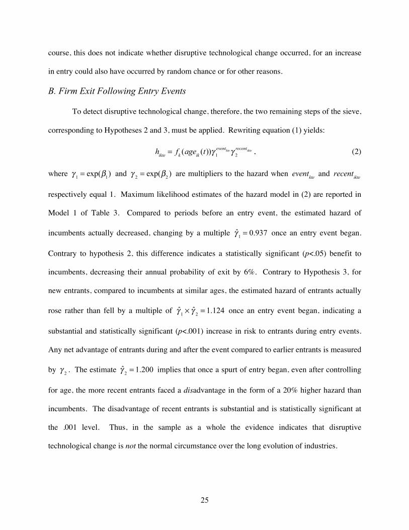
B. Firm Exit Following Entry Events
To detect disruptive technological change, therefore, the two remaining steps of the sieve,
corresponding to Hypotheses 2 and 3, must be applied. Rewriting equation (1) yields:
hikte = fk (ageik (t))γ 1eventkteγ 2
recentikte , (2)
where γ 1 = exp(β1) and γ 2 = exp(β2 ) are multipliers to the hazard when eventkte and recentikte
respectively equal 1. Maximum likelihood estimates of the hazard model in (2) are reported in
Model 1 of Table 3. Compared to periods before an entry event, the estimated hazard of
incumbents actually decreased, changing by a multiple γ̂ 1 = 0.937 once an entry event began.
Contrary to hypothesis 2, this difference indicates a statistically significant (p<.05) benefit to
incumbents, decreasing their annual probability of exit by 6%. Contrary to Hypothesis 3, for
new entrants, compared to incumbents at similar ages, the estimated hazard of entrants actually
rose rather than fell by a multiple of γ̂ 1 × γ̂ 2 = 1.124 once an entry event began, indicating a
substantial and statistically significant (p<.001) increase in risk to entrants during entry events.
Any net advantage of entrants during and after the event compared to earlier entrants is measured
by γ 2 . The estimate γ̂ 2 = 1.200 implies that once a spurt of entry began, even after controlling
for age, the more recent entrants faced a disadvantage in the form of a 20% higher hazard than
incumbents. The disadvantage of recent entrants is substantial and is statistically significant at
the .001 level. Thus, in the sample as a whole the evidence indicates that disruptive
technological change is not the normal circumstance over the long evolution of industries.

26
C. Possible Changes Over Time
Perhaps this finding is merely because in the earlier to mid 1900s complacent
competition gave incumbents a lasting advantage, while disruptive technological change has
become important later in the 1900s. Indeed, this would coincide with the finding that
competitive entry into new markets has accelerated over the course of the 1900s (Agarwal and
Gort, 2001). To test the idea of a rise in the occurrence of disruptive technological change, the
coefficients already included in the model were interacted with calendar time. The resulting
model is
hikte = fk (agei (t))exp[β1eventkte + β2recentikte + β3t × eventkte + β4t × recentikte] , (3)
where t represents mean-adjusted calendar time, the year minus 1947.7. Rewriting equation (3)
yields the same model specified in terms of multipliers to the hazard:
hikte = fk (agei (t))γ 1eventkteγ 2
recentikteγ 3t×eventkteγ 4
t× recentikte ,
where γ 1 and γ 2 are as defined for equation (2), and γ 3 and γ 4 specify the multiple by which
the effects of an entry event and of recent entry increase (decrease) for each year after (before)
the mean of 1947.7.
Estimates of the model are reported in the columns of Table 3 labeled Model 2. The
estimate γ̂ 1 = 0.957 confirms that in the mean year of the sample, entry events were associated
with a slightly decreased hazard for incumbents relative to earlier years. However, also in the
mean year, the estimate γ̂ 1 × γ̂ 2 = 1.138 (p<.001) implies that recent entrants experienced an
even higher growth in the hazard of exit. The estimate γ̂ 2 = 1.189 implies that late entrants
faced a disadvantage in terms of a hazard 1.189 times that of incumbents even after controlling
for firm age, a noteworthy and statistically significant disadvantage.

27
The estimates γ̂ 3 = 1.007 and γ̂ 4 = 0.994 indicate the changing impacts of entry events
on the hazard. For incumbent firms the rise in the hazard associated with entry events did
increase over time. For each year after 1947.7, the rise in the hazard associated with entry events
increased by a multiple of γ̂ 3 = 1.007 per year. Thus by the last year of any products in the
sample, 1992, the estimated impact of entry events on the hazard of incumbents was to multiply
the hazard by γ 1 × γ 31992−1947.7 = 1.318 . This effect of time on incumbent hazards during entry
events is statistically significant at the .001 level. For recent entrants, the time trend was one of
decreasing disadvantage associated with late entry. For recent entrants during entry events, the
hazard in 1992 was estimated to be higher by a multiple of
γ 1 × γ 31992−1947.7 × γ 2 × γ 4
1992−1947.7 = 1.216 . After an entry event had commenced, by 1992 the
hazard of recent entrants was an estimated multiple of γ 2 × γ 41992−1947.7 = 0.923 compared to that
of incumbents. The gradual decline in the recent-entrant disadvantage associated with entry
events is statistically significant at the p<.001 level.
One interpretation of these findings is that disruptive technological change was
overpowered by forces causing early entrant advantage in the early 1900s through about the
1970s, but thereafter disruptive technological change conveyed an advantage to recent entrants.
An alternative interpretation, however, is that some of the new entrants in the 1970s and later
were successful multinational firms that had already produced in other nations and then
proceeded to set up manufacturing facilities in the United States. This would explain why
suddenly new businesses entered existing markets in substantial numbers and were successful
while previous late entrants had failed.

28
D. Sensitivity Analyses
Sensitivity analyses were used to probe the robustness of the findings. One might be
concerned lest the results be biased in favor of events in a few industries with large sample sizes
relative to the others. To deal with this possibility, Table 4 reports estimates like Models 1 and 2
using the same Cox proportional hazard models, but with each industry’s contribution to the
likelihood function weighted in inverse proportion to the number of firm-years of data available
for that industry. The results are similar to those reported earlier, confirming that the findings
apparently are not biased by occurrences in industries with large sample sizes.
E. Findings by Industry and Time
The above analyses showed that on average periods with entry events coincided with
more successful performance of incumbent producers than of entrants, exactly opposite the
pattern expected of disruptive technological change. However, in specific industries and for
specific entry events it could still be the case that disruptive effects occurred. Hence independent
Cox hazard regressions were carried out separately for each of the entry events identified in
section 5A. Only firms that entered before or during each entry event are included in the data for
the statistical analysis. Table 5 reports estimates of γ 1 , γ 2 , and γ 1 × γ 2 from equation (2) for
each of the entry events.
For each event, the years of relatively high entry are indicated. The columns labeled γ̂ 1 ,
γ̂ 2 , and γ̂ 1γ̂ 2 indicate the estimated multipliers to the hazard of exit, along with corresponding
indications of statistical significance. Preceding the estimates, a check mark without parentheses
indicates an event for which the estimated coefficients are consistent with disruptive
technological change having provided an advantage to new entrants and a disadvantage to

29
incumbents. That is, a check mark appears whenever γ̂ 1 > 1 and γ̂ 1γ̂ 2 < 1. A pair of check
marks without parentheses would indicate that these patterns are both at least marginally
statistically significant (p<.10), although this never occurs.
If there were in fact no relation between a firm’s entry time and its hazard of exit, one
should observe γ̂ 1 > 1 and γ̂ 1γ̂ 2 < 1 for approximately 1 in 4 entry events.17 Given 60 entry
events, we should thus expect 15 of the events in Table 5 to bear check marks even if disruptive
technological change never occurs. In fact only 10 events, noticeably (but not significantly18)
less than the number expected by random chance, are estimated to have experienced increased
hazard of incumbent producers and decreased hazard of entrants relative to incumbents at similar
ages.
Some readers may worry about exogenous shifts in the hazard, so a weaker test examines
whether disruptive technological change provided a relative advantage to new entrants, γ 2 < 1 ,
which would be consistent with disruption even if hazard rates of all firms changed exogenously
during the period following the entry event. Preceding the estimates in Table 5, a check mark
inside parentheses indicates an event for which the estimated coefficients are consistent with this
weaker test, and a pair of check marks inside parentheses indicates at least marginally statistical
significance (p<.10). Using this criterion, 24 of 60 entry events have γ̂ 2 < 1 , whereas random
chance would suggest that half of all events, or 30, would have γ̂ 2 < 1 (again the difference is
17 This null hypothesis therefore presumes independent changes in incumbent versus entrant exit rates.
18 If each check mark occurs with 1 in 4 probability, there is an 8.6% chance of 10 or fewer check marks
plus a 9.2% chance of 20 or more check marks, so p=.178 (two-sided).

30
statistically insignificant).19 Two events are marginally statistically significant at the p<.10 level,
whereas by random chance one would expect 2.4 such marginally significant events. The two
events are typewriters for new entrants in 1970-77 and phonograph records in 1972-79.
F. Typewriters and Phonograph Records
For typewriters, the entry event in 1970-1977 corresponds to the advent of word
processing typewriters, and this trend is apparent in the industry’s entrants. Firms like Trendata,
Redactron Corp. (soon bought by Burroughs), Qume Corp., and Wang Laboratories, involved
primarily with computers or computer printers, developed word processing units after
International Business Machines’ (IBM’s) 1964 development of a typewriter with magnetic
recording, plus its 1969 Magnetic Card Selectric Typewriter (Creative Strategies International,
1977, 1981). IBM, the leader in developing the new technology, was a longtime industry player.
IBM entered the typewriter market in 1933 when it purchased a ten-year-old electric typewriter
venture, Electromatic Typewriters, and built its product into the first particularly high-selling
electric typewriter (Beeching, 1974).
Electric typewriters would bring revolution to the industry, but the revolution was slow to
arrive. An electric typewriter was patented by 1855, and as early as 1902 Blickensderfer’s
“Blick Electric” typewriter included a “typeball” mechanism in an electric typewriter. IBM took
advantage of its R&D, manufacturing, marketing, and distribution strengths in office machinery,
and by 1940 had about a 10% market share, behind four firms each with about 20% share
(Engler, 1969, p. 49). IBM’s share grew to 16% of the values of shipments in 1950 (FTC, 1972,
p. 257), and among office (non-portable) typewriters it had reached 50% by the mid-1960s and
19 If each check mark occurs with 1 in 2 probability, there is 7.8% chance of 24 or fewer check marks plus
a 7.8% chance of 36 or more check marks, so p=.155 (two-tailed).

31
69% by 1969 (FTC, 1973, p. 22316). Its share growth was aided by an innovative typeball
design in 1961, echoing the early Blickensderfer approach. Thus its successful development of
electric typewriters eventually helped IBM to take over the market, over a century after the debut
of the electric typewriter, and just before the computer revolution would undo the typewriter’s
role.
Electric typewriters, word processors, and computers thus seem genuine radical changes
that caused disruption in the industry, but the processes of their disruption seem to confirm the
cross-industry statistical findings’ admonition. Electric typewriters were an oft-used technology
that became dominant over a century after its debut. Word processors indeed spurred entry in
the 1970s, but during the remaining period with available data, exit of incumbents was most
likely spurred by IBM’s continuing development of electric typewriters. Even by 1979 word
processors made up only $264 million in sales relative to $1,004 million for other electric office
typewriters (Creative Strategies International, 1981, p. 31), and thus seem unlikely to have been
the major cause of exit, albeit that word processor entrants fared well in their growing market
niche. What word processors heralded was the more important transition to the computer, a
transition initially dominated by IBM.
For phonograph records, composed of recording firms, the 1972-1979 period of increased
entry, with a corresponding increase in incumbent exit rate, does not seem to have corresponded
to any missed innovation on the part of incumbents. Possibly the increased exit rate of
incumbents from 1972 on may have stemmed from incumbents’ highly competitive pursuit of

32
market segmentation as an improved strategy to control the industry (Tschmuck, 2006, pp. 133-
147).20 However, disruptive change in the phonograph record industry did occur earlier.
Tschmuck (2006) concludes that the music recording industry experienced two periods of
radical innovation. Both radical innovations involved radio broadcasting. In the 1920s, major
record producers refused to cooperate with the new radio broadcasting medium, and lost market
share while new labels used radio to promote musical genres like jazz, blues, and country that
had largely been ignored as “race” and “hillbilly” music by established firms.21 One major firm,
Columbia Graphophone, filed for insolvency and was bought by its British subsidiary.
In the 1950s, a rapidly growing number of radio stations turned to replayed records as a
means to cheaply serve fragmented markets.22 Fortunately for them, fragile shellac records were
replaced starting in 1948 with unbreakable vinyl media, which finally could be shipped
nationwide by businesses without specialized distribution networks (Peterson, 1990, pp. 100-
101). Vinyl records made it easy for new labels to ship records widely and hence for stations
readily to create new market niches, including rock music which became wildly popular despite
major firms’ unwillingness to record this emerging genre (which again stemmed substantially
20 The increased incumbent exit rate coincided with a more than doubling of the U.S. industry’s value of
sales from 1972 to 1978 (Gronow and Saunio, 1998, p. 137).
21 Electrical recording also was initially eschewed by major firms (Tschmuck, 2006).
22 The Federal Communications Commission restricted urban markets to three to five licensed radio
stations in the 1930s, and the major radio networks removed their objections to further licensing when it
seemed that television would make radio outmoded and the broadcasters largely turned to television
(Peterson, 1990, pp. 101-102).

33
from “race” music).23 The industry’s top four firms in 1948 controlled 81% of top-ten hits, but
by 1959 their share fell to just 34% as numerous new entrants broke into the industry (Peterson
and Berger, 1975). New businesses like Warner, MCA, and PolyGram became majors along
with previous industry leaders such as RCA, CBS, and EMI, and the new majors consolidated
the industry again and established operating methods that successfully absorbed new forms of
music (Tschmuck, 2006, pp. 137-147).24
The 1920s and 1950s revolutions, major as they were, did not quite fit the model of
strong technological disruptions assessed here. They led to substantial entry of new firms, but
they pitted small firms (new and old) against majors rather than new firms against established
firms. Also, their results seem to have been rearrangements of market share rather than exit of
the incumbent majors. Thus, while phonograph records did experience some forms of disruptive
technological change, it was not the simple “strong” sort that involved entry of new firms and
increased incumbent exit.
VI. Conclusion
This study investigated the frequency of strongly disruptive technological change, i.e.,
technological disruptions that cause some entry and incumbent exit, as a means to understand
typical competitive forces facing new ventures. In the 47 U.S. manufacturing industries studied
over periods of many decades, disruptive technological change apparently was rare or
23 Tape recorders, stemming from the German Magnetophone perfected during World War II, also
simplified small labels’ recording (Tschmuck, 2006, p. 99).
24 One company formed as late as 1962, A&M Records, held by 1973 a 7.7% share of the top 100 charts
(Vlahakis, 1975, p. 175); it would be bought by PolyGram in 1989.
34
nonexistent. Following times when unusual amounts of entry occurred, new firms rarely
experienced lower exit rates than those of incumbents even after controlling for firm age in the
industry. Indeed, in aggregate statistical analyses, incumbent producers at the times of these
surges of entry had relatively low chance of exit, while new entrants had relatively high chance
of exit, after controlling for firm age. Moreover, in statistical analyses carried out independently
for each product and each occurrence when there was a surge of entry, the number of
occurrences in which the probability of exit rose for incumbents and fell for new entrants was
about as high as one would expect due to random fluctuations in firm exit. Out of 2,221
combined years in the 47 industries, zero to a handful of strong disruptions seem to have
occurred.
The findings show that strongly competitively disruptive technological change must be
rare. If disruptive technological change is occurring more frequently in existing industries, then
it must be occurring either without a surge of entry or by affecting market shares only in
relatively minor ways so that incumbents do not become unprofitable and exit as a result. The
discussion of the typewriter industry provides a case in which just a single entrant managed to
use disruptive technology to take over much of the market, and the takeover took about four
decades. The literature on disruptive technological change is often interpreted as suggesting that
successful disruption is important and widespread. The truth seems to be that while important, it
also almost never occurs through a wave of entry followed by sufficient competition to force out
some incumbents within existing product industries.
Four qualifications of this finding deserve to be made. First, the findings stem from only
47 industries, all manufacturing industries, and it is possible that a somewhat higher frequency of
disruptive technological change could occur among all manufacturing industries or among non-

35
manufacturing industries. Second, the industry definitions used leave open the possibility that
disruptive change occurs more frequently when a new product category begins – for example the
advent of transistors which led to the downfall of vacuum tubes. Third, the analysis treats
independent divisions established by incumbents along with incumbents, and therefore addresses
how often incumbents lose their business to new entrants, which differs from Christensen’s
(2006) emphasis that incumbents may be forced to set up divisions in order to survive
technological transitions. Fourth, only within-industry disruptions have been analyzed, not
disruptions that coincide with the creation of entire new product industries.
A series of studies mentioned earlier has shown that many of the industries studied here
in fact experienced rapid technological change. That technological change, however, was of a
kind that reinforced the advantages of incumbent producers, rather than triggering disruptions
and allowing new firms to replace old firms. Hence it appears that competence-enhancing
technological change is far more frequent than competence-destroying technological change.
The phenomenon of disruptive technological change is extremely important when it occurs, and
a topic deserving much further study, but apparently, compared to the perceptions that many
researchers have held, strong technology-driven disruptions in industry competition are
surprisingly rare.
The literature on technological change and industries has pointed out two roads to riches:
entry into industries newly created by the creation of a technology, and entry into existing
industries with a new technology that gives an advantage over the old. It appears that the first
road is a well-trodden way to commercial profit, while the latter road is rarely to be found.

36
References
Adner, Ron, When Are Technologies Disruptive? A Demand-Based View of the Emergence of
Competition. Strategic Management Journal 23, 2002, pp. 667-688.
Adner, Ron, and Peter Zemsky. 2005. Disruptive technologies and the emergence of
competition. RAND Journal of Economics 36(2) 229-254.
Agarwal, Rajshree. 1988. Evolutionary Trends of Industry Variables. International Journal of
Industrial Organization 16(4) 511-525.
Agarwal, R., M. Gort. 2001. First mover advantage and the speed of competitive entry, 1887-
1986. Journal of Law and Economics 44(1) 161-178.
Anderson, P., M. Tushman. 1990. Technological discontinuities and dominant designs: A
cyclical model of technological change. Admin. Sci. Quart. 35(4) 604-633.
Anderson, P., M. Tushman. 2001. Organizational environments and industry exit: The effects of
uncertainty, munificence and complexity. Industrial and Corporate Change 10(3) 675-711.
Argyres, Nicholas, and Anita M. McGahan. 2002. An Interview with Michael Porter. Academy
of Management Executive 16(2) 43-52.
Arrow, Kenneth. 1962. Economic Welfare and the Allocation of Resources for Invention. In The
Rate and Direction of Inventive Activity. Universities-National Bureau of Economic Research:
Princeton University Press, 1962, pp. 609-625.
Audretsch, D. B. 1991. New-firm survival and the technological regime. Review of Economics
and Statistics 73(3) 441-450.
Bai, Jushan, and Pierre Perron. 1998. Estimating and testing linear models with multiple
structural changes. Econometrica 66(1) 47-78.

37
Bai, Jushan, and Pierre Perron. 2003. Computation and analysis of multiple structural change
models. Journal of Applied Econometrics 18(1) 1-22.
Beeching, Wilfred A. Century of the Typewriter. New York: St. Martin’s Press, 1974.
Christensen, C. M. 1997. The Innovator’s Dilemma. Harvard Business School Press, Boston,
MA.
Christensen, C.M. 2006. The ongoing process of building a theory of disruption. Journal of
Product Innovation Management 23 39-55.
Christensen, C. M., R. S. Rosenbloom. 1995. Explaining the attacker’s advantage: Technological
paradigms, organizational dynamics, and the value network. Res. Policy 24(2) 233-257.
Christensen, C. M., F. F. Suárez, and J. M. Utterback, 1998. Strategies for survival in fast-
changing industries, Management Sci. 44(12-2) S-207-220.
Cooper, Arnold C., and Dan Schendel, Strategic Responses to Technological Threats. Business
Horizons, February 1976, pp. 61-69.
Creative Strategies International. Word Processing Typewriter Industry. San Jose, CA: Creative
Strategies International, 1977.
Creative Strategies International. Intelligent and Office Electric Typewriters. San Jose, CA:
Creative Strategies International, 1981.
Engler, George Nichols. The Typewriter Industry: The Impact of a Significant Technological
Innovation. PhD dissertation, University of California at Los Angeles, 1969.
Federal Trade Commission (FTC). 1958. Economic Report on Antibiotics Manufacture.
Washington, D.C.: U.S. Government Printing Office.

38
Federal Trade Commission (FTC). 1972. Statistical Report [on] Value of Shipments Data by
Product Class for the 1,000 Largest Manufacturing Companies of 1950. Washington, D.C.:
U.S. Government Printing Office.
Federal Trade Commission (FTC). 1973. “D.8778, Litton Industries, Inc. Final Order, March 14,
1973,” in Trade Regulation Reporter, New York: Commerce Clearing House, Inc., circa pp.
22316-22317.
Foster, Richard N. Innovation: The Attacker’s Advantage. New York: Summit Books, 1986.
Gans, Joshua S., David H. Hsu, and Scott Stern. When Does Start-up Innovation Spur the Gale
of Creative Destruction. RAND Journal of Economics 33(4), 2002, pp. 571-586.
Gilbert, Richard and David Newberry. Preemptive Patenting and the Persistence of Monopoly.
American Economic Review 72 (3: June), 1982, pp. 514-526.
Gort, M., S. Klepper. 1982. Time paths in the diffusion of product innovations. Economic
Journal 92(367) 630-653.
Gronow, Pekka, and Ilpo Saunio. 1998. An International History of the Recording Industry.
London: Cassell.
Henderson, R. M., 1993. Underinvestment and incompetence as responses to radical innovation:
Evidence from the photolithographic alignment equipment industry. RAND Journal of
Economics 24(2) 248-270.
Henderson, R M., K. B. Clark. 1990. Architectural innovation: The reconfiguration of existing
product technologies and the failure of established firms. Admin. Sci. Quart. 35(1) 9-30.
King, A. A., C. L. Tucci. 2002. Incumbent entry into new market niches: The role of experience
and managerial choice in the creation of dynamic capabilities. Management Sci. 48(2) 171-
186.

39
Klepper, Steven. Firm Survival and the Evolution of Oligopoly. RAND Journal of Economics
33 (1), 2002, pp. 37-61.
Klepper, Steven, and Kenneth L. Simons. Technological Extinctions of Industrial Firms: An
Enquiry into their Nature and Causes. Industrial and Corporate Change 6, 1997, pp. 379-460.
Klepper, Steven, and Kenneth L. Simons. The Making of an Oligopoly: Firm Survival and
Technological Change in the Evolution of the U.S. Tire Industry. Journal of Political Economy
108, 2000a, pp. 728-760.
Klepper, Steven, and Kenneth L. Simons. Dominance by Birthright: Entry of Prior Radio
Producers and Competitive Ramifications in the U.S. Television Receiver Industry. Strategic
Management Journal 21 (10-11), October-November 2000b, pp. 997-1016.
Klepper, Steven, and Kenneth L. Simons. Industry Shakeouts and Technological Change.
International Journal of Industrial Organization 23 (1-2), February 2005, pp. 23-43.
Lee, Beom S., and James E. Gentle. 2009. Multiple Structural Breaks in Time Series of Count
Data: Forecasting the Number of Atlantic Hurricanes. Manuscript.
Lerner, Josh. 1997. An Empirical Exploration of a Technology Race. RAND Journal of
Economics 28(2: Summer) 228-247.
Lieberman, Marvin B., and David B. Montgomery. First-Mover (Dis)advantages: Retrospective
and Link with the Resource-Based View. Strategic Management Journal 19, 1998, pp. 1111-
1125.
Loader, Clive. 1999. Local Regression and Likelihood. New York: Springer.
Majumdar, B. A. 1982. Innovations, Product Developments, and Technology Transfers: An
Empirical Study of Dynamic Competitive Advantage, the Case of Electronic Calculators.
University Press of America, Washington, D.C.

40
McKendrick, David G., Richard F. Doner, and Stephan Haggard. 2000. From Silicon Valley to
Singapore: Location and Competitive Advantage in the Hard Disk Drive Industry. Stanford:
Stanford University Press.
Peterson, Richard A. 1990. Why 1955? Explaining the advent of rock music. Popular Music 9(1)
97-116.
Peterson, Richard A., and David G. Berger. 1975. Cycles in Symbol Production: The Case of
Popular Music. American Sociological Review 40(2) 158-173.
Reinganum, J. F. 1983. Uncertain innovation and the persistence of monopoly. American
Economic Review 73(4) 741-748.
Rothaermel, Frank T., and Charles W. L. Hill. Technological Discontinuities and
Complementary Assets: A Longitudinal Study of Industry and Firm Performance.
Organization Science 16(1), January-February 2005, pp. 52-70.
Schivardi, Fabiano, and Martin Schneider. Strategic Experimentation And Disruptive
Technological Change. Review of Economic Dynamics 11(2), April 2008, pp. 386-412.
Schnaars, S. P. 1994. Managing Imitation Strategies: How Later Entrants Seize Markets from
Pioneers. Free Press, New York.
Simons, Kenneth L. 2003. Information technology and dynamics of industry structure: The UK
IT consulting industry as a contemporary specimen. Manuscript.
Simons, Kenneth L. 2005. Product Market Characteristics and the Industry Life Cycle. Working
paper, Rensselaer Polytechnic Institute.
Smith, P. H. 1968. Wheels within Wheels: A Short History of American Motor Car
Manufacturing. Funk and Wagnalls, New York.

41
Sull, Donald N., Richard S. Tedlow, and Richard S. Rosenbloom. 1997. Managerial
commitments and technological change in the US tire industry. Industrial and Corporate
Change 6(2), pp. 461-500.
Thomas Publishing. 1905-1981. Thomas’ Register of American Manufacturers. Thomas
Publishing Co., New York.
Tripsas, Mary. 1997a. Surviving Radical Technological Change through Dynamic Capability:
Evidence from the Typesetter Industry. Industrial and Corporate Change 6(2), pp. 341-377.
Tripsas, Mary. 1997b. Unraveling the Process of Creative Destruction: Complementary Assets
and Incumbent Survival in the Typesetter Industry. Strategic Management Journal 18(Summer
special issue), pp. 119-142.
Tripsas, Mary, and Giovanni Gavetti. 2000. Capabilities, Cognition, and Inertia: Evidence from
Digital Imaging. Strategic Management Journal 21, pp. 1147-1161.
Tschmuck, Peter. 2006. Creativity and Innovation in the Music Industry. Springer, Dordrecht,
Netherlands.
Tushman, M. L., P. Anderson. 1986. Technological discontinuities and organizational
environments. Administrative Science Quarterly 31(3) 439-465.
U.S. Tariff Commission (later U.S. International Trade Commission). 1944-1992. Synthetic
Organic Chemicals. U.S. Government Printing Office, Washington, D.C.
Vlahakis, Matthew Constantine. 1975. The Condition of Entry in the Phonograph Record
Industry. PhD dissertation, Columbia University.
Warren Publishing. 1948-1991. Television Factbook (or Television and Cable Factbook).
Warren Publishing, Washington, D.C.

42
Table 1. Sample characteristics Industry Years N Entry Industry Years N Entry
adding & calc. machines 1905-79 2397 2.80 outboard motors 1909-80 1182 1.48 artificial xmas trees 1924-79 505 0.65 oxygen tents 1931-79 618 0.88 automobile tires 1905-80 5466 8.03 penicillin 1943-92 830 0.80 automobiles 1895-67 4680 9.92 phonograph records 1905-79 2079 2.59 ball-point pens 1946-79 2813 7.67 photocopy machines 1939-79 780 1.65 baseboard heaters 1947-80 616 1.24 piezo crystals 1935-79 1008 1.52 beta ray gauges 1955-79 136 0.71 polariscopes 1905-79 689 0.57 computers 1935-79 4721 13.45 radar 1945-79 4182 10.18 cryogenic tanks 1960-79 961 5.58 radio transmitters 1922-79 2450 4.26 DDT 1945-80 858 2.00 recording tapes 1951-79 1024 4.25 electric blankets 1915-79 556 0.63 rocket engines 1957-80 272 1.04 electric shavers 1936-79 529 1.14 rubber-based paint 1933-82 3201 3.86 electrocardiographs 1926-79 547 0.77 saccharin 1905-72 1027 1.18 fluorescent bulbs 1941-80 1085 1.64 shampoo 1905-79 6279 5.96 freezers 1944-80 1515 3.58 streptomycin 1946-79 209 0.55 freon compressors 1935-80 745 1.24 styrene 1937-92 1085 1.75 gas turbines 1940-79 854 2.00 telemeters 1927-79 689 1.38 guided missiles 1950-79 4078 11.62 television picture tubes 1949-71 851 3.14 gyroscopes 1913-80 1084 1.46 televisions 1948-89 1462 2.46 heat pumps 1953-79 481 2.46 transistors 1952-79 1486 5.93 jet engines 1947-79 611 1.72 typewriters 1905-79 1721 1.58 lasers 1962-79 1170 9.47 windshield wipers 1911-79 1367 2.40 microfilm readers 1939-79 494 1.80 zippers 1928-79 1968 3.49 nuclear reactors 1954-79 708 2.76
Notes: N is the number of firm-years of data. Entry is mean number of entrants per annum.

43
Table 2. Periods with high entry relative to previous (ten to) twenty years adding & calc. machines 1924-28 outboard motors 1958-64 adding & calc. machines 1949-54 oxygen tents 1949-55 artificial xmas trees 1935-39 penicillin 1983-92 artificial xmas trees 1958-66 phonograph records 1917-24 automobile tires 1916-23 phonograph records 1943-47 automobile tires 1971-80 phonograph records 1972-79 automobiles 1905-10 piezo crystals 1973-77 automobiles 1946-55 polariscopes 1916-23 computers 1945-78 polariscopes 1930-34 computers 1955-61 polariscopes 1943-58 computers 1970-75 radio transmitters 1935-79 electric blankets 1925-31 recording tapes 1970-74 electric blankets 1945-52 rubber-based paint 1946-66 electric blankets 1959-63 saccharin 1916-20 electric shavers 1972-76 saccharin 1948-52 electrocardiographs 1940-67 saccharin 1964-68 electrocardiographs 1954-65 shampoo 1924-49 electrocardiographs 1973-77 shampoo 1946-50 freon compressors 1946-50 shampoo 1973-79 freon compressors 1969-73 styrene 1955-92 gas turbines 1957-63 styrene 1974-80 gas turbines 1972-76 telemeters 1941-78 gyroscopes 1940-80 telemeters 1953-74 gyroscopes 1950-77 typewriters 1948-58 heat pumps 1975-79 typewriters 1970-77 lasers 1972-77 windshield wipers 1921-28 microfilm readers 1952-56 windshield wipers 1958-62 microfilm readers 1961-79 windshield wipers 1975-79 microfilm readers 1972-76 zippers 1938-59 outboard motors 1944-50 zippers 1972-77
Notes: The identified periods are required to be five years or longer and to have 50% higher
mean annual entry than the previous twenty years (or at least ten years if fewer than twenty have
elapsed since the first year of data). The periods are assumed to end when a period of at least
three years occurs with less than 50% higher mean annual entry.

44
Table 3. Determinants of firm hazard of exit: Cox proportional hazard models with effects of
firm age allowed to vary by industry Model 1 Model 2 mult. sig. 95% conf. int. mult. sig. 95% conf. int. Event occurred 0.937 * 0.883 0.995 0.957 0.898 1.021 Entrant after event 1.200 *** 1.121 1.284 1.189 *** 1.111 1.272 Event occurred × time 1.007 ** 1.004 1.010 Entrant after event × time 0.994 *** 0.991 0.997 Log-pseudolikelihood Firms Exits Firm-years
-41,043.878 4,996 (8,918) 4,007 (7,463)
50,652 (94,859)
-41,034.357 4,996 (8,918) 4,007 (7,463)
50,652 (94,859)
† p<.10, * p<.05, ** p<.01, *** p<.001 (two-tailed asymptotic p-values, versus multiplier of 1).
Notes: Heteroskedasticity-robust clustered variance estimates, allowing for arbitrary clustering of
random outcomes within firms, account for identical outcomes across subsamples pertaining to
different entry events in the same product. Figures in parentheses for numbers of firms, exits,
and firm-years include these identical outcomes.
Table 4. Determinants of firm hazard of exit: Weighted Cox proportional hazard models with
effects of firm age allowed to vary by industry, weighted to equalize weighted firm-years of
alternative industries Model 3 Model 4 mult. sig. 95% conf. int. mult. sig. 95% conf. int. Event occurred 0.993 0.895 1.101 1.012 0.911 1.123 Entrant after event 1.221 * 1.097 1.359 1.193 ** 1.076 1.323 Event occurred × time 1.006 ** 1.002 1.011 Entrant after event × time 1.000 0.996 1.005 Log-pseudolikelihood -32,465.631 -32,449.990 Firms Exits Firm-years
4,996 (8,918) 4,007 (7,463)
50,652 (94,859)
4,996 (8,918) 4,007 (7,463)
50,652 (94,859)
† p<.10, * p<.05, ** p<.01, *** p<.001 (two-tailed asymptotic p-values, versus multiplier of 1).
Notes: See notes to table 3. Time is relative to the weighted mean year of 1953.9.

45
Table 5. Cox hazard models for individual events Product Event Pattern γ̂ 1 γ̂ 2 γ̂ 1γ̂ 2 adding & calc. machines 1924-28 1.646 † 1.122 1.848 ** adding & calc. machines 1949-54 1.226 0.755 0.926 artificial xmas trees 1935-39 0.000 ∞ . 0.484 artificial xmas trees 1958-66 3.733 † 1.040 3.882 * automobile tires 1916-23 1.143 1.369 * 1.564 *** automobile tires 1971-80 1.485 0.606 0.899 automobiles 1905-10 0.785 1.631 *** 1.280 * automobiles 1946-55 1.148 0.632 0.725 computers 1945-78 1.337 3.023 ** 4.041 computers 1955-61 1.692 * 1.109 1.877 ** computers 1970-75 () 1.544 ** 0.762 1.176 electric blankets 1925-31 () 4.288 0.453 1.941 electric blankets 1945-52 () 0.988 0.917 0.905 electric blankets 1959-63 0.743 1.234 0.917 electric shavers 1972-76 0.738 1.615 1.192 electrocardiographs 1940-67 0.000 ∞ . 1.040 electrocardiographs 1954-65 1.010 3.429 † 3.465 * electrocardiographs 1973-77 () 3.100 * 0.427 1.324 freon compressors 1946-50 () 5.404 † 0.929 5.018 * freon compressors 1969-73 () 3.300 † 0.593 1.958 gas turbines 1957-63 0.551 2.509 † 1.382 gas turbines 1972-76 1.114 1.522 1.695 gyroscopes 1940-80 () 5.085 0.735 3.740 gyroscopes 1950-77 1.293 1.372 1.773 heat pumps 1975-79 0.322 5.268 † 1.695 lasers 1972-77 () 1.532 0.799 1.224 microfilm readers 1952-56 0.939 1.062 0.997 microfilm readers 1961-79 1.251 0.553 0.692 microfilm readers 1972-76 0.754 1.112 0.839 outboard motors 1944-50 0.445 1.907 0.848 outboard motors 1958-64 1.203 1.121 1.349 oxygen tents 1949-55 0.462 2.269 1.047 penicillin 1983-92 0.706 3.084 2.176 phonograph records 1917-24 0.413 3.020 1.247 phonograph records 1943-47 0.597 2.078 † 1.240 phonograph records 1972-79 () 1.008 0.316 † 0.318 ** piezo crystals 1973-77 1.088 0.715 0.778 polariscopes 1916-23 1.152 0.347 0.400 polariscopes 1930-34 1.305 0.000 0.000 polariscopes 1943-58 0.186 6.130 1.139 radio transmitters 1935-79 0.413 * 1.836 † 0.759 recording tapes 1970-74 () 2.116 † 0.730 1.546 rubber-based paint 1946-66 0.438 1.705 † 0.747

46
Table 5 continued. Cox hazard models for individual events Product Event Pattern γ̂ 1 γ̂ 2 γ̂ 1γ̂ 2 saccharin 1916-20 2.087 1.136 2.370 saccharin 1948-52 1.396 0.641 0.895 saccharin 1964-68 () 2.160 † 0.866 1.869 shampoo 1924-49 () 0.779 0.988 0.769 shampoo 1946-50 0.577 ** 1.139 0.658 * shampoo 1973-79 () 0.993 0.498 0.495 † styrene 1955-92 0.753 2.926 * 2.204 styrene 1974-80 1.331 1.120 1.491 telemeters 1941-78 2.650 2.130 5.645 † telemeters 1953-74 1.863 2.436 * 4.538 ** typewriters 1948-58 0.835 1.145 0.956 typewriters 1970-77 () 2.283 * 0.421 † 0.961 windshield wipers 1921-28 () 3.656 * 0.714 2.609 windshield wipers 1958-62 () 0.854 0.806 0.689 windshield wipers 1975-79 0.958 1.151 1.103 zippers 1938-59 1.713 1.132 1.939 zippers 1972-77 0.723 1.575 1.140
Notes: Pattern column indicates whether exit patterns are consistent with disruptive change:
indicates that indeed γ̂ 1 > 1 and γ̂ 1γ̂ 2 < 1 . indicates that both coefficients are statistically
significantly different from 1. A weaker test is whether γ̂ 2 < 1, which would be consistent with
disruption if the hazard rates of all firms were exogenously altered for all firms during the period
following the entry event, and events that meet only this weaker test have check marks shown in
parentheses.
† p<.10, * p<.05, ** p<.01, *** p<.001 (two-tailed asymptotic p-values, versus multiplier of 1).