TWO PROBLEMS ON HOMOGENEOUS STRUCTURES, REVISITEDcherlin/Publication/census.pdf · TWO PROBLEMS ON...

TWO PROBLEMS ON HOMOGENEOUS STRUCTURES,

REVISITED

GREGORY CHERLIN

Abstract. We take up Peter Cameron’s problem of the classification of count-ably infinite graphs which are homogeneous as metric spaces in the graph met-ric [Cam98], working toward an explicit catalog of “known” examples on theone hand, and an investigation of the cases which occur as exceptional casesfrom the perspective of the catalog.

We begin with a presentation of Fraısse’s theory of amalgamation classesand the classification of homogeneous structures, with emphasis on the caseof homogeneous metric spaces, from the discovery of the Urysohn space to theconnection with topological dynamics developed in [KPT05]. We then turn toa discussion of the case of metrically homogeneous graphs.

We also take this opportunity to revisit another old chestnut from thetheory of homogeneous structures, namely the problem of approximating thegeneric triangle free graph by finite graphs. Very little is known about this,but it is possible to rephrase the problem in somewhat more explicit geometricterms. And in that form one can raise questions that seem appropriate fordesign theorists, as well as some questions that involve structures small enoughto be explored computationally.

Introduction

A metric space M is said to be homogeneous if every isometry between finitesubsets of M is induced by an isometry taking M onto itself. An interesting andearly example is the Urysohn space U [Ury25, Ury27] found in the summer of1924, the last product of Urysohn’s short but intensely productive life. While theproblem of Frechet that prompted this construction concerned universality ratherthan homogeneity, Urysohn took particular notice of this homogeneity property inhis initial letter to Hausdorff [Hus08], a point repeated in much the same terms inthe posthumous announcement [Ury25]. We will discuss this in §2 below.

From the point of view of Fraısse’s later theory of amalgamation classes [Fra54],the essential point is that finite metric spaces can be amalgamated: if M1,M2 arefinite metric spaces whose metrics agree on their common part M0 = M1∩M2, thenthere is a metric on M1 ∪M2 extending the given metrics; and more particularly,the same applies if we limit ourselves to metric spaces with a rational valued metric.

Fraısse’s theory facilitates the construction of infinite homogeneous structuresof all sorts, which are then universal in various categories, and is often used tothat effect. This gives a construction of Rado’s universal graph [Rad64], as well

Date: June 20, 2010.1991 Mathematics Subject Classification. Primary 03C10; Secondary 03C13, 03C15, 05B,

20B22, 20B27.Key words and phrases. homogeneous structure, permutation group, finite model property,

model theory, amalgamation, topological dynamics, extreme amenability, Ramsey theory.Supported by NSF Grant DMS 0100794.

1

2 GREGORY CHERLIN

as Henson’s universal Kn-free graphs [Hen71], and uncountably many quite similarhomogeneous directed graphs [Hen72, Henson]; a variant of the same constructionalso yields uncountably many homogeneous nilpotent groups and commutative rings[CSW]. More subtly, the theory of amalgamation classes can also be used to classifyhomogeneous structures of various types: homogeneous graphs [LW80], homoge-neous directed graphs [Sch79, Lac84, Che88, Che98], the finite and the imprimitiveinfinite graphs with two edge colors [Che99], the homogeneous partial orders witha vertex coloring by countably many colors [TT08], and even homogeneous permu-tations [Cam02].

There is a remarkable 3-way connection linking the theory of amalgamationclasses, structural Ramsey theory, and topological dynamics, developed in [KPT05].In this setting the Urysohn space appears as one of the natural examples, but morefamiliar combinatorial structures come in on an equal footing.

The Fraısse theory, and the connection with topological dynamics, will be re-viewed in §3.

In §4 we will discuss how Fraısse’s theory has been used to obtain classificationsof all the homogeneous structures in some limited classes.

Every connected graph is a metric space in the graph metric, and Peter Cameronraised the question of the classification of the graphs which are homogeneous asmetric spaces [Cam98]. Such graphs are referred to as metrically homogeneous ordistance homogeneous. This condition is much sharper than the condition of dis-tance transitivity which is familiar in finite graph theory; the complete classificationof the finite distance transitive graphs is much advanced and actively pursued. Heraised that issue in the context of his “census” of the very rich variety of countablyinfinite distance transitive graphs, and our title echoes his. We aim for a morecomplete catalog of the known graphs meeting this very strong condition, as wellas a demonstration that at the margins this catalog is reasonably complete. Thisremains a work in progress: the catalog is still not in satisfactory form, as we shallsee.

We also take this occasion to look at another problem connected with homoge-neous structures, namely the question of the finite model property for the universalhomogeneous triangle free graph [Che93], one of Henson’s homogeneous graphs[Hen71]. The problem is the construction, for each k, of a finite triangle free graphwith the properties that (i) any maximal independent set of vertices has order atleast k; and (ii) for any set A of k independent vertices, and any subset B of A,there is a vertex adjacent to all vertices of B and no vertices of A\B—or, of course,a proof that for some k there is no such finite graph. Some examples are known forthe case k = 3, notably the Higman-Sims graph (as observed by Simon Thomas),as well as an infinite family constructed by Michael Albert, again with k = 3. Westill have no example with k = 4, and we will suggest that the lack of variety amongthe known examples for k = 3 is worth further attention in its own right, and raisessome problems that seem relatively accessible.

This lack of variety in the case k = 3 leads to some problems that seem relativelyaccessible. We will review the situation in §4. One arrives at a class of combinatorialgeometries whose constraints do not appear to be overly restrictive, but for whichwe have remarkably few examples. Some of the best examples to date come fromstrongly regular triangle free graphs, but there are also more elementary examples,in infinite families. The supply is rather limited, and to get an example with k = 4

TWO PROBLEMS ON HOMOGENEOUS STRUCTURES, REVISITED 3

would require, in particular, having much more satisfactory examples for k = 3. Sowe will make this point explicit. What we have in mind is somewhat in the spiritof [Bon09]. We will also show that the case k = 4 cannot be handled using stronglyregular graphs. Peter Cameron mentioned to me many years ago that bounds inthe theory of strongly regular graphs should limit the possibilities for some suchvalue of k. My impression is that the case k = 4 is something of a squeaker, andI found the explicit formulas in [Big09] helpful in dealing with this case. I don’tsuppose, in the present state of knowledge, one can expect to bound the size ofa strongly regular graph satisfying our conditions for k = 3, as this seems to bebound up with the central problems of the field. But perhaps the experts can dosomething with that as well.

The theory of homogeneous structures has many other aspects that we will nottouch upon, many connected with the study of the automorphism groups of homo-geneous structures, e.g. the small index property and reconstruction of structuresfrom their automorphism groups [DNT86, HHLS93, KT01, Rub94, Tr09], grouptheoretic issues [Tru85, Tru03, Tr09], and the classification of reducts of homoge-neous structures [Tho91, Tho91], which is tied up with structural Ramsey theory.There is also an elaborate theory due to Lachlan treating stable homogeneous rela-tional structures systematically as limits of finite structures, and by the same tokengiving a very general analysis of the finite case

The subject of homogeneity falls under the much broader heading of “oligomor-phic permutation groups”, that is the study of infinite permutation groups havingonly finitely many orbits on n-tuples for each n. As the underlying set is infinite,this property has the flavor of a very strong transitivity condition, and leads to avery rich theory [Cam09, Cam96].

4 GREGORY CHERLIN

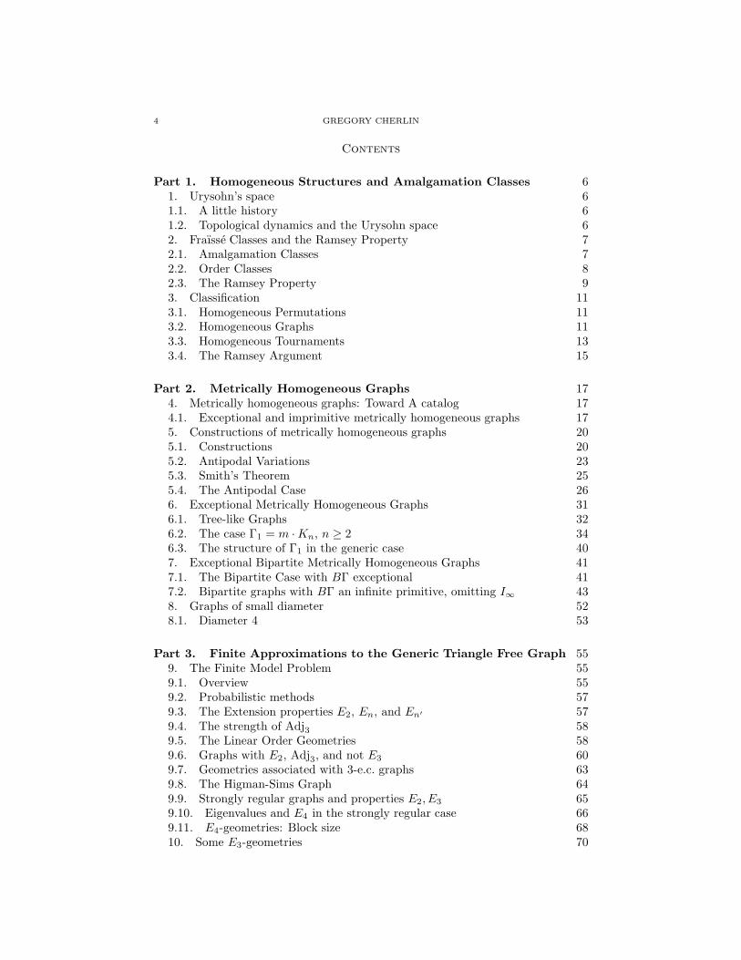
Contents

Part 1. Homogeneous Structures and Amalgamation Classes 61. Urysohn’s space 61.1. A little history 61.2. Topological dynamics and the Urysohn space 62. Fraısse Classes and the Ramsey Property 72.1. Amalgamation Classes 72.2. Order Classes 82.3. The Ramsey Property 93. Classification 113.1. Homogeneous Permutations 113.2. Homogeneous Graphs 113.3. Homogeneous Tournaments 133.4. The Ramsey Argument 15

Part 2. Metrically Homogeneous Graphs 174. Metrically homogeneous graphs: Toward A catalog 174.1. Exceptional and imprimitive metrically homogeneous graphs 175. Constructions of metrically homogeneous graphs 205.1. Constructions 205.2. Antipodal Variations 235.3. Smith’s Theorem 255.4. The Antipodal Case 266. Exceptional Metrically Homogeneous Graphs 316.1. Tree-like Graphs 326.2. The case Γ1 = m ·Kn, n ≥ 2 346.3. The structure of Γ1 in the generic case 407. Exceptional Bipartite Metrically Homogeneous Graphs 417.1. The Bipartite Case with BΓ exceptional 417.2. Bipartite graphs with BΓ an infinite primitive, omitting I∞ 438. Graphs of small diameter 528.1. Diameter 4 53

Part 3. Finite Approximations to the Generic Triangle Free Graph 559. The Finite Model Problem 559.1. Overview 559.2. Probabilistic methods 579.3. The Extension properties E2, En, and En′ 579.4. The strength of Adj3 589.5. The Linear Order Geometries 589.6. Graphs with E2, Adj3, and not E3 609.7. Geometries associated with 3-e.c. graphs 639.8. The Higman-Sims Graph 649.9. Strongly regular graphs and properties E2, E3 659.10. Eigenvalues and E4 in the strongly regular case 669.11. E4-geometries: Block size 6810. Some E3-geometries 70


10.1. Albert geometries 7010.2. Another series of E3-geometries 7310.3. E3-Geometries of order at most 7 7510.4. A small non-Albert geometry 7711. Appendix: Amalgamation Classes (Data from [Che98]) 77References 78

6 GREGORY CHERLIN

Part 1. Homogeneous Structures and Amalgamation Classes

1. Urysohn’s space

1.1. A little history. A special number of Topology and its Applications (vol. 155)contains the proceedings of a conference on the Urysohn space (Beer-Sheva, 2006).A detailed account of the circumstances surrounding the discovery of that space,shortly before a swimming accident took Urysohn’s life off the coast of Brittany, canbe found in the first section of [Hus08], which we largely follow here. There is alsoan account of Urysohn’s last days in [GK09], which provides additional context.

Urysohn completed his habilitation in 1921, and his well known contributionsto topology were carried out in the brief interval between that habilitation and hisfatal accident on August 17th, 1924. Frechet raised the question of the existenceof a universal complete separable metric space (one into which any other shouldembed isometrically) in an article published in the American Journal of Mathe-matics in 1925 with a date of submission given as August 21, 1924. Frechet hadcommunicated his question to Aleksandrov and Urysohn some time before that,and an announcement of a solution is contained in a letter from Aleksandrov andUrysohn to Hausdorff dated August 3, 1924, a letter to which Hausdorff replied indetail on August 11. The letter from Aleksandrov and Urysohn is quoted in theoriginal German in [Hus08]. In that letter, the announcement of the construction ofa universal complete separable metric space is followed immediately by the remark:“. . . and in addition [it] satisfies a quite powerful condition of homogeneity: thelatter being, that it is possible to map the whole space onto itself (isometrically)so as to carry an arbitrary finite set M into an equally arbitrary set M1, congruentto the set M .” The letter goes on to note that this pair of conditions, univer-sality together with homogeneity, actually characterizes the space constructed upto isometry. This comment on the property of homogeneity is highlighted in verysimilar terms in the published announcement [Ury25].

Urysohn’s construction proceeds in two steps. He first constructs a space U0, nowcalled the rational Urysohn space, which is universal in the category of countablemetric spaces with rational-valued metric. This space is constructed as a limit offinite rational-valued metric spaces, and Urysohn takes its completion U as thesolution to Frechet’s problem.

It is the rational Urysohn space which fits neatly into the general frameworklater devised by Fraısse [Fra54]. A countable structure is called homogeneous ifany isomorphism between finitely generated substructures is induced by an auto-morphism of M . If we construe metric spaces as structures in which the metricdefines a weighted complete graph, with the metric giving the weights, then finitelygenerated substructures are just finite subsets with the inherited metric, and iso-morphism is isometry. Other examples of homogeneity arise naturally in algebra,such as vector spaces (which may carry forms—symplectic, orthogonal, or unitary),or algebraically closed fields. We will mainly be interested in relational systems,that is combinatorial structures in which “f.g. substructure” simply means “finitesubset, with the induced structure.” But Fraısse’s general theory, to which we turnin the next section, does allow for the presence of functions.

1.2. Topological dynamics and the Urysohn space. The Urysohn space, orrather its group of isometries, turns up in topological dynamics as an example of thephenomenon of extreme amenability. A topological group is said to be extremely


amenable if any continuous action on a compact space has a fixed point. Theisometry group of Urysohn space is shown to be extremely amenable in [Pes02],and subsequently the general theory of [KPT05] showed that the isometry group ofthe ordered rational Urysohn space (defined in the next section) is also extremelyamenable. The general theory of [KPT05] requires Fraısse’s setup, but we quoteone of the main results in advance:

Theorem 1. [KPT05, Theorem 2] The extremely amenable closed subgroups of theinfinite symmetric group Sym∞ are exactly the groups of the form Aut(F ), whereF is the Fraısse limit of a Fraısse order class with the Ramsey property.

We turn now to the Fraısse theory.

2. Fraısse Classes and the Ramsey Property

2.1. Amalgamation Classes. It is not hard to show that any two countable ho-mogeneous structures of a given type will be isomorphic if and only if they havethe same isomorphism types of f.g. substructures. This uses a “back-and-forth”constructions, as in the usual proof of that any two countable dense linear ordersare isomorphic, which is indeed a particular instance. In view of this uniqueness,it is natural to look for a characterization of countable homogeneous structuresdirectly in terms of the associated class Sub(M) of f.g. structures embedding intoM . Fraısse identified the relevant properties:

I. Sub(M) is hereditary (closed downward, and under isomorphism): in otherwords, if A is in the class, then any f.g. structure isomorphic with a sub-structure of A is in the class;

II. There are only countably many isomorphism types represented in Sub(M);III. Sub(M) has the joint embedding and amalgamation properties: if A1, A2 are

f.g. substructures in the class, and A0 embeds into A1, A2 isomorphically viaembeddings f1, f2, then there is a structure A in the class with embeddingsA1, A2 → A, completing the diagram

The joint embedding property is the case in which M0 is empty, which should betreated as a distinct condition if one does not allow empty structures.

A key point is that amalgamation follows from homogeneity: taking A0 to bea subset of A1, and embedded into A2, apply an automorphism of the ambientstructure to move the image of A0 in A2 back to A0, and A2 to some isomorphicstructure A′

2 containing A0; then the structure generated by A1 ∪ A2 will serve asan amalgam.

Conversely, if A is a class of structures with properties (I − III), then thereis a countable homogeneous structure M , unique up to isomorphism, for whichSub(M) = A. This homogeneous structure M is called the Fraısse limit of theclass A. Thus with A taken as the class of finite linear orders, the Fraısse limit is

8 GREGORY CHERLIN

isomorphic to the rational order; with A the class of all finite graphs, the Fraısselimit is Rado’s universal graph [Rad64]; and with A the class of finite rational-valued metric spaces, after checking amalgamation, we take the Fraısse limit to getthe rational Urysohn space. The computation that checks amalgamation can befound in Urysohn’s own construction, though not phrased as such.

So we see that Fraısse’s theory is at least a ready source of “new” homogeneousstructures, and we now give a few more examples in the same vein. Starting withthe class of all partial orders, we obtain the “generic” countable partial order (tocall it merely “dense,” as in the linear case, would be to understate its properties).Or starting with the class of finite triangle free graphs, we get the “generic” trian-gle free graph, and similarly for any n the generic Kn-free graph will be obtained[Hen71]. The amalgamation procedure here is simply graph theoretical union, andthe special role of the complete graphs here is due to their indecomposability withrespect to this amalgamation procedure: a complete graph which embeds into thegraph theoretical union of two graphs (with no additional edges permitted) mustembed into one of the two. The generalization to the case of directed graphs isimmediate: amalgamating via the graph theoretical union, the indecomposable di-rected graphs are the tournaments. So we associate with any set of tournamentsT the Fraısse class of finite directed graphs omitting T —i.e., with no directed sub-graph isomorphic to one in T . The corresponding Fraısse limits are the genericT -free graphs considered by Henson [Hen72]. The richness of the construction isconfirmed by showing that 2ℵ0 directed graphs arise in this way, because of the ex-istence of an infinite antichain in the class of finite tournaments, that is an infiniteset X of finite tournaments, which are pairwise incomparable under embedding, sothat each subset of X gives rise to a different Fraısse limit. A suitable construc-tion of such an antichain is given by Henson [Hen72]. A parallel construction inthe category of commutative rings provides, correspondingly, uncountably manyhomogeneous commutative rings [CSW].

The structure of the infinite antichains of finite tournaments has been investi-gated further, but has not been fully elucidated. Any such antichain lies over onewhich is minimal in an appropriate sense, and after some close analysis by Latka[Lat94, La03, La02] a general finiteness theorem emerged [CL00] to the effect thatfor any fixed k, there is a finite set of minimal antichains which will serve as univer-sal witnesses for any collection of finite tournaments determined by k constraints(forbidden tournaments) which allows an infinite antichain. This means that when-ever such an antichain is present, one of the given antichains is also present, up toa finite difference. But there is still no known a priori bound for the number ofantichains required, as a function of k. Even the question as to whether the numberof antichains needed is bounded by a computable function of k remains open.

In the terminology of [KPT05], the notion of Fraısse class is taken to incorporatea further condition of local finiteness, meaning that all f.g. structures are finite. Thismay be viewed as a strengthening of condition (II). This convention is in force, inparticular, in the statement of Theorem 1, which we now elucidate further.

2.2. Order Classes. The Fraısse classes that occur in the theorem of Kechris-Pestov-Todorcevic above are order classes: this means that the structures consid-ered are equipped with a distinguished relation < representing a linear order. Thusin this theorem nothing is said about graphs, directed graphs, or metric spaces,but rather their ordered counterparts: ordered graphs, ordered directed graphs,


ordered metric spaces. In particular the ordered rational Urysohn space is, by defi-nition, the homogeneous ordered rational valued metric space delivered by Fraısse’stheory. As there is no connection between the order and the metric the necessaryamalgamation may be carried out separately in both categories.

In the most straightforward, and most common, applications of the Fraısse theorythere is often some notion of “free amalgamation” in use. In the case of orderclasses amalgamation cannot be entirely canonical, as some “symmetry breaking” isinevitable. But there are also finite homogeneous structures—such as the pentagongraph, or 5-cycle—for which the theory of amalgamation classes is not illuminating,and the amalgamation procedure consists largely of the forced identification ofpoints.

When one passes from the construction of examples to their systematic classi-fication, there is typically some separation between the determination of more orless sporadic examples, and the remaining cases described naturally by the Fraıssetheory. Such a classification has only been carried out in a few cases, and perhapsa more nuanced picture will appear eventually.

We will say something more about how the theory of [KPT05] applies in theabsence of order, but first we complete the interpretation of Theorem 1 by discussingthe second key property required.

2.3. The Ramsey Property. The ordinary Ramsey theorem is expressed in Hun-garian notation by the symbolism:

∀k,m, n ∃N : N → (n)mk

meaning that for given k,m, n, there is N so that: for any coloring of increasingm-tuples from A = {1, . . . , N} by k colors, there is a subset B of cardinality nwhich is monochromatic with respect to the coloring.

Structural Ramsey theory deals with a locally finite hereditary class A of finitestructures of fixed type, which on specialization to the case of the class L of finitelinear orders will degenerate to the usual Ramsey theory. In general, given twostructures A,B in A, write

(

BA

)

for the class of induced substructures of B isomor-

phic to A. This gives(

Nn

)

an appropriate meaning if A = L, namely increasingsequences of length n from an ordered set of size N .

We may then use the Hungarian notation

M → (B)Ak

to mean that whenever we have a coloring of of(

MA

)

by k colors, there is a copy of

B inside M which is monochromatic with respect to the induced coloring of(

BA

)

.And the Ramsey property will be:

∀A,B ∈ A∀k ∃M ∈ A : M → (B)Ak

So the Ramsey property for L is the usual finite Ramsey theorem.Ramsey theory for Fraısse classes is a subtle matter, but a highly developed

one. In [HN05] it is shown that the Ramsey property implies the amalgamationproperty, by a direct argument. What one would really like to classify are the Fraısseclasses with the Ramsey property, but according to [HN05] the most promisingroute toward that is via classification of amalgamation classes first, and then theidentification of the Ramsey classes.

10 GREGORY CHERLIN

For unordered graphs, the only instances of the Ramsey property that holdare those for which the subgraphs being colored are complete graphs Kn, or theircomplements [NR75b]. But the collection of finite ordered graphs does have theRamsey property [NR77a, NR77b, AH78].

To illustrate the need for an ordering, consider colorings of the graph A =K1 +K2, a graph on 3 vertices with one edge, and let B = 2 · K2 be the disjointsum of two complete graphs of order 2. If we order B in any way, we may color thecopies of A in B by three colors according to the relative position of the isolatedvertex of A, with respect to the other two vertices, namely before, after, or betweenthem. Then B, with this coloring, cannot be monochromatic. Thus we can neverhave a graph G satisfying G → (B)A3 , since given such a graph G we would firstorder G, then define a coloring of copies of A in G as above, using this order, andthere could be no monochromatic copy of B.

The significance of the ordered rational Urysohn space only emerged in [KPT05],and the appropriate structural Ramsey theorem was proved “on demand” by Nesetril[Nes07].

At this point, we have collected all the notions needed for Theorem 1. Beforewe leave this subject, we note that the theory of [KPT05] also exhibits a directconnection between the more classical examples of the Fraısse theory (lacking abuilt-in order). The following is a fragment of Theorem 5 of [KPT05].

Theorem 2. Let G be the automorphism group of one of the following countablestructures M :

(1) The random graph;(2) The generic Kn-free graph, n ≥ 2;(3) The rational Urysohn space.

Let L be the space of all linear orderings of M , with its compact topology as a closedsubset of 2M×M . Then under the natural action of G on L, L is the universalminimal compact flow for G.

The minimality here means that there is no proper closed invariant subspace;and the universality means that this is the largest such minimal flow (projecting onto any other). Again, Theorem 2 has an abstract formulation in terms of Fraıssetheory [KPT05]. The following is a special case.

Theorem 3 ([KPT05, Theorem 4]). Let A be a (locally finite) Fraısse class andlet A+ be the class of ordered structures (K,<) with K ∈ A. Suppose that A+ is aFraısse class with the order property and the Ramsey property. Let M be the Fraısselimit of A, G = Aut(M), and L the space of linear orderings of M , equipped withthe compact topology inherited by inclusion into 2M×M . Then under the naturalaction of G on L, the space L is the universal minimal compact flow for G.

Here one has in mind the case in which amalgamation in A does not requireany identification of vertices (strong amalgamation); then A+ is certainly an amal-gamation class. The order property is the following additional condition: givenA ∈ A, there is B ∈ A such that under any ordering on A, and any ordering on B,there is some order preserving isomorphic embedding of A into B. This is againa property which must be verified when needed, and is known in the cases cited.To see an example where the order property does not hold, consider the class A offinite equivalence relations. Any equivalence relation B may be ordered so that itsclasses are intervals; thus the order property fails.


We turn next to the problem of classifying homogeneous structures of particulartypes. Here again the Fraısse theory can be helpful.

3. Classification

The homogeneous structures of certain types have been completely classified,notably homogeneous graphs [LW80], homogeneous tournaments [Lac84], homo-geneous tournaments with a coloring by finitely many colors and homogeneousdirected graphs [Che88], homogeneous partial orders with a coloring by countablymany colors [TT08], and homogeneous permutations [Cam02]: this last is a lessfamiliar notion, that we will enlarge upon. There is also work on the classificationof homogeneous 3-hypergraphs [LT95, AL95], and on graphs with two colors ofedges [Lac86, Che99], the latter covering only the finite and imprimitive cases: thisuncovers some sporadic examples, but the main problem remain untouched in thisclass.

3.1. Homogeneous Permutations. Cameron observed that permutations havea natural interpretation as structures, and that when one adopts that point ofview the model theoretic notion of embedding is the appropriate one. A finitepermutation may naturally be viewed as a finite structure consisting of two linearorderings. This is equivalent to a pair of bijections between the structure and theset {1, . . . , n}, n being the cardinality, and thus to a permutation. In this setting,an embedding of one permutation into another is an occurrence in the second of apermutation pattern corresponding to the first, so that this formalism meshes nicelywith the subject of permutations omitting specified patterns.

By a very direct analysis, Cameron showed that there are just 6 homogeneouspermutations, in this sense, up to isomorphism: the trivial permutation of order1, the identify permutation of Q or its reversal, the class corresponding to the lex-icographic order on Q × Q, where the second order agrees with the first in onecoordinate and reverses the first in the other coordinate, and the generic permu-tation (corresponding to the class of all finite permutations). The existence of thegeneric permutation is immediate by the Fraısse theory.

As amalgamations of linear orders are tightly constrained, the classification ofthe amalgamation classes of permutations is quite direct. Cameron also observesthat it would be natural also to generalize from structures with two linear orders toan arbitrary finite number, but I do know of any further progress on this question.

3.2. Homogeneous Graphs. This is the case that really launched the classifica-tion project. The classification of homogeneous graphs by Lachlan and Woodrowinvolves an ingenious inductive setup couched directly in terms of amalgamationclasses of finite graphs. We will need the results of that classification later, whendiscussing distance homogeneous graphs. Indeed, homogeneous graphs are just thediameter two (or less) case of distance homogeneous graphs. Furthermore, in anydistance homogeneous graph, the graph induced on the neighbors of a point is ahomogeneous graph, and one may consider each of the possibilities individually.

We begin with a catalog of the homogeneous graphs. We use the notation Kn

for a complete graph of order n, allowing n = ∞, meaning ℵ0 in this context. Wewrite In for the complement of Kn, that is (an independent set of vertices of ordern, and m · Kn for the disjoint sum of m copies of Kn, again allowing m and n to

12 GREGORY CHERLIN

become infinite. Bearing in mind that the complement of a homogeneous graph isagain a homogeneous graph, we arrange the list as follows.

I. Degenerate cases, Kn or In; here, one of the available 2-types is not actuallyrealized, so these are actually structures for a simpler language.

II. Imprimitive homogeneous graphs, m · Kn and their complements, wherem,n ≥ 2. The complement of m · Kn is complete n-partite with parts ofconstant size.

III. Primitive, nondegenerate, homogeneous finite graphs (highly exceptional):the pentagon or 5-cycle C5, and a graph on 9-points which may be describedas the line graph of the complete bipartite graphK3,3, or the graph theoreticsquare of K3.

IV. Primitive, nondegenerate, infinite homogeneous graphs, with which the clas-sification is primarily concerned: Henson’s generic graphs omitting Kn, andtheir complements, generic omitting In, as well as the generic or randomgraph Γ∞ (Rado’s graph) corresponding to the class of all finite graphs.

In this setting there is no difficulty identifying the degenerate and imprimitiveexamples, and little difficulty in identifying the remaining finite ones by an inductiveanalysis. Since the class of homogeneous graphs is closed under complementation,the whole classification comes down to the following result.

Theorem 4 ([LW80, Theorem 2′, paraphrased]). Let Γ be a homogeneous non-degenerate primitive graph containing an infinite independent set, as well as thecomplete graph Kn. Then Γ contains every finite graph not containing a copy ofKn+1.

Let us see that this completes the classification in the infinite, primitive, nonde-generate case. As the graph Γ under consideration is infinite, by Ramsey’s theoremit contains either K∞ or I∞, and passing to the complement if necessary, we maysuppose the latter. So if Kn embeds in Γ and Kn+1 does not, then Theorem 4says that Γ is the corresponding Henson graph, while if Kn embeds in Γ for all n,Theorem 4 then says that it is the Rado graph.

The method of proof is by induction on the order N of the finite graph G whichwe wish to embed in Γ. The difficulty is that on cursory inspection, Theorem4 does not at all lend itself to such an inductive proof. Lachlan and Woodrowshow that as sometimes happens in such cases, a stronger statement may be provedby induction. Their strengthening is on the extravagant side, and involves someadditional technicalities, but it arises naturally from the failure of the the first tryat an inductive argument. So let us first see what difficulties appear in a directattack.

Let G be a graph of orderN , not containingKn+1, and let Γ be the homogeneousgraph under consideration. We aim to show that G embeds in Γ, proceeding byinduction on N . Pick a vertex v of G. If v is isolated, or if v is adjacent tothe remaining vertices of G, we will need some special argument (even more solater, once we strengthen our inductive claim). For example, if v is adjacent to theremaining vertices of G, then we have an easy case: we identify v with any vertexof Γ, we consider the graph Γ1 on the vertices adjacent to v in Γ, and after verifyingthat Γ1 inherits all hypotheses on Γ (with n replaced by n − 1) we can concludedirectly by induction on n. If the vertex v is isolated, the argument will be lessimmediate, but still quite manageable.


Turning now to the main case, when the vertex v has both a neighbor and a non-neighbor in G, matters are considerably less simple. Let G0 be the graph inducedon the other vertices of G, and let a, b be vertices of G0 chosen with a adjacent tov, and b not. At this point, we must build an amalgamation diagram which forcesa copy of G into Γ, and we hope to get the factors of the diagram by induction onN , which of course does not quite work. It goes like this.

Let A be the graph obtained from G by deleting v and a, and let B be the graphobtained from G by deleting v and b. Let H be the disjoint sum A+B of A and B,and form two graphs H1 = H0 ∪ {u} and H2 ∪ {c}, with edge relations as follows.The vertex u plays the role of v, and is therefore related to A and B as v is in G.The vertex c plays a more ambiguous role, as a or b, and is related to A as a is,and to B as b is.

Suppose for the moment that copies of H1, H2 occur in Γ. Then so does anamalgam H1 ∪H2 over H0, and in that amalgam either u is joined to c, which maythen play the role of a, with the help of A, or else u is not joined to c, and then cmay play the role of b, with the help of B. In either case, a copy of G is forced intoΓ.

What may be said about the structure of H1 and H2? These are certainly toolarge to be embedded into Γ by induction, but they have a simple structure: H1

is the free amalgam of A ∪ {a} with B ∪ {b} under the identification of a with b,and H2 is constructed similarly, over u. Here each factor (e.g., A ∪ {a}, A ∪ {b} inthe case of H1) embeds into Γ by induction, but we need also the sum of the twofactors over a common vertex. This leads to the following definitions.

Definition 3.1.

1. A pointed graph (G, v) is a graph G with a distinguished vertex v.2. The pointed sum of two pointed graphs (G, v) and (H,w) is the graph obtained

from the disjoint sum G+H by identifying the base points.3. Let A(n) be the set of finite graphs belonging to every amalgamation class

which contains Kn, I∞, the path of order 3, and its complement (the last twoeliminate imprimitive cases).

4. Let A∗(n) be the set of finite graphs G such that for any vertex v of G, andany pointed graph (H,w) with H ∈ A(n), the pointed sum (G, v) + (H,w) belongsto A(n).

Notice that A∗(n) is contained in A for trivial reasons, simply taking for (H,w)the pointed graph of order 1. Now we can state the desired strengthening of The-orem 2′.

Theorem 5 ([LW80, Lemma 6]). For any n, if G is a finite graph omitting Kn+1,then G belongs to A∗(n).

With this definition, the desired inductive proof actually goes through. Admit-tedly the special cases encountered in our first run above become more substantialthe second time around. As a result, this version of the main theorem will bepreceded by 5 other preparatory lemmas required to support the final induction.However the process of chasing one’s tail comes to an end at this point.

3.3. Homogeneous Tournaments. In Lachlan’s classification of the homoge-neous tournaments [Lac84] two new ideas occur, which later turned out to besufficient to carry out the full classification of the homogeneous directed graphs

14 GREGORY CHERLIN

[Che98], with suitable orchestration. A byproduct of that later work was a moreefficient organization of the case of tournaments, given in [Che88]. The main ideaintroduced at this stage was a certain use of Ramsey’s theorem that we will describein full. The second idea arises naturally at a later stage as one works through theimplications of the first; it involves an enlargement of the setting beyond tourna-ments, where much as in the case of the Lachlan/Woodrow argument, the pointis to find an inductive framework large enough to carry through an argument thatleads somewhat beyond the initial context of homogeneous tournaments.

It turns out that there are only 5 homogeneous tournaments, four of them of aspecial type which are easily classified, and the last one fully generic. The wholedifficulty comes in the characterization of this last tournament as the only ho-mogeneous tournament of general type, in fact the only one containing a specifictournament of order 4 called [T1, C3]. In this notation, T1 is the tournament oforder 1, C3 is a 3-cycle, and [T1, C3] is the tournament consisting of a vertex (T1)dominating a copy of C3. So the analog of Theorem 2′ of [LW80] is the following.

Theorem 6 ([Lac84]). Let T be a countable homogeneous tournament containinga tournament isomorphic with [T1, C3]. Then every finite tournament embeds intoT .

We now give the classification of the homogeneous tournaments explicitly, andindicate the reduction of that classification to Theorem 6.

A local order is a tournament with the property that for any vertex v, the tour-naments induced on the sets v+ = {u : v → u} and v− = {u : u → v} are bothtransitive (i.e., given by linear orders). Equivalently, these are the tournaments notembedding [T1, C3] or its dual [C3, T1]. There is a simple structure theory for thelocal orders, which we will not go into here. But the result is that there are exactlyfour homogeneous local orders, two of them finite: the trivial one of order 1, andthe 3-cycle C3. The infinite homogeneous local orders are the rational order (Q, <)and a very similar generic local order, which can be realized equally concretely.

Now a tournament T which does not contain a copy of [T1, C3] can easily beshown to be of the form [S,L] where S is a local order whose vertices all dominatea linear order L; here S or L may be empty. Indeed, if T is homogeneous, one of thetwo must be empty, and in particular T is a local order. Thus if the homogeneoustournament T contains a copy of [T1, C3] then it contains a copy of [C3, T1] as well,and it remains only to prove Theorem 6.

At this point, the following interesting technical notion comes into the picture.If A is an amalgamation class, let A∗ be the set of finite tournaments T such thatevery tournament T ∗ of the following form belongs to A: T ∗ = T ∪ L, L is linear,and any pattern of edges between T and L is permitted. Theorem 6 is equivalentto the following rococo variation.

Theorem 7. If A is an amalgamation class containing [T1, C3], then A∗ is anamalgamation class containing [T1, C3].

That A∗ is an amalgamation class is simply an exercise in the definitions, butworth working through to see why the definition of A∗ takes the particular formthat it does (because linear orders have strong amalgamation). The deduction ofTheorem 6 from Theorem 7 is also immediate. Assuming Theorem 7, we argueby induction on N = |T | that T belongs to any amalgamation class A containing


[T1, C3]. Take any vertex v of T and let T0 be the tournament induced on the re-maining vertices. By induction, T0 belongs to every amalgamation class containing[T1, C3], in particular T0 ∈ A∗. Since T is the extension of T0 by a single vertex,and since a single vertex constitutes a linear tournament, then from T0 ∈ A∗ wederive T ∈ A, and we are done.

Note the progress which has been made. In Theorem 6 we consider arbitrarytournaments; in Theorem 7 we consider only linear extensions of [T1, C3]. Now afurther reduction comes in, and eventually the statement to be proved reduces to afinite number of specific instances of Theorem 6 which can be proved individually.But we have not yet encountered the leading idea of the argument, which comes inat the next step.

3.4. The Ramsey Argument. We introduce another class closely connected withA∗.

Definition 3.2.

1. For tournaments A,B we define the composition A[B] as usual as the tour-nament derived from A by replacing each vertex of A by a copy of B, with edgesdetermined within each copy of B as in B, and between each copy of B, as in A.The composition of two tournaments is a tournament.

2. If T is any tournament, a stack of copies of T is a composition L[T ].3. If A is an amalgamation class of finite tournaments, let A∗∗ be the set of

tournaments T such that every tournament T ∗ of the following form belongs to A:T ∗ = L[T ] ∪ {v} is the extension of some stack of copies of T by one more vertex.

The crucial point here is the following.

Fact 3.3. Let A be an amalgamation class of finite tournaments, and T a finitetournament in A∗∗. Then T belongs to A∗.

We will not give the argument in detail here. It is a direct application of theRamsey theorem, given explicitly in [Lac84] and again in [Che88, Che98]. The ideais that one may amalgamate a large number of one point extensions of a long stackof copies of T so that in any amalgam, the additional points contain a long lineartournament, and one of the copies of T occurring in the stack will hook up withthat linear tournament in any previously prescribed fashion desired.

This leads to our third, and nearly final, version of the main theorem.

Theorem 8. Let A be an amalgamation class of finite tournaments. Then C3

belongs to A∗∗.

Notice that a stack of copies of [T1, C3] embeds in a longer stack of copies of C3,so that Theorem 8 immediately implies that the same result for [T1, C3]. Since wealready saw that A∗∗ ⊆ A∗, Theorem 8 implies Theorem 7. In view of the verysimple structure of a stack of copies of T , we are almost ready to prove this laststatement by induction on the length of the stack. Unfortunately the additionalvertex v occurring in T ∗ = L[T ] ∪ {v} complicates matters, and leads to a furtherreformulation of the statement.

At this point, it is convenient to return from the language of amalgamationclasses to the language of structures. So let the given amalgamation class corre-spond to the homogeneous tournament T, and let T = L[C3] ∪ {v} be a 1-pointextension of a finite stack of 3-cycles. Theorem 8 says that T embeds into T. Itwill be simpler to strengthen the statement slightly, as follows.

16 GREGORY CHERLIN

Let a be an arbitrary vertex in T, and consider T1 = a+ and T2 = a− separately.We claim that T embeds into T with L[C3] embedding into T1, and with the vertexv going into T2. This now sets us up for an inductive argument in which we considera single 3-cycle C in T1, and the parts T′

1 and T′2 defined relative to C as follows:

T′1 consists of the vertices of T1 dominated by the three vertices of C, and T′

2

consists of the vertices v′ which relate to C as the specified vertex v does. Whatremains at this point is to clarify what we know, initially, about T1 and T2, and toshow that these properties are inherited by T′

1 and T′2 (in particular, T′

2 should benonempty!). This then allows an inductive argument to run smoothly.

At this point we have traded in the tournament T for a richer structure (T1,T2)consisting of a tournament with a distinguished partition into two sets. The homo-geneity of T will give us the homogeneity of (T1,T2) in its expanded language. Suchstructures will be called 2-tournaments, and the particular class of 2-tournamentsarising here will be called ample tournaments. The main inductive step in theproof of Theorem 8 will be the claim that an ample tournament (T1,T2) gives riseto an ample tournament (T′

1,T′2) if we fix a 3-cycle in T1 and pass to the subsets

considered above.We do not wish at all to dwell on this last part. The main steps in the proof are

the reduction to Theorem 8, and then the realization that we should step beyondthe class of homogeneous tournaments to the class of homogeneous 2-tournaments,to find a setting which is appropriately closed under the construction correspondingto the inductive step of the argument. This then leaves us concerned only aboutthe base of the induction, which reduces to a small number of specific claims abouttournaments of order not exceeding 6. Once the problem is finitized, it can besettled by explicit amalgamation arguments.

Lachlan’s Ramsey theoretic argument functions much the same way in the con-text of directed graphs as it does for tournaments, and comes more into its ownthere, as it is not a foregone conclusion that Ramsey’s theorem will necessarily pro-duce a linear order; but it will produce something, and modifying the definition ofA∗ to allow for this additional element of vagueness, things proceed much as theydid before.

In [Che98] there is also a treatment of the case of homogeneous graphs using theideas of [Lac84] in place of the methods of [LW80]. This cannot be said to be asimplification, having roughly the complexity of the original proof, but it is a viablealternative, and the proof of the classification of homogeneous directed graphs ismore or less a combination of the ideas of the tournament classification with theideas which appear in a treatment of homogeneous graphs by this second method.

This ends our general survey of the general theory of amalgamation classes itsapplication to classification results. It is not clear how much further those ideascan be taken. The proofs are long and ultimately computational even when thefinal classifications have a reasonably simple form, and the subject has not gonemuch beyond this point. There may be some scope for further applications ofthese ideas in the case of metrically homogeneous graphs, but this still remainsto be seen. So we have looked more toward the construction of generic types ofmetrically homogeneous graphs on the one hand, and the classification of the moreexceptional types, on the other, for which such techniques are not needed. So as faras the present exposition is concerned, we will not be returning to these methods.But their availability should be borne in mind.


In the remaining sections we will focus on the two open problems mentionedalready in the introduction.

Part 2. Metrically Homogeneous Graphs

4. Metrically homogeneous graphs: Toward A catalog

Any connected graph may be considered as a metric space under the graph met-ric, and if the associated metric space is homogeneous then the graph is said to bemetrically homogeneous [Cam98]), or (by analogy with distance transitivity) dis-tance homogeneous. Cameron asked whether this class of graphs can be completelyclassified, and gave some examples of constructions via the Fraısse theory of amal-gamation classes in [Cam98]. He also noted that for graphs of diameter at most2, the metric structure is the same as the graph structure, so that the problembecomes the classification of homogeneous graphs, whose solution by Lachlan andWoodrow was discussed in §3. Also noteworthy in this regard is the classificationby Macpherson of the infinite, locally finite distance transitive graphs [Mph82],and the treatment of the finite case in [Cam80]. Further examples are found intables given at the end of [Che98]. These tables present all the primitive metri-cally homogeneous graphs of diameter 3 or 4 which can be defined by forbiddinga set of triangles, excluding those of diameter 3 in which none of the forbiddentriangles involve the distance 2 (in which case one automatically has an amalga-mation class). Those tables require some decoding for our purposes: they makeno explicit mention of metric spaces, but simply deal with homogeneous structuresdetermined by constraints on triples—many, but not all, of these can be construedas metric spaces. So we will translate this information into our present context.While preparing this report, I learned of ongoing work in [AMP10], which shedsconsiderable light on the case of diameter 3.

For any homogeneous metric space Γ, and for any i up to the diameter of Γ, theset Γi of points at distance i from a fixed vertex of Γ will again be a homogeneousmetric space. But if Γ is a metrically homogeneous graph, the distance 1 may notoccur in the metric space Γi, in which case the induced metric will not come fromthe induced graph. This is a major complication for any inductive analysis of themetrically homogeneous graphs, and suggests that in order to treat this problem itmay eventually be necessary to embed it in an even larger classification problem.

On the other hand, when distance 1 does occur in Γi, then Γi can be viewed as ametrically homogeneous graph (not necessarily connected). There is a small pointto be checked here, which is covered in [Cam98]. In particular for small values ofi, Γi will have smaller diameter than Γ, and if the metric is in fact a graph metricthen that graph can be supposed known, inductively. For larger values of i theinduced graph will be no more complicated than Γ, a point which may sometimesbe exploited, in a more delicate way.

4.1. Exceptional and imprimitive metrically homogeneous graphs. In set-ting out our catalog, we begin by noticing two classes of metrically homogeneousgraphs which deserve special attention. On the one hand, we have the imprimi-tive ones: these have a nontrivial equivalence relation definable without parameters(equivalently, invariant under the full automorphism group). In the finite distancetransitive case, these are described by Smith’s Theorem [Smi71]; this theorem is an

18 GREGORY CHERLIN

effective tool for reduction to the primitive case when the graph is finite, and alsoto a significant degree when the graph is infinite.

An explicit version of Smith’s theorem, laying out the various subcases whichnaturally arise, is given in [AH06]. Leaving aside the case of n-cycles, which areimprimitive whenever n is composite, there are only two ways in which a connecteddistance transitive graph can be imprimitive: it may be bipartite, or it may be“antipodal”. This means that the diameter δ is finite and the relation “d(x, y) ∈{0, δ} is an equivalence relation. Of course, the graph may be both bipartite andantipodal. Smith’s theorem says a good deal more than this, and we will elaboratewhen we explore the imprimitive metrically homogeneous case.

The other special class of metrically homogeneous graphs worthy of particularattention arises from the Lachlan/Woodrow classification. If Γ is a metrically ho-mogeneous graph, Γ1 is a metrically homogeneous graph with respect to the edgerelation “d(x, y) = 1” (though Γ1 may be an independent set). The cases whicharise naturally in connection with Fraısse style constructions are the following: Γi

is an independent set; Γ1 is generic omitting Kn for some n; Γ1 is the Rado graph(fully generic). Any other possibility will be considered exceptional: that is Γ1

finite, or infinite imprimitive, or generic omitting an independent set In for somen.

These exceptional graphs may be explicitly classified, and this classification willgive the point of departure for our catalog. The following result, to be proved in§6, refers to some specific constructions that will be described subsequently.

Theorem 9. Let Γ be a connected metrically homogeneous graph. Then one of thefollowing occurs.

(1) Γ has diameter at most 2, and is homogeneous as a graph (cf. §3):(2) Γ has degree 2, and is an n-cycle for some n.(3) Γ1 is finite or imprimitive, and Γ is one of the following.

(a) Antipodal of diameter 3, and the result of doubling C5, E(K3,3), or afinite independent set (Theorem 15);

(b) A tree-like graph Tr,s as described by Macpherson [Mph82].(4) Γ is of generic type, meaning that Γ1 is one of the following three types:

(a) An infinite independent set; and furthermore, for u ∈ Γ2, the set ofneighbors of u in Γ1 is infinite;

(b) Generic omitting a complete graph Kn, for some n ≥ 3 finite;(c) Homogeneous universal (Rado’s graph).

Given the Lachlan/Woodrow theorem, observe that the locally finite case iscovered by the result of Cameron in the finite case, and the result of Macpherson inthe infinite case. We will indicate direct proofs below, but it should be noted thatthe analyses of Cameron and Macpherson use less than metric homogeneity. Theproof of Macpherson’s theorem in full generality is far more subtle than the specialcase that concerns us here. We claim in addition that no new cases arise with Γ1

infinite and imprimitive, or generic omitting In for some n.Next in order, we consider the infinite bipartite case. If Γ is a connected bipar-

tite metrically homogeneous graph, then one denotes by BΓ the metric structureinduced on either “half” of Γ, rescaled by a factor of 1/2; in particular BΓ becomesa graph with edge relation “d(x, y) = 2”. This gives us another metrically homoge-neous graph, of half the diameter (rounded down) of Γ. In particular up through


diameter 5, the associated graph BΓ is an ordinary homogeneous graph, found inthe Lachlan/Woodrow classification.

By definition any infinite bipartite metrically homogeneous graph falls on the“generic” side of our initial classification, but the same need not apply to BΓ. Thenext result says that apart from some explicitly classifiable examples, which areeither trees or have diameter at most 5, our graph BΓ is of generic type, and evenhas BΓ1 homogeneous universal (i.e., BΓ1 is Rado’s graph). In particular, BΓ isnot itself bipartite.

Theorem 10. Let Γ be a connected, bipartite, and metrically homogeneous graph,of diameter at least 3, and degree at least 3. Then one of the following occurs,writing BΓ1 for (BΓ)1.

(1) Γ is a tree;(2) Γ has diameter 3, and Γ is either the complement of a perfect matching, or

a generic bipartite graph;(3) Γ has diameter 4, BΓ ∼= K∞[I2], and Γ is a double cover of a generic

bipartite graph, described in Lemma 7.2 below.(4) Γ has diameter 4, and BΓ1 is generic omitting an independent set of order

n+ 1, for some n ≥ 2. With n fixed, Γ is determined up to isomorphism.(5) Γ has diameter 5 and is antipodal; BΓ1 is generic omitting an independent

set of order 3. Γ is determined up to isomorphism.(6) BΓ1 is a homogeneous universal graph.

Each of these possibilities occurs.

In the antipodal case, our analysis deviates considerably from the finite case. Inthe finite case, one works with the broader class of distance transitive graphs (oreven more broadly than that). Then there is a natural quotient operation whichgives a distance transitive graph structure on the equivalence classes for the antipo-dality relation: we join two classes by an edge if there are representatives joinedby an edge. Unfortunately, this does not work well in the metrically homogeneoussetting, as we shall see. On the other hand, we will derive the following strongconstraint.

Proposition 4.1. Let Γ be a connected metrically homogeneous and antipodalgraph, of diameter δ ≥ 3. Then for each vertex u ∈ Γ, there is a unique vertexu′ ∈ Γ at distance δ from u, and we have the law

d(u, v) = δ − d(u′, v)

for u, v ∈ Γ. In particular, the map u 7→ u′ is an automorphism of Γ.

This does not give us a direct reduction of the classification to the primitivecase, but it does suggest that the antipodal, and not bipartite, case may be broadlysimilar to the primitive case.

We have still to consider graphs which are both antipodal and bipartite. In thecase of odd diameter, that is covered by the following.

Theorem 11. Let Γ be a metrically homogeneous graph of odd diameter 2d + 1which is both antipodal and bipartite. Then BΓ is a primitive infinite metricallyhomogeneous graph with the following properties:

(1) BΓ has diameter d;(2) No triangle in BΓ has perimeter greater than 2d+ 1;

20 GREGORY CHERLIN

(3) BΓ is not antipodal.

For any metrically homogeneous graph G with these three properties, there is anantipodal bipartite graph of diameter 2d+ 1 with BΓ ∼= G, and G determines Γ upto isomorphism.

We do not know anything similar in the case of even diameter. In this case, BΓwill again be antipodal, but not bipartite. We do not have a general description ofthe class of graphs occurring as BΓ, or information about the extent to which BΓdetermines Γ.

At this point, we have looked at the various special cases which naturally arise,and we have seen a number of issues that need further exploration. We turn nowto a discussion of the known constructions that produce graphs of generic type,including some which are bipartite, antipodal, or both. Two of our constructionsare already familiar from the study of universal graphs with forbidden subgraphs,see [KMP88, Kom99].

5. Constructions of metrically homogeneous graphs

We are concerned here with the use of Fraı sse constructions to produce metri-cally homogeneous graphs of generic type, including some bipartite and antipodalcases.

5.1. Constructions. We begin by setting out three examples of amalgamationclasses of finite integral metric spaces, with our usual proviso that the distancesoccurring exhaust an interval [0, δ] in N, so that the corresponding homogeneousstructure can be construed as a graph with the graph metric. In general, we expectthe typical amalgamation class to be an intersection of these three types.

Fix δ with 3 ≤ δ ≤ ∞, and let Mδ be the collection of all finite integral-valuedmetric spaces of diameter at most δ. With δ fixed, we will consider forbiddenstructures of the following two types:

• A triangle is a metric space with 3 points; its perimeter is the sum of thethree distances involved. The type of a triangle is the triple (i, j, k) ofdistances between pairs of points, taken in any order.

• A (1, δ)-space is a metric space in which all distances are equal to 1 or δ,where if δ = ∞ this means that all distances are equal to 1.

We then define the following classes of finite metric spaces contained in Mδ.

(1) For 1 ≤ K1 ≤ K2 ≤ δ or K1 = ∞, K2 = 0, let AδK1,K2

be the class of

X ∈ Mδ such that for any triangle of type (i, j, k) embedding in X , if theperimeter P = i+ j + k is odd then it satisfies:

P ≥ 2K1 + 1 and 2P ≤ 2K2 +min(i, j, k)

(2) For any C0, C1 ≥ 2δ + 1 with C0 odd and C1 even, let BδC0,C1

be the class

of X ∈ Mδ such that for any triangle of type (i, j, k) embedding in X , ifthe perimeter P = i+ j + k has parity ǫ (i.e. P ∼= ǫ mod 2 and ǫ = 0 or 1)then

P < Cǫ

(3) For any set S of (1, δ)-spaces, let CδS be the class of X ∈ Mδ such that no

space in S embeds isometrically into X .


(4) With δ,K1,K2, C0, C1, S as above let AδK1,K2;C0,C1;S

be the intersection

AδK1,K2

∩ BδC0,C1

∩ CδS

Certain values of theKi and Ci will result in the exclusion of various (1, δ)-spacesand as a rule we would include in S only the minimal constraints not alreadyexcluded on that basis, but there is no real harm in allowing some redundancy.Many but not all of the classes Aδ

K1,K2;C0,C1;Swill be amalgamation classes. To

describe the precise conditions needed on the paramters, it is convenient to takethe pair C0, C1 in increasing order, so we set

C = min(C0, C1), C′ = max(C0, C1)

In laying out the precise conditions needed we take the case K1 = ∞ as a specialcase, and for K1 < ∞ we consider further whether or not C ≤ 2δ +K1; and somefurther conditions are necessary when C′ > C + 1. So we distinguish three cases,with some further subdivision.

Theorem 12. Let δ ≥ 3, 1 ≤ K1 ≤ K2 ≤ δ, 2δ + 1 ≤ C0, C1 ≤ 3δ + 2 withC0 even and C1 odd, and S a set of (1, δ)-spaces occurring in Aδ

K1,K2;C0,C1. Let

C = min(C0, C1) and C′ = max(C0, C1). Then the class

AδK1,K2;C0,C1;S

is an amalgamation class if and only if one of the following sets of conditions issatisfied.

(1) K1 = ∞:

K2 = 0, C1 = 2δ + 1, and S is a set of δ-cliques.

(2) K1 < ∞ and C ≤ 2δ +K1:

C = 2K1 + 2K2 + 1, K1 +K2 ≥ δ, and K1 + 2K2 ≤ 2δ − 1If C′ > C + 1 then K1 = K2 and 3K2 = 2δ − 1.If K1 = 1 then S is empty.

(3) K1 < ∞, and C > 2δ +K1:

K1 + 2K2 ≥ 2δ − 1 and 3K2 ≥ 2δIf K1 + 2K2 = 2δ − 1 then C ≥ 2δ +K1 + 2.If C′ > C + 1 then C ≥ 2δ +K2.If K1 = 1, K2 = δ, and C = 2δ + 2, then S is empty.

The Fraısse limits of these classes will give us a wide variety of metrically homo-geneous graphs, taking the edge relation given by d(x, y) = 1.

We will not give the proof of the theorem here, but we will say something abouthow one verifies the amalgamation property when it holds. The converse direction,showing that all of these conditions are necessary, requires many explicit auxiiliaryconstructions.

For the proof of amalgamation, it suffices to consider amalgamation diagrams ofthe special form A1 = A0 ∪ {a1}, A2 = A0 ∪ {a2}, that is with only one distanced(a1, a2) needing to be determined; we call these 2-point amalgamations. Further-more, any distance lying between

d−(a1, a2) = maxx∈A0

(|d(a1, x)− d(a2, x)|)

22 GREGORY CHERLIN

and

d+(a1, a2) = minx∈A0

(d(a1, x) + d(a2, x))

will give at least a pseudometric (and if d−(a1, a2) = 0, we might as well identifya1 and a2).

When C = C′ we have the requirement that all triangles have perimeter at mostC − 1 and therefore we consider a third value

d(a1, a2) = minx∈A0

(C − 1− [d(a1, x) + d(a2, x)])

In this case the distance i = d(a1, a2) must satisfy:

d−(a1, a2) ≤ i ≤ min(d+(a1, a2), d(a1, a2))

Similarly when K1 = ∞ then as there are no odd triangles we modify the definitionof d as follows:

d(a1, a2) = minx∈A0

(C0 − 2− [d(a1, x) + d(a2, x)])

The amalgamation procedure is then given by the following rules for complet-ing a 2-point amalgamation diagram Ai = A0 ∪ {ai} (i = 1, 2). We will assumethroughout that d−(a1, a2) > 0, as otherwise we may simply identify a1 with a2.We will also write:

i− = d−(a1, a2), i+ = d+(a1, a2), i = d(a1, a2)

and we seek a suitable value for i = d(a1, a2).

(1) If K1 = ∞:Then the parity of d(a1, x) + d(a2, x) is independent of the choice of

x ∈ A0.If S is empty then any value i with i− ≤ i ≤ i+ and of the correct parity

will do.If S is nonempty (and irredundant) then S consists of a δ-clique, and δ

is even. In particular δ ≥ 4. In this case take d(a1, a2) = i with 1 < i < δand with i of the correct parity. As i− < δ, i+ > 1, and δ ≥ 4, there is atleast one such value of i.

(2) If K1 < ∞ and C ≤ 2δ +K1:(a) If C′ = C + 1 then:

(i) If min(i+, i) ≤ K2 let d(a1, a2) = min(i+, i). Otherwise:(ii) If i− ≥ K1 let d(a1, a2) = i−. Otherwise:(iii) Let d(a1, a2) = K2.

(b) If C′ > C + 1 then:(i) If i+ < K2 let d(a1, a2) = i+. Otherwise:(ii) If d− > K2 let d(a1, a2) = i−. Otherwise:(iii) Take d(a1, a2) = K2 unless there is x ∈ A0 with d(a1, x) =

d(a2, x) = δ, in which case take d(a1, a2) = K2 − 1.


(3) If K1 < ∞ and C > 2δ +K1:(a) If i− > K1, let d(a1, a2) = i−.(b) Otherwise:

(i) If C′ = C + 1:(A) If i+ ≤ K1 let d(a1, a2) = min(i+, i). Otherwise:(B) Let d(a1, a2) = K1 unless we have one of the following:

There is x ∈ A0 with d(a1, x) = d(a2, x),and K1 + 2K2 = 2δ − 1; or K1 = 1.

In these cases, take d(a1, a2) = K1 + 1.(ii) If C′ > C + 1:

If i+ < K2 let d(a1, a2) = i+.Otherwise, let d(a1, a2) = min(K2, C − 2δ − 1).

We note some extreme cases. With K1 = ∞ we are dealing with bipartite graphs;with C = 2δ + 1 we are dealing with antipodal graphs. With K1 > 1 we have thecase Γ1

∼= I∞; with K1 = 1 and S = {Kn} (a clique), we have the case of Γ1 thegeneric Kn-free graph.

Lemma 5.1. Let Γ be a metrically homogeneous graph of diameter δ. Then Γ isantipodal if and only if no triangle has perimeter greater than 2δ.

Proof. Bearing in mind that geodesics are triangles, the bound on perimeter impliesantipodality.

For the converse, let (a, b, c) be a triangle with d(a, b) = i, d(a, c) = j, d(b, c) = k,and let a′ be the antipodal point to a. Then the triangle (a′, b, c) has distances δ−i,δ − j, and k, and the triangle inequality yields i+ j + k ≤ 2δ, as claimed. �

5.2. Antipodal Variations. We consider modifications of our definitions whichallow us to include arbitrary (1, δ)-constraints when the associated graph is antipo-dal andK1 = 1. In this case the associated amalgamation class may have additionalconstraints which are neither triangles nor (1, δ)-spaces.

Definition 5.2. Let δ ≥ 4 be finite and 2 ≤ n ≤ ∞. Then

(1) Aδa = Aδ

1,δ; 2δ+2,2δ+1; ∅ is the set of finite metric spaces in which no triangle

has perimeter greater than 2δ.(2) Aδ

a,n is the subset of Aδa containing no subspace of the form Kk ∪Kℓ with

Kk, Kℓ cliques (at distance 1), k + ℓ > n, and d(x, y) = δ − 1 for x ∈ Kk,y ∈ Kℓ. In particular, Kn+1 does not occur.

(3) Aδab,n is the subset of Aa,n in which no triangles of odd perimeter occur

(“ab” stands for “antipodal bipartite”).

Theorem 13. If δ ≥ 4 is finite and 2 ≤ n ≤ ∞, then Aδa,n and Aδ

ab,n are amal-gamation classes. If n ≥ 3 then the associated Fraısse limit is a connected an-tipodal metrically homogeneous graph which is said to be generic for the specifiedconstraints.

Here the parameter n stands in place of the set S; since there are no trianglesof perimeter greater than 2δ, the only relevant (1, δ)-spaces are 1-cliques. In thesegraphs Γ1 is the generic graph omitting Kn.

As the proof of amalgamation for these particular classes is not very elaborate,we will give it here. The following lemma is helpful.

24 GREGORY CHERLIN

Lemma 5.3. Let δ be fixed, and let A be a finite metric space with no triangleof perimeter greater than δ. Then there is a unique “antipodal” extension A ofA, up to isometry, to a metric space satisfying the same condition, in which everyvertex is paired with an antipodal vertex at distance δ, and every vertex not in A isantipodal to one in A.

If A is in Aδa,n or Aδ

ab,n, then A is in the same class.

Proof. The uniqueness is clear: letB = {a ∈ A : There is no a′ ∈ A with d(a, a′) = δ}and introduce a set of new vertices B′ = {b′ : b ∈ B}. Let A = A ∪ B′ as a set.

Then there is a unique symmetric function on A extending the metric on A, withd(x, b′) = δ − d(x, b) for x ∈ A, b ∈ B.

So the issue is one of existence, and for that we may consider the problem ofextending A one vertex at a time, that is to A∪{b′} with b ∈ B, as the rest followsby induction.

We need to show that the canonical extension of the metric on A to a functiond on A ∪ {b′} is in fact a metric, satisfies the antipodal law for δ, and also satisfiesthe constraints corresponding to n, and is bipartite if that is required.

The triangle inequality for triples (b′, a, c) or (a, b′, c) corresponds to the ordinarytriangle inequality for (b, a, c) or the bound on perimeter for (a, b, c) respectively,and the bound on perimeter for triangles (a, b′, c) follows from the triangle inequalityfor (a, b, c).

Now suppose n < ∞ and b′ belongs to a configuration Kk ∪Kℓ with k + ℓ > nand d(x, y) = δ − 1 for x ∈ Kk, y ∈ Kℓ. We may suppose that b′ ∈ Kk; thenKk \ {b′} ∪ (Kℓ ∪ {b′}) provides a copy of Kk−1 ∪Kℓ+1 of forbidden type.

Finally, triangles (a, b′, c) and (a, b, c) with a, c ∈ A, b ∈ B have perimeters ofthe same parity. �

Lemma 5.4. If δ ≥ 4 is finite, 2 ≤ n ≤ ∞, then Aδa,n and Aδ

ab,n are amalgamationclasses.

Proof. We consider a two-point amalgam with Ai = A0∪{ai}, i = 1, 2. If d(a2, x) =

δ for some x ∈ A0 then there is a canonical amalgam A1 ∪A2 embedded in A1. Sowe will suppose d(ai, x) < δ for i = 1, 2 and x ∈ A0.

We claim that any metric d on A1 ∪ A2 extending the given metrics di on Ai

will satisfy the antipodal law for δ. So with d such a metric, consider a triangle ofthe form (a0, a1, a1 with ai ∈ A0, i = 0, 1, 2. By the triangle law for (a1, a

′0, a2) we

have

d(a1, a2) ≤ 2δ − [d(a1, a0) + d(a2, a0)]

and this is the desired bound on perimeter.We know by our general analysis that any value r for d(a1, a2) with

d−(a1, a2) ≤ r ≤ d+(a1, a2)

will give us a metric, and in the bipartite case we will want r to have the sameparity as d−(a1, a2) (or equivalently, d

+(a1, a2)).To deal with the the constraints involving the parameter n, it is sufficient to

avoid the values r = 1 and r = δ − 1. But d+(a1, a2) > 1, and d−(a1, a2) < δ − 1,so we may take r equal to one of these two values unless we have

d−(a1, a2) = 1, d+(a1, a2) = δ−


In this case, we take r to be some intermediate value of the same parity, and asδ > 3, there is such a value. �

5.3. Smith’s Theorem. We now turn to Smith’s Theorem, a general descriptionof the imprimitive case, following [AH06] (cf. [BCN89, Smi71]). This result appliesto imprimitive distance transitive graphs (that is, the homogeneity condition isassumed to hold for pairs of vertices), and even more generally in the finite case.There are three points to this theory: (1) the imprimitive graphs are of two extremetypes, bipartite or antipodal; (2) associated with each type there is a reduction(folding or halving) to a potentially simpler graph; (3) with few exceptions, thereduced graph is primitive. Among the exceptions that need to be examined arethe graphs which are both antipodal and bipartite. As our hypothesis of metrichomogeneity is not preserved by the folding operation in general, we lose a gooddeal of the force of (2) and a corresponding part of (3). On the other hand, metrichomogeneity implies that with trivial exceptions, in antipodal graphs the antipodalequivalence classes have order two, and one may hope to classify these directlywithout passing through the primitive case.

We will first take up the explicit form of Smith’s Theorem given in [AH06],restricting ourselves to the distance transitive case. If Γ is a distance transitivegraph, then any binary relation R invariant under Aut(Γ) is a union of relations Ri

defined by d(x, y) = i, R =⋃

i∈I Ri<d for some set I, with δ the diameter (possiblyinfinite). We denote by 〈t〉 the union ⋃

t|i Ri taken over the multiples of t. The first

point is the following.

Fact 5.5 (cf. [AH06, Theorem 2.2]). Let Γ be a connected distance transitive graphof diameter δ, and let E be a congruence of Γ.

(1) E = 〈t〉 for some t.(2) If 2 < t < δ, then Γ has degree 2.(3) If t = 2 then either Γ is bipartite, or Γ is a complete regular multipartite

graph, of diameter 2.

In particular, if the degree of Γ is at least 3, then Γ is either bipartite or antipodal(and possibly both).

Of course, the exceptional case of diameter 2 has already been noticed withinthe Lachlan/Woodrow classification, where it occurs as the complement of m ·Kn,with m,n ≤ ∞.

If Γ is a connected distance transitive bipartite graph, we write BΓ for thegraph induced on either of the two equivalence classes for the congruence 〈2〉; theseare isomorphic, with respect to the edge relation R2: d(x, y) = 2. This is calleda halved graph for Γ, and Γ is a doubling of BΓ. If Γ is a connected distancetransitive antipodal graph of diameter δ (necessarily finite), then AΓ denotes thegraph induced on the quotient Γ/Rδ by the edge relation: C1 is adjacent to C2

iff there are ui ∈ Ci with (u1, u2) an edge of Γ. This is called a folding of Γ, andΓ is called an antipodal cover of AΓ. In our context, as mentioned, the halvingconstruction is more useful than the folding construction.

Fact 5.6 (cf. [AH06, Theorem 2.3]). Let Γ be a connected metrically homogeneousbipartite graph. Then BΓ is metrically homogeneous.

Proof. Since Aut(Γ) preserves the equivalence relation whose classes are the twohalves of Γ, the homogeneity condition is inherited by each half. �

26 GREGORY CHERLIN

Some insight into the folding construction is afforded by the following.

Lemma 5.7. Let Γ be a connected distance transitive antipodal graph of diameterδ, and let C1, C2 be two equivalence classes for the antipodality relation Rδ. Thenthe set of distances d(u, v) for u ∈ C1, v ∈ C2 is a pair of the form {i, δ− i} (whichis actually a singleton if i = δ/2 with δ even).

Proof. Since there are geodesics (u, v, u′) with d(u, v) = i, d(v, u′) = δ − i, andd(u, u′) = δ, whenever we have d(u, v) = i we also have d(u′, v) = δ − i for some u′

antipodal to u, by distance transitivity.We claim that for u ∈ C1, v, w ∈ C2, with d(u, v) = i, d(u,w) = j and i, j ≤ δ/2,

we have i = j. If i < j, take w′ ∈ C2 with d(u,w′) = δ − j. Then d(v, w′) ≤i+ (δ − j) < δ, so v = w′ and i = δ − j, in which case i = j = δ/2.

For u ∈ C1 the set of distance d(u, v) with v in C2 has the form {i, δ − i}, andfor v in C2 the same applies with respect to C1, with the same pair of values. Thisimplies our claim. �

Corollary 5.8 (cf. [AH06, Proposition 2.4]). Let Γ be a connected distance transi-tive antipodal graph of diameter δ, and consider the graph AΓ as a metric space. Ifu, v ∈ Γ with d(u, v) = i, then in AΓ the corresponding points u, v lie at distancemin(i, δ − i).

Proof. Replacing v by v′ with d(u, v) = δ− i, we may suppose i = min(i, δ− i). Wehave d(u, v) ≤ d(u, v).

Let j = d(u, v) and lift a path of length j from u to v to a walk (u, . . . , v∗)in Γ. If v∗ = v then d(u, v) ≤ j and we are done. Otherwise, δ = d(v, v∗) ≤d(v∗, u) + d(u, v) ≤ j + i, and as i, j ≤ δ/2, we find i = j = δ/2. �

This implies in particular that the folding of an antipodal metrically homoge-neous graph of diameter at most 3 is complete, and that the folding of any connecteddistance transitive antipodal graph is distance transitive. However, as we will seelater, there is a “generic” antipodal graph Γ of any diameter, with equivalenceclasses of size 2, such that for any pair u, u′ at distance δ, (u, v, u′) is a geodesicfor all v (i.e., d(u, v) + d(v, u′) = δ). Supposing that the diameter δ is at least 4,consider an induced path P = (u0, . . . , uδ) of order δ+1 in Γ, and an induced cycleC = (v0, . . . , vδ, v0) of order δ. On P we have d(ui, uj) = |i− j| and on C we haved(vi, vj) = min(|i− j|, δ−|i− j|), so the images of these graphs in AΓ are isometric.We claim however that there is no automorphism of AΓ taking one to the other.

Let δ1 = ⌊δ/2⌋ and δ′ = ⌈δ1/2⌉. Then there is a vertex wC in Γ at distanceprecisely δ′ from every vertex of C. Hence the same applies in AΓ to the image ofC. We claim that this does not hold for the image of P . Supposing the contrary,there would be a vertex wP in Γ whose distance from each vertex of P is either δ′ orδ−δ′. On the other hand, the distances d(wp, ui), d(wP , ui+1) can differ by at most1, and δ − δ′ > δ′ + 1 since δ ≥ 4, so the distance d(wp, ui) must be independentof i. However d(u0, wp) = δ − d(uδ, wP ), which would mean δ = 2δ′, while in factδ > 2δ′.

Still, we can get a decent grasp of the antipodal case in another way.

5.4. The Antipodal Case. All graphs considered under this heading are con-nected and of finite diameter.


Proposition 5.9. Let Γ be a connected metrically homogeneous and antipodalgraph, of diameter δ ≥ 3. Then for each vertex u ∈ Γ, there is a unique vertexu′ ∈ Γ at distance δ from u, and we have the law

d(u, v) = δ − d(u′, v)

for u, v ∈ Γ. In particular, the map u 7→ u′ is an automorphism of Γ.

For v ∈ Γ, Γi(v) denotes the graph induced on the vertices at distance i from v,and since the isomorphism type is independent of v, this will sometimes be denoted

simply by Γi, when the choice of v is immaterial. In particular, Γδ∼= K

(δ)n , the

complete graph with edge relation given by Rδ, for some n, with 1 ≤ n ≤ ∞. Ourclaim is that n = 1.

We begin with a variation of Lemma 5.7.

Lemma 5.10. Let Γ be a metrically homogeneous and antipodal, of diameter δ.Suppose u, u′ ∈ Γ, and d(u, u′) = δ. Then for i < δ/2, the relation Rδ defines abijection between Γi(u) and Γi(u

′), while Γδ/2(u) = Γδ/2(u′).

Proof. Fix i < δ/2, and v ∈ Γi(u). We work with the equivalence classes C1, C2 ofu and v respectively, with respect to the relation Rδ. As d(u, v) = i, d(u, u′) = δ,i ≤ δ/2, and d(v, u′) ∈ {i, δ − i}, we have d(v, u′) = δ − i.

Now (v, u′) extends to a geodesic (v, u′, v′) with d(v, v′) = δ, d(u′, v′) = i, andwe claim that v′ is unique. If (v, u′, v′′) is a second such geodesic then we haved(v, v′) = d(v, v′′) = δ and d(v′, v′′) ≤ 2(δ − i) < δ, so v′ = v′′.

Thus we have a well-defined function from Γi(u) to Γi(u′), and interchanging

u, u′ we see that this is a bijection.For the final point, apply Lemma 5.7: with i = δ/2, the set {i, δ − i} is a

singleton. �

Taking n > 1, we will first eliminate some small values of δ.

Lemma 5.11. Let Γ be a metrically homogeneous and antipodal graph, of diameter

δ ≥ 3, and let Γδ∼= K

(δ)n with 1 < n ≤ ∞. Then δ ≥ 5.

Proof. Take a1, a2, a3 at mutual distance δ, and take u1, v1 ∈ Γ1(a) with d(u1, v1) =2.

Suppose the diameter is 3. Using the previous lemma, take vertices u2, v2 ∈Γ1(a2), u3, v3 ∈ Γ(a3), with u1, u2, u3 and v1, v2, v3 triples with pairwise distancesall equal to δ.

Then δ(u1, v3) = δ − d(u1, v1) = δ − 2 and similarly δ(u2, v3) = δ − 2, soδ = d(u1, u2) ≤ 2(δ − 2), a contradiction.

So now suppose the diameter is 4. Consider v2 ∈ Γ1(a2) with d(v1, v2) = δ.Observe that the triangles (a3, u1, v1) and (a3, u1, v2) are isometric. Now applymetric homogeneity to find an isometry carrying (a3, u1, v1, a1) to (a3, u1, v2, b1) forsome b1. Then u1, v2 ∈ Γ1(b1) and d(b1, a3) = 4. But then d(a1, b1), d(a2, b1) ≤ 2while a1, a2, a3, b1 are all in the same antipodality class, forcing a1 = b1 = a2, acontradiction. �

Now we need to extend Lemma 5.7 to some cases involving distances which maybe greater than δ/2.

Lemma 5.12. Let Γ be a metrically homogeneous and antipodal, of diameter δ ≥ 3,

and let Γδ∼= K

(δ)n with 1 < n ≤ ∞. Suppose d(a, a′) = δ and i < δ/2. Suppose

28 GREGORY CHERLIN

u ∈ Γi(a), u′ ∈ Γi(a′), with d(u, u′) = δ. If v ∈ Γi(a) and d(u, v) = 2i, then

d(u′, v) = δ − 2i.

Proof. We have d(a, u′) = δ − i. Take v0 ∈ Γi(a) so that (a, v0, u′) is a geodesic,

that is d(v0, u′) = δ−2i. As u, v0 ∈ Γi(a) we have d(u, v0) ≤ 2i. On the other hand

d(u, u′) = δ and d(v0, u′) = δ − 2i, so d(u, v0) ≥ 2i. Thus d(u, v0) = 2i.

So we have at least one triple (a, u, v0) with v0 ∈ Γi(a), d(u, v0) = 2i, andwith d(v0, u

′) = δ − 2i. Let (a, u, v) be any triple isometric to (a, u, v0). Thenthe quadruples (a, u, v, a′) and (a, u, v0, a

′) are also isometric since u, v, v0 ∈ Γi(a)with i < δ/2. But as a, u together determine u′, we then have (a, u, v, a′, u′) and(a, u, v0, a

′, u′) isometric, and in particular d(v, u′) = δ − 2i. �

After these preliminaries we can prove the proposition.

Proof. We show that n = 1, after which the rest follows directly since if u determinesu′, then d(u, v) must determine d(u′, v).

We have δ ≥ 5. We fix a1, a2, a3 at mutual distance δ, and fix i < δ/2, to bedetermined more precisely later.

Take u1, v1 ∈ Γi(a1) with d(u1, v1) = 2i, and then correspondingly u2, v2 ∈Γi(a2), u3, v3 ∈ Γi(a3), with u1, u2, u3 and v1, v2, v3 triples of vertices at mutualdistance δ.

Now d(u1, v3) = δ − 2i, and d(u1, u3) = δ, so as usual d(u3, v3) = 2i. Wenow consider the following property of the triple (u1, v1, a3): For v3 ∈ Γ1(a3) withd(v1, v3) = δ, we have d(u1, v3) = δ − 2i. The triple (u1, v1, a3) is isometric with(v3, u3, a2). It follows that d(v3, u2) = δ − 2i. SO

δ = d(u1, u2) ≤ 2(δ − 2i)

This shows that i ≤ δ/4, so for a contradiction we require

δ/4 < i < δ/2

and for δ > 4 this is possible. �

We can now give the classification of distance homogeneous antipodal graphs ofdiameter 3.

Theorem 14. Let G be one of the following graphs: the pentagon (5-cycle), the linegraph E(K3,3) for the complete bipartite graph K3,3, an independent set In (n ≤ ∞),or the random graph Γ∞. Let G∗ be the graph obtained from G by adjoining anadditional vertex adjacent to all vertices of G, and let Γ be the graph obtained bytaking two copies H1, H2 of G∗, with a fixed isomorphism u 7→ u′ between them,and with additional edges (u, v′) or (v′, u), for u, v ∈ H1, just when (u, v) is not anedge of H1. Then Γ is a homogeneous antipodal graph of diameter 3 with pairingthe given isomorphism u 7→ u′. Conversely, any connected metrically homogeneousantipodal graph of diameter 3 is of this form.

Proof. Let Γ be connected, metrically homogeneous, and antipodal, of diameter 3.Fix a basepoint ∗ ∈ Γ and let G = Γ1(∗). Then G is a homogeneous graph, whichmay be found in the Lachlan/Woodrow catalog given in §3.

Let H1 = G ∪ {∗}. Then the pairing u ↔ u′ on Γ gives an isomorphism ofH1 with H2 = Γ1(∗′) ∪ {∗′}. Furthermore, for u, v ∈ Γ1(∗), we have d(u, v′) =δ−d(u, v), so the edge rule in Γ is the one we have described. It remains to identify


the set of homogeneous graphs G∗ for which the associated graph Γ is metricallyhomogeneous.

We claim that for any homogeneous graph G∗, the associated graph Γ has thefollowing homogeneity property: if A,B are finite subgraphs of Γ both containingthe point ∗, then any isometry A → B fixing ∗ extends to an automorphism of Γ.Given such A,B, we first extend to A, B by closing under the pairing u ↔ u′, thenreduce to G by taking A = A ∩ G, B = B ∩ G. Then apply the homogeneity of Gto get an isometry extending the given one on A to all of H1, fixing ∗, which thenextends canonically to Γ. It is easy to see that this agrees with the given isometryon A.

This homogeneity condition implies that for such graphs Γ, the graph will bemetrically homogeneous if and only if Aut(Γ) is transitive on vertices. For anyof these graphs Γ, whether metrically homogeneous or not, we have the pairingu ↔ u′. Furthermore, we can reconstruct Γ from Γ1(v) for any v ∈ Γ. So thehomogeneity reduces to this: Γ1(v) ∼= G for v ∈ G = Γ1(∗); here we use the pairingto reduce to the case v ∈ G.

Now Γ1(v) is the graph obtained from the vertex ∗, the graph G1(v) induced onthe neighbors of v in G, and the graph G2(v) induced on the non-neighbors of v inG, by taking the neighbors of ∗ to be G1(v), and switching the edges and nonedgesbetween G1(v) and G2(v). Another way to view this would be to replace v by ∗,and then perform the switching between G1(v) and G2(v). So it is really only thelatter that concerns us.

We go through the catalog. In the degenerate cases, with G complete or inde-pendent, there is no switching, so the corresponding graph Γ is homogeneous. Butwhen G is complete this graph is not connected, so we set that case aside.

When G is imprimitive, we switch edges and non-edges between the equivalenceclasses not containing the fixed vertex v, and the vertices in the equivalence classof v other than v itself. As a result, the new graph becomes connected with respectto the equivalence relation on G, so this certainly does not work.

When G is primitive, nondegenerate, and finite, we have just the two examplesmentioned above for which the construction does work, by inspection.

Lastly, we consider the Henson graphs G = Γn, generic omitting Kn, theircomplements, and the random graph Γ∞. The Henson graphs will not work here.For example, if G = Γn, then G2(v) contains Kn−1, and switching edges andnonedges with G1(v) will extend this to Kn. The complementary case is the same.So we are left with the case of the Rado graph. This is characterized by extensionproperties, and it suffices to check that these still hold after performing the indicatedswitch; and using the vertex v as an additional parameter, this is clear. �

There is a good deal more to the general analysis of [AH06], Proposition 2.5through Corollary 2.10, all with some parallels in our case, but the main examplesin the finite case do not satisfy our conditions, while the main examples in our casehave no finite analogs, so the statements gradually diverge, and it is better for usto turn to the consideration of graphs which are exceptional in another sense, andonly then come back to the bipartite case.

In particular the main result of [AH06] is the following.

Fact 5.13 ([AH06, Theorem 3.3]). An antipodal and bipartite finite distance tran-sitive graph of diameter 6 and degree at least 3 isomorphic to the 6-cube.

30 GREGORY CHERLIN

We have infinite connected metrically homogeneous graphs of any diameter δ ≥ 3which are both bipartite and antipodal. In the case δ = 6, the associated graph Γ2 isthe generic bipartite graph of diameter 4, and the associated graph Γ3 is isomorphicto Γ itself. So even in the context of Smith’s Theorem, the two pictures eventuallydiverge. But graphs of odd diameter which are both bipartite and antipodal arequite special.

Recall the statement of Theorem 11.

Theorem (11). Let Γ be a metrically homogeneous graph of odd diameter 2d + 1which is both antipodal and bipartite. Then BΓ is a primitive infinite metricallyhomogeneous graph with the following properties:

(1) BΓ has diameter d;(2) No triangle in BΓ has perimeter greater than 2d+ 1;(3) BΓ is not antipodal.

For any metrically homogeneous graph G with these three properties, there is anantipodal bipartite graph of diameter 2d+ 1 with BΓ ∼= G, and G determines Γ upto isomorphism.

We remark that conditions (1-3) on BΓ imply that BΓd is a clique of order atleast 2. One exceptional case included under this theorem is that of the (4d+2)-gon,of diameter 2d+ 1, associated with the (2d+ 1)-gon, of diameter d.

Proof. Let A,B be the two halves of Γ. Then the metric on Γ is determined by themetrics on A and B and the pairing

a ↔ a′

between A and B determined by d(a, a′) = 2d+ 1, since

d(a1, a′2) = 2d+ 1− d(a1, a2)

So the uniqueness is clear.Let us next check that the conditions on BΓ are satisfied. The first is clear.

For the second, suppose we have vertices (a1, a2, a3) in BΓ forming a triangle ofperimeter at least 2d+2; we may construe these as vertices of A forming a triangleof perimeter P ≥ 4d+ 4. Then looking at the triangle (a1, a2, a

′3), we have

d(a1, a′3) + d(a2, a

′3) = (4d+ 2)− [d(a1, a3) + d(a2, a3)]

= (4d+ 2)− P + d(a1, a2)

< d(a1, a2),

contradicting the triangle inequality. Finally, consider an edge (a1, a2) of BΓ, whichwe construe as a pair of vertices of A at distance 2. Then there must be a vertexa such that a′ is adjacent to both, and this means that a1, a2 ∈ Γ2d(a), that isa1, a2 ∈ BΓd(a).

Conversely, suppose G is a metrically homogeneous graph of diameter d, and Γ isthe metric space on G×{0, 1} formed by doubling the metric of G on A = G×{0}and on B = G× {1}, pairing A and B by (a, ǫ)′ = (a, 1− ǫ), and defining

d(a1, a′2) = 2d+ 1− d(a1, a2) for a1, a2 in A

The triangle inequality follows directly from the bound on the perimeters of trian-gles. We claim that Γ is a homogeneous metric space. Furthermore, the pairing


a ↔ a′ is an isometry of Γ, and is recoverable from the metric: y = x′ if and onlyif d(x, y) = 2d+ 1.

Let X,Y be finite subspaces of Γ, and f an isometry between them. Thenf extends canonically to their closures under the antipodal pairing. So we maysuppose X and Y are closed under the antipodal pairing; and composing f withthe antipodal pairing if necessary, we may suppose f preserves the partition of Γinto A, B. Then restrict f to A∩X , extend to A by homogeneity, and then extendback to Γ. Thus Γ is a homogeneous metric space.

Finally, we claim that the metric on Γ is the graph metric, and for this it sufficesto show that vertices at distance 2 in the metric have a common neighbor in Γ.So let a1, a2 be two such vertices, taken for definiteness in A; write ai = (vi, 0).Taking v ∈ G with v1, v2 ∈ Gd(v), and a = (v, 1), we find that a is adjacent to a1and a2. �

The case of diameter 5 is of particular interest as it turns up naturally whencataloguing exceptional cases.

Corollary 5.14. Let Γ be an antipodal bipartite graph of diameter 5. Then BΓ iseither a pentagon, or the generic homogeneous graph omitting I3.

Proof. Let G = BΓ. Then G has diameter 2, so it is a homogeneous graph, on thelist of Lachlan and Woodrow.

Furthermore, by the theorem, G contains I2 but not I3. As d = 2 here, Gcontains a path of length 2 as well as a vertex at distance 2 from both vertices ofan edge, and thus is primitive. By the classification, in the finite case G is a 5-cycle(with Γ a 10-cycle) and in the infinite case it must be the generic graph omittingI3. �

6. Exceptional Metrically Homogeneous Graphs

In the classification of metrically homogeneous graphs, imprimitivity is one kindof exception meriting special analysis. Another equally important kind of exceptionis associated with the Lachlan/Woodrow classification of the homogeneous graphs.

If Γ is a metrically homogeneous graph, then Γ1 is a homogeneous graph, andmust occur in the short list of such graphs described in §3. There are three possibil-ities for Γ1 which are compatible with the Fraısse constructions we have described,and any classification of the corresponding possibilities for Γ would be expected tobe a large undertaking. In the other cases, we have an explicit classification of thepossibilities for Γ. Accordingly we make the following definition.

Definition 6.1. A metrically homogeneous graph Γ is of generic type if the graphΓ1 is of one the following three types: an infinite independent set I∞; genericomitting Kn+1 for some n; or fully generic (the random graph). If Γ is not ofgeneric type, then we say it is of exceptional type.

Note that all the bipartite graphs (and quite a bit more!) are included under“generic type.” The classification of primitive triangle free metrically homogeneousgraphs is likely to pose particular difficulties. But it is still very useful to have aclassification of the exceptional metrically homogeneous graphs in this sense, andthis we now turn to.

32 GREGORY CHERLIN

6.1. Tree-like Graphs.

Definition 6.2. For 2 ≤ r, s ≤ ∞, we may construct an r-tree of s-cliques Tr,s asfollows. Take a tree T (r, s) partitioned into two sets of vertices A,B, so that eachvertex of A has r neighbors, all in B, and each vertex of B has s neighbors, allin A. Consider the graph induced on A with edge relation given by “d(u, v) = 2”.This is Tr,s (and the corresponding graph on B is Ts,r).

Lemma 6.3. For any r, s the tree T (r, s) is homogeneous as a metric space with afixed partition into two sets, and the graph Tr,s is metrically homogeneous.

Proof. For any finite subset A of a tree T , one can see that the metric structure onA induced by T determines the structure of the convex closure of A, the smallestsubtree of T containing A. Given that, a map between two finite subsets of T (r, s)that respects the partition will extend first to the convex closures and then to thewhole of T (r, s).

This applies in particular to the two halves of T (r, s). �

With r, s < ∞ these graphs are locally finite (that is, the vertex degrees arefinite). Conversely:

Fact 6.4 (Macpherson, [Mph82]). Let G be an infinite locally finite distance tran-sitive graph. Then G is Tr,s for some finite r, s ≥ 2.

The proof uses a result of Dunwoody on graphs with nontrivial cuts given in[Dun82].

From the point of view of the Lachlan/Woodrow classification, these graphs fallmainly under the case Γ1 imprimitive. If we require metric homogeneity ratherthan distance transitivity then a similar result applies to this broader class.

We will prove the following.

Theorem 15. Let Γ be a connected metrically homogeneous graph of diameter δ,and suppose Γ1 is finite or imprimitive. Then one of the following occurs.

(1) δ ≤ 2, Γ is found under the Lachlan/Woodrow classification.(2) Γ has degree 2, a cycle.(3) δ = 3, Γ is obtained by doubling C5, E(K3,3), or an independent set.(4) δ = ∞, Γ = Tr,s for some r, s ≥ 2.

Lemma 6.5. Let Γ be a connected metrically homogeneous graph of diameter atleast 3 and degree at least 3, and suppose that Γ1 is one of the primitive finitehomogeneous graphs containing both edges and nonedges, that is C5 or E(K3,3).Then Γ is the antipodal graph of diameter 3 obtained from Γ1 in the manner ofTheorem 14.

Proof. We fix a basepoint ∗ in Γ so that Γi is viewed as a specific subgraph of Γfor each i. The proof proceeds in two steps.

(1) There is a ∗-definable function from Γ1 to Γ2.

We will show that for v ∈ Γ1, the vertices of Γ1 not adjacent to v have a uniquecommon neighbor v′ in Γ2.

If Γ1 is a 5-cycle then this amounts to the claim that every edge of Γ lies in twotriangles, and this is clear by inspection of an edge (∗, v) with ∗ the basepoint andv ∈ Γ1.


Now suppose Γ1 is E(K3,3). We claim that every induced 4-cycle C ∼= C4 in Γhas exactly two common neighbors.

Consider u, v ∈ Γ1 lying at distance 2, and let Gu,v be the metric space inducedon their common neighbors. This is a homogeneous metric space. Since thesecommon neighbors consist of the basepoint ∗, the two common neighbors a, b ofu, v in Γ1, and whatever common neighbors u, vmay have in Γ2, we see that pairsat distance 1 occur, and the corresponding graph has degree 2 (looking at ∗) andis connected (looking at (a, ∗, b)). So Gu,v is a connected metrically homogeneousgraph of degree 2, and furthermore embeds in Γ1(u) ∼= Γ1. So Gu,v is a 4-cycle,and therefore (u, a, v, b) has exactly 2 neighbors, as claimed. This proves (1).

Now let f : Γ1 → Γ2 be ∗-definable. By homogeneity f is surjective, and as Γ1 isprimitive, it is bijective. It also follows from homogeneity that for u, v ∈ Γ1, d(u, v)determines d(f(u), f(v)), so f is either an isomorphism or an anti-isomorphism.Since Γ1 is isomorphic to its complement, Γ1

∼= Γ2 in any case. Hence the verticesof Γ2 have a common neighbor v, and v ∈ Γ3. We claim that |Γ3| = 1.

By homogeneity all pairs (u, v) in Γ2×Γ3 are adjacent. In particular for v1, v2 ∈Γ3 we have Γ1(v1) = Γ1(v2) and d(v1, v2) ≤ 2. Since we have pairs of vertices u1, u2

in Γ1 at distance 1 or 2 for which Γ1(u1) 6= Γ1(u2), we find |Γ3| = 1.It now follows that Γ is antipodal of diameter 3 and the previous analysis applies.

�

Lemma 6.6. Let Γ be a metrically homogeneous graph of diameter at least 3 anddegree at least 3, and suppose that Γ1 is a complete multipartite graph of the formKm[In] (the complement of m ·Kn). Then m = 1.

Proof. Fix an induced path (∗, u, v) of length 2 and let Γi = Γi(∗). Let A be theset of neighbors of u in Γ1; if m > 1, then A is nonempty. Then A ∼= Km−1[In], andthe neighbors of u in Γ include ∗, v, and A. Now “d(x, y) > 1” is an equivalencerelation on Γ1(u), and ∗ is adjacent to A, so v is adjacent to A. Now if we replaceu by u′ ∈ A and argue similarly with respect to (∗, u′, v), we see that the rest of Γ1

is also adjacent to v, that is Γ1 ⊆ Γ1(v). Now switching ∗ and v, by homogeneityΓ1(v) ⊆ Γ1. But then the diameter of Γ is 2, a contradiction. Thus m = 1. �

It remains to consider the case Γ1∼= m ·Kn, or rather the two cases arising under

the assumption either that n ≥ 2 or that m < ∞.We first deal with the case n which Γ1 is an independent set of vertices, under a

milder hypothesis than the finiteness of m.

Lemma 6.7. Let Γ be a metrically homogeneous graph of diameter at least 2, withΓ1

∼= Im, 3 ≤ m ≤ ∞. Suppose that for u, v ∈ Γ at distance two, the number k ofcommon neighbors of u, v is finite. Then either k = 1, or m = k + 1.

Proof. We consider Γ1 and Γ2 with respect to a fixed basepoint ∗ ∈ Γ. For u ∈ Γ2,let Iu be the k-set consisting of its neighbors in Γ1. Any k-subset of Γ1 occurs asIu for some u. For u, v ∈ Γ2 let u · v = |Iu ∩ Iv|. If u · v ≥ 1 then d(u, v) = 2. NowAut(Γ)∗ has a single orbit on pairs in Γ2 at distance 2, while every value i in therange max(1, 2k −m) ≤ i ≤ k − 1, will occur as u · v for some such u, v. Thereforek ≤ 2 or k = m− 1, with m finite in the latter case.

The case k = 2 < m − 1 is eliminated by a characteristic application of homo-geneity. A set of three pairs in Γ1 which intersect pairwise may or may not have a

34 GREGORY CHERLIN

common element (once m ≥ 4), so if we choose u1, u2, u3 and v1, v2, v3 in Γ2 corre-sponding to these two possibilities for the associated Iuj

and Ivj , we get isometricconfigurations (∗, u1, u2, u3) and (∗, v1, v2, v3) which lie in distinct orbits of Aut Γ.So we have k = 1 or m = k + 1. �

Lemma 6.8. Let Γ be a connected metrically homogeneous graph of diameter atleast 3, with Γ1

∼= Im, and 3 ≤ m ≤ ∞. Suppose any pair of vertices at distance 2have k common neighbors, with k < ∞. Then one of the following occurs.

(1) m = k + 1, and Γ is the complement of a perfect matching, in other wordsthe antipodal graph of diameter 3 obtained by doubling Γ1.

(2) k = 1, and Γ is a k-regular tree.

Proof. We fix a basepoint ∗ and write Γi for Γi(∗).Suppose first that m = k+1. Then any two vertices of Γ2 lie at distance 2, and

there is a ∗-definable function f : Γ2 → Γ1 given by the nonadjacency relation. Byhomogeneity f is surjective, and as Γ2 is, primitive, f is bijective. In particularΓ2

∼= Γ1 and there is a vertex v ∈ Γ3 adjacent to all vertices of Γ2, hence Γ1(v) = Γ2.It follows readily that |Γ3| = 1 and Γ is antipodal of diameter 3. The rest followsby our previous analysis.

Now suppose that k = 1. It suffices to show that Γ is a tree.Suppose on the contrary that there is a cycle C in Γ, which we take to be of

minimal diameter d. Then the order of C is 2d or 2d+ 1.Suppose the order of C is 2d. Then for v ∈ Γd, v has at least two neighbors

u1, u2 in Γd−1, whose distance is therefore 2. Furthermore, in Γd−2 there are noedges, and each vertex of Γd−2 has a unique neighbor in Γd−3, so each vertex ofΓd−2 has at least two neighbors u1, u2 in Γd−1, whose distance is therefore 2.

So for u1, u2 ∈ Γd−1, there is a common neighbor in Γd, and also in Γd−2. Thisgives a 4-cycle in Γ, contradicting k = 1.

So the order of C is 2d+ 1. In particular, each v ∈ Γd has a unique neighbor inΓd−1, and Γd contains edges.

Let G be a connected component of Γd. Suppose u, v in G are at distance 2in G. Then u, v must have a common neighbor in Γd−1 as well as in G, and thiscontradicts the hypothesis k = 1. So the connected components of Γd are simplyedges.

Take a ∈ Γd−1, u1, v1 ∈ Γd adjacent to a, and take u2, v2 ∈ Γd adjacent to u1, v1respectively. By homogeneity there is an automorphism fixing the basepoint ∗ andinterchanging u1 with v2; this also interchanges u2 and v1. Hence d(v1, v2) = 2. Itfollows that v1, v2 have a common neighbor b in Γd−1. Now (a, u1, v1, b, v2, u2, a) isa 6-cycle. Since the minimal cycle length is odd, we have |C| = 5 and d = 2.

Furthermore the element b is determined by a ∈ Γ1 and the basepoint ∗: wetake u ∈ Γ2 adjacent to a, v ∈ Γ2 adjacent to u, and b ∈ Γ1 adjacent to v. So thefunction a 7→ b is ∗-definable. However Γ1 is an independent set of order at least 3,so this violates homogeneity. �

The remaining case is the main one: Γ1 = m ·Kn, n ≥ 2.

6.2. The case Γ1 = m ·Kn, n ≥ 2. Our main goal is to show that any two verticesat distance two have a unique common neighbor. We divide up the analysis intothree cases. Observe that in a metrically homogeneous graph with Γ1

∼= m · Kn,the common neighbors of a pair a, b ∈ Γ at distance 2 will be an independent set,


since for u1, u2 adjacent to a, b, and each other, we would have the path (a, u1, b)inside Γ1(u2).

Lemma 6.9. Let Γ be a metrically homogeneous graph of diameter at least 3 andsuppose that Γ1

∼= m ·Kn with n ≥ 3. Then for u, v ∈ Γ at distance 2, there are atmost two vertices adjacent to both.

Proof. Supposing the contrary, every induced path of length 2 is contained in twodistinct 4-cycles. Fix a basepoint ∗ ∈ Γ and let Γi = Γi(∗).

Fix v1, v2 ∈ Γ1 adjacent. For i = 1, 2, let Hi be the set of neighbors of vi in Γ2.We claim

H1 ∩H2 = ∅Otherwise, consider v ∈ H1 ∩H2 and the path (∗, v1, v) contained in Γ1(v2).Next, we will find u1 ∈ H1, and u2, u

′2 ∈ H2 distinct, so that

d(u1, u2) = d(u1, u′2) = 1

Extend the edge (v1, v2) to a 4-cycle (v1, v2, u2, u1). Then u1, u2 /∈ Γ1 ∪ {∗}, sou1 ∈ H1 and u2 ∈ H2. By our hypothesis there is a second choice of u2 with thesame properties.

With the vertices u1, u2, u′2 fixed, let A, B,B′ denote the components of H1

and H2, respectively, containing the specified vertices. Observe that B and B′ aredistinct: otherwise, the path (u1, u2, v2 would lie in Γ1(u

′2).

(2) The relation “d(x, y) = 1” defines a bijection between A and B

With u ∈ A fixed, it suffices to show the existence and uniqueness of the corre-sponding element of B. The uniqueness amounts to the point just made for u1,namely that B 6= B′.

For the existence, we may suppose u 6= u1. Then d(u, v2) = d(u, u2) = 2. Wehave an isometry

(∗, v1, u, v2, u2) ∼= (∗, v2, u2, v1, u)

and hence the triple (u, u1, u2) with u1 ∈ H1 corresponds to an isometric triple(u2, u

′, u) with u′ ∈ H2.Thus we have a bijection between A and B definable from (∗, v1, v2, u1, u2) and

hence we derive a bijection between B and B′ definable from (∗, v1, v2, u1, u2, u′2).

Using this, we show

n = 2

The graph induced on B∪B′ is 2·Kn−1 and any isometry between finite subsets ofB∪B′ containing u2, u

′2 which fixes u2 and u′

2 will be induced by Aut(Γ). So if thereis a bijection between B and B′ invariant under the corresponding automorphismgroup, we find n = 2. �


∼= m ·Kn with n ≥ 2. Let u, v ∈ Γ lie at distance 2, and suppose u, vhave finitely many common neighbors. Then they have a unique common neighbor.

Proof. We fix a basepoint ∗, and for u ∈ Γ2 we let Iu be the set of neighbors of uin Γ1. Our assumption is that k = |Iu| is finite. Then any independent subset ofΓ1 of cardinality k occurs as Iu for some u ∈ Γ2.

36 GREGORY CHERLIN

We consider the k − 2 possibilities:

|Iu ∩ Iv| = i with 1 ≤ i ≤ k − 1

As n ≥ 2, all possibilities are realized, whatever the value of m. However in allsuch cases, d(u, v) ≤ 2, so we find k − 1 ≤ 2, and k ≤ 3.

We claim that for u, v ∈ Γ2 adjacent, we have |Iu ∩ Iv| = 1.There is a clique v, u1, u2 with v ∈ Γ1 and u1, u2 ∈ Γ2. As u1, u2 are adjacent

their common neighbors form a complete graph. On the other hand Iu1and Iu2

areindependent sets, so their intersection reduces to a single vertex. By homogeneitythe same applies whenever u1, u2 ∈ Γ2 are adjacent, proving our claim.

Now suppose k = 3. Then |Iu ∩ Iv| can have cardinality 1 or 2, and the case|Iu ∩ Iv| = 2 must then correspond to d(u, v) = 2.

Now k ≤ m, so we may take pairs (ai, bi) for i = 1, 2, 3 lying in distinct com-ponents of Γ1. Of the eight triples t formed by choosing one of the vertices ofeach of these pairs, there are four in which the vertex ai is selected an even num-ber of times. Let a vertex vt ∈ Γ2 be taken for each such triple, adjacent to itsvertices. Then the four vertices vt form a complete graph K4. It follows that K3

embeds in Γ1, that is n ≥ 3. So we may find independent triples I1, I2, I3 suchthat |I1 ∩ I2| = |I2 ∩ I3| = 1 while I1 ∩ I3 = ∅. Take u1, u2, u3 ∈ Γ2 with Ii = Iui

and with d(u1, u2) = d(u2, u3) = 1. Then Iu1∩ Iu3

= ∅, while d(u1, u2) ≤ 2, acontradiction. Thus k = 2.

With k = 2, suppose m > 2. For u ∈ Γ2, let Iu be the set of components of Γ1

meeting Iu. We consider the following two properties of a pair u, v ∈ Γ2:

|Iu ∩ Iv| = 1; |Iu ∩ Iv| = i (i = 1 or 2)

These both occur, and must correspond in some order with the conditions d(u, v) =1 or 2. But just as above we find u1, u2, u3 with d(u1, u2) = d(u2, u3) = 1 andIu1

∩ Iu3= ∅, and as d(u1, u3) ≤ 2 this is a contradiction.

So we come down to the case m = k = 2. But then for v ∈ Γ2, all components ofΓ1(v) are represented in Γ1, and hence v has no neighbors in Γ3, a contradiction. �


∼= m ·Kn with n ≥ 2. Let u, v ∈ Γ lie at distance 2, and supposeu, v have infinitely many common neighbors. Then n = ∞.

Proof. We fix a basepoint ∗, and for u ∈ Γ2 we let Iu be the set of neighbors of uin Γ1. Our assumption is that Iu is infinite. Then any finite independent subset ofΓ1 is contained in Iu for some u ∈ Γ2.

For u ∈ Γ2, let Iu be the set of components of Γ1 which meet Iu, and let Ju bethe set of components of Γ1 which do not meet Iu. We show first that

Ju is infinite.

Supposing the contrary, let k = |Ju| < ∞ for u ∈ Γ2. Any set of k componentsof Γ1 will be Ju for some u ∈ Γ2, and the k + 1 relations on Γ2 defined by

|Ju ∩ Jv| = i

for i = 0, 1, . . . , k will be nontrivial and distinct. Furthermore, for any pair pre-assigned k components J , and any vertex a ∈ Γ1 not in the union of J , there isa vertex u with Ju = J and a ∈ Iu, so our (k + 1) relations are realized by pairsu, v ∈ Γ2 with Iu ∩ Iv 6= ∅, and hence d(u, v) ≤ 2. Hence k + 1 ≤ 2, k ≤ 1.


Suppose k = 1 and fix a vertex v0 ∈ Γ1. Then for u, v ∈ Γ2 adjacent to v0,the two relations Ju = Jv, Ju 6= Jv correspond in some order to the relationsd(u, v) = 1, d(u, v) = 2, and since the first relation is an equivalence relation, theycorrespond in order.

With u ∈ Γ2, v0, v1 ∈ Iu distinct, there are u0, u1 in Γ2 with u0 adjacent to uand v0, and with u1 adjacent to u and v1. The neighbors of u form a graph of type∞ ·Kn, so d(u0, u1) = 2. However d(u, u0) = d(u, u1) = 1 and hence Ju0

= Ju1, a

contradiction.So k = 0 and for u ∈ Γ2, the set Iu meets every component of Γ1. That is, Γ1(u)

meets every component of Γ1, and after switching the roles of u and the basepoint∗, we conclude Γ1 meets every component of Γ1(u), which is incompatible with the

condition δ ≥ 3. So Ju is infinite for u ∈ Γ2.Now we claim

For u, v ∈ Γ2 adjacent, Iu \ Iv is infinite

Supposing the contrary, for all adjacent pairs u, v ∈ Γ2, the sets Iu and Ivcoincide up to a finite difference.

Take u ∈ Γ2, v0, v1 ∈ Γ1 adjacent to u, and u0, u1 adjacent to u, v0 or u, v1respectively. Then, as above, d(u), u1) = 2, while Ju0

= Ju = Ju1. Thus for

u, v ∈ Γ2 with d(u, v) ≤ 2 we have Ju = Jv. Furthermore, the size of the difference

|Ju \ Jv| is bounded, say by ℓ. But we can fix u ∈ Γ2 and then find v ∈ Γ2 so that

Iu meets Iv but Iv picks up more than ℓ components of Ju. Since Iu meets Iv wehave d(u, v) ≤ 2, and thus a contradiction. This proves our claim.

We make a third and last claim of this sort.

For u, v ∈ Γ2 adjacent, Iu ∩ Iv is infinite

Supposing the contrary, let k′ be |hatIu ∩ Iv| for u, v ∈ Γ2 adjacent, fix u, v ∈ Γ2

adjacent, and let I be a finite independent subset consisting of representatives formore than k′ components in Iv \ Iu.

Take a ∈ Iu ∩ Iv and take v′ ∈ Γ2 adjacent to a and to u, with J ⊆ Iv′ andIv 6= Iv′ .

Now u, v, v′ are adjacent to a, and v, v′ are adjacent to u, so v and v′ are adjacent.But by construction |Iv′ \ Iv| > k′. This proves the third claim.

Now, finally, suppose n is finite. Take u ∈ Γ2, v ∈ Iu, and let A,B be componentsof Γ1 which are disjoint from Iu but meet Iu′ for some u′ adjacent to u, v. Then

We can then find neighbors wa,b of u, v in Γ2 for which the intersection of Iw withA and B respectively is an arbitrary pair of representatives a, b. But this requiresn− 1 ≥ n2, and gives a contradiction. �

Corollary 6.12. Let Γ be a metrically homogeneous graph of diameter at least 3and suppose that Γ1

∼= m ·Kn with n ≥ 2. Then for u, v ∈ Γ with d(u, v) = 2, thereis a unique vertex adjacent to both.

Proof. Apply the last three lemmas. If u, v have infinitely many common neighbors,then n is infinite. In particular, n ≥ 3. But then they have at most two commonneighbors. So in fact u, v have finitely many neighbors, and we apply Lemma6.10. �

After this somewhat laborious reduction, we can complete the classification inthis case.

38 GREGORY CHERLIN

Proposition 6.13. Let Γ be a connected distance homogeneous graph with Γ1∼=

m ·Kn, with n ≥ 2 and δ ≥ 3. Then m ≥ 2, and Γ1∼= Tm,n+1.

Proof. If m = 1 then evidently Γ is complete, contradicting the hypothesis on δ.So m ≥ 2.

By definition, the blocks of Γ are the maximal 2-connected subgraphs. Any edgeof Γ is contained in a unique clique of order n + 1. It suffices to show that thesecliques form the blocks of Γ, or in other words that any cycle in Γ is contained ina clique.

Supposing the contrary, let C be a cycle of minimal order in Γ, not contained ina clique. The cycle C carries two metrics: its metric dC as a cycle, and the metricdΓ induced by Γ. We claim these metrics coincide. In any case, dΓ ≤ dC .

If the metrics disagree, let u, v ∈ C be chosen at minimal distance such thatdΓ(u, v) < dC(u, v), and let P = (u, . . . , v) be a geodesic in Γ, and let Q = (u, . . . , v)be a geodesic in C. Let v′ be the first point of intersection of P with Q, after u.Then P ∪ Q contains a cycle C′ smaller than C, and containing u, v′. Hence byhypothesis the vertices of C′ form a clique in Γ, and in particular u, v′ are adjacentin Γ.

If u, v′ are adjacent in C, then dC(v, v′) = dC(u, v)− 1, dΓ(v, v

′) = dγ(u, v)− 1,so dC(v, v

′) < dΓ(v, v′), and this contradicts the choice of u, v. So they are not

adjacent, and the edge (u, v′) gives belongs to two cycles C1, C2 whose unioncontains C, both smaller than C. So the vertices of C1 and C2 are cliques. Since Cis not a clique, there are u1 ∈ C1 and u2 ∈ C2 nonadjacent in Γ. Then d(u1, u2) = 2,and there is a unique vertex adjacent to u1 and u2; but u, v′ are two such, acontradiction.

Thus the embedding of C into Γ respects the metric. In particular, C is aninduced subgraph of Γ.

Let d be the diameter of C, so that the order of C is either 2d or 2d+ 1. Fix abasepoint ∗ ∈ C, and let Γi = Γi(∗).

For v ∈ Γi with i < d, we claim that there is a unique geodesic [∗, v] in Γ.Otherwise, take i < d minimal such that Γ contains vertices u, v at distance i withtwo distinct geodesics P,Q from u to v. By the minimality, these geodesics aredisjoint. Their union forms a cycle smaller than C, hence they form a clique. Asthey are geodesics, i = 1 and then in any case the geodesic is unique.

Let v ∈ Γd−1, and let H = Γ1(v), a copy of m ·Kn. Then H contains a uniquecomponent meeting Γd−2. We claim that no other component of H meets Γd−1.

Suppose on the contrary that u1, u2 are adjacent to v with u1 ∈ Γd−1, u2 ∈ Γd−2,and d(u1, u2) = 2. Then taking P1, P2 to be the unique geodesics from u1 or u2

to v, P1 ∪ P2 contains a cycle smaller than C, and containing the path (u1, v, u2),hence not a clique. This is a contradiction.

Since Γd contains at least one component of H , in particular there is an edge inΓd whose vertices have a common neighbor in Γd−1. Using this, we eliminate thecase |C| = 2d+ 1 as follows.

If |C| = 2d+ 1 then C ∩ Γd consists of two adjacent vertices v1, v2, whose otherneighbors u1, u2 in C lie in Γd−1. Furthermore v1, v2 have a common neighbor u inΓd−1, and u 6= u1, u2. Let P, P1 be the unique geodesics in Γ connecting ∗ with u, u1

respectively. Then P ∪ P1 ∪ {v1} contains a cycle shorter than C, which containsthe path (u1, v, v1), and we have a contradiction.


Thus |C| = 2d, in other words the vertices v ∈ Γd are connected to the basepoint∗ by at least two distinct geodesics, and any two such geodesics will be disjoint.

Take u ∈ Γd−1, and u′ ∈ Γ1, with d(u, u′) = d−2. Take v′ ∈ Γ1 with d(u′, v′) = 2.We claim

d(u, v′) = d

Otherwise, with P,Q the geodesics from u to u′ and v′ respectively, we have |P ∪Q| ≤ 2d − 1 < |C|, and hence (u′, ∗, v′) is contained in a cycle smaller than C, acontradiction since u′, v′ are nonadjacent.

Thus d(u, v′) = d, and the extension of the geodesic from u to v by the path(u′, ∗, v′) gives a geodesic Q from u to v′. There is a second geodesic Q′ from u tov′, disjoint from Q. Let u1 be the unique neighbor of u in Γd−1; this lies on Q. Letu′1 be the neighbor of u in Q′. As the cycle Q ∪ Q′ satisfies the same condition as

the cycle C, the metric on this cycle agrees with the metric in Γ, and in particulard(u1, u

′1) = 2. Hence u′

1 ∈ Γd. Let u′2 be the following neighbor of u1 in Q′. Then

d(u, u′2) = 2, with u, u′

2 ∈ Γd−1.Suppose m ≥ 3. Then there is u∗ ∈ Γd−2 adjacent to both u and u′

2. But theonly neighbor of u in Γd−2 is u1, so u1 is adjacent to u′

2. In this case, u and u′2

have two distinct common neighbors, a contradiction. We conclude

m = 2

Fix an edge u1, u2 in Γd−1. For i, j = 1, 2 in some order, set

Hij = {v ∈ Γ : d(v, ui) = 1, d(v, uj) = 21}We claim Hij ⊆ Γd.

As u1, u2 have the same unique neighbor in Γd−2, we have

(H12 ∪H21) ∩ Γd−2 = ∅Now suppose v ∈ H12 ∩ Γd−1. Then d(v, u2) = 2 and u, v2 ∈ Γd−1. Now since

|C| = 2d, there is w ∈ Γd adjacent to v and u2. Then u2, v have the two commonneighbors w and u1, a contradiction. So H12, H21 ⊆ Γd.

Let v1 ∈ H12, v2 ∈ H21. We claim that

d(v1, v2) = 3

Otherwise, there is a cycle of length at most 5, not contained in a clique. As |C|is even, it follows that C is a 4-cycle, in other words vertices at distance 2 have atleast two common neighbors, a contradiction. Thus for any other choice v′1 ∈ H12,v′2 ∈ H21, we have (∗, u1, u2, v1, v2) isometric with (∗, u1, u2, v

′1, v

′2)

There is a unique element u ∈ Γ1 at distance d− 2 from u1 and u2; namely, theelement at distance d−3 from their common neighbor in Γd−2. On the other hand,for v ∈ Γd, if Iv is the set {v′ ∈ Γ1 : d(v, v′) = d− 1}, then by our hypotheses, Iv isa pair of representatives for the two components of Γ1. And if v ∈ H12 or H21, oneof these representatives will be u. Let B be the component of Γ1 not containing u.Then the distance from u1 or u2 to a vertex of B is d. It follows that all vertices ofB will occur as the second vertex of Iv for some v1 ∈ H12 and for some v2 ∈ H21.Therefore, we may choose pairs (v1, v2) and (v′1, v

′1) with v1, v

′1 ∈ H12, v2, v

′2 ∈ H21,

and Iv1 = Iv2 , while Iv′

16= Iv′

2. But as (∗, u1, u2, v1, v2) and (∗, u1, u2, v

′1, v

′2) are

isometric, this contradicts homogeneity. �

At this point the proof of Theorem 15 is complete. By the Lachlan-Woodrowclassification (or by [Gar76]), in the finite primitive case Γ1 is either an independent

40 GREGORY CHERLIN

set, a clique, a 5-cycle, or the line graph of K3,3, while in the imprimitive case wehave G = Km[In] or m · In, with 2 ≤ m,n ≤ ∞. These cases have all been treatedabove.

6.3. The structure of Γ1 in the generic case. We may continue on to say moreabout the possibilities for Γ1 when Γ1 is infinite and primitive. We have the difficultcase in which Γ1 is an infinite independent set, and the trivial case in which Γ1 isa clique, and Γ is complete. Under the Lachlan/Woodrow classification, there areonly three other cases to be considered:

(1) Γ1 is generic containing no independent set of size n, with 2 ≤ n < ∞;(2) Γ1 is generic containing no clique of size n, with 2 ≤ n < ∞;(3) Γ1 is generic (Rado’s graph).

The last two of the these three possibilities occur naturally in metrically homoge-neous graphs of all diameters, and should not be considered as exceptional. Howeverthe first of these possibilities does not occur.

Lemma 6.14. Let Γ be a metrically homogeneous graph of diameter at least 3 withΓ1 infinite and primitive. Then Γ1 contains an infinite independent set.

Proof. Suppose the contrary. Evidently Γ1 contains an independent pair. By theLachlan/Woodrow classification, if n is minimal such that Γ1 contains no indepen-dent set of order n, then for any finite graph G which contains no independent setof order n, G occurs as an induced subgraph of Γ1.

We consider a certain amalgamation diagram involving subspaces of Γ. Let A bethe metric space with three points a, b, x constituting a geodesic, with d(a, b) = 2,d(b, x) = 1, d(a, x) = 3. Let B be the metric space on the points a, b and a furtherset Y of order n− 1 with the metric given by

d(a, y) = d(b, y) = 1, y ∈ Y(3)

d(y, y′) = 2, y, y′ ∈ Y distinct(4)

As the diameter of Γ is at least 3, the geodesic A certainly occurs as a subspaceof Γ. On the other hand, the metric space B embeds into Γ1, and hence into Γ.Therefore there is some amalgam G = A ∪B embedding into Γ as well.

Now for y ∈ Y , the structure of (a, x, y) forces d(x, y) ≥ 2. On the other hand,the element b forces d(x, y) ≤ 2. Thus in G, the set Y ∪{x} is an independent set oforder n. Furthermore this set is contained in Γ1(b), so we arrive at a contradiction.

�

We may sum up this section by repeating the statement of Theorem 9.

Theorem. Let Γ be a connected metrically homogeneous graph. Then one of thefollowing occurs.

(1) Γ has diameter at most 2, and is homogeneous as a graph (cf. §3):(2) Γ has degree 2, and is an n-cycle for some n.(3) Γ1 is finite or imprimitive, and Γ is one of the following.

(a) Antipodal of diameter 3, and the result of doubling C5, E(K3,3), or afinite independent set;

(b) A tree-like graph Tr,s as described by Macpherson.(4) Γ is of generic type, meaning that Γ1 is one of the following three types:

(a) An infinite independent set; and furthermore, for u ∈ Γ2, the set ofneighbors of u in Γ1 is infinite;


(b) Generic omitting a complete graph Kn, for some n ≥ 3 finite;(c) Homogeneous universal (Rado’s graph).

7. Exceptional Bipartite Metrically Homogeneous Graphs

7.1. The Bipartite Case with BΓ exceptional. If Γ is a connected bipartitemetrically homogeneous graph, then we consider the graph BΓ induced on eachhalf of the bipartition by the edge relation “d(x, y) = 2”, as described in §4. Inaddition to the exceptional graphs considered in the previous section, we wish toconsider those for which BΓ is itself exceptional in the sense of the previous section.The result in that case will be as follows.

Theorem (10). Let Γ be a connected, bipartite, and metrically homogeneous graph,of diameter at least 3, and degree at least 3. Then one of the following occurs,writing BΓ1 for (BΓ)1.

(1) Γ is a tree;(2) Γ has diameter 3, and Γ is either the complement of a perfect matching, or

a generic bipartite graph;(3) Γ has diameter 4, BΓ ∼= K∞[I2], and Γ is a double cover of a generic

bipartite graph, described in Lemma 7.2.(4) Γ has diameter 4, and BΓ1 is generic omitting an independent set of order

n+ 1, for some n ≥ 2. With n fixed, Γ is determined up to isomorphism.(5) Γ has diameter 5 and is antipodal; BΓ1 is generic omitting an independent

set of order 3. Γ is determined up to isomorphism.(6) BΓ1 is a homogeneous universal graph (Rado’s graph).

Each of these possibilities occurs.

If Γ1 is finite then this was already covered in §6. So we may suppose Γ1∼= I∞.

This means that BΓ contains an infinite clique. In particular, BΓ1 contains aninfinite clique. Furthermore, it follows from the connectedness and homogeneity ofΓ that BΓ is connected.

By the Lachlan/Woodrow classification this already reduces the possibilities tothe following.

(1) BΓ1 is imprimitive of the form m ·K∞ or K∞[Im], with 1 ≤ m ≤ ∞;(2) BΓ1 is generic omitting In, for some finite n ≥ 2;(3) BΓ1 is generic.

We consider the various possibilities for BΓ1, beginning with an infinite clique.

Lemma 7.1. Let Γ be a connected, bipartite, and metrically homogeneous graph,of diameter δ ≥ 3. Suppose that BΓ1 is an infinite clique. Then δ = 3 and Γis either the complement of a perfect matching, or a generic bipartite graph (theFraısse limit of the class of finite bipartite graphs, in the category of graphs with agiven bipartition).

Proof. As BΓ1 is complete, BΓ is also complete. Hence δ ≤ 3, and so δ = 3.Let Γ′ be the graph obtained from Γ by switching edges and non-edges between

the two halves of Γ. If Γ′ is disconnected, then by homogeneity of Γ, the relation“d(x, y) = 3” defines a bijection between the halves, and Γ is the complement of aperfect matching. So suppose that Γ′ is connected. Then the graph metric on Γ′

results from the metric on Γ by interchanging distance 1 and 3.

42 GREGORY CHERLIN

Any isometry A ∼= B in Γ′ corresponds to an isometry in Γ and is thereforeinduced by an automorphism of Γ. These automorphisms preserve the partition ofΓ, possibly switching the two sides. So they act as automorphisms of Γ′ as well. Itfollows that Γ′ is a metrically homogeneous graph.

If Γ or Γ′ has bounded degree, we contradict Theorem 15. Thus if A, B are thetwo halves of the partition of Γ, for u ∈ A the set Bu of neighbors of u in B isinfinite, with infinite complement. In particular for any two disjoint finite subsetsB1, B2 of B, there is u ∈ A such that u is adjacent to all vertices of B1 and novertices of B2. This is the extension property which characterizes the Fraısse limitof the class of finite bipartite graphs, so Γ is generic bipartite. �

Now suppose BΓ1 is infinite and imprimitive.By Theorem 9, and bearing in mind that BΓ is connected and contains K∞, we

have the following alternatives.

(1) BΓ is a graph of the form K∞[Im] with 2 ≤ m ≤ ∞.(2) BΓ is a tree-like graph Tr,∞ with 2 ≤ r ≤ ∞.

We will consider each of these cases separately.

Lemma 7.2. Let Γ be a connected, bipartite, and metrically homogeneous graph.Suppose that BΓ ∼= K∞[Im] with 2 ≤ m ≤ ∞. Then m = 2, and Γ is obtained froma generic bipartite graph Γ with partition (A,B) as follows. Replace each vertex vof Γ by a pair v1, v2; and for each pair u ∈ A, v ∈ B, introduce a perfect matchingby the rule

{

u1 ↔ v1, u2 ↔ v2 if (u, v) is an edge

u1 ↔ v2, u2 ↔ v1 otherwise

Proof. Let A,B be the two halves of Γ, each isomorphic toK∞[Im] for somem ≤ ∞,with induced metric the double of the graph metric.

We will refer to a maximal independent set in A or B as a component. In allcases Γ will be the graph one the components induced by the edge relation of Γ,that is: there is an edge between two components if and only if there is at least oneedge between them in Γ.

For u ∈ A, v ∈ B, the neighbors of v in A are all at distance 2 from one another,so at most one of them lies in the component of u in A. Thus there is v′ adjacentto v with d(u, v′) = 2, and the diameter is 4.

Take u ∈ A, v ∈ B adjacent, and let Au, Bv be their respective components.Then both distance 1 and distance 3 occur between pairs in Au and Bv. It followsby homogeneity that the same applies to any pair of components from A and B,and furthermore, that whenever u ∈ A, v ∈ B lie at distance 3, there is some v′

adjacent to u, lying in the component Bv of v. In other words, between any twocomponents of A, B, the graph Γ induces a perfect matching.

In particular if A1, A2 are two components of A, and v ∈ B, then there is av-definable bijection of A1 with A2, the composition of the two perfect matchingswith Bv. Then considering the metric structure of A1 ∪ A2 ∪ {v}, it follows thatm = 2.

Now we need to see that Γ is universal homogeneous for this category, in otherwords that it satisfies the extension property: for any finite subgraph G0 of Γ, andany extension of G0 by an additional vertex v to a graph G satisfying the sameconditions, the extension is realized by a vertex of Γ.


Let X = G ∩A, Y = G ∩B. We may suppose both are nonempty, and that v ison the B side in the sense that its distances from vertices of X are odd. There is acanonical extension of the pair (G0, G) to a pair G′

0, G′ for which X ′ = G′

0 ∩ A isa union of components of A, and G′

0 embeds in Γ, so we may suppose X is itself aunion of components of A.

If there is a vertex y ∈ Y for which we require d(v, y) = 4, then there is no suchvertex in G0, and the structure of G is entirely determined by this condition, andis realized in Γ.

So we may suppose that d(v, y) = 2 for all y ∈ Y . Now the neighbors of v inX form a set of representatives X0 for the components in X , and it suffices to seethat there are infinitely many vertices v ∈ Γ adjacent to the vertices of X0.

By homogeneity, this follows from the fact that any v in Γ has infinitely manyneighbors in A. �

Lemma 7.3. Let Γ be a connected, bipartite, and metrically homogeneous graph.Suppose that BΓ ∼= Tr,∞ with 2 ≤ r ≤ ∞. Then Γ is an infinitely branching tree.

Proof. Let A,B be the two halves of Γ, and identify A with BΓ. In particular, foru ∈ B, the neighbors of u in A form a clique in the sense of BΓ.

Suppose that vertices u, u′ in B are adjacent to two points v1, v2 of A. Thesepoints are contained in a unique clique of A, so all the neighbors of u, u′ lie in acommon clique. Therefore this gives us an equivalence relation on B, with u, u′

equivalent just in case they have two common neighbors in A. But the graphstructure on B is also that of BΓ, which is primitive, so this relation is trivial, anddistinct vertices of B correspond to distinct cliques in A. In particular, r = ∞.

At the same time, every edge in A lies in the clique associated with some vertexin B, so the neighbors of the vertices of B are exactly the maximal cliques of A.Evidently the edge relation in B corresponds to intersection of cliques in A. ThusB is identified with the “dual” of A with vertices corresponding to maximal cliques,and maximal cliques corresponding to vertices. At this point the structure of Γ hasbeen recovered uniquely from the structure of T∞,∞, and must therefore be theinfinitely branching tree. �

What are the remaining possibilities for BΓ1? We still have the following possi-bilities, bearing in mind that BΓ contains an infinite complete subgraph.

(1) BΓ is an infinite primitive homogeneous graph, containing no infinite inde-pendent set.

(2) BΓ1 is a generic graph (Rado’s graph).

We separate these two cases, as the diameter of Γ is at most 5 in the first case,and there are no direct analogs having larger diameter. We will narrow down thisfirst case further. It will be convenient to have a notation for this which can beapplied directly in Γ, so let Idm represent a metric space on m points with constantdistances d, and call this a d-independent set; we are interested in the case d = 4,corresponding to d′ = 2 in BΓ.

7.2. Bipartite graphs with BΓ an infinite primitive, omitting I∞. In thiscase, the diameter of Γ is 4 or 5. We take up the case of diameter 4 first.

Lemma 7.4. For each n ≥ 2, there is a unique metrically homogeneous bipartitegraph Γ of diameter 4 such that BΓ is the generic homogeneous graph omitting In+1

(corresponding to I(4)n+1 in Γ).

44 GREGORY CHERLIN

Proof. We have to deal with both existence and uniqueness. For existence, weuse the Fraısse theory. Let A be the class of finite metric spaces of diameter at

most 4, omitting I(4)n+1, with n ≥ 2, and containing no triangles of odd perimeter.

We must show that this class is an amalgamation class, which reduces to the caseof two-vertex amalgamations; that is, we consider structures A0, A1, A2 in A withAi = A0∪{ai} for i = 1, 2, and we consider how to amalgamate these to get a graphon A1 ∪ A2 extending A0 and lying in A. Once we have an amalgamation class,there is an associated homogeneous metric space, and since geodesics of length 4are found in A, the metric coincides with the graph metric for the edge relationd(x, y) = 1.

So consider a two-vertex amalgamation problem (A0, A1, A2); we need only de-termine d(a1, a2) so as to have a metric compatible with our conditions. We maysuppose A0 6= ∅ and therefore the parity of the distance is the same as that ofd(a, a1) + d(a, a2) for any a ∈ A0. We will take d(a1, a2) to be 2 if that parity iseven, and 3 otherwise. It remains only to verify the triangle inequality for triangles(a, a1, a2). One may inspect all the cases, but given that the distance in question is2 or 3, this really comes down to the fact that forbidden “triangles” with distances(1, 4, 2) or (1, 1, 3) are ruled out by the parity constraint.

This establishes the existence of metrically homogeneous graphs of this type. Weturn to uniqueness. Let ∆,∆′ be the two halves of Γ, each isomorphic to 2BΓ (thatis, isomorphic to BΓ after rescaling the metric). We know the finite subspaces of2BΓ. Our claim is that for any finite A,B ⊆ 2BΓ and any metric on the disjointunion A ∪ B in which all cross-distances between A and B are equal to either 1or 3, there is an embedding of A into ∆ and B into ∆′ such that the metric of Γinduces the specified metric on A∪B. We will prove this by induction on the orderof B.

Let |B| = k; we may suppose k > 0. We now proceed by induction on thenumber of pairs u1, u2 in A with

d(u1, u2) = 4

Suppose there is such a pair, and fix one such (u1, u2). Take v ∈ B. We maysuppose d(v, u1) = 3. We adjoin a vertex a to A as follows:

d(a, u1) = 4, d(a, u′) = 2 for u ∈∈ A, u′ 6= u1

d(a, v) = 1, d(a, v′) = 3 for v′ ∈ A, v′ 6= v

Now the configuration (A∪{a}, B\{v}) embeds into Γ by induction on |B|, and theconfiguration (A\{u1}∪{a}, B) embeds into Γ by induction on the number of pairsin A at distance 4. So there is an amalgam (A∪{a}, B) of these two configurationsembedding into Γ, and the metric on this amalgam agrees with the given metric on(A,B) except possibly at the pair (u1, v). But we have d(u1, a) = 4, d(v, a) = 1,so d(u1, v) ≥ 3, d(u1, v) is odd, and d(u1, v) ≤ 4. Thus d(u1, v) = 3 also in theamalgam.

There remains the case in which there is no such pair, that is A is an indepen-

dent set in Γ of the form I(2)m . In this case, let us first extend (A,B) to a finite

configuration (A,B1) with the following properties.

(1) Some vertex b ∈ B1 is adjacent to all vertices of A.(2) No two vertices of A have the same neighbors in B1.


Now consider the configurations ({a}, B1) for a ∈ A. If they all embed into Γ, thensome amalgam does as well, and this amalgam must be isomorphic to (A,B1) sincethe vertices of A must remain distinct and the metric is then determined. So itsuffices to check that these configurations ({a}, B1) embed into Γ.

However by symmetry we may equally well take (B1, {a}), and hence concludeby induction unless k = 1. So suppose |B| = 1; by our first reduction, we may also

suppose that A ∼= I(2)m for some m.

Take a basepoint ∗ in Γ and a vertex u in Γ2. It suffices to show that the setIu of neighbors of u in Γ1 is an infinite and coinfinite subset of Γ1. By Theorem9, the set Iu is infinite. Furthermore there are by assumption vertices u1, u2 in Γwith d(u1, u2) = 4, and we may suppose that the basepoint ∗ lies at distance 2 fromboth. Then u1, u2 ∈ Γ2 and Iu1

, Iu2are disjoint. Thus they are coinfinite. This

completes the uniqueness proof. �

Now we turn to diameter 5. The claim in this case is as follows.

Proposition 7.5. Let Γ be a metrically homogeneous bipartite graph of diameter5, and suppose that BΓ1 omits I∞. Then Γ is antipodal, and as it is not a cycle,it is therefore the second graph described in Corollary 5.14.

Lemma 7.6. Let Γ be a metrically homogeneous bipartite graph of diameter 5,

omitting I(4)3 . Then Γ is antipodal.

Proof. Suppose |Γ5| ≥ 2. We will show first that there is a triple (a, b, c) in Γ withd(a, b) = 4, d(a, c) = 5, and d(b, c) > 1.

Take a pair u1, u2 ∈ Γ5. Then d(u1, u2) is 2 or 4, and if it is 4 then our triple(a, b, c) can be (u1, u2, ∗) with ∗ the chosen basepoint. If d(u1, u2) = 2 then extendu1, u2 to a geodesic (u1, u2, u3) with d(u2, u3) = 1, d(u1, u3) = 3. As d(u2, u3) = 1we find u3 ∈ Γ4 and therefore the triple (∗, u3, u1) will do.

Now fix a triple (a, b, c) with d(a, b) = 4, d(a, c) = 5, and d(b, c) = 3 or 5. Takea triple (b, c, d) with d(c, d) = 1 and d(b, d) = 4; this will be a geodesic of length 4or 5, and therefore exists in Γ by homogeneity.

Now d(a, b) = d(b, d) = 4, and consideration of the path (a, c, d) shows that

d(a, d) ≥ 4, and d(a, b) is even, so d(a, d) = 4 as well, and we have I(4)3 in Γ, a

contradiction. �

It remains to show that in an infinite metrically homogeneous graph Γ of diameter5 for which BΓ1 contains an independent set of order 3, BΓ1 contains arbitrarilylarge independent sets. We will subdivide this case according to the structure ofΓ5. Since in this case Γ is not antipodal, it follows that Γ5 is infinite.

Lemma 7.7. Suppose that Γ is bipartite of diameter 5, and Γ5 = I(2)∞ . Then BΓ

is the universal homogeneous graph (Rado’s graph).

Proof. Our claim is that I(4)n embeds into Γ for all n. We proceed by induction. As

Γ is not antipodal, we have the result for n = 3.

Suppose I(4)n embeds into Γ, with n ≥ 3. Let I ∼= I

(4)n−1 be a metric subspace

of Γ. We aim to embed subspaces A = I ∪ {a, u} and B = I ∪ {b, u} into Γ, with

I ∪ {a} ∼= I ∪ {b} ∼= I(4)n , and with u chosen so that

d(u, a) = 1 d(u, b) = 5d(u, x) = 3 (x ∈ I

46 GREGORY CHERLIN

Supposing we have this, considering (a, u, b) we see that d(a, b) ≥ 4 and hence

I ∪ {a, b} ∼= I(4)n+1.

We treat the second factor I ∪ {b, u} first. Consider the metric space I ∪ {b, b′}in which b′ lies at distance 2 from each point of I ∪ {b}. The corresponding config-uration in BΓ is a point b′ adjacent to an independent set of order n, and this wehave in BΓ. Thus the space I ∪ {b, b′} embeds into Γ.

By hypothesis, there is also a triple (u, b, b′) with b, b′ ∈ Γ5(u). AmalgamateI ∪ {b, b′} with (u, b, b′) over b, b′. For x ∈ I, considering (u, b′, x), we see thatd(u, x) ≥ 3, and that d(u, x) is odd. Our hypothesis on Γ5 implies that d(u, x) 6= 5,so d(u, x) = 3 for all x ∈ I. Thus I ∪ {b, u} is as desired.

The construction of the factor I ∪ {a, u} is more elaborate. Consider the metric

spaces A = I ∪ {a} ∪ J and B = J ∪ {a, u}, where J ∼= I(2)n , and J may be labeled

as {v∗ : v ∈ I} in such a way that

d(a, v∗) = d(v, v∗) = 4 (v ∈ I)d(v, w∗) = 2 v, w ∈ I distinctd(u, v) = 5 (v ∈ J)

Supposing that A and B embed into Γ, take their amalgam over J ∪ {a}. Then forv ∈ I the triple (u, a, v) shows that d(u, v) ≥ 3, and the distance is odd, while thetriple (u, v′, v) and the hypothesis on Γ5 shows that this distance is not 5. Thusthe space I ∪ {a, u} will have the desired metric. It remains to construct A and B.

Consider B = J ∪ {a, u}. The graph Γ contains an edge (a, u) as well as a copyof J ∪ {u}, the latter by the hypothesis on Γ5. Furthermore, in any amalgam of(a, u) with J ∪ {u}, the only possible value for the distance d(a, v), for v ∈ J , is 4.So this disposes of B.

Now consider A = I ∪ J ∪ {a}, in which all distances are even. So we need tolook for the rescaled graph (1/2)A in BΓ. It suffices to check that the maximalindependent sets of vertices in (1/2)A have order at most n. This is the case forI ∪{a}, and and any independent set meeting J would have order at most 3. Sincen ≥ 3, we are done. �

Lemma 7.8. Suppose that Γ is bipartite, metrically homogeneous, not antipodal,

and of diameter 5. Then Γ5 contains a subspace of the form I(2)∞ ; in other words,

(1/2)Γ5 contains an infinite clique.

Proof. Supposing the contrary, for each u ∈ Γ4, the set Iu of neighbors of u in Γ5

is finite and nonempty, of fixed order k. Since any subset of Γ5 isomorphic to I(2)n+1

would have a common neighbor u ∈ Γ4, it follows that the Iu represent maximalcliques of (1/2)Γ5.

As BΓ is either generic omitting In+1 for some n ≥ 3, or universal homogeneous,it follows that Γ4 is primitive and contains both edges and nonedges. Now the mapu → Iu induces an equivalence relation on Γ4 which can only be equality, that isthe map is a bijection. Since Γ4 contains both edges and non-edges, it follows thatΓ5 is primitive. As each vertex v ∈ Γ5 has infinitely many neighbors in Γ4, we have|Iu| > 1 for u ∈ Γ4. On the other hand if |Iu| ≥ 3 then for u, u′ ∈ Γ4 we havethe possibilities |Iu ∩ Iu′ | = 0, 1, 2 while there are only two distances occurring inΓ4. So |Iu| = 2. That is, (1/2)Γ5 is generic triangle-free, and the vertices of Γ4

correspond to edges of (1/2)Γ5. It follows that vertices of Γ4 lie at distance twoiff the corresponding edges meet, that is (1/2)Γ4 is the line graph of (1/2)Γ5. But


there are pairs of vertices in the latter graph at distance greater than 2, so (1/2)Γ4

is not homogeneous, and we have a contradiction. �

Lemma 7.9. Suppose that Γ is bipartite, metrically homogeneous, and of diameter5, and Γ5 contains a pair of vertices at distance 4. Then the relation

“d(x, y) = 0 or 4”

is not an equivalence relation on Γ5.

Proof. Supposing the contrary, we have

Γ5∼= I(2)∞ [I

(4)k ]

for some k with 2 ≤ k ≤ ∞.Suppose first k ≥ 3. Fix two equivalence classes C,C′ in Γ5, and choose a triple

u1, u2, u3 in C1 and a vertex u′1 in C′. Choose v ∈ Γ with d(v, u1) = d(v, u′

1) = 1,and let di = d(v, ui) for i = 2, 3. We may then choose u′

2, u′3 in C′ so that d(v, u′

i) =di for i = 2, 3.

Now the permutation of the ui, u′i which switches u′

1 and u′2 and fixes the other

elements is an isometry, so there is an element v′ with d(v′, u) = d(v, u) for u =u1, u2, u3, u

′3, but with d(v′, u′

1) = d2, d(v′, u′

2) = 1.As u1 is adjacent to v, v′ we have d(v, v′) = 2. Now u3, v, v

′ is isometric withu′3, v, v

′, and the equivalence class of u3 contains a common neighbor of v, v′; there-fore the equivalence class of u′

3 contains a common neighbor of v, v′. But v canhave at most one neighbor in an equivalence class, so this contradicts the choice ofv′.

So we are left with the case k = 2:

Γ5∼= I(2)∞ [I

(4)2 ]

In this case we will consider a specific amalgamation.Let γ = (u, v, w) be a geodesic with

d(u, v) = 1; d(v, w) = 4; d(u,w) = 5

Let A = γ ∪ {a}, B = γ ∪ {b}, with the metrics given by

u v wa 4 3 5b 4 5 5

If A,B embed into Γ, then their relation to v prevents them from being identifiedin the amalgam. However a, b, u ∈ Γ5(w) and d(a, u) = d(b, u) = 4. So d(a, b) = 4by our assumption, and this contradicts k = 2. �

Lemma 7.10. Suppose that Γ is bipartite, metrically homogeneous, and of diameter5. Then Γi is connected with respect to the edge relation given by d(x, y) = 2, for1 ≤ i ≤ 5.

Proof. This is true for Γ1 automatically. It is true for i = 2 or 4 in view of thestructure of BΓ. It remains to prove it for i = 3 or 5.

If Γi is disconnected with respect to this relation, then for u ∈ Γi−1, the set Iuof neighbors of u in Γi is contained in one of the equivalence classes of Γi, and thereis more than one such class. Thus we have a function from Γi−1 to the quotientof Γi. As i − 1 is even, in view of the structure of BΓ we know Γi−1 is primitive,so as Γi contains more than one equivalence class, this function is 1− 1. Then the

48 GREGORY CHERLIN

sets Iu for u ∈ Γi−1 must be exactly the equivalence classes of Γi, and Γi−1 is inbijection with the quotient. In particular, only one distance occurs in Γi−1. But inview of the structure of BΓ, this is not the case. �

Corollary 7.11. Suppose that Γ is bipartite, metrically homogeneous, and of di-ameter 5, and Γ5 contains a pair of vertices at distance 4. Then Γ5 is primitive,

infinite, and contains a copy of I(2)∞ .

Lemma 7.12. Suppose that Γ is bipartite, metrically homogeneous, and of diameter5, that Γ5 contains a pair of vertices at distance 4, and that BΓ is generic omittingIn+1. Then In−1 embeds into Γ5.

Proof. Let k be maximal so that I(4)k embeds into Γ5, and suppose k ≤ n− 2.

Let I ∼= I(4)n−1, and suppose a, b, u are additional vertices with I ∪{a} ∼= I∪{b} ∼=

I(4)n , and with d(u, a) = 1, d(u, b) = 5. If I∪{a, u} and I∪{b, u} embed into Γ, thenso does an amalgam I ∪ {a, b, u}, and the auxiliary vertex u forces d(a, b) = 4, and

I ∪ {a, b} ∼= I(4)n+1, a contradiction. So it suffices to embed I ∪ {a, u} and I ∪ {b, u}

into Γ.Construction of I ∪ {a, u}.Introduce a metric space J =

⋃

v∈I Jv with Jv ∼= I(4)k and with d(x, y) = 2 for

x ∈ Jv, y ∈ J \ Jv. Extend to a metric on I ∪ J by taking

d(v, x) =

{

4 if x ∈ Jv

2 if x ∈ J \ Jvfor v ∈ I.

Give J ∪{a, u} the metric with d(a, x) = 4, d(u, x) = 5 for x ∈ J . We claim thatI ∪ J ∪ {a} and J ∪ {a, u} embed into Γ. Now BΓ is generic omitting In+1, and

(1/2)G5 is generic omitting Ik+1. Since the space I∪J ∪{a} does not contain I(4)n+1,

and all its distances are even, it embeds into Γ. Since J does not contain I(4)k+1, it

embeds into Γ5, so J ∪ {u} embeds into Γ. In any amalgam of J ∪ {u} with {a, u}we have d(a, x) = 4 for x ∈ J , so J ∪ {a, u} embeds into Γ as well.

Thus an amalgam of I ∪ J ∪ {a} and J ∪ {a, u} embeds into Γ. For v ∈ I,consideration of (u, a, v) shows that d(u, v) is 3 or 5, and consideration of Jv∪{u, v}shows that d(u, v) is not 5. Thus we have d(u, v) = 3 for all v ∈ I in our amalgam,and thus I ∪ {a, u} embeds isometrically into Γ.

Construction of I ∪ {b, u}.Let J ′ =

⋃

v∈I J′v with J ′

v∼= I

(4)k−1. Put a metric on I ∪ J ′ ∪ {b, u} by taking

d(u, x) = 5, d(b, x) = 4 for x ∈ J ′, while for v ∈ I we take d(v, x) = 4 for x ∈ J ′v,

and d(v, x) = 2 for x ∈ J \ J ′v.

Introduce an auxiliary vertex b′ with d(b′, u) = 5, d(b′, x) = 2 for x ∈ I∪J ′∪{b}.We claim that I ∪ J ′ ∪ {b, b′} and J ′ ∪ {u, b, b′} embed isometrically in Γ. For

I ∪ J ′ ∪ {b, b′} we use the structure of BΓ, together with the condition k + 1 < n,and for J ′ ∪ {u, b, b′} we use the structure of Γ5 to check that J ∪ {b, b′} embedsinto Γ5.

Therefore some amalgam I ∪ J ′ ∪ {u, b, b′} embeds into Γ. Let v ∈ I. In theamalgam, the auxiliary vertex b′ ensures that d(u, v) is 3 or 5. Consideration ofJ ′v ∪ {u, b, v} shows that d(u, v) is not 5. Thus d(u, v) = 3 for v ∈ I, and I ∪ {b, u}

embeds isometrically in Γ. �


We will need some additional amalgamation arguments to complete our analysis,beginning with the following preparatory lemma.

Lemma 7.13. Let Γ be bipartite of diameter 5, and not antipodal. Suppose BΓ is

generic omitting I(4)n+1, with n ≥ 3, and Γ5 contains a pair of vertices at distance 4.

Then the following hold.

(1) I(4)n embeds in Γ3;

(2) Γ3 is primitive.

Proof. 1. I(4)n embeds in Γ3:

We show inductively that I(4)m embeds into Γ3 for m ≤ n.

Let I ∼= I(4)m−1. Form extensions I ∪{u} and I ∪{v} with d(u, x) = 5, d(v, x) = 3

for x ∈ I. Then I ∪ {u} embeds into Γ since m− 1 ≤ n− 1, while I ∪ {v} embedsinto Γ by induction on m. So some amalgam I ∪ {u, v} embeds into Γ with d(u, v)either 2 or 4.

Consider a geodesic {u, v, w} with d(u,w) = 1, d(v, w) = 3, and d(u, v) asspecified. There is an amalgam I ∪ {u, v, w} of I ∪ {u, v} with {u, v, w} over u, v,

and consideration of (w, u, x) for x ∈ I show that I∪{w} ∼= I(4)m . As I∪{w} ⊆ Γ3(v),

the induction is complete.2. Γ3 is primitive:By Lemma 7.10 we have (1/2)Γ3 connected. Suppose now that Γ3 is disconnected

with respect to the edge relation “d(x, y) = 4.”Fix two connected components C,C′ with respect to this relation. By (1) these

have order n, and by assumption n ≥ 3. Fix u ∈ C and u′1, u

′2 ∈ C′, and v1 ∈ Γ2

adjacent to u, u′1. With ∗ the chosen basepoint for Γ, consider the isometry of

C ∪ C′ ∪ {∗} which interchanges u′1 and u′

2 and fixes the remaining vertices. Thenthis extends to an isometry C ∪ C′ ∪ {∗, v} ∼= C ∪ C′ ∪ {∗, v′} for some vertex v′.Take u′

3 ∈ C′, distinct from u1, u2. Then the map (∗, u3, u′3, v, v

′) 7→ (∗, u′3, u3, v, v

′)is an isometry and therefore extends to Γ; its extension interchanges C and C′ andfixes v, v′. However d(v, x) = d(v′, x) for x ∈ C, so the same applies to C′. Butd(v, u′

1) = 1, d(v′, u′2) = 1, and d(u′

1, u′2) = 4, so this is impossible. �

Now we can assemble these ingredients.

Lemma 7.14. If Γ is bipartite of diameter 5 and not antipodal, then BΓ is theuniversal homogeneous graph (Rado’s graph).

Proof. The alternative is that BΓ is generic omitting In+1 for some n ≥ 3. ByLemma 7.7, we may suppose that Γ5 contains a pair of vertices at distance 4, and

hence I(4)n−1 embeds in Γ5 by Lemma 7.12.

To get a contradiction, we will aim at an amalgamation of the following form.

Let I ∼= I(4)n−1, let I ∪ {a} ∼= I ∪ {b} ∼= I

(4)n , and adjoin a vertex u such that

d(u, a) = 1; d(u, b) = 5; d(u, x) = 3 for x ∈ I

We will embed I ∪ {a, u} and I ∪ {b, u} in Γ, and then in their amalgam we will

have I ∪{a, b} ∼= I(4)n+1, a contradiction. Each of the factors I ∪{a, u} and I ∪{b, u}

will require its own construction.The first factor, I ∪ {a, u}. Let I = I0 ∪ {c} and introduce a vertex v with

d(v, a) = 1 d(v, c) = 5 d(v, u) = 2d(v, x) = 4 (x ∈ I0 ∪ {a})

50 GREGORY CHERLIN

If I0 ∪ {a, u, v} and I0 ∪ {c, u, v} embed into Γ, then in their amalgam I0 ∪{a, c, u, v} we have d(a, c) = 4 and thus the desired metric space I ∪ {a, u} isembedded into Γ.

Construction of I0 ∪ {a, u, v}.We first embed I0 ∪ {a, u} into Γ. Introduce a vertex a′ with

d(a′, u) = 1; d(a′, a) = 2; d(a′, x) = 2 for x ∈ I0

On the one hand, the geodesic (a, u, a′) embeds into Γ; on the other hand, themetric space I0 ∪ {a, a′} embeds into BΓ. So some amalgam I0 ∪ {a, a′, u} embedsinto Γ, and for x ∈ I0, consideration of the paths (u, a, x) and (u, a′, x) shows thatd(u, x) = 3, as required. Thus I0 ∪ {a, u} embeds into Γ.

Take a as basepoint. Then u ∈ Γ1, I0 ⊆ Γ4, and d(u, x) = 3 for x ∈ I0. Let

I1 ⊆ I0 be obtained by removing one vertex, so I1 ∼= I(4)n−3. Consider the sets

A = {u ∈ Γ1 : d(u, x) = 3 for x ∈ I1}B = {u ∈ Γ4 : d(u, x) = 4 for x ∈ I1}

The partitioned metric space (A,B) is homogeneous with respect to the metricplus the partition. We consider the structure of (A,B).

We show first that A is infinite. Assuming the contrary, consider a configuration

I1∪I2 in I2 ∼= I(2)∞ , and I1∪{x} ∼= I

(4)n−2 for each x ∈ I2. This configuration embeds

into Γ4. There is a pair x, y ∈ I2 such that I1 ∪ {x} and I1 ∪ {y} have the same

vertices at distance 3 in Γ1. Now Γ4 is generic omitting I(4)n . By homogeneity it

follows easily easily that any two subsets of Γ4 isomorphic to I(4)n−2 have the same

vertices at distance 3 in Γ1. This yields a nonempty subset of Γ1 definable withoutparameters, and a contradiction. So A is infinite.

Now B is generic omitting I(4)3 . In particular B is primitive. Furthermore, each

vertex of B lies at distance 3 from some vertex of A. By primitivity, this vertexcannot be unique. Take c ∈ B and u, v ∈ A so that d(c, u) = d(c, v) = 3. ThenI0 ∪ {c, a, u, v} has the desired structure.

Construction of I0 ∪ {c, u, v}.We introduce a vertex d with

d(d, u) = d(d, v) = 1; d(d, c) = 4

The relation of d to I0 will be determined below.In any amalgam of I0 ∪ {c, d, u} with I0 ∪ {c, d, v} over I0 ∪ {c, d} we have

d(u, v) = 2. It remains to construct I0 ∪ {c, d, u} and I0 ∪ {c, d, v}.We claim first that I0 ∪ {c, u} embeds into Γ, in other words that I0 ∪ {c}

embeds into Γ3(u). This holds by Lemma 7.13. Now we may form I0 ∪ {c, d, u}by amalgamating I0 ∪ {c, u} with {c, d, u} (a geodesic) to determine the metric onI0∪{d}; all distances d(d, x) will be even for x ∈ I0. This amalgamation determinesthe structure of I0 ∪ {d} and thereby completes the determination of the secondfactor I ∪ {c, d, v} as well.

We claim that I ∪{c, d, v} embeds into Γ. Since the distance d(c, d) = 4 is forcedin any amalgam of I0 ∪ {v, c} with I0 ∪ {v, d}, we consider these two metric spacesseparately.


Now I0 ∪ {v, d} ∼= I0 ∪ {u, d}, so this is not at issue, and we are left only withI0∪{c, v}. This last embeds into the second factor I∪{b, u}, so we may turn finallyto a consideration of this second factor.

The second factor, I ∪ {b, u}.We introduce another vertex v satisfying

d(v, b) = 1; d(v, u) = 4; d(v, x) = 5 for x ∈ I

This will force d(b, x) = 4 for x ∈ I. So it will suffice to embed I∪{u, v} and {b, u, v}separately into Γ. Since {b, u, v} is a geodesic, we are concerned with I ∪ {u, v}.

Introduce a vertex d with

d(d, u) = 1; d(d, v) = 5; d(d, x) = 2 for x ∈ I

Then amalgamation of I ∪ {d, u} with I ∪ {d, v} forces d(u, v) = 4. It remains toembed I ∪ {d, u} and I ∪ {d, v} into Γ.

The second of these, I ∪{d, v}, has a simple structure with I ∪{d} ⊆ Γ5(v), andsince I ∪ {d} has order n, with all distances even, it embeds into Γ5 by Lemma7.12. So we need only construct I ∪ {d, u}.

Taking d as base point, and I contained in Γ2, we are looking for a vertex u ∈ Γ1

at distance 3 from all elements of I. For v ∈ I, let Iv be the set of neighbors of v inΓ1. Any vertex u ∈ Γ1 which is not in

⋃

v∈I Iv will do. So it remains to be checkedthat

⋃

v∈I Iv 6= Γ1.The sets Iv for v ∈ I are pairwise disjoint. Suppose they partition Γ1. We may

take a second set J ∼= I(4)n−1 in Γ2 overlapping with I so that |I ∩ J | = n − 2, and

then the Iv for v ∈ J will also partition Γ1; so the vertices v1 ∈ I \ J and v2 ∈ J \ Ihave the same neighbors in Γ1. As Γ2 is primitive, it follows that all vertices of Γ2

have the same neighbors in Γ1, a contradiction. �

At this point, the proof of Proposition 7.5, and also Theorem 10, is complete.We review the analysis.

Proof. BΓ1 falls under the Lachlan/Woodrow classification.If Γ1 is finite, then Theorem 15 applies, and as we assume diameter at least 3

and valence at least 3, we arrive at either the complement of a perfect matching ora tree in this case.

With Γ1 infinite, BΓ contains an infinite clique, and hence so does BΓ1. Asnoted at the outset, BΓ is connected. So by the Lachlan/Woodrow classification,BΓ is either imprimitive of the form K∞[Im] or m · K∞, 2 ≤ n ≤ ∞, or genericomitting In for some finite n ≥ 2, or universal homogeneous (Rado’s graph).

When BΓ1 is imprimitive, the classification in Theorem 9 applies to BΓ, andas BΓ contains an infinite clique, the result is that BΓ is either an imprimitivehomogeneous graph of the form K∞[Im] (2 ≤ m ≤ ∞), or one of the tree-likegraphs of Macpherson, Tr,∞ with 2 ≤ r ≤ ∞.

When BΓ is of the form K∞[Im] with m ≥ 2, Lemma 7.2 applies. When BΓ istree-like, Lemma 7.3 applies, and Γ is a tree.

Thus we may suppose that BΓ1 is primitive. We have set aside the case in whichBΓ1 is universal homogeneous as a distinct (and typical) case. So we are left withthe possibility that BΓ1 is generic omitting In with 2 ≤ n < ∞. In view of Theorem9, BΓ must have diameter at most 2, and be homogeneous as a graph. Then ourhypothesis on BΓ1 implies that BΓ is also generic omitting In.

52 GREGORY CHERLIN

In case n = 2, Lemma 7.1 applies. If n > 2 then the diameter of Γ is 4 or 5. Ifthe diameter is 4, then Lemma 7.4 applies, and leads to case 4 of the theorem.

This leaves us with the case taken up in Proposition 7.5: Γ has diameter 5, andBΓ is generic omitting In. As the diameter is 5, we have n ≥ 3. If Γ is antipodal,then Corollary 5.14 applies. If Γ is not antipodal, then Lemma 7.14 applies. �

8. Graphs of small diameter

In the Appendix to [Che98], we gave an exhaustive list of certain amalgamationclasses for highly restricted languages. The languages considered were given by acertain number of irreflexive binary relations, symmetric or asymmetric, and thestructures considered were those in which every pair of elements is related by oneand only one of the specified relations. The cases of interest here are the languageswith either 3 or 4 symmetric irreflexive binary relations. The amalgamation classesA under consideration were those satisfying the following three conditions:

(1) The class A is determined by a set of forbidden triangles.(2) The Fraısse limit of the class is primitive.(3) The class in question is not a free amalgamation class.

This last point means that there is no single relation R(x, y) such that everyamalgamation problem A0 ⊆ A1, A2 can be completed by taking R to hold betweenA1 \A0 and A2 \A0. This excludes some readily identified metrically homogeneousgraphs of diameter 3, but none of greater diameter.

For example, in the case of three symmetric relations A(x, y), B(x, y), C(x, y),the only such class (up to a permutation of the language) is the one given by thefollowing constraints:

(AAB), (ACC), (AAA)

In this notation, AAB represents a triple x, y, z with A(x, y), A(x, z), and B(y, z).Now for the Fraı sse limit of this class to correspond to a metric space of diameter

3, one of the forbidden configurations must correspond to the triangle (113). Sincethe configuration corresponding to (113) may be either (AAB) or (ACC), there aretwo distinct homogeneous metric spaces of this type, with the following constraints:

(113), (122), (111) or (233), (113), (333)

The first of these has no triangle of odd perimeter 5 or less, that is K1 = K2 = 3,C0 = 10, C1 = 11. The second has no triangle of perimeter 8 or more, that isK1 = 1, K2 = 3, C0 = 8, C1 = 9. We recognize these falling within our previousclassification with C > 2δ +K1 and C′ = C + 1.

Of course, any of our examples of type A3K1,K2;C0,C1

will be a free amalgamationclass unless one of the forbidden triangles involves the distance 2, which means:

K1 = 3 or C ≤ 8

And as our list was confined to the primitive case it omits bipartite and antipodalexamples.

We view the classification of the amalgamation classes determined by trianglesas a natural ingredient of a full catalog of “known” types, and a natural point ofdeparture for an attempt at a full classification. In [AMP10] (a working draft) theproblem is taken from the other end, in the case of diameter 3, and it is shownthat in the triangle-free case (i.e., K3-free), the classification does indeed reduce


to identifying the combinations of triangle constraints and (1, 2)-space constraintswhich (jointly) define amalgamation classes.

8.1. Diameter 4. The explicit classification of the metrically transitive graphs ofdiameter 4 whose minimal forbidden configurations are triangles is more complex.Once the diameter δ exceeds 3, the possibility of “free amalgamation” falls by thewayside, as one can use an amalgamation to force any particular distance strictlybetween 1 and δ, using the triangle inequality. So in diameter 4, the table in [Che98]covers all imprimitive homogeneous structures with 3 symmetric 2-types which canbe given in terms of forbidden triangles.

There are 27 such (up to a permutation of the language) of which 17 correspondto homogeneous metric spaces, some in more than one way (permuting the distancesmatters to us, if not to the theory). We will exhibit those classes in a number offormats. Table 4, at the end of the paper, gives all 27 classes in the order they wereoriginally given, using the symbols A,B,C,D for the binary relations involved. Thenumbering of cases used in the next two tables conforms to the numbering given inthat table.

# 111 122 133 144 223 244 334 444 344 A,B,C,D23′ 0 0 0 1 0 0 0 1 1 1,2,3,47 0 0 0 1 0 0 0 1 0 4,2,3,13 0 0 0 1 0 0 0 0 0 4,2,3,1

25 1 0 0 0 0 0 0 1 1 1,2,3,425′ 1 0 0 0 0 0 0 1 1 4,2,3,18 1 0 0 1 0 0 0 1 0 4,2,3,15 1 0 0 1 0 0 0 0 0 4,2,3,1

18 1 1 0 1 0 0 0 1 0 4,2,3,116 1 1 0 1 0 0 0 0 0 4,2,3,126′ 0 0 0 0 0 1 1 1 1 1,2,3,421′ 0 0 0 0 0 0 0 1 1 1,2,3,44 0 0 0 0 0 0 0 1 0 4,2,3,11 0 0 0 0 0 0 0 0 0 4,2,3,1

24 1 0 0 0 0 0 0 1 1 4,2,3,16 1 0 0 0 0 0 0 1 0 4,2,3,12 1 0 0 0 0 0 0 0 0 4,2,3,1

17 1 1 0 0 0 0 0 1 0 4,2,3,115 1 1 0 0 0 0 0 0 0 4,2,3,126 1 1 1 0 1 0 0 0 0 2,4,3,122 0 0 0 1 0 0 0 0 1 4,2,3,122′ 0 0 0 1 0 0 0 0 1 1,2,3,423 1 0 0 1 0 0 0 0 1 4,2,3,1

Table 1. 22 metric spaces, with duplication

In Table 1 we have converted A,B,C,D to distances, usually in the order1, 2, 3, 4, or 4, 2, 3, 1, and in one case in the order 2, 4, 3, 1, for those cases in whichthe result is a metric space. In checking the possibilities, begin by identifying theforbidden triangle (1, 2, 4), involving three distinct distances; in all 27 cases thiscan only be the triple (ABD), by inspection. Thus C corresponds to distance 3.

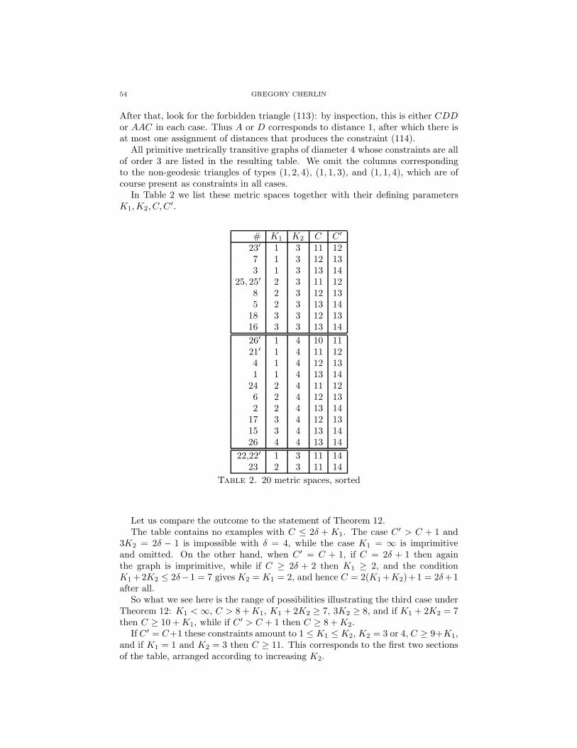
54 GREGORY CHERLIN

After that, look for the forbidden triangle (113): by inspection, this is either CDDor AAC in each case. Thus A or D corresponds to distance 1, after which there isat most one assignment of distances that produces the constraint (114).

All primitive metrically transitive graphs of diameter 4 whose constraints are allof order 3 are listed in the resulting table. We omit the columns correspondingto the non-geodesic triangles of types (1, 2, 4), (1, 1, 3), and (1, 1, 4), which are ofcourse present as constraints in all cases.

In Table 2 we list these metric spaces together with their defining parametersK1,K2, C, C

′.

# K1 K2 C C′

23′ 1 3 11 127 1 3 12 133 1 3 13 14

25, 25′ 2 3 11 128 2 3 12 135 2 3 13 1418 3 3 12 1316 3 3 13 14

26′ 1 4 10 1121′ 1 4 11 124 1 4 12 131 1 4 13 1424 2 4 11 126 2 4 12 132 2 4 13 1417 3 4 12 1315 3 4 13 1426 4 4 13 14

22,22′ 1 3 11 1423 2 3 11 14

Table 2. 20 metric spaces, sorted

Let us compare the outcome to the statement of Theorem 12.The table contains no examples with C ≤ 2δ + K1. The case C′ > C + 1 and

3K2 = 2δ − 1 is impossible with δ = 4, while the case K1 = ∞ is imprimitiveand omitted. On the other hand, when C′ = C + 1, if C = 2δ + 1 then againthe graph is imprimitive, while if C ≥ 2δ + 2 then K1 ≥ 2, and the conditionK1+2K2 ≤ 2δ−1 = 7 gives K2 = K1 = 2, and hence C = 2(K1+K2)+1 = 2δ+1after all.

So what we see here is the range of possibilities illustrating the third case underTheorem 12: K1 < ∞, C > 8 +K1, K1 + 2K2 ≥ 7, 3K2 ≥ 8, and if K1 + 2K2 = 7then C ≥ 10 +K1, while if C′ > C + 1 then C ≥ 8 +K2.

If C′ = C+1 these constraints amount to 1 ≤ K1 ≤ K2, K2 = 3 or 4, C ≥ 9+K1,and if K1 = 1 and K2 = 3 then C ≥ 11. This corresponds to the first two sectionsof the table, arranged according to increasing K2.


If C′ > C + 1 then there is the added constraint C ≥ 8 +K2 and this impliesC = 11, C′ = 14, K2 = 3. Since C > 2δ+K1 we find K1 ≤ 2. This corresponds tothe last two lines of the table.

Part 3. Finite Approximations to the Generic Triangle Free Graph

9. The Finite Model Problem

A structure has the finite model property if every first order sentence true in thestructure is true in some finite structure. A slightly stronger property is the finitesubmodel property, where the finite approximation should be taken to lie withinthe original structure. There is little difference between the notions in the cases ofmost immediate concern here. We focus mainly on the finite model property for thegeneric triangle free graph, and as “triangle free” is part of the first order theoryof this structure, the finite model property and the finite submodel property areequivalent here. We do not necessarily expect the finite submodel property to betrue. There is little evidence either way. But however that may be, it is a concreteproblem of a familiar type in graph theory, and we will take some pains to put itin an explicit form.

This is an attractive problem which has attracted the attention of a number ofcombinatorialists and probabilists, but there is not much to show for it and, inparticular, not much in the literature. So my main task here is to assemble and todocument such information as has come my way about the problem (and to respondmore fully to some occasional queries that have come my way as well).

There is some literature on lower bounds for finite approximations to Fraısse lim-its, in cases where probabilistic considerations guarantee their existence, e.g. [Sz2,Bon09]. We would like to encourage such exploration in cases where the existence ofany such approximation remains in question, and so we will include some relativelyanecdotal information to give a clearer picture of where those explorations mightusefully begin.

9.1. Overview. In general, the theory of a homogeneous locally finite structureis axiomatized by two kinds of axioms: negative axioms defining the “forbiddensubstructures,” e.g. triangles in the case that most concerns us, and extensionproperties stating that for each k, any k-generated subset of k elements may beextended to a (k + 1)-generated subset in any way not explicitly ruled out by thenegative constraints. We will drop all further mention of k-generated structureshere, and suppose that the language is purely relational, so that the issue is one ofextending k given elements by one more element.

In the context of triangle free graphs, the natural extension properties are thefollowing three.

En: for any set A of at most k vertices, and any subset B of A consisting ofindependent vertices, there is a vertex v adjacent to all vertices of B, and to noneof A \B.

E′n: any maximal independent set contains at least k vertices; for any set A of

k independent vertices, and any subset B of A, there is a vertex v adjacent to allvertices of B, and to none of A \B.

Adjn: Any set of at most n independent vertices has a common neighbor.

56 GREGORY CHERLIN

Here the properties En, together with the axiom stating that triangles do notoccur, gives the full axiomatization of the generic triangle free graph. Therefore theproblem of the finite model property for the generic triangle free graph is simplythe question, whether for each n some finite triangle free graph has the extensionproperty En.

The equivalence of En and E′n in triangle free graphs is straightforward, and

with the former more easily applied, and the latter more easily checked. Themutual adjacency condition Adjn is manifestly weaker, but only because it allowssome relatively degenerate examples: the complete bipartite graph, and some lessobvious ones—these can all be satisfactorily classified. As a result, we can replacethe property E′

n by a mild strengthening of Adjn, giving us the simplest version tocheck.

Our first order of business will be to sort out the force of these extension prop-erties. Along the way we will find it useful to classify explicitly all the triangle freegraphs which satisfy the condition Adjn and E2 but not En. For this, a descrip-tion of triangle free graphs satisfying Adj3 in terms of combinatorial geometries isuseful. The geometries in question are formed simply by fixing a vertex v in thegraph, taking its neighbors as points, and the non-neighbors as blocks, with theedge relation in the graph providing the incidence relation in the geometry. Thisslight shift in point of view will simplify both the analysis and the construction ofsuch graphs. This corresponds to the usual construction of the Higman-Sims graph,and while none of our geometries will have a geometry with the elegance of thatgraph’s, that point of view will still be useful.

We refer to triangle free graphs satisfying condition En as n-e.c., which standsfor “n-existentially complete” (for the category of triangle free graphs). This ter-minology comes from model theory.

We will see that there are a number of infinite families of geometries all corre-sponding to 3-e.c. graphs, but that the families known to date are neither variednor robust. In the M22 geometry which is associated with the Higman-Sims graph,every block has 6 points; but in the infinite families of 3-e.c. graphs known to us,there is always at least one block of order 2 (and possibly just one). At the otherextreme, in a geometry associated with a 4-e.c. graph, the minimal block size is atleast 19. Barring some breakthrough taking us to finite 4-e.c. triangle free graphsand beyond, it would be interesting to make the acquaintance of more robust 3-e.c. graphs. We will give explicit descriptions of some infinite families, in the hopesthat this may stimulate someone to find better constructions.

Of the five known non-trivial strongly regular graphs, two provide interestingexamples of 3-e.c. graphs. The question as to whether there are more such tobe found, and possibly an infinite family, seems to be tied up with fundamentalproblems in that subject. However following a suggestion of Peter Cameron, wecan eliminate the possibility that a strongly regular triangle free graph could be4-e.c.

The following general principle is immediate.

Remark 9.1. If M is a structure with the finite model property, and M ′ is astructure which can be interpreted in M , then M ′ inherits the finite model property.

In particular if the generic Kn-free graph has the finite model property for onevalue of n, then so does the generic Km-free for m ≤ n, interpreting the latter asthe graph induced on the set of vertices adjacent to (n−m) vertices of the former.


Thus the finite model property for the generic triangle free graph is the weakestinstance of the problem still open in the case of homogeneous graphs.

One would of course like to have general methods for settling the finite modelproperty in homogeneous structures, but since the most concrete individual casesof the problem remain challenging, we will have to leave that aside.

9.2. Probabilistic methods. One knows the finite model property for the Radograph and similarly unconstrained homogeneous structures by a simple probabilis-tic argument. Just as a random (countable) graph will be isomorphic to the Radograph with probability one, a large finite random graph will have the and one ofthe appropriate extension properties with asymptotic probability 1 [Fag76]. Butprobabilistic constructions behave poorly in the presence of constraints. In partic-ular, with a direct use of counting measure on the set of triangle free graphs of agiven size, a random one will be bipartite with high probability [KPR87], so thatthe theory of the random finite triangle free graph does not approximate the theoryof the generic triangle free graph at all well.

Some time ago Vershik raised the question of a Borel measure invariant under thefull infinite symmetric group and concentrating on the generic triangle free graph,a question answered positively in [PV08] (with a classification of the measures inquestion). But this does not seem to help with the finite model property.

9.3. The Extension properties E2, En, and En′ . We begin by making therelationships between the natural extension properties explicit.

Lemma 9.2. For triangle free graphs G the following properties are jointly equiv-alent to E′

2:

(i) G is maximal triangle free;(ii) G is indecomposable;(iii) G contains an independent set of order 3.

Maximality means that the adjunction of any additional edge would create atriangle, which is the same as the mutual adjacency condition: any two independentvertices have a common neighbor.

A graph is decomposable if it carries a nontrivial congruence, that is, an equiv-alence relation such that for any two classes C1, C2 either all pairs in C1 × C2 areedges, or none are.

Proof. Assume (i − iii). The first point follows from (i, ii). For the second, use(i− ii) to show that a counterexample must be a 5-cycle, and invoke (iii). �

Next we check that the properties E′n and En are equivalent.

Lemma 9.3. For G triangle free, and n arbitrary, properties En and E′n are equiv-

alent.

Proof. Let A be a vertex set of order at most n, and B an independent subset of A.We must show that there is a vertex adjacent to all vertices of B and no verticesof A \B. We proceed by induction on n, and on |A \B|.

If there is an edge (a, b) with a ∈ A \ B and b ∈ B, then let A0 = A \ {a}, andapply induction to n to get v adjacent to all vertices of B, and no vertices of A0 \B,and hence to no vertex of A \B.

58 GREGORY CHERLIN

So we may suppose there is no edge connecting A \ B and B, but that there isan edge in A. In particular |A \ B| ≥ 2. We claim then: There is a vertex u /∈ Awhich is adjacent to some vertex a ∈ A and to no vertex of B.

Let A0 ⊆ A be a maximal independent subset of A containing B, and u a vertexnot adjacent to any vertex of A0. Then u is not in A, and if u is adjacent to somevertex of A we have our claim. So suppose u is adjacent to no vertex of A. Takea ∈ A \B, and a vertex v adjacent to u and a, and to no vertex in B. Then v /∈ A,and v meets the conditions of our claim.

Now applying the claim with u adjacent to a ∈ A and to no vertex of B, letB1 = B ∪ {u}. Let A1 = A \ {a} ∪ {u}. By induction on |A \B| we find v adjacentto all vertices of B1 and no vertex of A1 \B1. Then the set of neighbors of v in Ais B, as required. �

9.4. The strength of Adj3. Our main interest will be in showing that with fewexceptions graphs having the properties E2 and Adjn satisfy the full n-e.c. propertyEn. The delicate case arises when n = 2, and we first dispose of the others.

Lemma 9.4. If G is a 3-e.c. triangle free graph with the mutual adjacency propertyAdjn, then G is n-e.c.

Proof. It suffices to verify the condition E′n. We proceed by induction on n.

Fix A an independent set of order at most n. We may assume |A| = n or concludeby induction. Our objective is to show that every subset of A occurs as the set ofneighbors in A of some vertex of G.

Let us write Av for the set of neighbors in A of the vertex v. Then for v′ chosenadjacent to v and to all vertices of A \Av, we find Av′ = A \Av. So this collectionof sets is closed under complementation in A.

Fix X ⊆ A. We will show that X is Av for some vertex v. Taking complementsif necessary, suppose |X | ≤ n/2. Take a ∈ A \X and u a vertex whose neighborsin A \ {a} are the vertices in X . We may suppose that Au = X ∪ {a}.

Let Y be the complement A \ (X ∪ {a}) and let v be a vertex with Av = Y .If |Y | ≥ 1 then taking u′ (inductively) whose set of neighbors in (A \ Y ) ∪ {v} isX ∪ {v}, we finish.

We conclude that |X | = n− 2, so n = 4 and |X | = 2. In particular any singletonoccurs as Av for some v.

Write A = {a1, a2, b1, b2} and let X = {a1, a2}. Let b′1 be a vertex with Ab′1=

{b1}. Let b2 be a vertex whose unique neighbor in {a1, a2, b′1, b2} is b2. Let u be avertex adjacent to a1, a2, b

′1, b

′2. Then Au = X . �

Now we take up the graphs satisfying E2 and Adj3, but not E3, and we beginwith a construction.

9.5. The Linear Order Geometries. Given any triangle free graph G with themutual adjacency property Adj3 we associate a combinatorial geometry to eachvertex v of G by taking as the set of points P the neighbors of v, and as the blocksof the geometry its non-neighbors. A point p lies on a block b if the pair (p, b)is an edge. The geometry obtained may depend on the vertex chosen, but givenone such geometry, the graph G may be entirely reconstructed as follows. As thevertex set for G we take P ∪B ∪ {v0} where v0 is an additional vertex. We take asedges all pairs (v0, p) with p in P , all pairs (p, b) with p on b, and all pairs (b1, b2)with b1, b2 disjoint when viewed as subsets of P ; and we symmetrize. This agrees


with the original graph G: in particular, if b1, b2 are not adjacent in G, then by theproperty Adj3 there is a point p lying on both, and hence they are not adjacent inthe reconstructed version of G.

The following uses extremely weak assumptions, but then we intend to apply itto an extremely weak geometry.

Lemma 9.5. Let (P,B) be a combinatorial geometry on at least 3 points satisfyingthe following conditions.

(1) No three blocks are pairwise disjoint.(2) No pair of distinct blocks correspond to the same subset of P .(3) For every block b and every point p not in b, there is a block containing p

and disjoint from b.(4) For every pair of points there is a block containing one but not the other.(5) No block is incident with every point of P .

Then the associated graph G is triangle free and 2-e.c.

Proof. One checks that G is maximal triangle free, indecomposable, with an inde-pendent set of size at least three.

One point that requires checking is that no block is empty; this is part of theverification that G is maximal triangle free. For this, use the assumptions to gettwo nonempty blocks which are disjoint, and observe that the empty block wouldextend this to a pairwise disjoint triple. �

Let L be a linear order. Let B be a set of proper initial segments of L and properterminal segments of L satisfying the conditions:

(1) For all a < b in L, there is an initial segment in B containing a and not b,and a terminal segment in B containing b and not a.

(2) If I is an initial segment and a ∈ B \ I is a lub for I, then the terminalsegment [a,∞) is in B; and dually.

One way to meet these conditions is to let B consist of the proper segments ofthe form (−∞, a] and [a,∞), and this is the only way to achieve even the first ofthem if L is finite. Let us call such a geometry a linear geometry.

Lemma 9.6. Let (P,B) be a linear geometry on at least 3 points. Then the as-sociated graph satisfies the conditions E2 and Adjn for all n (if P is finite, this isvacuous for n larger than |P |).Proof. The conditions on the geometry have been written to ensure that our crite-rion for the property E2 applies.

Now suppose A is any independent subset of the associated graph. If A containsno points, then A consists of some blocks, and possibly the base point, and as theblocks all meet pairwise, it suffices to take a point common to the minimal initialsegment in A, and the minimal terminal segment in A. That point is then a vertexadjacent to all vertices of A.

If A contains a point p, then it cannot contain both initial segments and terminalsegments, as they would be separated by p. So suppose for example A containsinitial segments, and let I be the greatest among them. Let a ∈ A be the leastpoint. Then a /∈ I. One of our two conditions on B then applies to give a terminalsegment disjoint from I, and containing a.

Of course if A consists exclusively of points, the base point will suffice as acommon neighbor. �

60 GREGORY CHERLIN

If L is finite of size n, then the resulting graph G has order 3n− 1 and can beconstrued as follows. The elements of G are the integers 0, 1, . . . , 3n− 1; the edgerelation is defined by |i−j| ∼= 1 mod 3. The value n = 2, which is not permitted aswe require 3 points, corresponds to the pentagon, and the first legitimate exampleis a graph of order 8. The maximal independent sets have size n and are the pointsof the geometry, with respect to a basepoint which is their common neighbor. Thegeometry obtained is independent of the base point.

Our next point is that the converse holds: a graph with property E2 and prop-erty Adjn which does not have property En must be obtained in this way from alinear geometry, and in particular if it is finite then it isomorphic to the graph justdescribed explicitly. It will suffice to treat the case n = 3, since once E3 is satisfied,Adjn implies En.

9.6. Graphs with E2, Adj3, and not E3.

Definition 9.7. An independent set of vertices I in a graph G will be said to beshattered if every subset of I occurs as {a ∈ I : a, v are adjacent} for some vertexv.

We will be concerned for the present with graphs which are 2-e.c. but not 3-e.c.,and therefore contain independent triples which are not shattered. We want toshow that within the independent set of all neighbors of any fixed vertex of G, ifone triple is shattered, than all are. We arrive at this gradually by consideringvarious special cases.

Lemma 9.8. Let G be a triangle free graph with properties E2 and Adj3, andsuppose that a, b, c is a shattered independent triple. If a′, b, c is another independenttriple with a, a′ adjacent, then a′, b, c is also shattered.

Proof. Since we have property Adj3, and the collection of sets that can be realizedas sets of neighbors in a′, b, c of vertices of G is closed under complementation, itsuffices to consider a single vertex u ∈ {a′, b, c} and to show that u occurs as theunique neighbor of some vertex among a′, b′c.

For u = a′ we take a as the witnessing vertex. For u = b we take u′ adjacent toa, b and not c. For u = c proceed similarly. �

Lemma 9.9. Let G be a triangle free graph with properties E2 and Adj3, andsuppose that the triple (a, b, c) is independent and not shattered. Then there is aunique vertex u in {a, b, c} which does not occur as the unique neighbor among a, b, cof a vertex in G.

Proof. There must be at least one such vertex, say b. Taking u adjacent to b andnot to a, the neighbors of u among a, b, c will be b and c; and then a commonneighbor of u and a will have a as its unique neighbor among a, b, c; similarly c willoccur as the unique neighbor of some vertex among a, b, c. �

Lemma 9.10. Let G be a triangle free graph with properties E2 and Adj3, andsuppose that I = {a, b, c, d} is an independent quadruple with a, b, c shattered, whilesome vertex u has a and d as its only neighbors in I. Then (b, c, d) is shattered.

Proof. By the previous lemma, the triple u, b, c is shattered, and by another appli-cation of the lemma, b, c, d is shattered. �


Lemma 9.11. Let G be a triangle free graph with properties E2 and Adj3, andsuppose that I = {a, b, c, d} is an independent quadruple with a, b, c shattered, whileno vertex u has precisely two neighbors in I. Then the triple b, c, d is shattered.

Proof. Fix vertices a′, b′, c′ having as their unique neighbors in a, b, c the verticesa, b, or c respectively. By our hypothesis, none of the vertices a′, b′, c′ is adjacentto d.

Now at least two of the vertices a′, b′, c′ are nonadjacent; let u1, u2 be two such.Take v adjacent to u1, u2, and d. Then v is adjacent to at most two vertices ofa, b, c, d and hence, by our hypothesis, to at most one; that is, v is adjacent to dand not to a, b, c.

Suppose now that u1 = a′. Then I ′ = {a′, b, c, d} is an independent quadruplewith a′, b, c shattered, and v has only a′ and d as its neighbors in I ′. By the previouslemma, b, c, d is shattered.

So we may suppose that u1 = b′ and u2 = c′. Then b′, c′, and v has as theirunique neighbors in b, c, d the vertices b, c, and d respectively, and so b, c, d isshattered. �

Lemma 9.12. Let G be a triangle free graph with properties E2 and Adj3, andsuppose that I = {a, b, c, d} is an independent quadruple with a, b, c shattered. Sup-pose there are vertices b′, c′ in G having as their neighbors among a, b, c, d the pairsa, b and a, c respectively. Then b, c, d is shattered.

Proof. The triple b′, c′, d is independent. Let d′ be adjacent to b′, c′, d. Then thevertices b′, c′, d′ show that the triple b, c, d is shattered. �

Lemma 9.13. Let G be a triangle free graph with properties E2 and Adj3, andsuppose that I = {a, b, c, d} is an independent quadruple with a, b, c shattered. Sup-pose there are vertices u, u′ in G having as their neighbors the pairs a, b and c, d,and no other pairs from a, b, c, d occur in this fashion. Then b, c, d is shattered.

Proof. We show first

(5) a, b, d is shattered

This follows by applying Lemma 9.10 to the triples a, b, c, a, b, u′, and a, b, d.Now if a, c, d is shattered, we argue similarly that b, c, d is shattered by looking

at the sequence of triples a, c, d, u, c, d, b, c, d.Take a vertex a′ adjacent to a and not adjacent to b, c. By our hypothesis, a′

is not adjacent to d either. Now take a vertex v adjacent to a′, b, d. Then v is notadjacent to a, so by our hypothesis v is adjacent to c.

We now consider two cases. First, if there is a vertex d′ adjacent to d but not toa, b, c, then we apply Lemma 9.10 to the series of independent triples a, b, d, a, b, d′,a, v, d′, a, c, d′, a, c, d to conclude.

Now suppose that there is no such vertex d′. Then there is no vertex whoseunique neighbor in b, c, d is d. By Lemma 9.9, there is a vertex c′ whose uniqueneighbor among b, c, d is c. Hence, by our hypothesis, c is the only neighbor of c′

among a, b, c, d. If (a, c′) is an edge, we conclude by applying Lemma 9.10 to thesequence of independent triples

(a, b, d); (a′, b, d); (c′, b, d); (c, b, d)

62 GREGORY CHERLIN

So we may suppose (a′, c′) is not an edge. Take a vertex w adjacent to a′, b, c′.Then w is adjacent to b but not a or c, and hence not d either. Now apply Lemma9.10 to the independent triples (a, b, d), (a, w, d), (a, c′, b), (a, c, d) to conclude. �

Lemma 9.14. Let G be a triangle free graph with properties E2 and Adj3, and let Ibe an independent set containing some shattered triple. Then all triples of verticesfrom I are shattered.

Proof. By the foregoing lemmas, if (a, b, c, d) is any independent quadruple con-taining a shattered triple, then all of its triples are shattered. The general casefollows. �

Proposition 9.15. Let G be a triangle free graph with properties E2 and Adj3, butnot E3. Let v be a vertex of G. Then the geometry (P,B) associated to the vertexv in G is a linear geometry, and G is the associated graph.

Proof. G is certainly the associated graph, so everything comes down to recognizingthe geometry on (P,B), with P the set of neighbors of v and B the set of non-neighbors.

We first choose v to be a vertex of G having a triple of neighbors which is notshattered, and let (L,B) be the associated geometry. Once we verify that this isa linear geometry, the structure of G is determined, and it follows that the sameapplies to the geometry at any vertex of G.

We next look for a linear betweenness relation on L. This is a ternary relationβ(x, y, z), irreflexive in the sense that it requires x, y, z to be distinct, which picksout for each triple x, y, z a unique element which is between the other two, i.e.,β(x, y, z) implies β(z, y, x) and not β(y, z, x) or β(z, x, y). In addition to thesebasic properties we have the axiom:

For x, y, z, t distinct, β(x, y, z) implies β(x, y, t) or β(t, y, z)

Any linear order gives rise to a linear betweenness relation, and the reverse ordergives the same betweenness relation; conversely, a betweenness relation determinesa unique pair of linear orders which give rise to it (assuming there are at least twopoints).

We define β(x, y, z) on L as follows: β(x, y, z) holds if any vertex adjacent to y isadjacent to x or z; equivalently (taking complements) any vertex adjacent to x andz is adjacent to y. This is symmetric in x and z, and by Lemma 9.9, the relationpicks out of each independent triple (x, y, z) which is not shattered, a unique ysatisfying β(x, y, z) and β(z, y, x). Furthermore by our choice of v and Lemma9.14, none the triples in L are shattered. So we only have to check the criticalaxiom: assuming β(x, y, z), with t a fourth vertex in L, we claim that β(x, y, t) orβ(t, y, z) holds.

Suppose β(x, y, z) holds and β(x, y, t) fails. We will show that β(t, y, z) holds.As β(x, y, t) fails, we have β(x, t, y) or β(t, x, y).

Suppose β(x, t, y) holds. Take a vertex u adjacent to y and not t. Then byβ(x, t, y), u is not adjacent to x. By β(x, y, z), u is adjacent to z. This provesβ(t, y, z), as claimed.

Now suppose β(t, x, y) holds, and take a vertex u adjacent to y, but not adjacentto z. Then by β(x, y, z) we have u adjacent to x, and by β(x, t, y) we have uadjacent to t. Thus β(t, y, z) holds.


Accordingly, β is a linear betweenness relation on L and we may fix a linearordering giving rise to this relation. By the definition of β, the blocks of B areconvex, and are not bounded both above and below. Therefore they are initialand terminal segments of L (reversing the order will of course interchange thesetwo notions). It remains to check that the blocks are proper, pairwise distinct,and sufficiently dense in L to satisfy our axioms for a linear geometry. This allfollows from the assumption that G satisfies E2, now that the general shape of thegeometry has been established. �

With this result in hand we can give a reasonably efficient axiomatization of thegeometries associated with 3-e.c. graphs.

9.7. Geometries associated with 3-e.c. graphs.

Definition 9.16. An E3-geometry is a combinatorial geometry (P,B) satisfyingthe following axioms.

I There are no three disjoint blocks.II No block is contained in any other.III There are at least two points. For any two distinct points, there is a block

containing exactly one of them, and a block containing neither.IVa If b is a block and p.q are points not in b, then there is a block disjoint from

b containing p and q.IVb If b, b′ are blocks which intersect, and p is a point outside their union, then

some block containing p is disjoint from b and b′.V If three blocks intersect pairwise, then they either have a point in common,

or some block is disjoint from their union.

The E3-geometries are just the geometries associated with 3-e.c. triangle freegraphs, as we shall show. We avoid the seemingly natural term “3-e.c. geometry”,as the natural interpretation for that term would be a considerably stronger setof conditions in which, notably, in axiom V we would require both a point incommon and a disjoint block, that is, we would apply the 3-e.c. condition directlyto the geometry, specifying the type of the element of P ∪ B realizing the givingcondition. The thrust of this is considerably more like 4-e.c. in the correspondinggraph; in fact, it is 4-e.c. restricted to quadruples including the base point. Nodoubt this is an interesting class of geometries in its own right, and more tractablethan those associated with 4-e.c. graphs, but still a good deal beyond anything wecan construct, or analyze, at present.

Lemma 9.17. The geometry associated to any vertex of a 3-e.c. triangle free graphis an E3-geometry, and conversely the graph constructed in the usual way from anE3-geometry is a 3-e.c. triangle free graph.

Proof. One can read off all these axioms directly from the 3-e.c. property (withthe triangle free condition accounting for the first of them). The point is to checkthat conditions (I − −V ) are strong enough. For that, we use the analysis of theprevious subsection. By Axiom II, we exclude the linear geometries of the previoussection, and therefore it suffices to check that the associated graph is triangle free,2-e.c., and satisfies the adjacency condition Adj3, which is more or less what theaxioms assert. �

64 GREGORY CHERLIN

There is still a little redundancy in the set of axioms. It is not actually necessaryto assume explicitly that any two points belong to a block, as long as we assumethere are at least three points, since other axioms contain very similar (and in someways stronger) conditions. Let us use the term “weak E3-geometry” momentarilyfor a geometry satisfying the modified axiom system where we drop the requirementon the existence of blocks containing two specified points, but we add the explicitrequirement that there be at least three points.

Lemma 9.18. Let (P,B) be a weak E3-geometry. Then the union of two blocks isnever P .

Proof. Suppose first that b1, b2 are two blocks which meet, and let p ∈ b2\b1. Thereis a block b′ containing p and disjoint from p1, and as b′ cannot be contained in b,it follows that b1 ∪ b2 6= P .

Now suppose that b1, b2 are disjoint and their union is P . We may suppose that|b1| ≥ 2. Take two points of b1 and a block b containing just one of them. As b isnot contained in b1 and b1 ∪ b2 is P , b meets b2. By construction b ∪ b2 is not P ,so there is a block b′′ disjoint from b ∪ b2. Then b′′ is a proper subset of b1 and wehave a contradiction. �

Lemma 9.19. A weak E3-geometry is an E3-geometry.

Proof. Call two points of P collinear if they lie in a common block. We claim thisis an equivalence relation on P .

Suppose that p, q ∈ b1, and q, r ∈ b2. Take a point a /∈ b1 ∪ b2, and a block bdisjoint from b1 ∪ b2 containing a. As p, r lie outside b, Axiom IVa applies, and p, rare collinear.

By Axiom I, there are at most two equivalence classes for the collinearity relation,and we claim there is only one.

Suppose there are two collinearity classes P1, P2. We may suppose |P1| ≥ 2.Take a block b meeting (and hence contained in) P1. As there are no inclusionsbetween blocks, it follows from Axiom III that b is a proper subset of P1. Thereforeby Axiom IVa we have a block meeting P1 and P2, a contradiction. �

At this point we are through sorting through the basic axioms and we can beginto look more closely at examples of 3-e.c. triangle free graphs and their associatedgeometries. We begin with a quick look at the Higman-Sims graph and stronglyregular triangle free graphs in general.

9.8. The Higman-Sims Graph. This is constructed from the M22 geometry,defined as follows. Let P0 be the projective plane over the field of order 4, with 21points. Adjoin an additional point ∞ to get P = P ∪ {∞}. The associated blockswill be of two kinds. The first kind are obtained by extending an arbitrary line ℓof P0 by the point ∞: ℓ∗ = ℓ ∪ {∞}. The second kind are called hyperovals. Ahyperoval is a set of 6 points in P0 which meets any line of P0 in an even numberof points. There are 168 hyperovals, and on this set the relation “|O1 ∩ O2| iseven” is an equivalence relation, with three classes of 56 hyperovals each, permutedamong themselves by the automorphism group of the base field. Any one class of 56hyperovals may be taken, together with the extended lines, as the set of blocks B forthe M22 geometry, on 22 points. Thus there are 77 blocks, each with 6 points, and100 vertices in the associated graph, the Higman-Sims graph. Its automorphism


group is vertex transitive and edge transitive, so we get the same geometry fromany base point, and any adjacent point can play the role of the “new” point ∞.

We check that this graph is a 3-e.c. triangle free graph. Given three independentvertices, one may be taken to be the base point v, and the other two will thenrepresent two intersecting blocks of the geometry. We may suppose that they bothcontain the point ∞ in the associated geometry, and therefore they represent twoextended lines, whose intersection has order 2. So we have the condition Adj3 withmultiplicity two, that is there are two points meeting the adjacency conditions inevery case. Since the graph visibly satisfies the E2 condition, and there are nocontainments between blocks, this completes the verification that it is 3-e.c. Onthe other hand, it is not 4-e.c. As we know, this comes down to the 4-adjacencyproperty Adj4. Taking a triple of points lying on a projective line ℓ in P0, andanother line meeting ℓ in a different point, a common neighbor of the four verticesinvolved would be a block containing the given three points and disjoint from thegiven line; but there is only one block containing three given points, so this isimpossible.

The Higman-Sims graph is an example of a strongly regular triangle free graph.In general, a graph on n vertices is strongly regular with parameters (n, k, λ, µ) if itis regular of degree k, and any pair of vertices v, v′ has λ common neighbors if v, v′

are adjacent, and µ common vertices otherwise. In the case of triangle free graphs(λ = 0), leaving aside the complete bipartite graphs and the pentagon, there arefive known examples, which go by the names of the Petersen, Clebsch, Hoffman-Singleton, Gewirtz, M22, and Higman-Sims graphs. Two of these graphs are 3-e.c.,the Clebsch graph and the Higman-Sims graph.

While there are no other known strongly regular triangle free graphs, there aremany “feasible” sets of parameters, that is combinations of parameters which arecompatible with all known constraints on such graphs. Following a suggestion ofPeter Cameron, we will use that theory to show that there are no 4-e.c. stronglyregular triangle free graphs, leaving entirely open the problem whether there areany more, or infinitely many more, 3-e.c. strongly regular triangle free graphs.

We will also take a closer look at the known strongly regular triangle free graphs,notably the Clebsch graph, which serves as the basis for the simplest constructionof an infinite family of 3-e.c. graphs, first proposed by Michael Albert.

9.9. Strongly regular graphs and properties E2, E3. Leaving aside the com-plete bipartite graphs and the pentagon, the known strongly regular triangle freegraphs have the following parameters.

(1) Petersen: (10, 3, 0, 1);(2) Clebsch: (16, 5, 0, 2);(3) Hoffman-Singleton: (50, 7, 0, 1);(4) Gewirtz: (56, 10, 0, 2);(5) M22: (77, 16, 0, 4);(6) Higman-Sims: (100, 22, 0, 6)

The “0” here simply says that the graph is triangle free. The Gewirtz graphs andthe M22 graph can be seen naturally inside the Higman-Sims graph (the Hoffman-Singleton graph, less naturally): the Gewirtz graph is the graph on the hyperovalsof the M22 geometry, which could be viewed as the set of vertices in Higman-Simsnonadjacent to two vertices lying on an edge. The M22 graph is the graph on the

66 GREGORY CHERLIN

blocks of the M22 geometry, and appears as the constituent of Higman-Sims on thenon-neighbors of a fixed vertex.

In the Higman-Sims graph, any independent triple of vertices has exactly twocommon neighbors, as noted previously. In particular if the vertices representhyperovals with two common points, then their common neighbors are both repre-sented by points, and hence do not lie in the M22 graph. Thus neither the Gewirtzgraph nor the M22 graph can satisfy the condition Adj3.

The Hoffman-Singleton graph does not fit into this framework at all: there is nouseful geometry induced on the set of neighbors of a fixed vertex. The same appliesto the Petersen graph, but that graph can be viewed as the set of blocks in thegeometry associated to the Clebsch graph, and the latter is indeed a 3-e.c. graph.In the case of the Clebsch graph, the geometry is extremely degenerate: it consistsof all pairs from a set of order 5. Nonetheless this geometry is an E3-geometry.

Thus the Clebsch graph and Higman-Sims graph both are 3-e.c., and the Pe-tersen, Gewirtz, and M22 graphs are naturally represented as descriptions of partor all of the associated geometries.

Any strongly regular graph other than the complete bipartite graphs and thepentagon graph will satisfy the condition E2, and have no proper inclusion betweenblocks, so in all other cases the condition En will be equivalent to the adjacencycondition Adjn.

However the condition Adj4 is already incompatible with strong regularity fortriangle free graphs, as we now show, following the notation of [Big09], which relieson the eigenvalue theory for strongly regular graphs, expressing everything in termsof the minimal eigenvalue for the adjacency matrix of the graph. So we begin byreviewing that material.

9.10. Eigenvalues and E4 in the strongly regular case. Let G be stronglyregular with parameters (n, k, λ, µ). Let A be the n × n adjacency matrix for G,with 0 entries for non-adjacent pairs of vertices, and 1 for adjacent pairs. With Jthe n× n matrix consisting entirely of 1’s, the condition of strong regularity, withthe specified parameters, translates into the matrix condition

A2 + (µ− λ)A − (k − µ)I = µJ

and as J has the eigenvalues n with multiplicity 1 and 0 with multiplicity n − 1,A has three eigenvalues: k with multiplicity 1, and two eigenvalues α, β which areroots of the quadratic equation

x2 + (µ− λ)x − (k − µ) = 0

with multiplicities mα, mβ satisfying

mα +mβ = n− 1;mα · α+mβ · β = 0

since the trace of A is zero. Specializing to the case λ = 0 this gives the followingformulas in terms of the parameter s =

√∆, ∆ being the discriminant µ2+4(k−µ),

an integer in the nontrivial cases (leaving aside the pentagon and complete bipartitegraph):

α =s− µ

2, β =

−s− µ

2


and following [Big09] we write q for the eigenvalue of minimal absolute value (α,above) and express everything in terms of q and µ as follows.

k = (q + 1)µ+ q2

n = (q2 + 3q + 2)µ+ (2q3 + 3q2 − q) + (q4 − q2)µ

− (q + 2)k + (q3 + q2 − q) + (q4 − q2)/µ

µ ≤ q(q + 1)

The inequality on µ is not obvious but is derived rapidly from elementary con-siderations of linear algebra in [Big09].

We note that the extremal values µ = q(q + 1), k = q3 + 3q2 + q, n = q2(q + 3)2

satisfy all known feasibility constraints and give k ≈ (q + 1)3, n ≈ (q + 1 12 )

4, so

that n4 and k3 are fairly close, and as we will see in a moment this makes therefutation of condition E4 a little delicate. Namely, given E4, or what amounts tothe same thing, Adj4, our condition is that the collection of independent 4-tuplesof vertices (u1, u2, u3, u4) should be covered by the independent 4-tuples lying inneighborhoods of the vertices, with the former being slightly less than n4, the latterapproximately n · k4, leading to an estimate of roughly the form k4 > n3. At leastfor large values of n it is clear that this will not be satisfied at the extreme valuesand is less likely to hold lower down. But we will work through this more preciselyto get the following.

Proposition 9.20. There is no strongly regular triangle free graph with the propertyE4.

Proof. Begin with the estimates

n = (q + 2)k + (q3 + q2 − q) + (q4 − q2)/µ

≥ (q + 2)k + (q3 + q2 − q) + (q2 − q)

= (q + 2)k + (q3 + 2q2 − 2q)

≥ (q + 3)k − (µ+ 2q)

≥ (q + 3)k − (q2 + 3q)

Now the number of independent quadruples of vertices in our graph G is at leastn[n− (k+1)][n− 2(k+1)+µ][n− 3(k+1)+µ] and assuming E4, they all occur inneighborhoods of individual vertices, so the number is at most nk(k−1)(k−2)(k−3).So we have

[n− (k + 1)][n− 2(k + 1) + µ][n− 3(k + 1) + µ] ≤ k(k − 1)(k − 2)(k − 3)

and we show this is impossible.We have

[n− (k + 1)] ≥ (q + 2)k − (q2 + 3q + 1)

≥ (q + 2)(k − (q + 1))

and

(n− 2(k + 1) + µ)(n− 3(k + 1) + µ) ≥ [(q + 1)k − (2q + 2)][qk − (2q + 3)]

≥ q(q + 1)(k − 2)(k − (2 + 3/q))

Furthermore q(q + 1)(q + 2) ≥ k + q, so

[n−(k+1)][n−2(k+1)+µ][n−3(k+1)+µ] ≥ (k+q)(k−(q+1)](k−2)[k−(2+3/q)]

68 GREGORY CHERLIN

Suppose µ ≥ q + 1. Then k ≥ (q + 1)2 + q2 ≥ 2q(q + 1), so

(k + q)(k − (q + 1)) = k2 − k − q(q + 1) ≥ k(k − 11

2)

If we take q ≥ 6 as well then we have the estimate

(n− 2(k + 1) + µ)(n− 3(k + 1) + µ) ≥ k(k − 11

2)(k − 2)(k − 2

1

2)

> k(k − 1)(k − 2)(k − 3)

ruling out this case.For q < 6 we may consult the tables in [Big09]. The two cases in which the

necessary inequality holds are one for q = 2, namely the Higman-Sims graph,already ruled out, and one for q = 3, with parameters n = 324, k = 57, µ = 12,where oddly enough the two sides are exactly equal. One way to eliminate this isto show that the block size is too small: later we will give a lower bound of 19 forthe minimal block size in a geometry associated with a 4-e.c. graph.

There remains the marginal case µ ≤ q. In this case as q ≤ 2q2 + q we haven ≥ (q + 3)k + q3 − 3q ≥ (q + 3)k + 3 for q ≥ 3 and thus we can use the crudeestimate

(n− (k + 1))(n− 2(k + 1))(n− 3(k + 1)) ≥ [(q + 2)k][(q + 1)k][qk] ≥ k4

to reach a contradiction. �

Since we have quoted a lower bound for the block sizes in geometries associatedwith 4-e.c. triangle free graphs, we will give that next.

9.11. E4-geometries: Block size. We will refer to a geometry associated witha 4-e.c. triangle free graph as an E4-geometry. We will not try to write out theaxioms explicitly. These would consist of conditions encoding the 2-e.c. propertyas was done in the case of E3-geometries, the condition that no block is containedin another, to eliminate the degenerate case of a linear geometry, and finally themain axioms which correspond to the adjacency condition Adj4 which takes onvarious forms in the geometrical context depending on how the various vertices areinterpreted in the geometry. We may use any instance of the 4-e.c. condition, andare not confined to the special cases corresponding directly to our reduced set ofaxioms.

We omit the elementary proofs of the next few lemmas.

Lemma 9.21. Let (P,B) be an E4-geometry, let b, b1 be intersecting blocks, andlet b2 be any other block. Then

|(b ∩ b1) \ b2| ≥ 2

Lemma 9.22. Let (P,B) be an E4-geometry, let b, b1 be intersecting blocks, Then|b ∩ b1| ≥ 5.

Lemma 9.23. Let (P,B) be an E4-geometry, and let b, b1, b2 be blocks with a pointin common, and b3 a block meeting b but disjoint from b2, b3. Then |b\(b1∪b2∪b3)| ≥5.

Proposition 9.24. Let (P,B) be an E4-geometry. Then any block contains at least19 points.


Proof. Let b be a block. We claim first that there are b1, b2 with b ∩ b1 ∩ b2 6= ∅,and with |(b ∩ b2) \ b1| ≥ 4.

Begin with b∩ b1 ∩ b2 nonempty and with the three blocks distinct, and suppose|(b ∩ b2) \ b1| ≤ 3. Take a block b3 so that:

|b3 ∩ [(b ∩ b2) \ b1]| = 1; b3 ∩ b1 = ∅Then |b ∩ b2 ∩ b3| = 1 and (b ∩ b3) \ b2| ≥ 4.

So fix blocks b1, b2 with b ∩ b1 ∩ b2 6= ∅, and with |(b ∩ b2) \ b1| ≥ 4. Then|b ∩ (b1 ∪ b2)| ≥ 9. Now take b3 disjoint from b1, b2 and meeting b. Then |b ∩ (b1 ∪b2 ∪ b3)| ≥ 14. And then by the previous lemma |b| ≥ 19. �

It would be good to have a more sophisticated lower bound here. We can convertthis bound into a crude but decent lower bound for the number of points in such ageometry.

Lemma 9.25. Let (P,B) be an E4-geometry. Then there are intersecting blocksb1, b2 with |b1 ∪ b2| ≥ 33.

Proof. Let m = min(|b1 ∩ b2 : b1 ∩ b2 6= ∅). If m = 5 we are done.Suppose m ≥ 6. Take any two intersecting blocks b1, b2. Take a block b meeting

b1 and disjoint from b2. Take a point p in b1 \ (b2 ∪ b), and a block b′ disjoint fromb2 containing p.

Then b1, b, b′ meet pairwise and hence by the 4-e.c. condition have a point in

common. Furthermore b1 meets b2 and b, b′ are disjoint from b2. So by Lemma9.23, |b1 \ (b∪ b′ ∪ b2)| ≥ 5. Furthermore |(b1 ∩ b′) \ b| ≥ 2. So |b1 \ (b∪ b2)| ≥ 7 and|b1 \ b2| ≥ m+ 7 ≥ 13.

Also, in the proof of the previous lemma, the lower bound obtained on the blocksize is actually m+ 4+m+ 5 which with m ≥ 6 would give a block size of at least21 and a lower bound for |b1 ∪ b2| of at least 34 in this case. �

Lemma 9.26. Let (P,B) be an E4-geometry, n = |P |. Then n ≥ 66.

Proof. Take intersecting blocks b1, b2 with |b1 ∪ b2| ≥ 33. Let m = min(|b3 ∩ b4| :b3 ∩ b4 6= ∅, (b3 ∪ b4) ∩ (b1 ∪ b2) = ∅). If m = 5 the result is immediate, so takem = 6 and argue as in the previous lemma.

�

Another way of stating all of this is as follows.

Corollary 9.27. Let G be a 4-e.c. graph. Then every vertex has degree at least66, every pair of independent vertices has at least 19 common neighbors, and everytriple of independent vertices has at least 5 common neighbors.

In the Higman-Sims graph the corresponding numbers are 22, 6, and 2.It might be of interest to explore the known feasible parameter sets for strongly

regular triangle free graphs to see which seem compatible with the E3-condition.At the extreme value µ = q(q + 1), the ratio of k(k− 1)(k− 2) to [n− (k + 1)][n−2(k + 1) + µ] is q, which in the two known cases of the Clebsch and Higman-Simsgraphs actually corresponds to the condition Adj3 with multiplicity q. There aremany other cases where the necessary inequality is satisfied with smaller values ofµ. In fact, the majority of the cases listed in the appendix to [Big09] meet thiscondition. The only case consistent with this inequality in which the Adj3 conditionis known to fail is the case of the M22 graph.

70 GREGORY CHERLIN

In a similar vein, dropping the E4 condition. we add some comments on the rela-tionship between the multiplicity with which Adj3 is satisfied, and the multiplicitywith which Adj2 is satisfied.

Let G be a 3-e.c. triangle free graph. Define µn(G) as the minimum over allindependent sets I ⊆ G of order n of the cardinality of the set of common neighborsof I. Thus for example in the Higman-Sims graph, µ2(G) = 6 and µ3(G) = 2.

Lemma 9.28. Let G be a 3-e.c. triangle free graph. If µ3(G) ≥ 2 then µ2(G) ≥ 5.

Proof. Fix two vertices u1, u2 ∈ G, and v adjacent to both. With v as base pointwork in the associated geometry. We look for 4 blocks containing the points u1, u2.

Let b1 be a block containing u1, u2, and u3 ∈ P \b1. Let b2 be a block containingu1, u2, u3 (µ3(G) = 2), and u4 ∈ P \ b1 ∪ b2. Let b3 be a block containing u1, u2, u4.It suffices to show that b1 ∪ b2 ∪ b3 6= P .

Let b be a block containing u4 and disjoint from b1, b2. Then b \ b3 ⊆ P \ (b1 ∪b2 ∪ b3). �

So we have what appears to be a sharply descending series of successive weak-enings of the E4 condition, with no known examples of even the weakest conditionother than subgraphs of the Higman-Sims graph.

(1) G is 4-e.c.(2) µ3(G) ≥ 5(3) µ3(G) ≥ 2(4) µ2(G) ≥ 5(5) µ2(G) ≥ 3(6) In the geometry associated to some base point, every block contains at least

3 points.

What we can do, as mentioned, is produce an infinite family of E3-geometrieswith a unique block of order 2, but even in this case we get no bound on the numberof blocks of order 2 for other geometries associated with the same graph, at differentbasepoints.

We return now to the case of E3-geometries. The first examples of an infinitefamily of 3-e.c. triangle free graphs was given by Michael Albert. An examinationof the corresponding geometries leads naturally to the consideration of a moregeneral class of geometries with rather special properties. From one point of viewthese examples are degenerate; on the other hand, examples can be constructednaturally from projective geometries.

10. Some E3-geometries

10.1. Albert geometries. We first present Michael Albert’s original construction.Observe that the Clebsch graph can be represented as a collection of 4 copiesof a 4-cycle, related systematically to one another: a vertex in one copy will beconnected only to one vertex in any other copy, namely the vertex correspondingto the diagonally opposed to it. Evidently the same recipe can be extended to anynumber of copies of a 4-cycle, and any triple of vertices in one of these extendedgraphs embeds into a copy of the Clebsch graph; so the “stretched” Clebsch graphinherits the 3-e.c. property from the Clebsch graph.

In terms of the associated combinatorial geometry, the Clebsch graph corre-sponds to the geometry on 5 points in which every pair is a block. The stretched


Clebsch graphs correspond to a geometry on n points, n ≥ 5, in which the blocksare of two sorts: (i) all the pairs containing either of two fixed points; (ii) all thesets of points of order n− 3 not containing either of those two points.

Definition 10.1.

1. A point p in a combinatorial geometry (P,B) will be said to be isolated ifevery pair of points containing p is a block.

2. An E3-geometry will be called an Albert geometry if it has at least one isolatedpoint.

Lemma 10.2. For n ≥ 5, there is a unique Albert geometry on n points havingtwo isolated points.

Proof. If p, q are two isolated points, and b is a block not containing p or q, then|b| ≥ n− 3 as otherwise there will be three pairwise disjoint blocks.

Let a ∈ P , a 6= p, q. There is a block b disjoint from the blocks {a, p} and{a, q}, and as |b|gen− 3, b = P \ {a, p, q}. So the identification of the geometry iscomplete. �

We will look at some examples of Albert geometries with a unique isolated point.We do not expect that one can classify these without some further restrictions.In general, the geometry in the associated graph will depend on the base pointselected, so it is noteworthy that if one of these geometries is an Albert geometry,then they all are. We note that even the number of points in the geometry maydepend on the base point, in other words the corresponding graphs are not regularin general. For the specific case of the geometry with two isolated points justdescribed, the corresponding graph is vertex transitive (as is clear from Albert’soriginal description of it), so the same geometry is obtained from any base point.

If we remove an isolated point from an Albert geometry and look at the geometryintroduced on the remaining points, we get a reasonable class of geometries. Thispoint of view is useful for the construction of examples.

Definition 10.3. Let (P,B) be an Albert geometry, a an isolated point. The de-rived geometry (P0, B0) with respect to p has point set P0 = P \ {a}, and blocksB0 = {b ∈ B : a /∈ b}.

The reconstruction of (P,B) from (P0, B0) is immediate. We can phrase theE3-conditions directly in terms of the derived geometry as follows.

I-D There are at least two points.II-D For any three points p, q, r there is a block containing p, q, and not r.III-D There is no inclusion between distinct blocks.IV-D For any block, its complement is a block.V-D If b1, b2, b3 are blocks intersecting pairwise, but with no common point, then

b1 ∪ b2 ∪ b3 6= P0.

Lemma 10.4. If (P,B) is an Albert geometry with a an isolated point then thederived geometry with respect to a satisfies Axioms I-D through V-D. Conversely,if (P0, B0) is a derived geometry, then the combinatorial geometry on P = P0 ∪{a}whose blocks are the blocks of B0 together with the pairs containing a is an Albertgeometry.

We omit the verification. Using this result, we can give examples in a veryconvenient form.

72 GREGORY CHERLIN

Examples 1.

(1) Let (P0, H) be a projective geometry with H the set of hyperplanes. Let(P0, B0) have as its blocks the blocks of H and their complements. This isa derived geometry.

(2) Let (P0, L) be a projective plane and let L′ be a set of lines satisfying oneof the following conditions:(a) Every point lies on at least 3 lines of L′;(b) L′ contains all the line lines of L not passing through some fixed point

p, and two of the lines passing through p.Let L∗ consist of the lines in L′ and their complements. Then (P0, L

∗) isa derived geometry.

(3) Let (P0, L) be a projective plane and ℓ ∈ L a fixed line. Let Lℓ consist ofthe line ℓ together with the sets ℓ∪ℓ1 \ ℓ∩ℓ1 as ℓ1 varies over the remaininglines. Taking these sets and their complements as blocks, we get an Albertgeometry, to which we return below.

(4) Let (P0, H) be as in (1) and let ∞ be an additional point. Extend (P0, H)to (P1, H1) with P1 = P0 ∪ {∞}, H1 = {h ∪ {∞} : h ∈ H}, and let H∗

1

consist of the blocks in H1 and their complements. (P1, H∗1 ) Then (P1, H

∗)is a derived geometry.

(5) Let (P0, B0) be a derived geometry, and a ∈ P0. Let Pa = {b ∈ B0 :a ∈ b} ∪ {∞} with ∞ a new point. Let Ba = P0 \ {a}. For p ∈ Ba letbp = {b ∈ B0 : a ∈ b} ∪ {∞}. Let B∗

a consist of Ba and its complements inPa. Then (Pa, B

∗a) is a derived geometry, as we shall see below. If |P0| = n

and |B0| = 2n′, we will say that the derived geometry has parameters (n, n′).Then (Pa, Ba) has parameters (n′+1, n− 1). If we repeat this constructionto form the geometry Pa∞, Ba∞), we recover (P0, B0).

For example: the derived geometry associated with a projective geometryhas type (n, n) and the new geometry (Pa, Ba) thus has parameters (n +1, n− 1).

As we are ultimately interested in graphs, we need to consider the effect of achange of basepoint.

Proposition 10.5. Let (P,B) be an Albert geometry, G the associated graph, andu ∈ G any vertex. Then the geometry (Pu, Bu) associated to the graph with respectto the base point u is again an Albert geometry.

Proof. Since G is connected, it suffices to prove the claim when u is a point of theoriginal Albert geometry, in other words u is adjacent to the base point v of G.

The case in which u is an isolated point of (P,B) must be handled separately.In this case, there is an involution i ∈ Aut(G) defined by

v ↔ u; a ↔ {a, u}(a ∈ P \ {u}); b ↔ P \ b on blocks

Thus in this case the geometry associated with u is isomorphic to the originalgeometry (P,B).

Suppose now that p0 ∈ P is an isolated point, and u 6= p0. Let p1 = {p0, u} ∈ Pu.We claim that p1 is an isolated point of Pu.

The vertex p0 ∈ Bu is incident with {v, p1} in Pu. For any other b ∈ Pu \{v, p1},we have b ∈ B0, u ∈ b, and b′ = P0 \ b is in Bu, with b′ incident with p1 and b.Thus p1 is an isolated point. �


Tracing through the construction of the associated geometry at the level of thederived geometries, we arrive at our fourth example above. Hence that constructiontakes derived geometries to derived geometries.

Lemma 10.6. Let (P,B) be an Albert geometry, p0 ∈ P an isolated point, and(P0, B0) the corresponding derived geometry with parameters (n, n′) where n = |P0|and n′ = |B0|/2. Let G be the graph associated with (P,B), with base point v. Thenfor any vertex u ∈ B0 ∪ {p0, v}, the associated geometry with base point u has thesame parameters (n, n′), while for u ∈ P0 ∪ (B \ B0), the associated geometry hasparameters (n′+1, n− 1). Thus at most two vertex degrees in the associated graph.

Proof. Let g be the order of the graph G. We have g = 1 + (n+ 1) + (2n′ + n) =2n + 2n′ + 1. For p ∈ P0, the geometry (P,Bp) has parameters (np, n

′p) where

np = |Pp| − 1 with Pp the set of neighbors of p in G, namely v, {p, p0}, and theblocks in B0 which contain p: so np = n′ + 1, and therefore n′

p = n− 1.Making use of the involution v ↔ p0 which interchanges B \B0 and P0, the same

parameters are associated with u ∈ B \B0.On the other hand, for a block b ∈ B0, the set Pb of neighbors of b consists of the

points p belonging to b, the pairs {p0, p} with p ∈ P0 not belonging to b, and thecomplement b′ of b in P0, leading to nb = |Pb| − 1 = |P0| = n and thus n′

b = n′. �

This raises the question as to what sorts of geometries are associated on theone hand with regular graphs, and on the other hand with graphs having just twovertex degrees. These conditions do not seem to be very restrictive, and it maybe of interest to impose similar conditions generalizing strong regularity, perhapsallowing some further use of algebraic methods. As an example, if we begin with theAlbert geometry based on a projective geometry with a single hyperplane removed,we get a regular graph.

Example 1. Let G be the graph associated to the Albert geometry whose derivedgeometry comes from the projective plane. Let v be the base point, p0 ∈ P theisolated point, and ℓ ∈ B a line. The associated geometry has points Pℓ consistingof:

{

points p ∈ P0 lying on ℓ

co-points {p, p0} with p /∈ ℓ

The for ℓ1 6= ℓ a line, the points of Pℓ incident with ℓ as a block in Bℓ are

{p ∈ ℓ \ ℓ1} ∪ {p : p ∈ ℓ1 \ ℓ}In other words, this corresponds to the union of the fixed line ℓ with ℓ1, with theircommon point removed. The block associated with the base point v is {p : p ∈ ℓ}.

In the specific case of the projective plane of order 2, the resulting geometry againcomes from the projective plane of order 2. Otherwise, the geometry is a differentone, and the automorphism group of the graph leaves the pair {v, p0} invariant,and is Aut(P0, B0)× Z2. But for q = 2 the group is transitive on B0 ∪ {p0, v}.10.2. Another series of E3-geometries. Moving away from Albert geometries,what we would like to see next is an infinite family of 3-e.c. graphs G with µ2(G) →∞, ideally even µ3(G) → ∞. But we are far from this. Leaving aside the M22

geometry with its remarkably good properties (µ2(G) = 6, µ3(G) = 2), in infinitefamilies the best we have done to date is to reduce the number of blocks of order

74 GREGORY CHERLIN

2 to a single one, while all other blocks can be made arbitrarily large. But inthis construction we deal with single geometry, rather than the set of geometriesassociated with a given graph. So there is much to be improved on even at thisweak level.

Example 2. With m1,m2,m3 ≥ 2, let the geometry A(m1,m2,m3) be definedas follows. Our pointset consists of three disjoint sets P1, P2, P3 with |Pi| = mi,together with two distinguished points p′, p−, and the following blocks.

(1) b0 = {p, p−} (size 2);(2) For a ∈ Pi: a′ = Pi \ {a} ∪ {p′} (size mi);(3) For a ∈ Pi: a+ = {a} ∪ Pi+1 (addition modulo 3) (size mi+1 + 1);(4) For a ∈ Pi: a− = {a} ∪ Pi−1 ∪ {p−} (size mi−1 + 2).

If m1,m2,m3 ≥ 2 then A(m1,m2,m3) is an E3-geometry, and if m1,m2,m3 ≥3 then it has a unique block of order 2, with the other blocks of order at leastmin(m1,m2,m3). Let G(m1,m2,m3) be the associated graph.

Lemma 10.7. The dihedral group of order 8 acts on G = G(m1,m2,m3) as agroup of automorphisms, extending the natural action on the 4-cycle (v, p′, b0, p

−),with v the base point, b0 = {p′, p−}. In this action the classes P0 = P1 ∪ P2 ∪ P3,B′ = {a′ : a ∈ P0}, B+ = {a+ : a ∈ P0}, and B− = {a− : a ∈ P0} are permuted.

Proof. We define two involutions in Aut(G) by:

ι′ : v ↔ p′ b0 ↔ p− a ↔ a′ a+ ↔ a−

ι− : v ↔ p− b0 ↔ p′ a ↔ a− a+ ↔ a′

�

Lemma 10.8. The graph G(m1,m2,m3) is regular.

Proof. It suffices to check the degree of a vertex a ∈ Pi. The neighbors of a arev, a+, a− and a′1 for a1 ∈ Ai \ {a}, b− for ∈ Ai−1, c

+ for c ∈ Ai−1, for a total of3 + (mi − 1) +mi−1 +mi+1 which is the degree of the base point. �

The geometries associated with G(m1,m2,m3) (i.e., giving an isomorphic graph)are not well behaved.

Lemma 10.9. Let G = G(m1,m2,m3) corresponding to A(m1,m2,m3) with pointset P1 ∪P2 ∪P3 ∪{p′, p−}, and take a ∈ Pi. Then the geometry (Pa, Ba) associatedwith the base point a has at least mi + 1 blocks of order 2, and exactly 2(mi − 1)blocks of order m1 +m2 +m3 − 1 = n− 2 with n = |P | the degree of G. On the setP ∗i = {a′1 : a1 6= a, ai ∈ Pi}∪ {a+, a−} of order mi +1, the induced geometry is the

Albert geometry with two isolated points a+, a−, in the sense that all pairs {a+, a′1}and {a−, a′1} occur as blocks of the associated geometry (Pa, Ba), while all subsetsof order n− 3 contained in Pa which are disjoint from {a+, a−} and which containPa \ P ∗

i also occur as blocks.

Note that in the “restricted” geometry on P ∗i we are taking as blocks, those

which lie within P ∗i , and those which contain its complement.

Proof.

Pa = {v, a+, a−, b′(b ∈ Pi, b 6= a), c−(c ∈ Pi+1), d+(d ∈ Pi−1)}


The block associated with a′ is {a+, a−}. The block associated with b+ for b ∈ Ai,b 6= a is {a−, b′}. The block associated with b− for b ∈ Pi is {a+, b′}.

Finally, the block associated with b ∈ Pi (b 6= a) is

{v} ∪ P−i+1 ∪ A+

i−1 ∪ {b′1 : b1 ∈ Pi, b1 6= a, b}�

We observe that the smallest geometry for which we are able to get a singleblock of order 2 has order 11, namely A(3, 3, 3), and this is sharp. We will givesome additional information concerning small geometries.

10.3. E3-Geometries of order at most 7.

Lemma 10.10. Let (P,B) be an E3-geometry, and n = |P |.(1) The maximal block size is at most n− 3.(2) If there is a block of order n− 3 then all pairs lying in its complement are

blocks.(3) n ≥ 5.(4) If p is a point which is contained in at least n− 3 blocks of order 2 then p

is isolated.(5) If n = 5 or 6 then (P,B) is the Albert geometry with two isolated points.

Proof. The first three points are immediate. For the fourth, let q, q′ be the twopoints not known to occur together with p as a block of order 2. Take a blockcontaining p, q and not q′; it must be {p, q}. Similarly {p, q′} is block.

For the last point, the case n = 5 is immediate, so take n = 6. Then there is apair of points p, q which do not constitute a block, and therefore they are containedin two blocks of order 3, say {p, q, r} and {p, q, s}. Let t /∈ {p, q, r, s}. Then thepairs containing t and neither of p, q are blocks, by our second point. So t is anisolated point. So the geometry has two isolated points, and we are done. �

We will also carry through the analysis for the case n = 7, finding in this casethat the geometry is necessarily an Albert geometry, and that there are only twopossibilities: the Albert geometry with two isolated points, and one other.

Example 3. We construct a derived geometry B′(n1, n2) as follows. Let A1, A2 besets of orders n1, n2 respectively, and c an additional point. Take as blocks:

a1A2(a1 ∈ A1); a2A1(a2 ∈ A2; cA′i(A

′i ⊆ Ai, |Ai \A′

i| = 1)

Let B(n1, n2) be the corresponding Albert geometry, with n1 + n2 + 2 points.

If n1 = n2 = 2 then this is the Albert geometry with two isolated points on 6vertices. Otherwise, it is an Albert geometry with one isolated vertex. In particularwe have the case n1 = 2, n2 = 3 of order 7.

Lemma 10.11. Let (P0, B0) be the derived geometry associated with an Albertgeometry, with n0 = |P0| > 4. Call the blocks of order 2 in B0 edges, and view P0

as a graph with respect to these edges. Then all edges in P0 have a common vertex.

Proof. As n0 > 4 there can be no disjoint edges. So we need only eliminate thepossibility that there is a triangle.

Suppose p, q, r form a triangle: any pair is a block. Take further points s, t,and a block b containing r, s but not t. Then b is disjoint from p, q and hence thecomplement of b is p, q. But then t is in b, a contradiction. �

76 GREGORY CHERLIN

Lemma 10.12. An Albert geometry on 7 points with one isolated point must beisomorphic with B(2, 3).

Proof. We work in the derived geometry (P0, B0) on 6 points, and consider thegraph on P0 whose edges are the pairs occurring as blocks in B0. If there are threeor more edges then their common vertex is a second isolated point, a contradiction.

If there are exactly two edges we identify the geometry B(2, 3) as follows. Letthe vertex v common to the edges be called c, and let the other vertices on theedges be A = {a1, a2}, while the remaining vertices are B = {b1, b2, b3}. As thereare just the two edges, the other blocks containing c are triples of the form {c, b, b′}with b, b′ ∈ B, and as we may exclude any element of B, all such triples occur.Thus we know all the blocks containing c and taking complements, we have all theblocks.

Suppose there is at most one edge, and take four points A = {a1, a2, a3, a4}containing no edge, and let c1, c2 be the other points. Then every block containingc1 and meeting A is a triple, thus the blocks containing c1 meet A in a certain setof pairs E1, and for any two points a, a′ ∈ A there is a pair in E1 containing aand not a′. If E1 contains no disjoint pairs, it follows that the edge set E1 formsa triangle in A; and if we define E2 similarly, and E2 contains no disjoint pairs,then E2 forms a triangle in A. However E1 ∪ E2 covers all pairs in A. So wemay suppose that E1 contains two disjoint pairs, say {a1, a2} and {a3, a4}. Wemay suppose then that E2 contains the pair {a1, a3}, and hence B0 contains theblocks {c1, a1, a2}, {c1, a3, a4}, {c2, a1, a3} which meet pairwise but have no pointin common. But as the union of these blocks is P0, we contradict our axioms. �

And lastly we claim that up to this point no non-Albert geometry occurs.

Lemma 10.13. Let (P,B) be an E3-geometry on n ≤ 7 points. Then (P,B) is anAlbert geometry.

Proof. We have dealt with the cases n < 7 and we suppose n = 7.We call a block of order 2 an edge in P .Suppose first that there is some block A of order 4. We claim that any a ∈ A

lies on an edge.Let A = {a, a1, a2, a3} and take blocks b1, b2 with ai, a3 ∈ bi, a /∈ bi for i = 1, 2.

Take b disjoint from b1 ∪ b2 with a ∈ b. Since any pair disjoint from A is an edge,b must also be an edge.

Now as |A| = 4 we can find two points a1, a2 in A for which there is are edges{p, a1}, {p, a2} with a common neighbor p ∈ P \ A. Then p lies on 4 edges and istherefore an isolated point.

From now on suppose that there is no block of order 4, and we will arrive at acontradiction.

We show first that every point lies on an edge. Suppose the point p lies on noedge, so that every block containing p has order 3. Take two blocks b1, b2 whoseintersection is {p}. Then the complement of b1 ∪ b2 is an edge e.

Take q ∈ b1, r ∈ b2 with q, r 6= p, and with q, r not an edge, using the factthat there are no three disjoint edges. Take a block b3 containing q, r, and not p.Then b1, b2, b3 meet pairwise but have no common point, so they are disjoint froma block, which must be e. Thus b3 ⊆ b1 ∪ b2. There is a point s /∈ b3 ∪ {p} ∪ e.Form a block b containing q, s and not p, and take a block b′ disjoint from b ∪ b3and containing p. Then p ∈ b′ ⊆ {p} ∪ e and thus b′ is an edge containing p.


Now consider the graph on P formed by the edges. Every vertex lies on an edge,there are no three disjoint edges, and furthermore no vertex has degree greater than3, as it would then be an isolated point of the geometry.

By the first two conditions, some vertex p must have degree at least 3, and henceexactly 3. Then it follows by inspection that there is some vertex q not adjacentto p such that every point of P other than p, q is adjacent to one of the two pointsp, q. Consider a block b containing p, q. Since b cannot contain any edge at p or q,b is {p, q}, so these points are adjacent and we have a contradiction. �

10.4. A small non-Albert geometry. We record some further information aboutsmall E3-geometries. The smallest non-Albert geometry lives on a set with 8 points,and is unique up to isomorphism. This geometry has 7 blocks of order 2.

The smallest geometry in which one has a unique block of order 2 is the geometryA(3, 3, 3) on 11 points. If one takes the geometry of lines and hyperovals in theprojective plane over a field of order 4, one gets an example of order 21. On theother hand, we have checked that such a geometry must have 13 points.

By brute force search, all of the E3-geometries of order 8 may be identified.There are such 10 geometries, corresponding to 7 graphs, four of which correspondto two geometries of order 8, two correspond to one geometry of order 8, and the lastcorresponds to one geometry of order 8 and one of order 9. All of these geometriesare Albert geometries except for one pair of geometries corresponding to a singlegraph. We list them as follows, including the block counts (the number of blocksof each size, from the minimum size 2 up to the maximum size). We will refer toone geometry as a “variant” of another if it defines an isomorphic graph.

E3-geometries of order 8:(1) The Albert geometry with two isolated points. Block count (13, 0, 0, 6).(2) Albert geometries with unique isolated points:

(a) The geometry whose derived geometry comes from a projective planeminus a line, with a vertex transitive automorphism group; Block count(7, 6, 6).

(b) The geometry whose derived geometry comes from a projective plane.In the associated graph, there is also a geometry on 9 points. Blockcount (7, 7, 7).

(c) The geometry B(2, 4) with block count (9, 4, 4, 2) and a variant withblock count (7, 6, 6).

(d) The geometry B(3, 3) with block count (7, 6, 6) and a variant withblock count (9, 4, 4, 2).

(e) An Albert geometry with block count (8,5,5,1) and a variant withblock count (7, 6, 6).

(3) A pair of non-Albert geometries with block counts (6, 10, 1, 2) and (7, 6, 6).

11. Appendix: Amalgamation Classes (Data from [Che98])

The following table shows the full list of 27 amalgamation classes determined byconstraints on triangles, not allowing free amalgamation, and with the associatedFraısse limit primitive. The structures are assumed to have three nontrivial 2-types,all of them symmetric (e.g., one may think of these structures as complete graphs,with 3 colors of edges). The data are taken from [Che98].

78 GREGORY CHERLIN

# ABD CDD AAC ADD AAD BBD CCA CCD BDD BAA AAA DDD

1 1 1 0 1 0 0 0 0 0 0 0 02 1 1 0 1 0 0 0 0 0 0 0 13 1 1 0 1 1 0 0 0 0 0 0 04 1 1 0 1 0 0 0 0 0 0 1 05 1 1 0 1 1 0 0 0 0 0 0 16 1 1 0 1 0 0 0 0 0 0 1 17 1 1 0 1 1 0 0 0 0 0 1 08 1 1 0 1 1 0 0 0 0 0 1 19 1 1 0 0 1 0 0 0 0 0 0 1

10 1 0 0 1 0 0 0 0 0 0 1 111 0 1 0 1 0 1 0 0 0 0 0 112 0 1 0 1 1 1 0 0 0 0 0 113 0 1 0 1 0 1 0 0 0 0 1 114 0 1 0 1 1 1 0 0 0 0 1 115 1 1 0 1 0 1 0 0 0 0 0 116 1 1 0 1 1 1 0 0 0 0 0 117 1 1 0 1 0 1 0 0 0 0 1 118 1 1 0 1 1 1 0 0 0 0 1 119 1 1 0 0 1 1 0 0 0 0 0 120 1 1 0 0 1 1 0 0 0 0 1 121 1 1 1 0 1 0 0 0 0 0 0 122 1 1 1 1 1 0 0 0 0 0 0 023 1 1 1 1 1 0 0 0 0 0 0 124 1 1 1 1 0 0 0 0 0 0 1 125 1 1 1 1 1 0 0 0 0 0 1 126 1 1 1 0 1 0 0 1 1 0 0 127 1 0 0 1 1 0 1 1 1 1 1 1

Table 3. 27 amalgamation classes [Che98]. See §8

References

[AH78] F. Abramson and L. Harrington “Models without indiscernibles” J. Symbolic Logic43 (1978), 572–600.

[AL95] R. Akhtar and A. Lachlan, “On countable homogeneous 3-hypergraphs,”Arch. Math. Logic 34 (1995), 331–344.

[AH06] M. Alfuraidan and J. Hall, “Smith’s theorem and a characterization of the 6-cube asdistance-transitive graph,” J. Algebraic Combin. 24 (2006), 195–207.

[AMP10] D. Amato and H. D. Macpherson, Infinite metrically transitive homogeneous graphsof diameter 3, Notes, Spring 2010.

[Ash71] C. Ash, “Undecidable ℵ0-categorical theories,” Notices Amer. Math. Soc. 18 (1971),423.

[Big09] N. Biggs, “Strongly regular graphs with no triangles”, Research Report, September2009. arXiv:0911.2160v1.

[Bon09] A. Bonato, “The search for n-e.c. graphs” Contrib. Discrete Math. 4 (2009), 40–53.[BCN89] A. E. Brouwer, A. M. Cohen, and A. Neumaier Distance-Regular Graphs, Springer-

Verlag, New York, 1989, 485 pp.,[Cam98] “A census of infinite distance transitive graphs” Discrete Math. 192 (1998), 11–26.


[Cam02] P. Cameron Homogeneous permutations, in Permutation patterns (Otago, 2003), Elec-tron. J. Combin. 9 (2002/03), no. 2, Research paper 2, 9 pp.

[Cam96] P. Cameron, “Oligomorphic groups and homogeneous graphs,” NATOAdv. Sci. Inst. Ser. C Math. Phys. Sci., 497, Kluwer Acad. Publ., Dordrecht,1997.

[Cam09] P. Cameron, Oligomorphic permutation groups, London Mathematical Society LectureNote Series, 152. Cambridge University Press, Cambridge, 1990. viii+160 pp.

[Cam80] P. Cameron, “6-transitive graphs,” J. Combinatorial Theory, Series B 28 (1980), ‘68–179.

[Cam96] P. Cameron, “The random graph,” in J. Nesetrril, R. L. Graham (Eds.), The Mathe-matics of Paul Erdos, Springer, Berlin, 1996, pp. 331–351.

[Cam05] P. Cameron “The random graph has the strong small index property,” Discrete Math.291 (2005), 41–43.

[Che93] “Combinatorial Problems connected with finite homogeneity” Proceedings of the In-ternational Conference on Algebra, Part 3 (Novosibirsk, 1989), 3–30, Contemp. Math.131, Part 3, Amer. Math. Soc., Providence, RI, 1992.

[Che88] G. Cherlin, “Homogeneous tournaments revisited,” Geom. Ded. 26 (1988), 231-240.[Che99] G. Cherlin, “Infinite imprimitive homogeneous 3-edge-colored complete graphs,”

J. Symbolic Logic 64 (1999), 159–179.

[Che98] G. Cherlin, “The classification of countable homogeneous directed graphs and count-able homogeneous n-tournaments.” Mem. Amer. Math. Soc. 131 (1998), no. 621,xiv+161 pp.

[CL00] G. Cherlin and B. Latka Minimal antichains in well-founded quasi-orders with anapplication to tournaments, J. Combin. Theory Ser. B, 80 (2000), 258–276.

[CSW] “On homogeneous nilpotent groups and rings” Proc. Amer. Math. Soc. 119 (1993),1289–1306.

[CT] G. Cherlin and S. Thomas, “Two cardinal properties of homogeneous graphs,” J. Sym-bolic Logic 67 (2002)

[DNT86] J. Dixon, P. Neumann, and S. Thomas, “Subgroups of small index in infinite symmetricgroups,” Bull. London Math. Soc. 18 (1986), 580-586.

[Dun82] M. J. Dunwoody, Cutting up graphs. Combinatorica 2 (1982), 15–23.[Ehr72] A. Ehrenfeucht, “There are continuum ℵ0-categorical theories,” Bull. Acad. Polon. Sci.

20 (1972), 425-427.[Fag76] R. Fagin, “Probabilities on finite models,” J. Symb. Logic 41 (1976), 50-58.[Fra54] “Sur l’extension aux relations de quelques proprietes des ordres,” Ann. Ecole Normale

Sup. 7 (1954), 361–388.[Gar76] A. Gardiner, “Homogeneous graphs,” J. Comb. Th. 20 (1976), 94-102.[Gla71] W. Glassmire, Jr. “There are 2ℵ0 countably categorical theories,”

Bull. Acad. Polon. Sci. 19 (1971), 185–190.[GK09] L. Graham, J. M. Kantor, Naming Infinity: A True Story of Religious Mysticism and

Mathematical Creativity, Belknap Press of Harvard University Press, 2009.[Hen71] C. W. Henson, “A family of countable homogeneous graphs,” Pacific J. Math. 38

(1971), 69–83.[Hen72] C. W. Henson, “Countable homogeneous relational systems and categorical theories,”

J. Symb. Logic 37 (1972), 494-500.[HHLS93] W. Hodges, I. Hodkinson, D. Lascar, and S. Shelah, “The small index property for

ω-stable ω-categorical structures and for the random graph,” J. London Math. Soc.48 (1993) 204–218.

[HN05] J. Hubicka and J. Nesetril, “Finite presentation of homogeneous graphs, posets andRamsey classes,” Probability in mathematics, Israel J. Math. 149 (2005), 21–44.

[Hus08] M. Husek, “Urysohn space, its development and Hausdorff’s approach” Topology andits Applications 155 (2008), 1493–1501. Special number devoted to the proceeedingsof a Workshop on the Urysohn space, Beer-Sheva, 2006.

[KPT05] A. Kechris, V. Pestov, and S. Todorcevic, “Fraısse limits, Ramsey theory, and topo-logical dynamics of automorphism groups,” Geom. Funct. Anal. 15 (2005), 106–189.

[GK78] Ya. Gol’fand and Yu. Klin “On k-homogeneous graphs,” (Russian), Algorithmic stud-ies in combinatorics (Russian) 186, 76–85, (errata insert), “Nauka”, Moscow, 1978.

[KG] A. Klin and Golfand

80 GREGORY CHERLIN

[KPR87] Ph. Kolaitis, H. Promel, and B. Rothschild, “Kℓ+1-free graphs: asymptotic structureand a 0-1 law,” Trans. Amer. Math. Soc. 303 (1987), 637-671.

[Kom99] P. Komjth, “Some remarks on universal graphs,” Discrete Math. 199 (1999), 259–265.[KMP88] P. Komjath, A. Mekler and J. Pach. Some universal graphs, Israel J. Math, 64 (1988),

158–168.[KT01] D. Kuske and J. Truss, “Generic automorphisms of the universal partial order,”

Proc. Amer. Math. Soc. 129 (2001), 1939–1948.[Lac86] A. Lachlan “Binary Homogeneous Structures II,” Proc. London Math. Soc. 52 (1986),

412–426.[Lac84] A. Lachlan “Countable homogeneous tournaments,” Trans. Amer. Math. Soc. 284

(1984), 431-461.[Lac86] A. Lachlan “Homogeneous structures,” in Proceedings of the ICM 1986, American

Mathematical Society, 1987, 314-321.[Lac82] Lachlan, A. H.(3-SFR) “Finite homogeneous simple digraphs,” Proceedings of the

Herbrand symposium (Marseilles, 1981), 189–208, Stud. Logic Found. Math., 107,North-Holland, Amsterdam, 1982.

[Lac96] “Stable finitely homogeneous structures: a survey,” Algebraic model theory (Toronto,ON, 1996) 145–159, NATO Adv. Sci. Inst. Ser. C Math. Phys. Sci., 496, Kluwer Acad.Publ., Dordrecht, 1997.

[LT95] A. Tripp and A. Lachlan, “Finite homogeneous 3-graphs,” Math. Logic Quart. 41

(1995), 287–306.[LW80] A. Lachlan and R. Woodrow, “Countable ultrahomogeneous undirected graphs,”

Trans. Amer. Math. Soc. 262 (1980), 51-94.[Lat94] B. J. Latka. “Finitely constrained classes of homogeneous directed graphs,”

J. Symb. Logic, 59:124–139, 1994.[La03] B. J. Latka. “A structure theorem for tournaments omitting N5,” J. Graph Theory

42 (2003), 165–192.[La02] B. J. Latka. “A structure theorem for tournaments omitting IC3(I, I, L3),” Preprint,

1994, revised 2002.[Mph82] H. D. Macpherson, Infinite distance transitive graphs of finite valency. Combinatorica

2 (1982), 63–69.[Nes07] J. Nesetril, “Metric spaces are Ramsey,” European J. Combin. 28 (2007), 457–468.[NR75a] J. Nesetril and V. Rodl, “A Ramsey graph without triangles exists for any graph

without triangles,” Infinite and Finite Sets (Colloq., Keszthely, 1973; dedicated toP. Erdos on his 60th birthday, Vol. III, 1127–1132. Colloq. Math. Soc. Janos Bolyai10, North-Holland, Amsterdam, 1975.

[NR77a] J. Nesetril and V. Rodl, “A structural generalization of the Ramsey Theorem,”Bull. Amer. Math. Soc. 83 (1977), 127–128.

[NR90] J. Nesetril and V. Rodl, eds., Mathematics of Ramsey theory, Algorithms and Com-binatorics, 5. Springer-Verlag, Berlin, 1990. xiv+269

[NR77b] J. Nesetril and V. Rodl, “Partition of relational and set systems,” J. Combin. TheorySer. A 22 (1977), 289–312.

[NR83] J. Nesetril and V. Rodl, “Ramsey classes of set systems,” J. Combin. Theory Ser. A34 (1983), 183–201.

[NR] J. Nesetril and V. Rodl, “The Ramsey property for graphs with forbidden completesubgraphs,” J. Combin. Theory Ser. A 20 (1976), 243–249.

[NR75b] J. Nesetril and V. Rodl, “Type theory of partition properties of graphs,” Recent Ad-vances in Graph Theory (Proc. Second Czechoslovak Sympos., Prague, 1974 405–412,Academia, Prague, 1975.

[Pes02] V. Pestov, “Ramsey-Milman phenomenon, Urysohn metric spaces, and extremelyamenable groups” Israel J. Math. 127 (2002), 317–357.

[PV08] F. Petrov and A. Vershik, “Invariant measures on the set of graphs and homogeneousuncountable universal graphs,” Preprint, 2008.

[Rad64] R. Rado. “Universal graphs and universal functions,” Acta Arith. 9 (1964), 331–340.[Rub94] M. Rubin, “On the reconstruction of ℵ0 categorical structures from their automor-

phism groups,” Proc. London Math. Soc. 69 (1994), 225–249.


[SW85] D. Saracino and C. Wood, “Finite homogeneous rings of odd characteristic,” Logiccolloquium ’84 (Manchester, 1984), 207–224, Stud. Logic Found. Math., 120, North-Holland, Amsterdam, 1986.

[Sch79] J. Schmerl, “Countable homogeneous partially ordered sets,” Alg. Univ. 9 (1979),317-321.

[She74] “Smoothly embeddable subgraphs,” J. London Math. Soc. 9 (1974), 212-218.[Smi71] D. Smith, “Primitive and imprimitive graphs,” Quart. J. Math. Oxford 22, (1971),

551–557.[Sz2] E. Szekeres and G. Szekeres “On a problem of Schutte and Erdoos,” Math. Gazette

49 (1965), 290–293.[Tho91] S. Thomas, “Reducts of the random graph,” J. Symbolic Logic 56 (1991), 176–181.[Tho91] S. Thomas, “Reducts of random hypergraphs,” Ann. Pure Appl. Logic 80 (1996),

165–193.[TT08] “Countable homogeneous coloured partial orders,” Dissertationes Math. (Rozprawy

Mat.) 455 (2008), 48 pp.[Tr09] J. Truss, “Generic automorphisms of homogeneous structures,” Proc. London

Math. Soc. 65 (1992), 121–141.[Tr09] J. Truss, “On the automorphism group of the countable dense circular order,”

Fund. Math. 204 (2009), 97–111.

[Tru03] J. Truss, “The automorphism group of the random graph: four conjugates good, threeconjugates better,” Discrete Math. 268 (2003), 257–271.

[Tru85] J. Truss, “The group of the countable universal graph,” Math. Proc. CambridgePhil. Soc. 98 (1985), 213-245.

[Ury25] “Sur un espace metrique universel,” CRAS 180 (1925), 803–806.[Ury27] “Sur un espace metrique universel,” Bull. Sci. Math. 51 (1927), 43–64 and 74–90.

Department of Mathematics//Rutgers University// 110 Frelinghuysen Rd.//Piscataway,NJ 08854

E-mail address: [email protected]

TWO PROBLEMS ON HOMOGENEOUS STRUCTURES, REVISITEDcherlin/Publication/census.pdf · TWO PROBLEMS ON...

Documents

Transcript of TWO PROBLEMS ON HOMOGENEOUS STRUCTURES, REVISITEDcherlin/Publication/census.pdf · TWO PROBLEMS ON...