Two New Algorithms for UMTS Access Network

Topology Design

Alpar Juttner∗†, Andras Orban∗, Zoltan Fiala∗

September 17, 2003

Abstract

Present work introduces two network design algorithms for planning

UMTS (Universal Mobile Telecommunication System) access networks.

The task is to determine the cost-optimal number and location of the

Radio Network Controller nodes and their connections to the Radio Base

Stations (RBS) in a tree topology according to a number of planning con-

straints. First, a global algorithm to this general problem is proposed,

which combines a metaheuristic technique with the solution of a specific

b-matching problem. It is shown how a relatively complex algorithm can

be performed within each step of a metaheuristic method still in reasonable

time. Then, another method is introduced that is able to plan single RBS-

trees. It can also be applied to make improvements on each tree created

by the first algorithm. This approach applies iterative local improvements

using branch-and-bound with Lagrangian lower bound. Eventually, it is

demonstrated through a number of test cases that these algorithms are

able to reduce the total cost of UMTS access networks, also compared to

previous results.

Keywords: Telecommunication, Metaheuristics, UMTS, Facilities planning

and design, Lagrange–relaxation

∗Ericsson Research Hungary, Laborc u.1, Budapest, Hungary H-1037

e-mails: {Alpar.Juttner,Andras.Orban,Zoltan.Fiala}@eth.ericsson.se†Communication Networks Laboratory and Department of Operations Research, Eotvos

University, Pazmany Peter setany 1/C, Budapest, Hungary H-1117

1

1 Introduction

UMTS [24], [21] stands for Universal Mobile Telecommunication System; it is

a member of the ITU’s IMT-2000 global family of third-generation (3G) mobile

communication systems. UMTS will play a key role in creating the future mass

market for high quality wireless multimedia communications, serving expectedly

2 billion users worldwide by the year 2010.

One part of the UMTS network will be built upon the transport network

of today’s significant 2G mobile systems [14], but to satisfy the needs of the

future Information Society new network architectures are also required. Since

UMTS aims to provide high bandwidth data, video or voice transfer, the radio

stations communicating with the mobile devices of the end-users should be placed

more dense to each other, corresponding to the higher frequency needed for the

communication. In the traditional star topology of the radio stations, i. e. all the

radio stations are directly connected to the central station, this would increase

the number of expensive central stations as well. To solve this problem, UMTS

allows a constrained tree topology of the base stations, permitting to connect

them to each other and not only to the central station. This new architecture

requires new planning methods as well.

As shown in Figure 1 the UMTS topology can be decomposed into two main

parts: the core network and the access network. The high-speed core network

based on e. g. ATM technology connects the central stations of the access network.

These connections are generally realized with high-capacity optical cables. In this

paper the focus is on planning the access network, the design of the core network

is beyond the scope. The reader is referred to e. g. [20] on this topic.

The access network consists of a set of Radio Base Stations (RBS nodes)

and some of them are provided with Radio Network Controllers (RNC nodes).

The RBSs communicate directly with the mobile devices of the users, like mobile

phones, mobile notebooks, etc., collect the traffic of a small region and forward it

to the RNC they belong to using the so-called access links, that are typically mi-

crowave radio links with limited length (longer length connections can be realized

using repeaters, but at higher cost). In traditional GSM configuration the RBSs

are connected directly to an RNC station limiting the maximum number of RBSs

2

CORE NETWORK

RBS

RNC

R

A B

inter−RNC andcore network links

access links

Figure 1: UMTS topology

belonging to a certain RNC. To overcome this limitation the UMTS technology

makes it possible for an RBS to connect to another RBS instead of its RNC.

However RBSs have no routing capability, they simply forward all the received

data toward their corresponding RNC station, therefore all traffic from an RBS

goes first to the RNC controlling it. For example if a mobile phone in region A

on Figure 1 wants to communicate with a device in region B, their traffic will

be sent trough the RNC R. Only the RNC station is responsible for determining

the correct route for that amount of traffic. It follows that the RBSs should

be connected to the RNC in a tree topology. ( There are research initiatives to

provide some low-level routing capability for the RBSs and to allow additional

links between RBSs, which may increase the reliability of the network. These

developments are quite in early stage, hence we only deal with tree topology.)

As a consequence, the access network can be divided into independent trees of

RBSs, each rooted at an RNC. These trees are called Radio Network Subsystems

(RNS). Further advantage of the tree topology compared to the star topology is

that the links can become shorter, which on one hand reduces the cost of the

links, on the other hand it may require less repeaters in the network.

Moreover, there are some additional links connecting the RNCs to each other

(inter-RNC links) and to the core network. The planning of these links are

beyond the scope of this paper.

For technical reasons the following strict topology constraints have to be taken

3

into account:

• The limited resources of the RBS stations and the relatively low bandwidth

of the access links cause considerable amount of delay in the communication.

In order to reduce this kind of delay, the maximum number of the access

links on a routing path is kept under a certain amount by limiting the depth

of a tree to a small predefined value. This limit is denoted by ltree in our

model. Currently, the usual value of ltree is 3.

• The degree of an RBS is also constrained. One simple reason is that the

commercial devices have only limited number of ports. Another reason

is that too many close RBSs can cause interference problems in their ra-

dio interface if their connections are established through microwave links.

Moreover the capacity of an RBS device also limits the number of con-

nectable RBSs. Therefore in our model there can be at most dRBS RBSs

connected directly to another RBSs on a lower level. It is typically a low

value, dRBS = 2 in the currently existing devices.

• The degree of RNCs (the number of RBSs connected directly to a certain

RNCs) is also limited for similar reasons, it is at most dRNC . Generally

dRNC � dRBS.

The planning task investigated in the present paper is to plan cost-optimal

access network, that is to determine the optimal number and location of the RNCs

and to find the connections of minimal cost between RNCs and RBSs satisfying

all the topological restrictions.

The cost of a UMTS access network is composed of two variable factors: the

cost of the RNC stations and the cost of the links. For the exact definitions see

Section 2.

Unfortunately, this planning problem is NP-hard. The problem of finding a

minimal weight two-depth rooted tree in a weighted graph can be reduced to this

problem. Moreover, the problem remains NP-hard even in the special case of

planning a single tree with a fixed RNC node. See Appendix A for the proof of

this claim.

A general UMTS network may contain even about 1000 RBSs, a powerful

RNC device controls approximately at most 200-300 RBSs. This large number

4

of network nodes indicates that the planning algorithms have to be quite fast in

order to get acceptable results.

One possible approach to the problem described above would be to divide the

set of input nodes into clusters and then create a tree with one RNC in each

cluster. However, this “two-stage” solution has some significant drawbacks: first,

it is very hard to give a good approximation to the cost of a cluster without

knowing the exact connections. Second, it would be also a strong restriction to

the algorithm searching for connections to work in static clusters of nodes created

in the beginning.

For these reasons a “one-stage” approach is introduced: an algorithm which

creates a number of independent trees with connections simultaneously. The

proposed method called Global is based on a widely used metaheuristic tech-

nique called Simulated Annealing. However, it is not straightforward to apply

Simulated Annealing to this problem, since the state space is very large and a rea-

sonable neighborhood-relationship is hard to find. To overcome these problems

a combination of the Simulated Annealing and a specific b-matching algorithm

is proposed. To make this method efficient it will be shown how the relatively

complex and time-consuming b-matching method can be performed within each

step of a metaheuristic process in still acceptable time.

Then, a Lagrangian relaxation based lower bound computation method is

presented for the problem of designing a single tree with predefined RNC node.

Using this lower bound a branch-and-bound method is proposed to compute the

theoretical optimal solution to this problem for smaller but still considerable large

number of nodes.

For bigger single-tree design tasks, a second heuristic method called Local is

proposed based on an effective combination of a local search technique and the

branch-and-bound procedure above. This Local algorithm can be used effectively

either in circumstances when only a single tree should be designed or to improve

each trees provided by the Global algorithm.

Related work. Similar problems have already been examined by several au-

thors, using different notations according to the origin of their optimization tasks.

By adding a new virtual root node r to the underlying graph and connecting

5

the possible RNC nodes to r the problem transforms to the planning problem of

a single rooted spanning tree with limited depth and with inhomogeneous degree

constraints. There are some papers in the literature dealing with planning a

minimal cost spanning tree with either of the above constraints (see e. g. [17, 18,

2]), but finding an algorithm handling both requirements is still a challenge.

On the other hand, our problem can be considered as a version of facility

location problems. The problem of facility location is to install some “facilities”

at some of the possible places, so that they will be able to serve a number of

“clients”. The objective is usually to minimize the sum of distances between the

clients and the corresponding facilities while satisfying some side constraints, e.

g. the number or capacity of facilities is limited. See e. g. [9, 19] for more details

on facility location problems and on the known algorithmic approaches.

Facility location problems give a good model to the planning task of tra-

ditional GSM access network topology, for it requires the design of one-level

concentrators. The case of multilevel concentrators is also studied in the liter-

ature, though less extensively. [22] examined the problem similar to ours, but

without depth and degree constraint and with capacity dependent cost functions.

[5] discusses the case of two-level concentrators, also without degree constraints.

Finally, our problem can also be considered as an extension of the so-called hub

location problem. In this scenario we have a given set of nodes communicating

with each other and the amount of the traffic between the node pairs is given by

a traffic matrix. Instead of installing a link between every pair of nodes, each

node is connected to only a single special node called hub. The hubs are fully

interconnected, so the traffic flow between two nodes is realized on a path of

length three, where the two intermediate nodes are hubs. The task is to find an

optimal placement of hubs, where the cost is composed of the cost of the hubs

and the capacity dependent cost of the links. There are several papers examining

hub location problems with various side constraints and optimization objectives.

A good review on this topic can be found e. g. in [16].

A previous method that is able to a give solution to the problem presented in

this paper can be found in [13]. This algorithm called TreePlan finds the number

and the places of the RNC devices by Simulated Annealing metaheuristic and

connects the nodes to the RNSs using an extension of Prim’s spanning tree algo-

6

rithm, which respects the topological requirements on the tree. This algorithm

was used as a reference method in our experimental tests.

The rest of the paper is organized as follows. First, in Section 2 the exactly

defined planning problem is introduced. Then, in Section 3 the Global algorithm

for the general problem is described in detail. In Section 4 the Local method

is introduced for planning a single tree with one RNC. Section 5 shows the re-

sults of test cases of both algorithms also compared to former solutions. Finally,

Appendix A gives a short proof of the NP-completeness of the problem in the

special case when only a single tree with a given RNC node is planned.

2 Problem Definition and Notations

The access network is modeled as a directed graph G(N, E), where N is the set of

the RBSs. For each feasible solution there exists a natural one to one mapping of

the set of links to the set of edges. Each edge in E corresponds to a link between

its ends and directed toward the corresponding RNC. On the other hand, this set

E of directed edges determines the set of RNCs as well: a node is RNC if and

only if it has no outgoing edge.

In order to illustrate the logical structure of the network the notion of the

level of nodes is introduced (Figure 2). Let all RNC nodes be on level 0, and let

the level of an RBS station be the number of edges of the path that connects it

to its controlling RNC. The level of a link is defined as the level of its end on

the greater level-number. Some other important notations used in this paper is

shown in Table 1.

RBS

RNC

0. level

1. level

2. level

3. level

Figure 2: Logical structure of the network

7

N the set of RBSs

E the set of links

n the number of network nodes

ltree the maximal depth of the trees

LEi , Li the set of nodes on the i-th level of the graph

Ei the set of links on the i-th level of the graph

lE(v), l(v) the level of the node v

lE(e), l(e) the level of the edge e

dRBS the maximal degree of an RBS

dRNC the maximal degree of an RNC

costRNC the cost of an RNC

Table 1: Some important notations

The input of the examined planning problem consists of the set N of RBSs,

the cost function clink of the links (described later), the installation cost costRNC

of the RNCs and the constraints dRNC , dRBS and ltree. Moreover we are given

the set RR of places of required RNCs and the set RP of places of possible RNCs.

(It is useful since in many practical cases already existing networks should be

extended.)

The set E of links is a feasible solution to this input if

• E forms a set of disjoint rooted trees, which cover the whole set N ,

• the depth of each tree is at most ltree,

• the degree of the root of each tree is at most dRNC ,

• the in-degree of each other node is at most dRBS,

• RR ⊆ LE0 ⊆ RP .

The total cost of the network is composed of the following factors.

• The cost of the RNC stations. The cost of one RNC, costRNC , means the

installation cost of that particular RNC. This constant may contain other

8

factors as well, e. g. the cost of the links between the RNCs can be included,

assuming that it has a nearly constant additional cost for every RNC.

• The cost of the access links. In this model the cost clink(i, j, l) of a link

depends on its endpoints i and j and its level l. A possible further simpli-

fication is to assume that clink(i, j, l) = fl · clink(i, j), where fl is a constant

factor representing the weight of level l.

This kind of link-cost function has two applications. First, since access

links closer to the RNC aggregate more traffic, this is an elementary way

to model the capacity dependent costs by giving higher cost on the lower

levels. Second, it can be used to prohibit the usage of some links on some

levels by setting their cost to an extremely large value. Also, it makes it

possible to force a node to be on a predefined level.

So, the task is to find a feasible connection E minimizing the total cost

|LE0 | · costRNC +

∑(ij)∈E

clink

(i, j, lE

((ij)))

(1)

3 The Global Algorithm

The aim of this algorithm is to find the optimum places of the RNC nodes (i. e. to

decide which RBSs should be equipped with RNC devices) and to connect each

RBS to an RNC directly or indirectly as described in Section 2. The basic idea

of the proposed approach is the following.

Assuming that the level l(v) is known for each node v, the theoretically min-

imal cost can be determined for that given level-distribution (see Section 3.2).

The algorithm considers a series of such distributions, determines the cost for

each of them and uses some metaheuristic method to reach the final solution.

From among the wide range of metaheuristic methods existing in the literature,

Simulated Annealing was chosen for this purpose, but some other local search

methods could also be used, e. g. the so-called Tabu Search method [11, 1].

9

3.1 Using Simulated Annealing

In this section the application of Simulated Annealing ([15, 1]) to the problem

is illustrated. To use Simulated Annealing to a specific optimization problem,

an appropriate state space S corresponding to the possible feasible solutions,

a neighborhood-relation between the states and a cost function of each state

should be selected. The role of neighborhood-relation is to express the similarity

between the elements of the state space. The neighborhood of a state s is typically

defined as the set of the states that can be obtained by making some kind of local

modifications on s.

Then the Simulated Annealing generates a sequence of feasible solutions

s0, s1, · · · , approaching to a suboptimal solution as follows. It starts with an

arbitrary initial state s0. In each iteration it chooses a random neighbor si+1 of

the last solution si and calculates its cost c(si+1), then decides whether it accepts

this new solution or rejects it (i. e. si+1 := si). This iteration is repeated until a

certain stop condition fulfills.

If the cost of the new state c(si+1) is lower than c(si), the new state is always

accepted. If it is higher then it is accepted with a given probability Paccept de-

termined by the value of the deterioration and a global system variable, the so

called temperature T of the system. In this case Paccept is also positive, however,

it is an exponentially decreasing function of cost deterioration.

In general, the state si+1 is accepted with probability

Paccept = min

{1, exp

(−c(si+1)− c(si)

Ti

)}.

The temperature decreases exponentially during the execution, i.e the tem-

perature Ti in the i-th iteration is given by:

Ti = Ti−1 ∗ fact, T0 = const.

where fact is the so called decreasing factor, which is a number close to 1,

typically 0.99-0.9999. The values T0 and fact are declared in the beginning of

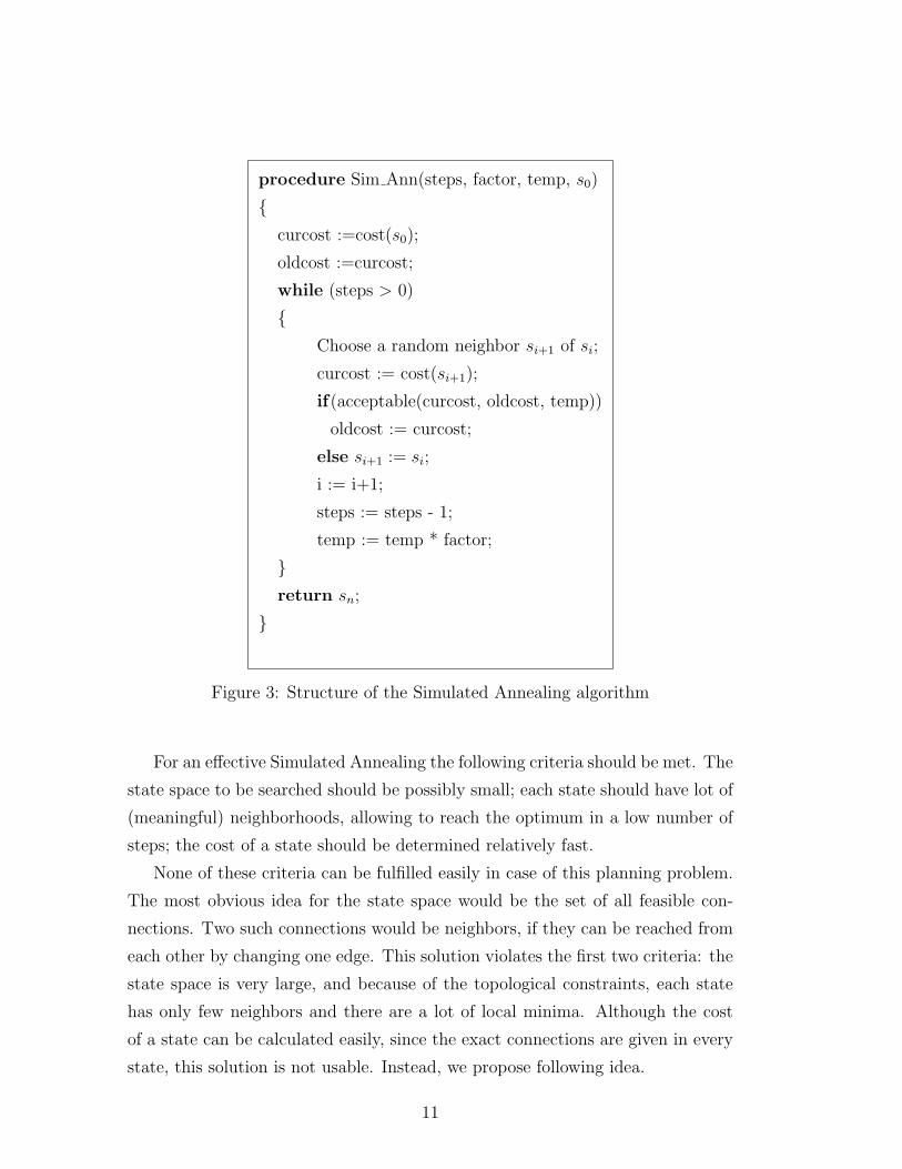
the algorithm. The short pseudo-code in Figure 3 illustrates the framework of

Simulated Annealing.

10

procedure Sim Ann(steps, factor, temp, s0)

{curcost :=cost(s0);

oldcost :=curcost;

while (steps > 0)

{Choose a random neighbor si+1 of si;

curcost := cost(si+1);

if(acceptable(curcost, oldcost, temp))

oldcost := curcost;

else si+1 := si;

i := i+1;

steps := steps - 1;

temp := temp * factor;

}return sn;

}

Figure 3: Structure of the Simulated Annealing algorithm

For an effective Simulated Annealing the following criteria should be met. The

state space to be searched should be possibly small; each state should have lot of

(meaningful) neighborhoods, allowing to reach the optimum in a low number of

steps; the cost of a state should be determined relatively fast.

None of these criteria can be fulfilled easily in case of this planning problem.

The most obvious idea for the state space would be the set of all feasible con-

nections. Two such connections would be neighbors, if they can be reached from

each other by changing one edge. This solution violates the first two criteria: the

state space is very large, and because of the topological constraints, each state

has only few neighbors and there are a lot of local minima. Although the cost

of a state can be calculated easily, since the exact connections are given in every

state, this solution is not usable. Instead, we propose following idea.

11

The state-space of Simulated Annealing is the set of all possible distributions

of the nodes on the different levels of the graph. Thus a given distribution can be

represented as an n-dimensional integer vector s in S. (Note that the distribution

of an arbitrary state i is denoted by si.)

D = {0, 1, 2, .., ltree}, S = Dn, s ∈ S

The state space with this selection will be much smaller than in the previous

case.

Two level-distributions are neighbors if they can be reached from each other

trough one of the following slight modifications of the current distribution:

• moving an arbitrary node onto an adjacent level upwards or downwards

• swapping an arbitrary RNC with an arbitrary RBS, that is, moving an

RNC to another site

The price for the smaller state space is that the calculation of the cost of a

state becomes more difficult. Section 3.2 shows how the cost c(si) of a given state

si ∈ S can be calculated.

The initial state s0 of the Simulated Annealing algorithm can be any feasible

state. Such a state can be constructed easily by setting each possible nodes to

RNC and connecting the other nodes arbitrarily fulfilling the criteria defined in

Section 2. The fact that there exists no feasible solution at all can be detected,

as well.

3.2 Finding the Exact Cost for a Given

Level-distribution si

Let us assume that the distribution of the nodes on different levels is known. In

order to find the optimal connections for this given distribution, the connections

between the adjacent levels have to be determined. The main observation is that

the connections of the different levels to their parents are independent, so the

task of connecting the nodes of a certain level can be performed separately for

each level. (As there are ltree adjacent level-pairs, the algorithm described now

has to be run ltree times in each step of the Simulated Annealing process.)

12

Generally, for each adjacent level-pair (Li and Li+1, i = 0, · · · , ltree − 1) a

connection has to be found so that

• all nodes in set Li+1 are covered

• the maximal degree k of the nodes in set Li is given. As already mentioned,

k = dRNC if i = 0, k = dRBS if i > 0.

This can be formulated as a special b-matching problem, which can be solved

in strongly polynomial time [3, 7].

3.2.1 Bipartite b-matching

A bipartite b-matching problem is the general minimal-cost matching problem,

where there is a predefined lower bound low(v) and upper bound upp(v) for the

degree of each node v in a bipartite graph.

Definition 3.1 Let G(V, E) be a bipartite graph and let low, upp : V −→ Nbe two predefined functions on the set of nodes. A subgraph M of G is called

b-matching if low(v) ≤ degM(v) ≤ upp(v) for each v ∈ V .

Obviously, our case is a special b-matching problem with low(v) = 1 and

upp(v) = 1 for each node v ∈ Li+1 and low(w) = 0 and upp(w) = k for each node

w ∈ Li.

3.2.2 The Solution of the b-matching Problem

As it was mentioned above, the problem of finding the cost of a given level-

distribution can be reduced to a specific b-matching problem. In this section the

solution of this b-matching problem is outlined. The detailed description of this

method is skipped and only its main idea and the definition of the used notions

is sketched in order to show how the b-matching algorithm can be accelerated

significantly when it is called with a series of inputs such that each input only

slightly differs from the previous one.

Let a bipartite graph G = (Li, Li+1, Ei+1), a cost function c : Ei+1 −→ R≥0

and a degree bound k of the nodes Li be given.

13

Definition 3.2 A subset M of Ei+1 is called partial matching if the degree of

each node in Li is at most k and in Li+1 at most 1. A partial matching is called

full matching if the degree of each node in Li+1 is exactly 1.

Thus, the aim is to find a c-minimal full matching. Of course, it can be

supposed that k · |Li| ≥ |Li+1|, otherwise there cannot be a full matching.

Definition 3.3 For a partial matching M a path P = {e1, e2, . . . , e2t+1} is called

M -alternating, if e2i ∈ M for all i = 1, 2, . . . , t and e2i+1 6∈ M for all i =

0, 1, . . . , t.

Definition 3.4 A node v ∈ Li is called saturated if the degree of v in M is

maximal, that is if degM(v) = k. A node v ∈ Li+1 is saturated if M covers it,

that is if degM(v) = 1.

The most important property of M -alternating path is that if there exists an

M -alternating path P between two non-saturated nodes, then a partial matching

with one more edge can be found by “flipping” the edges of the path P . More

exactly M ′ := (M\P ) ∪ (P\M) is again a partial matching and |M ′| = |M |+ 1.

It also holds that if a partial matching is not maximal, then it can be extended

through alternating paths.

Definition 3.5 A real function π(u) defined for each node u ∈ Li∪Li+1 is called

a node potential:

π : Li ∪ Li+1 → R

A given π is called c-feasible or simply feasible if

π(v) ≤ 0 ∀v ∈ Li (2)

and the condition

π(x) + π(y) ≤ cxy (3)

holds for every edge (x, y) ∈ Ei+1. If inequality (3) is actually an equation, the

edge (x, y) ∈ Ei+1 is called an equality edge. Let Eπi+1 ⊆ Ei+1 denote the set of

all equality edges with respect to the potential π.

The following theorem is also fundamental in matching theory.

14

Theorem 3.6 A full matching M is c-minimal if and only if there exists a fea-

sible potential π for which all edges in M are equality edges. �

The algorithm is based on this theorem. It stores a feasible potential π and a

partial matching M ⊆ Eπi+1, i. e. a partial matching having only equality edges.

If M is a full matching then it is optimal. If it is not, then in each iteration the

algorithm either finds a partial matching having one more edges or “improves”

the potential π.

The algorithm finds an optimal full matching in O(n3) steps in full bipartite

graphs.

3.2.3 Acceleration of the Algorithm

The b-matching algorithm described in Section 3.2 should be run in each step

of the Simulated Annealing for all adjacent level-pairs. Because the complexity

of the b-matching algorithm is O(n3) this process is quite time-consuming. This

section introduces an idea to accelerate the whole algorithm significantly, so that

it can solve even large inputs in acceptable time.

Considering that in each transition only a minor part of the level distribution

changes, therefore a significant part of the former connections can be reused in

the next step. The possible changes are:

• a node is deleted

• a new node is added

• a node is moved from the set Li to Li+1 or vice versa.

The idea is, that after making a modification to the level-distribution, a better

initial potential π and initial partial matching M can be used instead of the zero

potential and the empty matching.

If a node is deleted, the previous potential resulted by the algorithm remains

feasible so it does not need to be modified. If a new node v is added, it is easy

to find an appropriate potential π(v) for this new node in such a way that (2)

and (3) hold. Moving a node is a combination of a deletion and an addition.

15

Furthermore, a significant part of M can be reused, too, only the edges which

ceased to be equality edges after the modification must be deleted.

These improved initial values make it possible to reduce the running time

efficiently, since there is no need to calculate all connections again from the be-

ginning. Section 5 shows that this acceleration makes the algorithm significantly

faster, nearly square-wise to the number of input nodes. It enables us to run

the quite difficult b-matching algorithm in each step of the Simulated Annealing

process.

4 The Single-Tree Problem

In practical planning problems it is often the case that — for geographical, polit-

ical or economical reasons — the exact number and location of the RNC nodes

and the set of RBSs belonging to them is already known in the beginning.

For these reasons in this section we discuss the special problem where only one

fixed RNC and a set of RBS nodes are given. Of course the Global algorithm can

solve this special case, as well, but an alternative method called Local algorithm,

which finds remarkably better solutions, is introduced. Although this algorithm

is slightly slower than the Global algorithm, it is efficient for about 200-300 nodes,

which is the typical number of RBSs controlled by one RNC.

The Local algorithm is based on a branch-and-bound method that finds the

exact optimal solution for smaller inputs (40-50 nodes). To sum up, the Local

algorithm can be used for the following purposes.

• Planning a tree of RBSs belonging to a fixed RNC.

• Improving the trees created by an arbitrary previous algorithm.

• Determining the real optimum for smaller inputs.

The simplified single-tree problem can be formulated as follows.

A single RNC and n − 1 RBSs are given by their coordinates. Note that

the problem of positioning the RNC is omitted in this model. The task of the

algorithm is to connect all the RBSs directly or indirectly to the RNC. These

16

connections should build a tree rooted in the RNC. This tree has the following

characteristics.

• The depth of the tree can be at most ltree.

• The in-degree of RBSs can be at most dRBS.

• The degree of the RNC is at most dRNC .

We remark that this simplified optimization problem is still NP-hard (see Ap-

pendix A for the proof).

In the next section the branch-and-bound algorithm is described that finds

the optimal solution for smaller inputs and then it will be shown how it can help

to solve the problem for larger inputs.

4.1 Finding the Optimal Solution

The well-known branch-and-bound method is used to find the optimal solution

to the problem. The efficiency of the branch-and-bound method mainly depends

on the algorithm that computes a lower bound to the problem. It must run fast

and — what is more substantial — it should give tight bounds.

The most commonly used techniques are based on some kind of relaxation.

The problem is formulated as an ILP problem, and some conditions are relaxed.

One possible way to relax the problem is LP-relaxing. In this case we work

with the LP version of the given ILP-formulation by allowing also non-integer

solutions, and compute a lower bound for the original ILP optimization problem.

The LP problem can be solved efficiently, e. g. using the simplex method. A lot of

software packages can do it automatically, the bests (e. g. CPLEX) use many deep

techniques to improve the running time of the branch-and-bound algorithms [8].

Unfortunately, in our case these packages fail to find an optimal solution even for

inputs having only 15 nodes. The reason is twofold. Firstly, the ILP-formulation

of the problem needs too many variables. Secondly, in this case, there is quite

a large gap between the optimal solution and the lower bound provided by the

LP-relaxation.

In order to solve the problem for larger inputs two substantial improvements

of this technique are presented.

17

• First, Lagrange-relaxation is used instead of LP-relaxation. In this case it

provides significantly tighter lower bounds.

• The other improvement is that we seek with branch-and-bound not for the

exact connections but only for the levels of nodes. This significantly reduces

the number of the decision variables. After that the optimal connections

can be computed as described in Section 3.2.2.

These techniques enable to find the optimal solution of practical examples

having up to 50–60 nodes. In case of 20–30 nodes the algorithm is very fast, it

terminates usually within some seconds and at most in some minutes.

In the following the problem is formulated as an ILP program, its Lagrange-

relaxation is introduced and finally the branch-and-bound technique is described.

For the sake of simplicity we examine the case when ltree = 3 and dRBS = 2, but

it is straightforward to extend it to the general one.

4.1.1 ILP-formulation

Before the formulation of the problem, some notations have to be introduced.

Let N denote the set of the nodes. Since ltree = 3, the nodes except the RNC

can be classified as first-, second- or third-level nodes. Let us introduce three

sets of binary variables. The variable ri indicates that the node i is connected

directly to the RNC. The variable xij indicates that the node j on the first level

is connected to the node i on the second one. Finally, yij indicate that the node

j on the second level is connected to the node i sitting on the third level.

Furthermore, the cost functions ci, cij and dij are given, where ci is the cost of

a link between node i and the RNC. The cost of a link between the nodes i and j

is cij or dij, depending on whether it is on the second or third level, respectively.

Thus, the ILP-formulation is the following:

min∑i∈N

ciri +∑i,j∈N

cijxij +∑i,j∈N

dijyij (4a)

18

subject to

ri, xij, yij ∈ {0, 1} ∀i, j ∈ N (4b)

ri +∑

j

xij +∑

j

yij = 1 ∀i ∈ N (4c)

∑i

ri ≤ dRNC (4d)∑i

xij ≤ 2rj ∀j ∈ N (4e)∑i

yij ≤ 2∑

k

xjk ∀j ∈ N (4f)

(4a) is the object function to be minimized, (4c) expresses that each node

resides on exactly one level and that it is connected to the node above itself by

exactly one edge. (4d) is the degree constraint of the RNC, (4e) means that the

degree of first-level nodes is at most 2, whereas (4f) indicates that the degree of

second-level nodes is at most 2.

4.1.2 Computing the Lower Bound

Lagrangian-relaxation (see e. g. [25, 3, 9] for more detail) is used to get a lower

bound for the problem (4a)–(4f). Namely, the constraint (4c) is relaxed and built

into the object function by using Lagrange-multipliers (λ). It will be shown that

the solutions of this modified problem for λ are still lower bounds of the original

one. The best lower bound is determined by maximizing the new object function

in λ.

Unfortunately the relaxed problem still does not seem to be solvable efficiently,

so we first modify the ILP formalization: we relax the binary assumptions on the

variables yij, they are only expected to be non-negative integers. In order to

reduce the effect of this modification two redundant constraints are added to our

formulation.

yij ≤∑

k

xjk ∀i, j ∈ N (4g)

y2jiyki = yjiy

2ki ∀i, j, k ∈ N (4h)

19

Inequalities (4c) and (4g) together imply that each yij is a binary variable.

Equation (4h) forces that the values yji of the links incoming to the node i are

either equal or zero. (If yji 6= 0 and yki 6= 0 then yji = yki.) Although equations

(4h) are not linear, it will not cause a problem because Claim 4.1 still holds.

Now, we are ready to relax equation (4c) and build it into the object function.

Introducing a new variable λi called the Lagrange-multiplier for all nodes, the

relaxed version of our problem for a fixed multiplier is the following.

L(λ) := min∑i∈N

ciri +∑i,j∈N

cijxij +∑i,j∈N

dijyij+

∑i∈N

λi

(ri +

∑j∈N

xij +∑j∈N

yij

)−∑i∈N

λi (5a)

ri, xij ∈ {0, 1}, yij ∈ Z ∀i, j ∈ N (5b)

yij ≥ 0 ∀i, j ∈ N (5c)∑i

ri ≤ dRNC (5d)∑i∈N

xij ≤ 2rj ∀j ∈ N (5e)∑i∈N

yij ≤ 2∑k∈N

xjk ∀j ∈ N (5f)

yij ≤∑

k

xjk ∀i, j (5g)

y2jiyki = yjiy

2ki ∀i, j, k (5h)

In spite of the non-linear constraint (5h), the following statement, which is

well-known for the linear case, still holds.

Claim 4.1 For any vector λ of the Lagrange multipliers, L(λ) is a lower bound

of the original problem.

Proof. Let rλi , xλ

ij, yλij be an optimal solution of system (5b)–(5h) and r∗i , x

∗ij, y

∗ij

20

be an optimal solution to system (4b)–(4f). Then

L(λ) =∑

i

cirλi +

∑ij

cijxλij +

∑ij

dijyλij +

∑i

λi

(rλi +

∑j

xλij +

∑j

yλij − 1

)

≤∑

i

cir∗i +

∑ij

cijx∗ij +

∑ij

dijy∗ij +

∑i

λi

(r∗i +

∑j

x∗ij +∑

j

y∗ij − 1

)=∑

i

cir∗i +

∑ij

cijx∗ij +

∑ij

dijy∗ij

proves the claim. �

An easy computation shows that the object function (5a) is equal to

min∑

i

cλi ri +

∑ij

cλijxij +

∑ij

dλijyij + Λλ, (6)

where cλi := ci + λi, cλ

ij := cij + λi, dλij := dij + λi and Λλ := −

∑i

λi.

Claim 4.2::::The

:::::::::optimal

::::::::::solution

:::::can

:::be

:::::::::chosen

:::in

::::::such

::a

:::::way

::::::that

::::::there

:::::are

:::at

:::::most

:::::two

:::::::::::incoming

:::::::edges

:::::with

::::::::::nonzero

::y

::::::::::variable

::::for

::::::each

::::::node

::::::::j ∈ N .

:::::::::::::::::::::Proof. Obviously,

:::it

:::is

::::not

::::::::worth

::::::::setting

:::::the

::::yij::::::::::

nonzero::if

::::its

:::::cost

:::is

:::::not

:::::less

:::::than

::::::zero.

:::If

:::::::there

:::is

:::::only

:::::one

::::::edge

::::::with

::::::::::negative

::::::cost

::::::then

::::the

::::::best

::::we

::::can

::::do

::is

:::to

::::set

::::the

:::::::::::::::::corresponding

::y

:::::::::variable

:::to

::::::::::

∑k xjk, :::::::::::

otherwise::::the

::::::best

:::::::::solution

:::is

:::to

:::set

:::::the

::y

::::::::::variables

:::of

:::::the

:::::two

::::::edges

:::::::::having

::::::most

::::::::::negative

:::::cost

::::to

:::::::::

∑k xjk.::::::::

�

Now let us discuss the problem of computing L(λ) for a fixed λ value. First

let suppose that dRNC = ∞. Observe that

• if the modified cost cλi of a first-level node is negative1, we connect it in

order to minimize the object function

• even if its modified cost is positive, it may be advantageous to connect it, if

we can link it with two second-level nodes, so that the modified total cost

of these three nodes is negative

1Note that we just relaxed the constraint that guarantees that every node will be connected

to another node or to the RNC, so we can reach the cost Λλ if none of them are connected.

Therefore L(λ) should be possibly less than Λλ.

21

• finally, we can connect it if we find two second-level nodes so that there

are third-level nodes, where the modified cost of the whole set of nodes is

negative

This idea leads to the following algorithm. (Note that here we work in the

reverse direction.)

1. For each node j let i1 and i2 be the two nodes for which the values dλi1j and

dλi2j are the most negative ones.

Let αj := min{0, dλi1j}+ min{0, dλ

i2j}.

2. Again, for each node j let i1 and i2 be the two nodes for which the values

cλi1j + αi1 and cλ

i2j + αi2 are the most negative ones.

Then let βj := min{0, cλi1j + αi1}+ min{0, cλ

i2j + αi2}.

3. The cost of the optimal solution to problem (5a)–(5h) is

L(λ) :=∑

i

min{0, βi + cλi }+ Λλ. (7)

If dRNC < n the algorithm is the same except that in (7) we have to sum only

the dRNC smallest (most negative) values of min{0, βi + cλi }.

To obtain the best lower bound we have to look for the vector λ which maxi-

mizes the function L(λ). That is, we are looking for the value

L∗ := maxλ

L(λ) (8)

Since the function L(λ) is concave (it can be seen from (5a) that L(λ) is the

minimum of some λ-linear functions), the well-known subgradient method can be

used to find its maximum. The details are omitted, the reader can find a good

introduction to this method for example in [3, 4, 9].

In order to be able to apply the branch-and-bound method we need to solve

a modified version of this problem where the depth of some nodes is predefined.

Even this case can be handled easily, because for example if the depth of a node

i must be equal to 2, then it means that the variables ri, yik and xki must be

avoided for all k. This can be performed by setting their corresponding costs to

a sufficiently large value. The other cases can be handled similarly.

22

It is also mentioned that if all node levels are fixed, then the lower bound

given by the previous algorithm is tight, that is, it is actually equal to the opti-

mal solution to the problem (4a)–(4f). It follows from the fact that in this case

the problem reduces to two separate b-matching problems, for which total uni-

modularity holds [23], so the optimal object function value is equal to the value

of the LP-relaxed version of the problem (4a)–(4f) and in case of LP-programs

the Lagrange-relaxation gives the optimal solution.

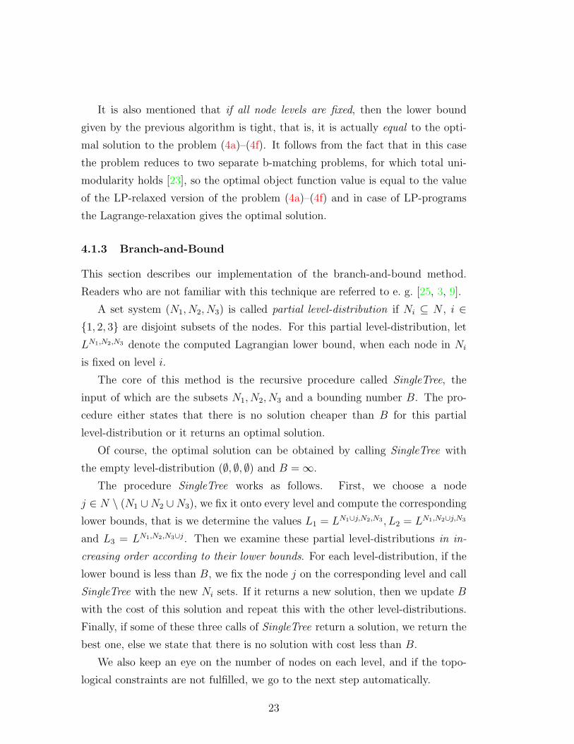
4.1.3 Branch-and-Bound

This section describes our implementation of the branch-and-bound method.

Readers who are not familiar with this technique are referred to e. g. [25, 3, 9].

A set system (N1, N2, N3) is called partial level-distribution if Ni ⊆ N , i ∈{1, 2, 3} are disjoint subsets of the nodes. For this partial level-distribution, let

LN1,N2,N3 denote the computed Lagrangian lower bound, when each node in Ni

is fixed on level i.

The core of this method is the recursive procedure called SingleTree, the

input of which are the subsets N1, N2, N3 and a bounding number B. The pro-

cedure either states that there is no solution cheaper than B for this partial

level-distribution or it returns an optimal solution.

Of course, the optimal solution can be obtained by calling SingleTree with

the empty level-distribution (∅, ∅, ∅) and B = ∞.

The procedure SingleTree works as follows. First, we choose a node

j ∈ N \ (N1 ∪N2 ∪N3), we fix it onto every level and compute the corresponding

lower bounds, that is we determine the values L1 = LN1∪j,N2,N3 , L2 = LN1,N2∪j,N3

and L3 = LN1,N2,N3∪j. Then we examine these partial level-distributions in in-

creasing order according to their lower bounds. For each level-distribution, if the

lower bound is less than B, we fix the node j on the corresponding level and call

SingleTree with the new Ni sets. If it returns a new solution, then we update B

with the cost of this solution and repeat this with the other level-distributions.

Finally, if some of these three calls of SingleTree return a solution, we return the

best one, else we state that there is no solution with cost less than B.

We also keep an eye on the number of nodes on each level, and if the topo-

logical constraints are not fulfilled, we go to the next step automatically.

23

An easy modification of this method enables to give an approximation algo-

rithm to our problem. The idea is to skip a possible partial fixing not only if

the lower bound is worse than the best solution but also if they are close enough

to each other. Namely an error factor err is introduced and a partial fixing is

examined only if the corresponding lower bound is less than 11+err

B. This ensures

that the resulted solution is worse at most by the factor err than the optimum.

function SingleTree(N1, N2, N3, B)

{if (2 · |N1| < |N2| or 2 · |N2| < |N3|) then return ∞else {

if (N = N1 ∪N2 ∪N3) then return LN1,N2,N3

else {j ∈ N \ (N1 ∪N2 ∪N3)

C1 := (N1 + j, N2, N3)

C2 := (N1, N2 + j, N3)

C3 := (N1, N2, N3 + j)

L1 := LC1 , L2 := LC2 , L3 := LC3

((L′1, C

′1), (L

′2, C

′2), (L

′3, C

′3)) := sort-by-L((L1, C1), (L2, C2), (L3, C3))

B∗ := B

if (L′3 < B∗) then B∗ = min{B∗,SingleTree(C ′

3, B∗)}

if (L′2 < B∗) then B∗ = min{B∗,SingleTree(C ′

2, B∗)}

if (L′1 < B∗) then B∗ = min{B∗,SingleTree(C ′

1, B∗)}

if (B∗ < B) then return B∗

else return ∞}

}}

Figure 4: The SingleTree algorithm

24

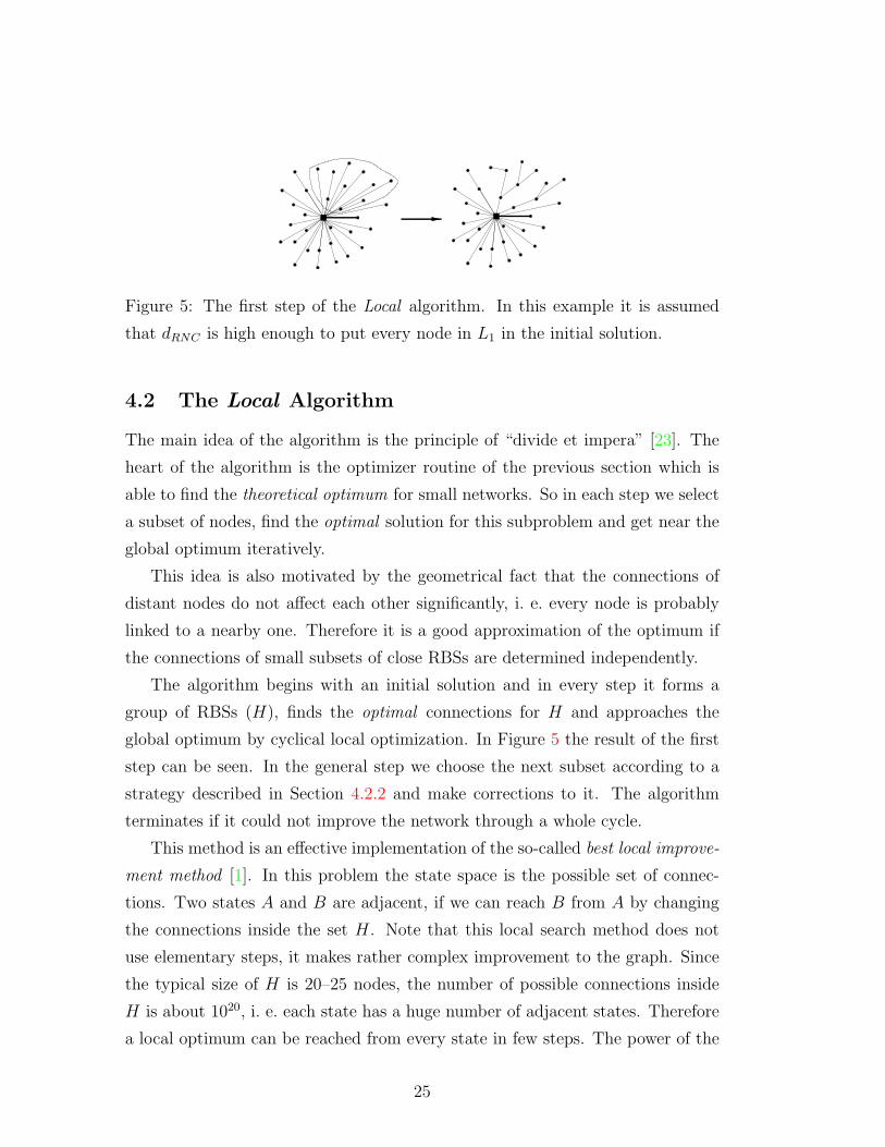
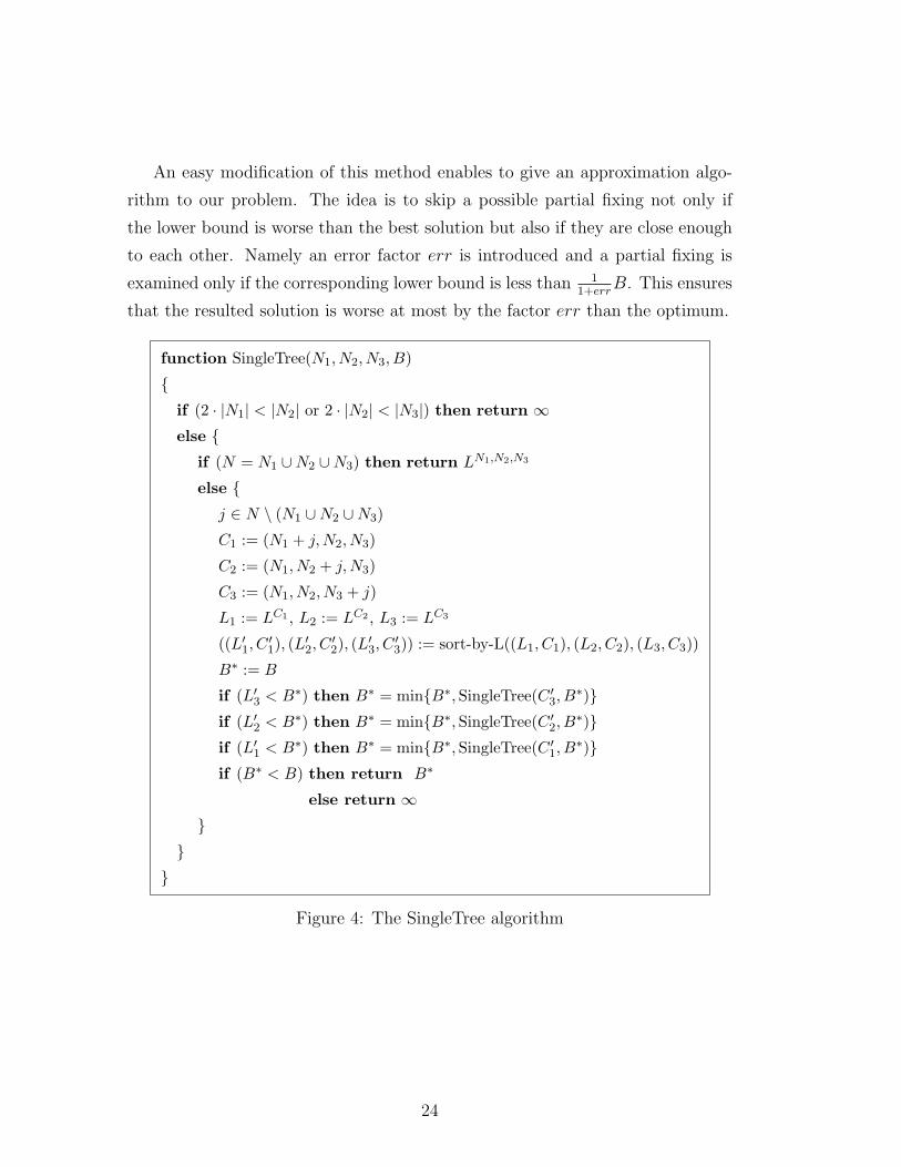
Figure 5: The first step of the Local algorithm. In this example it is assumed

that dRNC is high enough to put every node in L1 in the initial solution.

4.2 The Local Algorithm

The main idea of the algorithm is the principle of “divide et impera” [23]. The

heart of the algorithm is the optimizer routine of the previous section which is

able to find the theoretical optimum for small networks. So in each step we select

a subset of nodes, find the optimal solution for this subproblem and get near the

global optimum iteratively.

This idea is also motivated by the geometrical fact that the connections of

distant nodes do not affect each other significantly, i. e. every node is probably

linked to a nearby one. Therefore it is a good approximation of the optimum if

the connections of small subsets of close RBSs are determined independently.

The algorithm begins with an initial solution and in every step it forms a

group of RBSs (H), finds the optimal connections for H and approaches the

global optimum by cyclical local optimization. In Figure 5 the result of the first

step can be seen. In the general step we choose the next subset according to a

strategy described in Section 4.2.2 and make corrections to it. The algorithm

terminates if it could not improve the network through a whole cycle.

This method is an effective implementation of the so-called best local improve-

ment method [1]. In this problem the state space is the possible set of connec-

tions. Two states A and B are adjacent, if we can reach B from A by changing

the connections inside the set H. Note that this local search method does not

use elementary steps, it makes rather complex improvement to the graph. Since

the typical size of H is 20–25 nodes, the number of possible connections inside

H is about 1020, i. e. each state has a huge number of adjacent states. Therefore

a local optimum can be reached from every state in few steps. The power of the

25

algorithm is that in spite of the large number of neighbors the optimizer function

chooses the best one in each step.

4.2.1 Finding an Initial Solution

The algorithm can be utilized to improve the solution given by a previous one,

hence in this case the starting solution is given. However, the algorithm can

also work independently, so it should be capable of finding an initial solution

satisfying the conditions.

• The easiest way to do that is to put dRNC randomly chosen RBSs in the set

L1, dRNC · dRBS randomly chosen ones in set L2, etc. This trivial solution

satisfies the constraints.

• A more sophisticated way to find an initial solution is the following: as

described in Section 4.1.3 the core optimizer can be configured to return

the theoretical optimum or work with a predefined error rate (err). If err is

high enough, the optimization becomes very fast, but of course less effective.

So by setting the error rate high in the first cycle (i. e. until every RBS is at

least once picked in H) we could quickly find a considerably better starting

solution than the previously mentioned trivial one.

4.2.2 Selection of H

In each step of the algorithm a new set H is selected and given as input for the

optimizer. On the one hand, H should consist of close RBSs, on the other hand,

it should contain whole subtrees only2, each rooting in a first level RBS. This is

important because during optimization the connections in H will be changed, so

otherwise it would be possible to make unconnected RBSs.

To satisfy these conditions we select adjacent subtrees of the current network

rooting in a first-level node until a predefined upper bound (hmax) for the size of

H has been reached. The first-level RBSs are ordered according to their location

(clockwise around the RNC). An example for such a selection can be seen in

2Of course the RNC is always in H.

26

3

7

2

4

5

6

1

Figure 6: The selection of H

n TreePlan Global IterationGlobal

Global+LocalGlobal+Local

vs. TreePlan vs. TreePlan

100 4736 4363 19880 7.9% 4168 12.0%

200 9048 8757 20905 3.2% 8485 6.2%

300 13534 13274 20879 2.0% 12747 5.8%

400 18389 18040 19439 1.9% 17005 7.5%

500 23037 21943 22772 4.7% 21293 7.6%

600 27533 26662 29872 3.2% 25759 6.4%

1000 45686 43916 28596 3.9% 42645 6.7%

Table 2: Results of the algorithms (with dRNC = ∞) compared with TreePlan.

Figure 6. The selection starts in every step with another first-level node, which

guarantees the variety of H.

Since the core optimizer solves anNP-hard problem, its speed is very sensitive

to the size of its input, i. e. |H|. Choosing the parameter hmax at the beginning

of the algorithm, we can set an upper bound for |H|. Of course the higher |H|is, the better the result will be, but the slower the algorithm becomes.

5 Numerical Results

In our empirical tests we used the TreePlan algorithm [12, 13] as a reference

method since to our knowledge this is the only method in the literature that is

27

able to solve problems similar to ours.

First the Global algorithm was executed on several test cases, then in a second

phase the Local algorithm was used to improve the results of the Global algorithm.

(Note that the Local algorithm can also be used to re-design the trees of any

planning algorithms, e. g. the Global algorithm.) Both results were compared

with TreePlan.

Although our algorithms can work with arbitrary parameters, the values

dRBS = 2 and ltree = 3 are fixed in our test cases, for these values are cur-

rently accepted in the UMTS architecture. The cost of an RNC node, costRNC

was set to 500 during all tests, and length proportional link cost function was

used. In order to be able to compare the numerical results to those of TreePlan,

dRNC was set to ∞ in the comparative test cases. After these we present some

tests on the Global algorithm with different dRNC values.

The Global algorithm terminates if there is no new state accepted during a

predefined number of iterations (K) in the simulated annealing. This frees the

tester to explicitly set the number of iterations in the simulated annealing for

different initial temperature and decreasing factor values. In the following results

the decreasing factor fact was set to 0.9995, the initial temperature T0 was 20000

and K was set to 2000.

The results of our tests can be seen in Table 2. The first column is the size of

n dRNC Cost Time

700 100 30658 21m03s

700 50 30658 18m38s

700 25 30737 18m37s

700 10 31506 19m24s

700 5 36956 17m16s

700 3 45263 15m13s

700 2 56437 14m21s

700 1 80860 15m25s

Table 3: Results of the Global algorithm with different dRNC values.

28

the network, then the total network cost planned by TreePlan and by the Global

algorithm is compared. The fourth column contains the number of iterations

made by the Global algorithm. In the sixth column the improvement of the Local

algorithm on the Global algorithm can be seen, and finally the total improvement

vs. TreePlan.

In all of the test cases the Global algorithm alone can reduce the cost of

the UMTS network; moreover the Local algorithm was able to make further

improvements on the trees in every test. The size of these trees varied from 35 to

200, showing that the Local algorithm is appropriate for practical sized problems.

As we expected the best results can be found by the combination of the two new

methods, which gave an improvement of 6-7%, in extreme cases even of 12%

compared to the former approach, TreePlan.

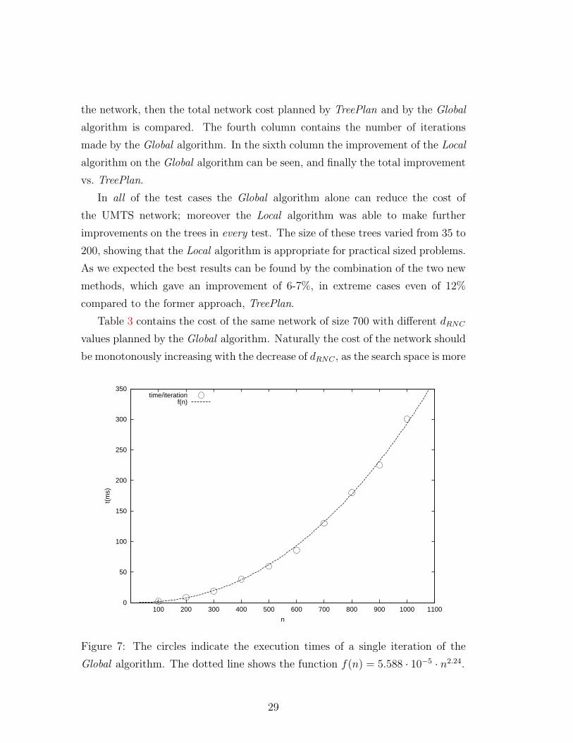
Table 3 contains the cost of the same network of size 700 with different dRNC

values planned by the Global algorithm. Naturally the cost of the network should

be monotonously increasing with the decrease of dRNC , as the search space is more

0

50

100

150

200

250

300

350

100 200 300 400 500 600 700 800 900 1000 1100

t(m

s)

n

time/iterationf(n)

Figure 7: The circles indicate the execution times of a single iteration of the

Global algorithm. The dotted line shows the function f(n) = 5.588 · 10−5 · n2.24.

29

constrained. The results clearly reflect this characteristic.

The execution times of the Global algorithm on a 400MHz PC under SuSe

Linux 7.1 can be seen in Figure 7. (On the x axis the number of nodes, on

the y axis the execution time of an iteration in milliseconds can be seen.) The

figure indicates that the running time is approx. O(n2.24). Since the b-matching

algorithm is an O(n3) method, the acceleration of the algorithm in Section 3.2.3

is significant. Note that just scanning the input requires O(n2) time.

The number of iterations highly depends on the initial parameters and the

termination criterion of the Simulated Annealing. In case of the above tests the

number of iterations was in the range of 20-30.000. Of course, our algorithms are

slower than the former approach according to the more complex computation.

However, in a typical network design process one would run the planning algo-

rithm a couple of times only, hence an execution time of about 2.5 hours for a

network with 1000 nodes (which is the size of usual UMTS networks) should be

acceptable.

We also tested the Local algorithm separately. The subgradient method ap-

plied in the tests was as in e. g. [9]. Our objective was to estimate the difference

of the results of the Local algorithm and the optimum. Therefore we calculated

the lower bound of several test instances as described in Section 4.1.2 and com-

pared it to the result of the Local algorithm. We considered 4 problem sizes each

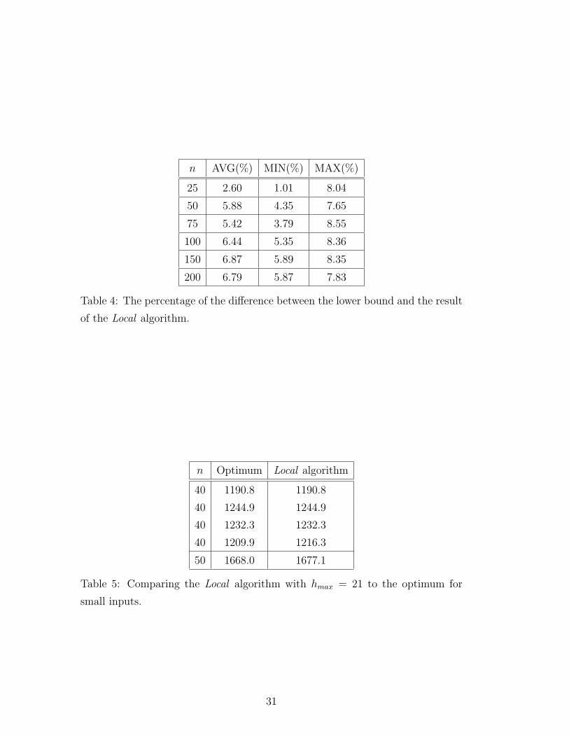
with 10 different networks. Table 4 presents the average/minimum/maximum

difference between the lower bound and the Local algorithm with hmax = 24.

This means, that the Local algorithm gives around 5-7% approximation of the

optimum value in average for practical examples of 25-200 nodes.

Following test shows, that in small problems the actual difference is even

smaller. Namely one may sets hmax to n to get the global optimum. This is of

course feasible for smaller n values only. Table 5 shows the results of comparing

the Local algorithm with hmax = 21 with the optimum value—also computed

with the Local algorithm with hmax = n. The table shows 4 different networks

with 40 nodes and one network with 50 nodes. One can clearly see that for small

inputs the Local algorithm gives almost always optimum.

The local algorithm can also handle the dRNC constraint, however this has

only theoretical importance. Since the input of the Local algorithm is only one

30

n AVG(%) MIN(%) MAX(%)

25 2.60 1.01 8.04

50 5.88 4.35 7.65

75 5.42 3.79 8.55

100 6.44 5.35 8.36

150 6.87 5.89 8.35

200 6.79 5.87 7.83

Table 4: The percentage of the difference between the lower bound and the result

of the Local algorithm.

n Optimum Local algorithm

40 1190.8 1190.8

40 1244.9 1244.9

40 1232.3 1232.3

40 1209.9 1216.3

50 1668.0 1677.1

Table 5: Comparing the Local algorithm with hmax = 21 to the optimum for

small inputs.

31

RNC, the

dRNC ≥

⌈n∑ltree−1

i=0 diRBS

⌉must hold (here the denominator equals to the maximum number of nodes in a

subtree rooting in a first-level node). The Local algorithm without an RNC degree

constraint plans a network with RNC degree just slightly above the lower bound.

For instance in a network of 100 nodes (with dRBS = 2, ltree = 3) dRNC ≥ 15

must hold, and the Local algorithm without any RNC degree constraint returns

a network with RNC degree equals to 16.

6 Conclusion

In this paper two new algorithms were introduced for planning UMTS access

networks. The first one — relying on a combination of the Simulated Anneal-

ing heuristic and a specific b-matching problem — plans global UMTS access

networks, the second one — which uses Lagrangian lower bound with branch-

and-bound — is able to plan a single tree or make corrections to existing UMTS

trees. It has been also demonstrated by a number of test cases how these methods

can reduce the total cost of UMTS networks.

Nevertheless, some basic simplifications concerning the capacity dependent

part of the cost functions were proposed. The more proper consideration of this

cost factor of UMTS access networks is the next direction of further research.

7 Acknowledgments

The authors would like to thank to Zoltan Kiraly for his useful ideas and also to

Tibor Cinkler, Andras Frank, Gabor Magyar, Aron Szentesi, Balazs Szviatovszki

and the anonymous referees for their valuable suggestions and comments.

A NP-hardness of the single-tree problem

Claim A.1 Let G(V, E) denote an undirected connected complete graph, RNC ∈V be a given vertex, and dRNC ∈ N+. Moreover we are given the function c : E →

32

R+ determining the cost of the edges. Then the problem of finding a minimal cost

spanning tree with the following properties is NP-hard:

• every node can be reached from the RNC in a path of length at most 3,

• every node except the RNC has degree at most 3,

• RNC has degree at most dRNC.

Proof. We show a Karp-reduction of the well-known NP-complete 3–uniform

set covering problem (referred as Problem [SP5] in [10]) to this one. The input

of the 3–uniform set covering problem is an integer number l and a class of sets

H := {X1, X2, · · · , Xn} over an underlining set H (|H| ≥ 3), such that

Xi ⊆ H, |Xi| = 3 ∀i ∈ {1, ..., n}

andn⋃

i=1

Xi = H.

The problem is to determine whether there exist at most l sets in H still

covering H.

This problem is reduced to the following single-tree problem. First, |H|nodes are defined corresponding the elements of H and six additional nodes

ai, bi, ci, di, ei, fi are defined for each element Xi of H. Moreover, an RNC node

is also defined.

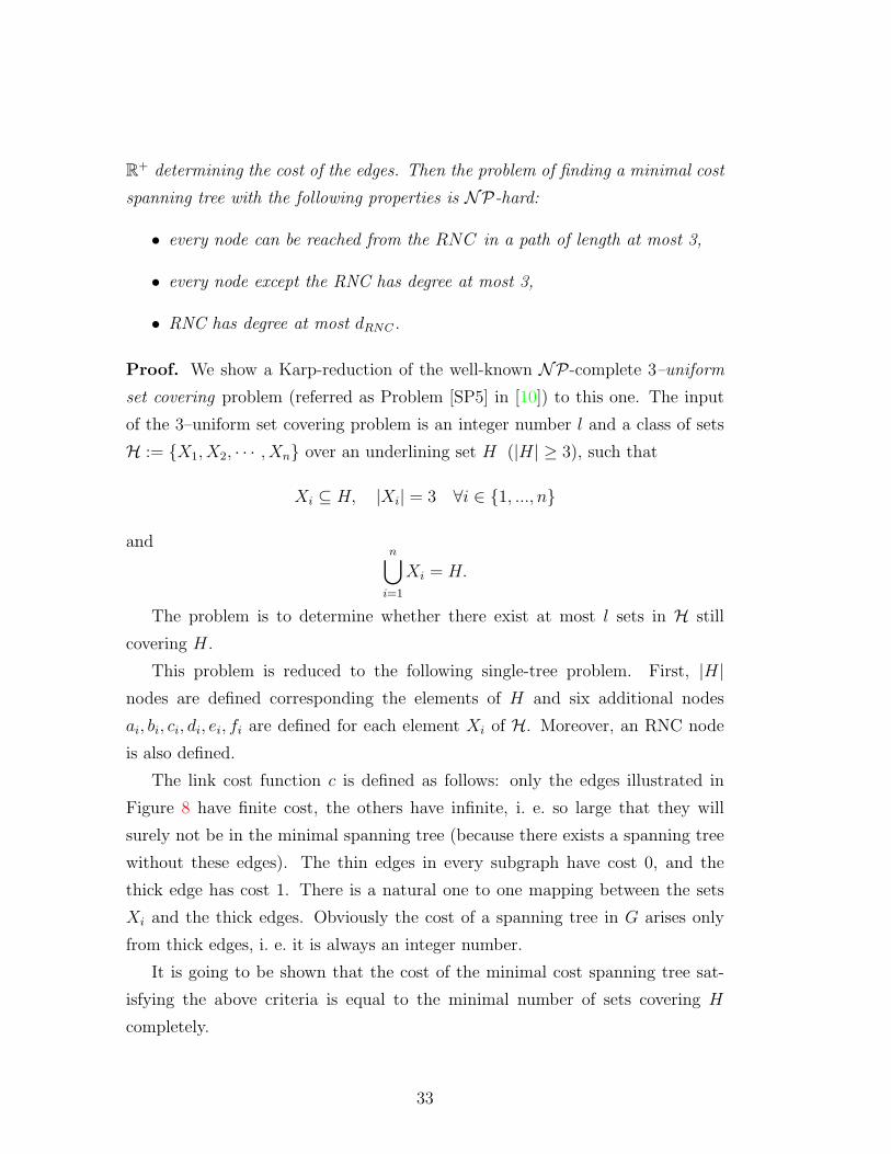
The link cost function c is defined as follows: only the edges illustrated in

Figure 8 have finite cost, the others have infinite, i. e. so large that they will

surely not be in the minimal spanning tree (because there exists a spanning tree

without these edges). The thin edges in every subgraph have cost 0, and the

thick edge has cost 1. There is a natural one to one mapping between the sets

Xi and the thick edges. Obviously the cost of a spanning tree in G arises only

from thick edges, i. e. it is always an integer number.

It is going to be shown that the cost of the minimal cost spanning tree sat-

isfying the above criteria is equal to the minimal number of sets covering H

completely.

33

ai ci

e i

f i

bi di

1

Xi

H

RNC

Figure 8: The subgraph associated with each set Xi

ai ci

di

e i

f i

bi

RNC

Xi

H

(a) The part of the spanning tree be-

longing to the Xi sets not in the min-

imal covering set. The cost is 0.

ai ci

di

e i

f i

bi

RNC

1

Xi

H

(b) The part of the spanning tree be-

longing to the Xi sets in the minimal

covering set. The cost is 1.

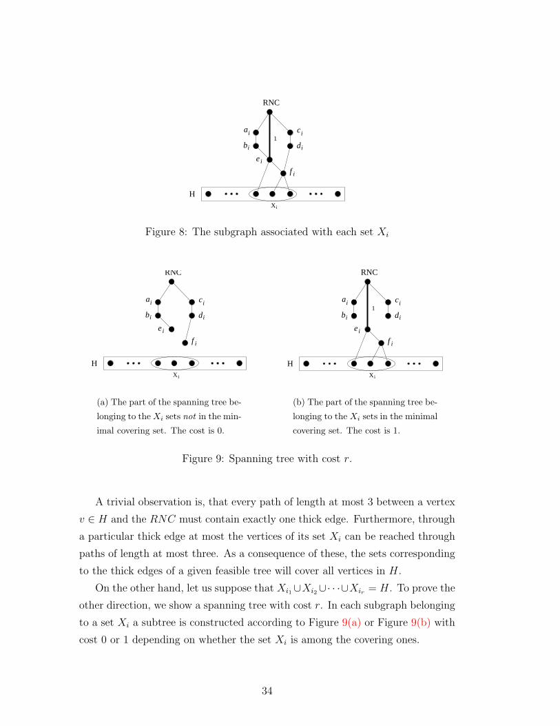
Figure 9: Spanning tree with cost r.

A trivial observation is, that every path of length at most 3 between a vertex

v ∈ H and the RNC must contain exactly one thick edge. Furthermore, through

a particular thick edge at most the vertices of its set Xi can be reached through

paths of length at most three. As a consequence of these, the sets corresponding

to the thick edges of a given feasible tree will cover all vertices in H.

On the other hand, let us suppose that Xi1∪Xi2∪· · ·∪Xir = H. To prove the

other direction, we show a spanning tree with cost r. In each subgraph belonging

to a set Xi a subtree is constructed according to Figure 9(a) or Figure 9(b) with

cost 0 or 1 depending on whether the set Xi is among the covering ones.

34

The union of these subtrees covers every vertex in G, since the covering set

covers every vertex in H and the V \ H vertices are covered by the subtrees

in both cases. It may happens that this union contains cycles, but by simply

neglecting the superfluous edges a spanning tree is obtained with cost at most r.

�

References

[1] Emile Aarts, Jan Karel Lenstra Local Search in Combinatorial Optimization,

John Wiley & Sons, Inc., 1997.

[2] N. R. Achuthan, L. Caccetta, J. F. Geelen, Algorithms for the minimum

weight spanning tree with bounded diameter problem, Optimization: Tech-

niques and Applications (1992) pp. 297-304.

[3] Ravindra K. Ahuja, Thomas L. Magnanti, James B. Orlin: Network Flows,

PRENTICE HALL,1993

[4] Mokhtar S. Bazaraa, Hanif D. Sherali, C. M. Shetty, Nonlinear Programming

- Theory and Algorithms, John Wiley & Sons, Inc. 1993.

[5] P. Chardaire, Upper and lower bounds for the two-level simple plant location

problem, Annals of Operations Research, 1998.

[6] Joseph C. S. Cheung, Mark A. Beach, Joseph P. McGeehan, Network Plan-

ning for Third-Generaion Mobile Radio Systems, IEEE Communication

Magazine, November 1994

[7] W.J. Cook, W. H. Cunningham, W. Puleyblank, A. Schrijver, Combina-

torial Optimization, Wiley-Interscience Series in Discrete Matehematics and

Optimization

[8] ILOG CPLEX 7.1 User’s Manual, ILOG, 2001.

[9] Mark S. Daskin Network and Discrete Location, Jon Wiley and Sons Inc.,

1995.

35

[10] M. R. Garey, D. S. Johnson, Computers and Intractability — A Guide to

the Theory of NP-Completeness, W. H. Freeman and Company, New York,

1979.

[11] F. Glover: Tabu Search - part I and II, ORSA Journal on Computing 1(3),

1989 and 2(1), 1990.

[12] Janos Harmatos, Alpar Juttner, Aron Szentesi: Cost-Based UMTS Transport

Network Topology Optimization, ICCC 99, Japan, Tokyo, Sept 1999

[13] Janos Harmatos, Aron Szentesi, Istvan Godor: Planning of Tree-Topology

UMTS Terrestrial Access Networks, PIMRC 2000, England, London, Sept

18-21

[14] Paul Kallenberg, Optimization of the Fixed Part GSM Networks Using Sim-

ulated Annealing, Networks 98, Sorrento, October 1998.

[15] S.Kirkpatrick, C.D. Gelatt, JR., M.P. Vecchi, Optimization by simulated

annealing, Science 220:671-680 1983.

[16] J. G. Klincewicz, Hub location in backbone/tributary network design: a re-

view, Location Science 6 (1998) pp.307-335.

[17] N. Deo, N. Kumar, Constrained spanning tree problems: Approximate meth-

ods and parallel computation in Network Design: Connectivity and Facilities

Location, DIMACS Workshop April 28-30, 1997, pp. 191–219

[18] N. Deo, N. Kumar, Computation of Constrained Spanning Trees: A Unified

Approach in Network Optimization, edited by P. M. Pardalos, D. W. Hearn,

W. W. Hager, Springer-Verlag, 1997

[19] Facility Location: A Survey of Applications and Methods, edited by Zvi

Drezner, Springer-Verlag, 1995.

[20] Brian G. Marchent, Third Generation Mobile Systems for the Support of

Mobile Multimedia based on ATM Transport, tutorial presentation, 5th IFIP

Workshop, Ilkley, July 1997.

36

[21] Tero Ojanpera, Ramjee Prasad, Wideband CDMA for Third Generation Mo-

bile Communication, 1998, Artech House Publishers.

[22] G. M. Schneider, Mary N. Zastrow, An Algorithm for Design of Multilevel

Concentrator Networks, Computer Networks 6 (1982) pp. 1-11.

[23] Alexander Schrijver, Theory of Linear and Integer Programming, John Wi-

ley & Sons, Inc, 1998

[24] The Path towards UMTS - Technologies for the Information Society, UMTS

Forum, 1998

[25] Laurence A. Wolsey, Integer Programming John Wiley & Sons, Inc, 1998.

37