Two-level logic minimization: an overview

Olivier Coudert

DEC, Paris Research Laboratory,85 Avenue Victor Hugo,

92500 Rueil Malmaison, France

INTEGRATION, the VLSI journal, 17-2, pp. 97–140, October 1994.

Contents

1 Introduction 5

2 Minimization over a product space 62.1 Product space and Boolean functions . . . . . . . . . . . . . . . . . . . . . . . . . . . . . 62.2 Implicants, primality, essentiality . . . . . . . . . . . . . . . . . . . . . . . . . . . . . . . 82.3 Example . . . . . . . . . . . . . . . . . . . . . . . . . . . . . . . . . . . . . . . . . . . . . 92.4 Set covering problem . . . . . . . . . . . . . . . . . . . . . . . . . . . . . . . . . . . . . . 10

3 The Quine–McCluskey procedure 103.1 Prime implicant computation . . . . . . . . . . . . . . . . . . . . . . . . . . . . . . . . . 113.2 Reduction processes . . . . . . . . . . . . . . . . . . . . . . . . . . . . . . . . . . . . . . 12

3.2.1 Partitioning . . . . . . . . . . . . . . . . . . . . . . . . . . . . . . . . . . . . . . . 123.2.2 Essentiality . . . . . . . . . . . . . . . . . . . . . . . . . . . . . . . . . . . . . . . 123.2.3 Dominance relations . . . . . . . . . . . . . . . . . . . . . . . . . . . . . . . . . . 123.2.4 Gimpel’s reduction . . . . . . . . . . . . . . . . . . . . . . . . . . . . . . . . . . . 13

3.3 Branch and bound . . . . . . . . . . . . . . . . . . . . . . . . . . . . . . . . . . . . . . . 143.3.1 Branching . . . . . . . . . . . . . . . . . . . . . . . . . . . . . . . . . . . . . . . . 153.3.2 Lower bound . . . . . . . . . . . . . . . . . . . . . . . . . . . . . . . . . . . . . . 15

3.4 Conclusion . . . . . . . . . . . . . . . . . . . . . . . . . . . . . . . . . . . . . . . . . . . 15

4 Formalizing covering matrix reduction 164.1 Strong reduction with dominance relations . . . . . . . . . . . . . . . . . . . . . . . . . . 164.2 Transposing functions . . . . . . . . . . . . . . . . . . . . . . . . . . . . . . . . . . . . . 174.3 Conclusion . . . . . . . . . . . . . . . . . . . . . . . . . . . . . . . . . . . . . . . . . . . 19

5 The signature cube based procedure 19

6 Set covering problem over lattices 216.1 Lattices . . . . . . . . . . . . . . . . . . . . . . . . . . . . . . . . . . . . . . . . . . . . . 226.2 Solving set covering problems over a lattice . . . . . . . . . . . . . . . . . . . . . . . . . 22

6.2.1 Examples and intuition . . . . . . . . . . . . . . . . . . . . . . . . . . . . . . . . 22

1

6.2.2 The transposing function τW,⊑ . . . . . . . . . . . . . . . . . . . . . . . . . . . . 246.2.3 Essential elements . . . . . . . . . . . . . . . . . . . . . . . . . . . . . . . . . . . 256.2.4 Recovering the original solutions . . . . . . . . . . . . . . . . . . . . . . . . . . . 25

7 A new two-level logic minimization procedure 267.1 Implicit prime implicant computation . . . . . . . . . . . . . . . . . . . . . . . . . . . . 277.2 Computing Q . . . . . . . . . . . . . . . . . . . . . . . . . . . . . . . . . . . . . . . . . . 287.3 Computing max⊆ τP (Q) . . . . . . . . . . . . . . . . . . . . . . . . . . . . . . . . . . . . 287.4 Computing max⊆ τQ(P ) . . . . . . . . . . . . . . . . . . . . . . . . . . . . . . . . . . . . 297.5 Improvements for solving the covering matrix . . . . . . . . . . . . . . . . . . . . . . . . 30

7.5.1 Pruning with the left-hand side lower bound . . . . . . . . . . . . . . . . . . . . 317.5.2 The limit lower bound theorem . . . . . . . . . . . . . . . . . . . . . . . . . . . . 31

7.6 Conclusion . . . . . . . . . . . . . . . . . . . . . . . . . . . . . . . . . . . . . . . . . . . 32

8 Experimental results 32

9 Conclusion 35

A Binary Decision Diagrams 35

B Combinational sets 37

Bibliographie 39

List of Figures

1 A total Boolean function on 0, 13 and its associated on-set. . . . . . . . . . . . . . . . 72 Karnaugh map. . . . . . . . . . . . . . . . . . . . . . . . . . . . . . . . . . . . . . . . . . 93 Karnaugh maps of an irredundant and two minimal prime covers. . . . . . . . . . . . . . 104 A covering matrix. . . . . . . . . . . . . . . . . . . . . . . . . . . . . . . . . . . . . . . . 115 Reduction by essentiality. . . . . . . . . . . . . . . . . . . . . . . . . . . . . . . . . . . . 126 Reduction by domination on X. . . . . . . . . . . . . . . . . . . . . . . . . . . . . . . . . 137 Reduction by domination on Y . . . . . . . . . . . . . . . . . . . . . . . . . . . . . . . . . 138 Gimpel’s reduction on x. . . . . . . . . . . . . . . . . . . . . . . . . . . . . . . . . . . . . 149 Strong dominance reduction with equivalence classes. . . . . . . . . . . . . . . . . . . . . 1710 Universal transposing functions based reduction. . . . . . . . . . . . . . . . . . . . . . . 1911 Signature cubes and minterm dominance. . . . . . . . . . . . . . . . . . . . . . . . . . . 2012 Naive computation of max⊆ σ(f). . . . . . . . . . . . . . . . . . . . . . . . . . . . . . . . 2113 Computing τX,⊑(Y ) on a lattice. . . . . . . . . . . . . . . . . . . . . . . . . . . . . . . . 2314 Computing τY,⊒(X) on a lattice. . . . . . . . . . . . . . . . . . . . . . . . . . . . . . . . 2315 Computing the essential elements. . . . . . . . . . . . . . . . . . . . . . . . . . . . . . . 2416 Algorithm Prime. . . . . . . . . . . . . . . . . . . . . . . . . . . . . . . . . . . . . . . . 2817 DiveMinIntoP. . . . . . . . . . . . . . . . . . . . . . . . . . . . . . . . . . . . . . . . . . 2818 Algorithm NotSubSet. . . . . . . . . . . . . . . . . . . . . . . . . . . . . . . . . . . . . . 2919 Algorithm MaxTauP . . . . . . . . . . . . . . . . . . . . . . . . . . . . . . . . . . . . . . 2920 Algorithm SupSet. . . . . . . . . . . . . . . . . . . . . . . . . . . . . . . . . . . . . . . . 2921 Algorithm MaxTauQ. . . . . . . . . . . . . . . . . . . . . . . . . . . . . . . . . . . . . . 30

2

22 Espresso-Exact, Espresso-Signature, and Scherzo. . . . . . . . . . . . . . . . . . . . . . . 3423 Shannon tree and BDD of the function x1(x3 ⊕ x4) + x2(x3 ⇔ x4). . . . . . . . . . . . . 3624 Reduction rules rewriting a Shannon tree into a BDD. . . . . . . . . . . . . . . . . . . . 3625 Reduction rules rewriting a set of sparse combinations into a CS. . . . . . . . . . . . . . 3826 CS of the set of products bd, abcd, acd. . . . . . . . . . . . . . . . . . . . . . . . . . . . 39

List of Tables

1 Computation time for 33 examples . . . . . . . . . . . . . . . . . . . . . . . . . . . . . . 442 The hard Espresso-Exact problems . . . . . . . . . . . . . . . . . . . . . . . . . . . . . . 453 Hard espresso examples with Espresso-Signature and Scherzo . . . . . . . . . . . . . . . 464 Results of Scherzo on hard examples from the MIS and ISCAS benchmarks . . . . . . . 47

Notation

X,Y, Z, . . . Sets.x, y, z, . . . Elements of a set.∪,∩,−,× Union, intersection, set difference, cartesian product.f Function.f−1 Inverse function of f .2S Power set of a set S.f(S) Image of a function f on a set S.i, j, k, n,m Integers, indices.· Ordered cartesian product.L Product space, i.e., set

∏

k Lk = L1 · L2 · · · ·.lk Literal, i.e., subset of a set Lk.∏

k lk Product built on a product space L.P(L) Set of all products built on a a product space L.P,Q Sets of products.p, q, r Products.Plk Set of products p | lk · p ∈ P.B The particular product space 0, 1n.minterm An element of B.a, b, c, d, x, xk Boolean variables and positive literals.x Negation of the Boolean variable x, negative literal.abcd, x1x2 Products built on B.P1k , Pxk

, PxkCanonical decomposition of a set of products built on B.

f1 On-set of a partial boolean function f .f1∗ Union of the on-set and the don’t care set of f .flk Largest set such that lk · flk ⊆ f .fx, fx Shannon expansion of the Boolean function f w.r.t a Boolean variable x.Prime(f) Set of prime implicants of f .X,Y Set of rows and set of columns.x, x′, y, y′ Rows and columns.Cost(y) Cost of a column.R Subset of X × Y .

3

〈X,Y,R〉 Set covering problem.E Set of essential columns.Sol(C) Set of minimal solution of a set covering problem C.≺ Quasi order., ⊑ Partial order.≡ Equivalence relation.π Map an element onto its equivalence class.ρ Map an equivalence class onto one of its element.→ Rewriting rule, mapping.Z/≡ Quotient set of Z by an equivalence relation ≡.≺Y Dominance relation on rows.≺X Dominance relation on columns.max Maximal elements of a set w.r.t. a quasi or partial order.τ Transposing function.σ(x) Signature cube of a minterm x.(Z,⊑) Lattice.sup Least upper bound of a set.inf Greatest lower bound of a set.⊗ Inner product, i.e., P ⊗Q = p · q | p ∈ P, q ∈ Q.

4

Two-level logic minimization: an overview

INTEGRATION, the VLSI journal, 17-2, pp. 97–140, October 1994.

Olivier Coudert

Abstract

Fourty years ago Quine noted that finding a procedure that computes a minimal sum of productsfor a given propositional formula is very complex, even though propositional formulas are fairlysimple. Since this early work, this problem, known as two-level logic minimization, has attractedmuch attention. It arises in several fields of computer science, e.g., in logic synthesis, reliabilityanalysis, and automated reasoning. This paper exposes the classical approach for two-level logicminimization, and presents the recent developments that overcome the limitations of the proceduresproposed in the past. We show that these new techniques yield a minimizer that is 10 up to 50 timesfaster than the previously best known ones, and that is able to handle more complex functions.

Keyword

Set covering problem, Two-level logic minimization, Binary Decision Diagram, Combinational Set,Transposing function

1 Introduction

In 1952, Quine observed that finding a procedure that reduces propositional formulas to their “smallest”equivalent forms is complex, even though Propositional Logic is quite “simple” [45]. Quine was interestedin propositional formulas represented in disjunctive normal form. A disjunctive normal form, also calledsum-of-products, is a disjunction of products. A product is a conjunction of literals (each literal isa propositional variable or its negation). For instance, a and b are literals, abc is a product, andabc + acd + bd is a sum-of-products. The problem is to find, given a Boolean function f , the minimalsum-of-products that represents f . This problem is known as two-level logic minimization.

Consider the following sum-of-products:

abd+ acd+ abcd+ abc+ acd+ bcd.

A simpler equivalent sum-of-products can be found by merging some products, or by removing someliterals from some products. For instance, abd logically implies acd + bcd (one says that acd + bcdcontains abd), thus abd can be removed from the expression. Also acd contains the minterm abcd, sothe product abcd in the original expression can be replaced with bcd. We then obtain:

acd+ abc+ acd+ bcd+ bcd.

5

At this step we can neither remove any product from this sum-of-products, nor a literal from anyproduct, without modifying the function the original expression represents. This sum-of-products islocally minimal, or irredundant. However there are smaller sums-of-products. Indeed,

acd+ abd+ bcd+ bcd and abd+ abc+ abc+ acd

are the two absolute minimal sums-of-products representations of the original expression. Note that inthese two minimal sums-of-products, some products do not occur in the original expression, e.g., abcand bcd, even as subexpressions, e.g., abd.

Computing an irredundant or minimal sum-of-products has several applications in computer sci-ence. In logic synthesis a minimal sum-of-products provides the user with an efficient implementationof a single or multi-output Boolean functions with NOT, AND and OR gates [26, 6, 55]. In reliabilityanalysis, a sum-of-products is a way for either exhaustively, or concisely, representing the causes offailure of a system [25, 18]. In automated reasoning, a sum-of-products can be either a set of minimaldemonstrations, or the normalization of a formula into a disjunctive normal form for further computa-tions [22, 30, 31, 49, 50, 39].

Since Quine established the problem of computing minimal sums-of-products in the 1950’s [45],efforts have been made to discover efficient minimization procedures [48, 34, 3, 26, 6, 56, 57, 37, 27].These procedure encounter two bottlenecks. The first one is the number of prime implicants theyhave to generate, the second one is that solving a set covering problem is itself NP-hard. Most of theprocedures proposed in the past are limited by huge numbers of products one has to manipulate forsome functions, typically their number of prime implicants. This paper shows how recent developmentsyield new techniques for computing minimal sum-of-products, whose complexities no longer depend onthe numbers of products to manipulate.

This paper aims at presenting the standart techniques used to compute a minimal cost sum-of-products representation of a given Boolean function, as well as the last recent developments in this field.Section 2 defines the two-level minimization problem in the more general terms of a paving problem,and explains some useful notions such as implicants, primality, essentiality, and set covering problems.Section 3 presents the well known Quine–McCluskey algorithm that is widely used for two-level logicminimization. Section 4 formalizes the concept of dominance relation used by the Quine–McCluskeyalgorithm and introduces the notion of transposing function. Section 5 presents the signature cube basedminimization method that is a direct consequence of the results derived in Section 4. Section 6 addressesthe resolution of a generic set covering problem, namely set covering problem over a lattice, and presentsan original minimization algorithm. Section 7 is a direct application of the results introduced in Section6 to two-level logic minimization. Section 8 presents and discusses some experimental results.

2 Minimization over a product space

This section defines the two-level logic minimization problem in terms of a paving problem, and intro-duces some notions that will be used in the sequel.

2.1 Product space and Boolean functions

The paving problem can be expressed as follows. Given a set L, given a collection P(L) of some ofits subsets (i.e., P(L) ⊆ 2L), how can we represent a subset f of L as a (minimal cost) union of someelements of P(L)? The two-level logic minimization of a function f is a paving problem where P(L) isthe set of all products built on a product space L, as it is explained below.

6

f(x1, x2, x3) = x1(x2 + x3) + x1x2x3,

f1 = (0, 1, 0), (1, 0, 1), (1, 1, 0), (1, 1, 1)

Figure 1: A total Boolean function on 0, 13 and its associated on-set.

We use the symbol “·” as a cartesian product that orders the sets on which it operates with respectto their indices, e.g., both L1 · L2 and L2 · L1 are equal to L1 × L2. A product space L is a cartesianproduct

∏

k Lk = L1 · L2 · · · ·. A literal is a subset lk of Lk. A product is a cartesian product of literals∏

k lk. The set of all products built on a product space L will be noted P(L). The structure (P(L),⊆)is a complete lattice. Note that any subset of L can be represented as a union of products.

We will particulary study the case where the product space is B = 0, 1n. Its set of productsis denoted P(B). The literal lk, that can be , 0, 1, or 0, 1, will be denoted 0k, xk, xk,and 1k respectively. For instance the product 1 × 0, 1 × 0 built on 0, 13 is x1x3 (we willomit the ·’s and 1k’s in a product built on B). A product built on B is then identified with itscharacteristic function (see below). To illustrate our notations, we have on 0, 14: x1x2x4 ⊆ x1x4;max⊆x1, x1x2, x1x2x3, x2x3, x4 = x1, x2x3, x4; inf⊆x1x2, x2x3 = x1x2x3; sup⊆x1x2, x2x3 = x2.

A (multi-valued input variable) Boolean function is a (partial, or incompletely specified) functionfrom L into 0, 1. A Boolean function f can be seen as a total function from L into 0, 1, ∗, wheref−1(∗), also called the don’t-care set of f , is the set on which f is not properly defined. The set f−1(1),i.e., the subset of L on which f evaluates to 1, is called the on-set of f . To shorten the notation, we willdenote f1 the on-set, and f1∗ the set f−1(1) ∪ f−1(∗). In the sequel, we will omit the term “partial”when speaking of Boolean functions, and we will specify whether the function is total when necessary.A vectorial Boolean function, or multi-output Boolean function, is a vector [f1 · · · fm] of m Booleanfunctions fk, and is considered as a total function from L into 0, 1, ∗m.

The characteristic function of a set is a function that evaluates to 1 on the elements of this set, andto 0 elsewhere. Since the characteristic function of the on-set of a total Boolean function f is f itself,we will make no distinction between a total Boolean function and the on-set it represents. Figure 1shows a total Boolean function defined on 0, 13.

A set of products P is a cover of a Boolean function f iff f1 ⊆ (⋃

p∈P p) ⊆ f1∗. A set of productsP is a cover of a vectorial Boolean function [f1 · · · fm] iff there exists a subset Pk of P that is a coverof fk for 1 ≤ k ≤ m. We can now define the minimization problem we study in this paper.

Definition 1 Let f = [f1 · · · fm] be a vectorial Boolean function from L into 0, 1, ∗m. The minimiza-tion of f consists in finding a set P of products built on L that covers f and that minimizes a givencost function.

Actually this problem can be reduced to the case m = 1 [60]. Let ff be the (multi-valued input)Boolean function defined from the product space L×1, . . . ,m into 0, 1, ∗ by ff(x, k) = fk(x), wherex belongs to L, and k to 1, . . . ,m. Then a minimal cover of f can be obtained from a minimal cover Pof ff by removing from the products of P the literals associated with 1, . . . ,m. Moreover the cover ofeach function fk is obtained by taking products of P whose literal associated with 1, . . . ,m containsk. For this reason, we only consider single-output Boolean function in the sequel.

In the case of two-level logic minimization, namely the case where the product space is B = 0, 1n,one can even reduce the minimization of the vectorial Boolean function f defined from 0, 1n into

7

0, 1, ∗m to the minimization of a Boolean function ff defined from 0, 1n+m into 0, 1, ∗ by:

ff1∗(x, y) =

(

m∧

k=1

(yk ⇒ f1∗k (x))

)

,

ff1(x, y) =

(

m∨

k=1

(yk ∧(∧

1≤j≤m

j 6=k

¬yj) ∧ f1k (x))

)

where x takes its value in 0, 1n, and y in 0, 1m [2, 20, 16].For arbitrary cost functions one may need to consider all covers of f , which may be computationally

infeasible. Therefore we add the following natural constraints on the cost function, which hold forreal-life minimization problems.

Definition 2 The cost function Cost that applies on (sets of) products is such that1:

• Cost is positive and additive, i.e.,Cost(P ) ≥ 0 and Cost(P ) =

∑

p∈P Cost(p).

• A product costs no more than any product it contains, i.e.,p ⊆ p′ ⇒ Cost(p′) ≤ Cost(p).

For most of the applications, the cost of a product is a linear function of its literals. In the examplesshown in the sequel, we will consider the cost of a product as 1.

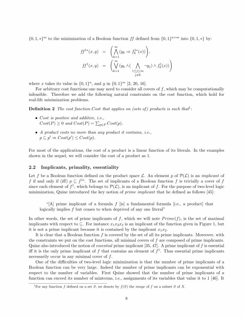
2.2 Implicants, primality, essentiality

Let f be a Boolean function defined on the product space L. An element p of P(L) is an implicant off if and only if (iff) p ⊆ f1∗. The set of implicants of a Boolean function f is trivially a cover of fsince each element of f1, which belongs to P(L), is an implicant of f . For the purpose of two-level logicminimization, Quine introduced the key notion of prime implicant that he defined as follows [45]:

“[A] prime implicant of a formula f [is] a fundamental formula [i.e., a product] thatlogically implies f but ceases to when deprived of any one literal”

In other words, the set of prime implicants of f , which we will note Prime(f), is the set of maximalimplicants with respect to ⊆. For instance x1x2x3 is an implicant of the function given in Figure 1, butit is not a prime implicant because it is contained by the implicant x1x2.

It is clear that a Boolean function f is covered by the set of all its prime implicants. Moreover, withthe constraints we put on the cost functions, all minimal covers of f are composed of prime implicants.Quine also introduced the notion of essential prime implicant [35, 47]. A prime implicant of f is essentialiff it is the only prime implicant of f that contains an element of f1. Thus essential prime implicantsnecessarily occur in any minimal cover of f .

One of the difficulties of two-level logic minimization is that the number of prime implicants of aBoolean function can be very large. Indeed the number of prime implicants can be exponential withrespect to the number of variables. First Quine showed that the number of prime implicants of afunction can exceed its number of minterms, i.e., assignments of its variables that value it to 1 [46]. It

1For any function f defined on a set S, we denote by f(S) the image of f on a subset S of X.

8

ab

cd 00 01 11 10

00

01

11

10

Figure 2: Karnaugh map.

is shown in [13] that the number of prime implicants of functions of n variables is at most O(3n/√n)

and can be at least Ω(3n/n). In [37] is even shown a function that has a minimal sum-of-products madeof n products, but that has 2n − 1 prime implicants.

A cover P of a Boolean function f is irredundant iff there does not exist any proper subset of P thatcovers f . A prime and irredundant cover P of f is locally minimal in the sense that if one eliminates aliteral or a product from P one does no longer have a cover of f . Any minimal prime cover is necessarilyprime and irredundant, but the converse is of course false. Irredundant prime covers are nonethelessinteresting because it can be much less costly to compute such a locally minimal cover than an absoluteminimal one. Most of the techniques developed for exact two-level logic minimization can be modified sothat they produces irredundant prime cover with a lower computational cost. Very different irredundantprime cover computation procedures can be found in [6, 7, 17, 43, 57].

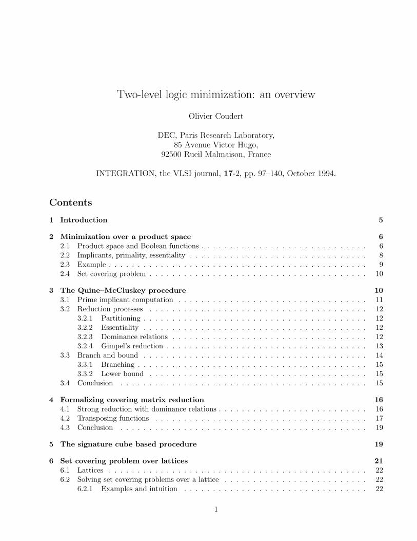
2.3 Example

We illustrate the notions that have been introduced with Karnaugh maps [29]. A Karnaugh map is amatrix that provides a planar representation of elements of the product space B so that products appearas rectangles of the matrix. Each element of the matrix corresponds to an element of B. Variables arepartitioned in two ordered sets, one for the rows of the matrix, and the other for its columns. The rowsand columns are labeled by the values of the corresponding variables so that two consecutive rows orcolumns differ in only one variable value. With this representation, a product of B is a rectangle whosewidth and height are powers of 2.

Figure 2 shows the Karnaugh map of a function f that evalues to 1 for the squares with a blackdot. An implicant of f is a rectangle whose width and height are powers of 2, and that only coversblack dots. An implicant is prime if it is not contained by another implicant. Here there are 5 primeimplicants, i.e., from top to bottom and from left to right: bd, bc, ab, ad, and bcd. All of these primes areessential except ab that covers dots already covered by other primes. Thus the minimal sum-of-productsrepresentation of this function is bd+bc+ad+bcd. Clearly such graphical methods are of limited utilityin solving more complex two-level logic minimization problems.

Figure 3 shows the Karnaugh map of the function presented in the introduction, with some differentcovers. The first one is the irredundant prime cover with 5 prime implicants, the two other ones are thetwo minimal covers made of 4 prime implicants.

9

ab

cd 00 01 11 10

00

01

11

10

ab

cd 00 01 11 10

00

01

11

10

ab

cd 00 01 11 10

00

01

11

10

Figure 3: Karnaugh maps of an irredundant and two minimal prime covers.

2.4 Set covering problem

Sum-of-products minimization is simply a set covering problem. This section introduces notation rele-vant to set covering problems.

We say that a subset R of X × Y is a relation defined on set X × Y . We will write x R y when(x, y) ∈R.

Definition 3 Let X and Y be two sets, R be a relation defined on X×Y , and Cost a cost function thatapplies on subsets of Y . The set covering problem 〈X,Y,R〉 consists of finding a minimal cost subset Sof Y such that for any x of X, there exists an element y of S with x R y.

In the context of set covering, we say that y covers x when x R y. We will note Sol(C) the setof all minimal solutions of a set covering problem C. We say that a set covering problem C2 is weaklyequivalent to a set covering problem C1 if any solution of C2 can be used to build some minimal solutionsof C1. We say that C1 and C2 are strongly equivalent if there is a way of computing Sol(C1) with Sol(C2)and vice versa.

It is convenient to illustrate a set covering problem using a matrix, called its covering matrix. Thematrix associated with the set covering problem 〈X,Y,R〉 has rows labeled with elements of X andcolumns labeled with elements of Y , such that the element [x, y] of the matrix is equal to 1 iff x R y.The set covering problem 〈X,Y,R〉 consists in finding a minimal cost subset of columns that cover allthe rows.

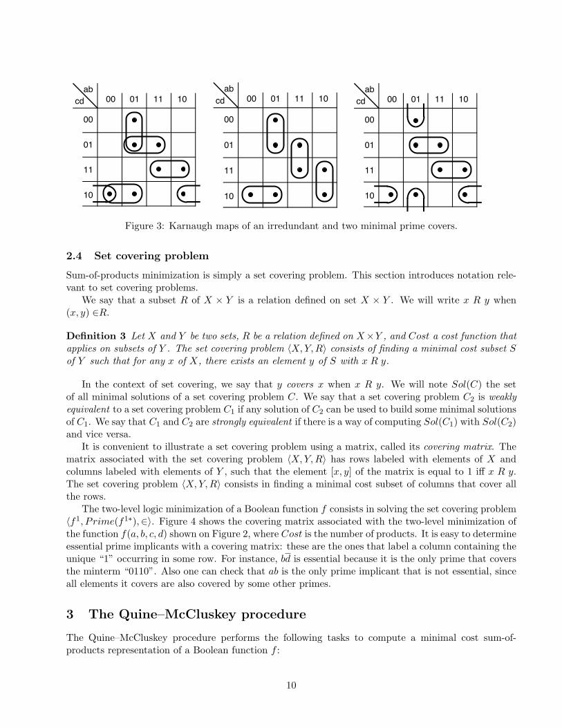
The two-level logic minimization of a Boolean function f consists in solving the set covering problem〈f1, P rime(f1∗),∈〉. Figure 4 shows the covering matrix associated with the two-level minimization ofthe function f(a, b, c, d) shown on Figure 2, where Cost is the number of products. It is easy to determineessential prime implicants with a covering matrix: these are the ones that label a column containing theunique “1” occurring in some row. For instance, bd is essential because it is the only prime that coversthe minterm “0110”. Also one can check that ab is the only prime implicant that is not essential, sinceall elements it covers are also covered by some other primes.

3 The Quine–McCluskey procedure

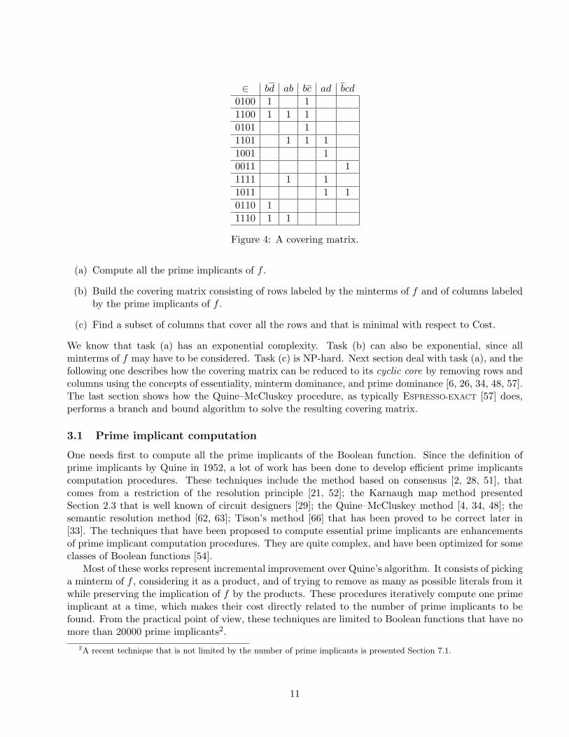
The Quine–McCluskey procedure performs the following tasks to compute a minimal cost sum-of-products representation of a Boolean function f :

10

∈ bd ab bc ad bcd

0100 1 1

1100 1 1 1

0101 1

1101 1 1 1

1001 1

0011 1

1111 1 1

1011 1 1

0110 1

1110 1 1

Figure 4: A covering matrix.

(a) Compute all the prime implicants of f .

(b) Build the covering matrix consisting of rows labeled by the minterms of f and of columns labeledby the prime implicants of f .

(c) Find a subset of columns that cover all the rows and that is minimal with respect to Cost.

We know that task (a) has an exponential complexity. Task (b) can also be exponential, since allminterms of f may have to be considered. Task (c) is NP-hard. Next section deal with task (a), and thefollowing one describes how the covering matrix can be reduced to its cyclic core by removing rows andcolumns using the concepts of essentiality, minterm dominance, and prime dominance [6, 26, 34, 48, 57].The last section shows how the Quine–McCluskey procedure, as typically ESPRESSO-EXACT [57] does,performs a branch and bound algorithm to solve the resulting covering matrix.

3.1 Prime implicant computation

One needs first to compute all the prime implicants of the Boolean function. Since the definition ofprime implicants by Quine in 1952, a lot of work has been done to develop efficient prime implicantscomputation procedures. These techniques include the method based on consensus [2, 28, 51], thatcomes from a restriction of the resolution principle [21, 52]; the Karnaugh map method presentedSection 2.3 that is well known of circuit designers [29]; the Quine–McCluskey method [4, 34, 48]; thesemantic resolution method [62, 63]; Tison’s method [66] that has been proved to be correct later in[33]. The techniques that have been proposed to compute essential prime implicants are enhancementsof prime implicant computation procedures. They are quite complex, and have been optimized for someclasses of Boolean functions [54].

Most of these works represent incremental improvement over Quine’s algorithm. It consists of pickinga minterm of f , considering it as a product, and of trying to remove as many as possible literals from itwhile preserving the implication of f by the products. These procedures iteratively compute one primeimplicant at a time, which makes their cost directly related to the number of prime implicants to befound. From the practical point of view, these techniques are limited to Boolean functions that have nomore than 20000 prime implicants2.

2A recent technique that is not limited by the number of prime implicants is presented Section 7.1.

11

R y1 y2 y3 y4 y5x1 1 1 1 1

x2 1 1 1 1

x3 1 1

x4 1 1 1

x5 1 1

x6 1

→

R y1 y2 y3 y4x1 1 1 1 1

x2 1 1 1 1

x3 1 1

x5 1 1

Figure 5: Reduction by essentiality.

3.2 Reduction processes

Once the covering matrix has been built, it can be split into several independent minimizing problems,and it can be reduced by iteratively removing its rows and columns. We recall here the main techniquesthat can be used to reduce the size of the optimization problem [24, 44, 57].

3.2.1 Partitioning

If the rows and the columns of a covering matrix can be permuted to yield a covering matrix that ispartitioned in diagonal blocks Bk as follows, where 1’s occur only in these blocks, then any minimalsolution of the original problem is the union of minimal solutions of the blocks Bk. The partionning ofa set covering matrix is easily obtained by noting that two rows that cover a common column are inthe same block.

B1

B2

. . .

Bn

3.2.2 Essentiality

Let 〈X,Y,R〉 be a set covering problem. An element y of Y is essential iff it is the only one that coversan element x of X. When Y is a set of prime implicants, this notion is the same as essential primeimplicants. Since essential elements belong necessarily to any minimal solution, we can remove from thecovering matrix all columns labeled by essential elements as well as the rows they cover. This reductionyields a strongly equivalent set covering problem, since all minimal solutions of the original problemcan be obtained by adding all essential elements to all minimal solutions of the reduced problem [47].

For instance consider the left-hand side covering matrix of Figure 5. The only element that coversx6 is y5. Thus y5 is necessary in all minimal solutions of this set covering problem. Thus the columnlabeled by y5 can be removed from the matrix, as well as all rows covered by y5, i.e., x4 and x6. Thisgenerates the strongly equivalent set covering problem whose matrix is shown on the right-hand side ofFigure 5.

3.2.3 Dominance relations

Dominance relations have been introduced to reduce the size of a set covering problem by removingrows and columns from its matrix and yielding a new covering matrix that is (weakly) equivalent to theoriginal one. We give here an intuitive idea of dominance relations, and the way they are used in the

12

R y1 y2 y3 y4 y5x1 1 1 1 1

x2 1 1 1 1

x3 1 1

x4 1 1 1

x5 1 1

x6 1

→R y1 y2 y3 y4 y5x3 1 1

x6 1

Figure 6: Reduction by domination on X.

R y1 y2 y3 y4 y5x1 1 1 1 1

x2 1 1 1 1

x3 1 1

x4 1 1 1

x5 1 1

x6 1

→

R y1 y5x1 1

x2 1

x3 1

x4 1 1

x5 1

x6 1

Figure 7: Reduction by domination on Y .

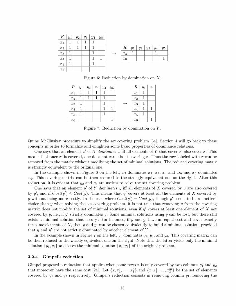
Quine–McCluskey procedure to simplify the set covering problem [34]. Section 4 will go back to theseconcepts in order to formalize and enlighten some basic properties of dominance relations.

One says that an element x′ of X dominates x iff all elements of Y that cover x′ also cover x. Thismeans that once x′ is covered, one does not care about covering x. Thus the row labeled with x can beremoved from the matrix without modifying the set of minimal solutions. The reduced covering matrixis strongly equivalent to the original one.

In the example shown in Figure 6 on the left, x3 dominates x1, x2, x4 and x5, and x6 dominatesx4. This covering matrix can be then reduced to the strongly equivalent one on the right. After thisreduction, it is evident that y2 and y3 are useless to solve the set covering problem.

One says that an element y′ of Y dominates y iff all elements of X covered by y are also coveredby y′, and if Cost(y′) ≤ Cost(y). This means that y′ covers at least all the elements of X covered byy without being more costly. In the case where Cost(y′) = Cost(y), though y′ seems to be a “better”choice than y when solving the set covering problem, it is not true that removing y from the coveringmatrix does not modify the set of minimal solutions, even if y′ covers at least one element of X notcovered by y, i.e., if y′ strictly dominates y. Some minimal solutions using y can be lost, but there stillexists a minimal solution that uses y′. For instance, if y and y′ have an equal cost and cover exactlythe same elements of X, then y and y′ can be chosen equivalently to build a minimal solution, providedthat y and y′ are not strictly dominated by another element of Y .

In the example shown in Figure 7 on the left, y1 dominates y2, y3, and y4. This covering matrix canbe then reduced to the weakly equivalent one on the right. Note that the latter yields only the minimalsolution y1, y5 and loses the minimal solution y4, y5 of the original problem.

3.2.4 Gimpel’s reduction

Gimpel proposed a reduction that applies when some rows x is only covered by two columns y1 and y2that moreover have the same cost [24]. Let x, x11, . . . , xn1 and x, x12, . . . , xm2 be the set of elementscovered by y1 and y2 respectively. Gimpel’s reduction consists in removing column y1, removing the

13

R y1 y2 y3 y4 y5x 1 1

x11 1 1

x21 1 1

x12 1 1 1

x22 1 1

x6 1 1

→

R y2 y3 y4 y5x1,1 1 1 1

x1,2 1 1 1

x2,1 1 1 1

x2,2 1 1 1

x6 1 1

Figure 8: Gimpel’s reduction on x.

n +m + 1 rows covered by y1 and y2, and adding nm new rows xi,j (1 ≤ i ≤ n and 1 ≤ j ≤ m) suchthat the row xi,j is covered by the set of columns

y ∈ Y | xi1 R y ∨ xj2 R y − y1.

Let S be a minimal solution of this new problem. Then a minimal solution of the original set coveringproblem is derived as follows [53]. If S is such that S ∩ y ∈ Y | xi1 R y 6= Ø for 1 ≤ i ≤ n, then addy2 to S. Otherwise add y1 to S.

Consider the example shown in Figure reffig:gimpel. The row x is only covered by two columns thathave the same cost, namely y1 and y2. All rows covered by y1 and y2 are removed, namely rows x up tox22, and colums y1 is removed from the matrix. Here we have n = m = 2, so we add nm = 4 new rows asdescribed above. For instance rows x2,1 is covered by columns that cover either x21 or x12 beside y1, i.e.,y2, y3, y5. Gimpel’s reduction produces the covering matrix shown on the right-hand side of Figure 8.One of its minimal solution is S = y3, y5, which intersects both the sets y ∈ Y | xi1 R y for 1 ≤ i ≤ 2,i.e., y1, y5 and y1, y3, thus adding y2 to S produces y2, y3, y5 which is a minimal solution of theoriginal problem. Another minimal solution of the right-hand side problem is S = y2, y5. The set Sdoes not intersects the set y1, y3, and adding y1 to S produces y1, y2, y5 which is still a minimalsolution of the original problem.

Gimpel’s reduction yields a new set covering problem with one less column but with nm−n−m−1more rows. Adding new rows can produce new dominations between rows and columns, which canreduce the covering matrix. However, from the practical point of view, it is better to allow Gimpel’sreduction when it guarantees to produce a smaller covering matrix, i.e., when nm− n−m− 1 ≤ 0.

3.3 Branch and bound

When the reduction processes described above (essentiality, and dominance relations on X and Y )are iteratively applied, one eventually produced a covering matrix that the reduction processes do notmodify anymore. This fixpoint is called the cyclic core of 〈X,Y,R〉. If this cyclic core is empty, theset of all essential elements that have been found during the reduction process constitutes a minimalsolution of the original problem.

If the cyclic core is not empty, the minimization can be terminated using a branch-and-boundalgorithm. One chooses an element of y, and generates two subproblems, one resulting from choosingy in the minimal solution, the other resulting from discarding y from Y . These two subproblems areconsequently simplified, i.e., their cyclic cores are computed, and then recursively solved. The minimalsolution of the original problem is the minimum of both of the minimal solutions of the two subproblems.

14

3.3.1 Branching

Heuristics to properly choose an element of Y as belonging to the minimal solution are discussedin [6, 34, 57]. A natural heuristics consists in choosing an element y that cover the largest number ofelements of X. However experimental results show that it is not the best heuristics. A much betterheuristics proposed in [57] consists in, given a cyclic core 〈X,Y,R〉, choosing an element y that maximizesChoose(y):

Choose(y) =∑

xRy

1

|y ∈ Y | x R y| − 1

This cost function increases with the number of elements that y cover, but also with the “quality” ofthe elements it covers. The less an element x is covered, the harder it is to cover it, the larger will beits contribution to the cost function. Thus this cost function favors elements y that cover difficult x’s.

3.3.2 Lower bound

If we know a lower bound of the minimal solution of a subproblem yielded at some point of the branchingalgorithm, one can prune the recursion as soon as the lower bound is greater or equal to the best solutionfound so far. It is critical to provide an accurate lower bound to terminate useless searches as early aspossible.

Let 〈X,Y,R〉 be a set covering problem, and let X ′ be a subset of X such that for any two differentelements x1 and x2 of X ′, all elements y that cover x1 do not cover x2 and conversely. The set X ′,which we will call an independent subset of X, provides us with the lower bound

∑

x∈X′

miny

xRy

Cost(y),

since this is the minimum cost necessary to cover the elements of X ′. Though finding an independentsubset that maximizes this lower bound is an NP-complete problem, heuristics in practice yields a quitegood lower bound, except for examples that have a large number of y’s compared to the number of x’s(for instance the big random examples of the MCNC benchmark [68]).

3.4 Conclusion

The two-level logic minimization of a Boolean function f consists in solving the set covering problem〈f1, P rime(f1∗),∈〉. The Quine–McCluskey procedure, e.g., ESPRESSO-EXACT, computes the cyclic coreof this covering matrix using row/column removal based on dominance and essentiality. If the cycliccore is empty, the minimization is done, else a row is selected and the procedure is iterated. A branch-and-bound algorithm can then provide a minimal solution [6, 34, 57].

In the Quine–McCluskey procedure, the elements of f to be covered (i.e., the set X) and the primeimplicants of f (i.e., the set Y ) are explicitly represented. This implies that the cost of this procedureis directly related to the number of prime implicants, and it cannot be applied on functions that havelarge numbers of prime implicants.

To overcome this limitation, Swamy, McGeer, and Brayton have introduced in [65] an implicit cycliccore computation procedure, in which the covering matrix is implicitly represented with a couple ofBDDs (Binary Decision Diagrams are a canonical representation of Boolean functions, see appendix A).The set of rows, i.e., the minterms to be covered, is represented with a BDD, and the set of columnsis represented with the BDD of the characteristic function of the prime implicants that can be used

15

to cover the minterms. Initially, the covering matrix is represented by the BDD of the function f tominimize, and by the BDD of all the prime implicants of f . The idea is to compute, at each step ofthe cyclic core computation, two BDDs representing the minterm dominance relation and the primedominance relation respectively, and then to extract from these two BDDs a new implicit coveringmatrix. The problem with this procedure is that the BDDs of the dominance relations are computedby evaluating complex quantified Boolean formulas, which makes the procedure difficult to apply onlarge examples [65]. It has been shown later that the use of recursive operators for the building ofthe minterm and prime dominance relations make the implicit cyclic computation much more efficient.However, it happens that the computation fails for some examples because the BDDs of the dominancerelations are too big to allow extraction of the reduced covering matrix.

4 Formalizing covering matrix reduction

This section formalizes the reduction processes presented above, and shows that some new concepts canbe figured out to reduce and solve a set covering problem [19] 〈X,Y,R〉 with respect to any additivecost function Cost.

4.1 Strong reduction with dominance relations

We first clarify the underlying structure of the dominance relations, and show how to reduce a coveringmatrix to a strongly equivalent problem.

A quasi order is a reflexive and transitive relation, and will be noted ≺. A partial order is areflexive, transitive, and antisymmetric relation, and will be noted or ⊑. An equivalence relation isa reflexive, transitive, and symmetric relation, and will be noted ≡. Let ≡ be an equivalence relationon Z. The quotient set, noted Z/ ≡, is the partition of Z made of the equivalence classes of ≡.Given a set Z quasi ordered by ≺, we denote by max≺ Z its set of maximal elements, i.e., the setz ∈ Z | ∀z′ ∈ Z, z ≺ z′ ⇒ z = z′.

Let 〈X,Y,R〉 be a set covering problem, and Cost any additive cost function. The dominancerelations that we will note ≺Y and ≺X in the following, are defined on X and Y respectively as follows:

x ≺Y x′ ⇔ y ∈ Y | x′ R y ⊆ y ∈ Y | x R y,y ≺X y′ ⇔ x ∈ X | x R y ⊆ x ∈ X | x R y′ ∧ Cost(y′) ≤ Cost(y).

Since ⊆ and ≤ are reflexive and transitive, the dominance relations ≺Y and ≺X are quasi orders on Xand Y respectively. We now introduce the following notation.

Definition 4 Let ≺ be a quasi order on a set Z. We associate with ≺ the equivalence relation ≡ definedby (z ≡ z′) ⇔ ((z ≺ z′) ∧ (z′ ≺ z)). The projection of the quasi order ≺ on Z/≡ is a partial order,which we denote with . We denote by π the function that maps each element of Z onto its equivalenceclass, and by ρ a function that map each equivalence class onto one of its element.

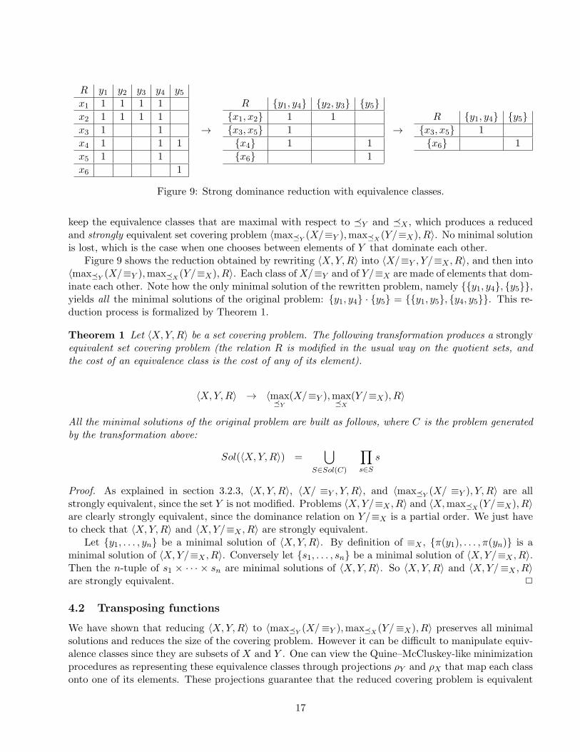
The process of row and column removing described in Section 3.2 generates a weakly equivalent setcovering problem, because an arbitrary choice is made between two columns that dominate each other.A stronger reduction process consists in considering two elements that dominate each other as belongingto the same class. Indeed, this consists in partitioning X (respectively Y ) into the equivalence classesX/≡Y (respectively Y/≡X) induced by the dominance relation ≺Y (respectively ≺X). Then we only

16

R y1 y2 y3 y4 y5x1 1 1 1 1

x2 1 1 1 1

x3 1 1

x4 1 1 1

x5 1 1

x6 1

→

R y1, y4 y2, y3 y5x1, x2 1 1

x3, x5 1

x4 1 1

x6 1

→R y1, y4 y5

x3, x5 1

x6 1

Figure 9: Strong dominance reduction with equivalence classes.

keep the equivalence classes that are maximal with respect to Y and X , which produces a reducedand strongly equivalent set covering problem 〈maxY

(X/≡Y ),maxX(Y/≡X), R〉. No minimal solution

is lost, which is the case when one chooses between elements of Y that dominate each other.Figure 9 shows the reduction obtained by rewriting 〈X,Y,R〉 into 〈X/≡Y , Y/≡X , R〉, and then into

〈maxY(X/≡Y ),maxX

(Y/≡X), R〉. Each class ofX/≡Y and of Y/≡X are made of elements that dom-inate each other. Note how the only minimal solution of the rewritten problem, namely y1, y4, y5,yields all the minimal solutions of the original problem: y1, y4 · y5 = y1, y5, y4, y5. This re-duction process is formalized by Theorem 1.

Theorem 1 Let 〈X,Y,R〉 be a set covering problem. The following transformation produces a stronglyequivalent set covering problem (the relation R is modified in the usual way on the quotient sets, andthe cost of an equivalence class is the cost of any of its element).

〈X,Y,R〉 → 〈maxY

(X/≡Y ),maxX

(Y/≡X), R〉

All the minimal solutions of the original problem are built as follows, where C is the problem generatedby the transformation above:

Sol(〈X,Y,R〉) =⋃

S∈Sol(C)

∏

s∈S

s

Proof. As explained in section 3.2.3, 〈X,Y,R〉, 〈X/ ≡Y , Y, R〉, and 〈maxY(X/ ≡Y ), Y, R〉 are all

strongly equivalent, since the set Y is not modified. Problems 〈X,Y/≡X , R〉 and 〈X,maxX(Y/≡X), R〉

are clearly strongly equivalent, since the dominance relation on Y/≡X is a partial order. We just haveto check that 〈X,Y,R〉 and 〈X,Y/≡X , R〉 are strongly equivalent.

Let y1, . . . , yn be a minimal solution of 〈X,Y,R〉. By definition of ≡X , π(y1), . . . , π(yn) is aminimal solution of 〈X,Y/≡X , R〉. Conversely let s1, . . . , sn be a minimal solution of 〈X,Y/≡X , R〉.Then the n-tuple of s1 × · · · × sn are minimal solutions of 〈X,Y,R〉. So 〈X,Y,R〉 and 〈X,Y/≡X , R〉are strongly equivalent. 2

4.2 Transposing functions

We have shown that reducing 〈X,Y,R〉 to 〈maxY(X/≡Y ),maxX

(Y/≡X), R〉 preserves all minimalsolutions and reduces the size of the covering problem. However it can be difficult to manipulate equiv-alence classes since they are subsets of X and Y . One can view the Quine–McCluskey-like minimizationprocedures as representing these equivalence classes through projections ρY and ρX that map each classonto one of its elements. These projections guarantee that the reduced covering problem is equivalent

17

to the original one, but it is only weakly equivalent if one cannot evaluate ρ−1X , i.e., πX . This section

shows that, instead of using such projections, one can use an isomorphism that maps the classes thatmust be manipulated onto objects whose manipulation is less costly [19].

Definition 5 Let (Z,≺) be a quasi ordered set. A transposing function τ is a morphism3 that maps(Z,≺) onto a partially ordered set (τ(Z),⊑), such that τ(z) ⊑ τ(z′) iff z ≺ z′.

Any quasi ordered set (Z,≺) has at least one transposing function. For instance, the function τ(z) =z′ ∈ Z | z′ ≺ z is a transposing function that maps (Z,≺) into the partially ordered set (2Z ,⊆). Wecall this particular morphism the universal transposing function of (Z,≺).

If τ is a transposing function from the quasi ordered set (Z,≺) into (τ(Z),⊑), then the latter isisomorphic to (Z/≡,) through τ ρ. We thus obtain the following commutative diagram:

(Z/≡,) −→ max(Z/≡)

(Z,≺)րπ

ցτ

x

y

τρ

x

y

τρ

(τ(Z),⊑) −→ max⊑ τ(Z)

Note that the range of τ can be any set, as soon as it is partially ordered. Thus the transformationthat τ performs is useful because it can be much more efficient to represent and manipulate elementsof τ(Z) than elements of 2Z .

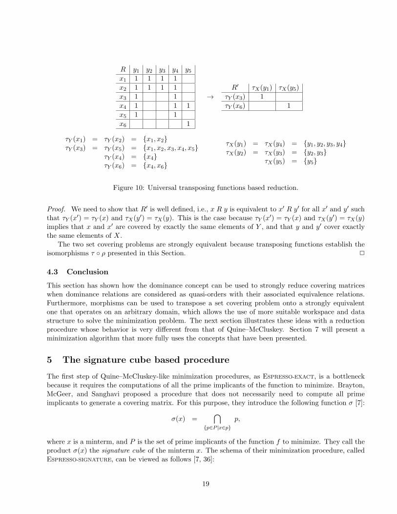
Using transposing functions to reduce set covering problems is then straightforward. Figure 10 il-lustrates how transposing functions reduce a covering matrix 〈X,Y,R〉. Let τY and τX be the universaltransposing functions of the dominance relations ≺Y and ≺X respectively. Then maxY

(X/≡Y ) (re-spectively maxX

(Y/≡X)) is isomorphic to max⊆ τY (X) (respectively max⊆ τX(Y )). Thus the reducedand strongly equivalent set covering problem 〈maxY

(X/≡Y ),maxX(Y/≡X), R〉 introduced in pre-

vious section is isomorphic to 〈max⊑YτY (X),max⊑X

τX(Y ), R′〉, where R′ is the relation induced byR through τY and τX . From the covering matrix given on the left, we compute the sets τY (xk) andτX(yk), and produce the reduced and strongly equivalent covering matrix on the right by keeping setsthat are maximal w.r.t. ⊆. The only minimal solution of this covering matrix is τX(y1), τX(y5). Sothe minimal solutions of the original problem is given by τ−1

X (τX(y1)) · τ−1X (τX(y5)) = y1, y4 · y5 =

y1, y5, y4, y5. Theorem 2 formalizes this new transformation.

Theorem 2 Let 〈X,Y,R〉 be a set covering problem, τY be a transposing function from (X,≺Y ) into(τY (X),⊑Y ), and τX be a transposing function from (Y,≺X) into (τX(Y ),⊑X). The following trans-formation, where R′ is defined by τY (x) R

′ τX(y) ⇔ x R y, produces a strongly equivalent set coveringproblem.

〈X,Y,R〉 → 〈max⊑Y

τY (X),max⊑X

τX(Y ), R′〉.

All the minimal solutions of the original problem are built as follows, where C is the problem generatedby the transformation above:

Sol(〈X,Y,R〉) =⋃

S∈Sol(C)

∏

s∈S

τ−1X (s).

3Most of the time it is not injective.

18

R y1 y2 y3 y4 y5x1 1 1 1 1

x2 1 1 1 1

x3 1 1

x4 1 1 1

x5 1 1

x6 1

→R′ τX(y1) τX(y5)

τY (x3) 1

τY (x6) 1

τY (x1) = τY (x2) = x1, x2τY (x3) = τY (x5) = x1, x2, x3, x4, x5

τY (x4) = x4τY (x6) = x4, x6

τX(y1) = τX(y4) = y1, y2, y3, y4τX(y2) = τX(y3) = y2, y3

τX(y5) = y5

Figure 10: Universal transposing functions based reduction.

Proof. We need to show that R′ is well defined, i.e., x R y is equivalent to x′ R y′ for all x′ and y′ suchthat τY (x

′) = τY (x) and τX(y′) = τX(y). This is the case because τY (x′) = τY (x) and τX(y′) = τX(y)

implies that x and x′ are covered by exactly the same elements of Y , and that y and y′ cover exactlythe same elements of X.

The two set covering problems are strongly equivalent because transposing functions establish theisomorphisms τ ρ presented in this Section. 2

4.3 Conclusion

This section has shown how the dominance concept can be used to strongly reduce covering matriceswhen dominance relations are considered as quasi-orders with their associated equivalence relations.Furthermore, morphisms can be used to transpose a set covering problem onto a strongly equivalentone that operates on an arbitrary domain, which allows the use of more suitable workspace and datastructure to solve the minimization problem. The next section illustrates these ideas with a reductionprocedure whose behavior is very different from that of Quine–McCluskey. Section 7 will present aminimization algorithm that more fully uses the concepts that have been presented.

5 The signature cube based procedure

The first step of Quine–McCluskey-like minimization procedures, as ESPRESSO-EXACT, is a bottleneckbecause it requires the computations of all the prime implicants of the function to minimize. Brayton,McGeer, and Sanghavi proposed a procedure that does not necessarily need to compute all primeimplicants to generate a covering matrix. For this purpose, they introduce the following function σ [7]:

σ(x) =⋂

p∈P |x∈p

p,

where x is a minterm, and P is the set of prime implicants of the function f to minimize. They call theproduct σ(x) the signature cube of the minterm x. The schema of their minimization procedure, calledESPRESSO-SIGNATURE, can be viewed as follows [7, 36]:

19

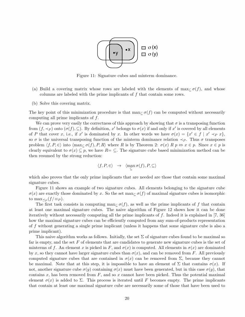
xy (y)σ

(x)σ

Figure 11: Signature cubes and minterm dominance.

(a) Build a covering matrix whose rows are labeled with the elements of max⊆ σ(f), and whosecolumns are labeled with the prime implicants of f that contain some rows.

(b) Solve this covering matrix.

The key point of this minimization procedure is that max⊆ σ(f) can be computed without necessarilycomputing all prime implicants of f .

We can prove very easily the correctness of this approach by showing that σ is a transposing functionfrom (f,≺P ) onto (σ(f),⊆). By definition, x′ belongs to σ(x) if and only if x′ is covered by all elementsof P that cover x, i.e., if x′ is dominated by x. In other words we have σ(x) = x′ ∈ f | x′ ≺P x,so σ is the universal transposing function of the minterm dominance relation ≺P . Thus σ transposesproblem 〈f, P,∈〉 into 〈max⊆ σ(f), P,R〉 where R is by Theorem 2: σ(x) R p ⇔ x ∈ p. Since x ∈ p isclearly equivalent to σ(x) ⊆ p, we have R= ⊆. The signature cube based minimization method can bethen resumed by the strong reduction:

〈f, P,∈〉 → 〈max⊆

σ(f), P,⊆〉

which also proves that the only prime implicants that are needed are those that contain some maximalsignature cubes.

Figure 11 shows an example of two signature cubes. All elements belonging to the signature cubeσ(x) are exactly those dominated by x. So the set max⊆ σ(f) of maximal signature cubes is isomorphicto maxP

(f/≡P ).The first task consists in computing max⊆ σ(f), as well as the prime implicants of f that contain

at least one maximal signature cubes. The naive algorithm of Figure 12 shows how it can be doneiteratively without necessarily computing all the prime implicants of f . Indeed it is explained in [7, 36]how the maximal signature cubes can be efficiently computed from any sum-of-products representationof f without generating a single prime implicant (unless it happens that some signature cube is also aprime implicant).

This naive algorithm works as follows. Initially, the set Σ of signature cubes found to be maximal sofar is empty, and the set F of elements that are candidates to generate new signature cubes is the set ofminterms of f . An element x is picked in F , and σ(x) is computed. All elements in σ(x) are dominatedby x, so they cannot have larger signature cubes than σ(x), and can be removed from F . All previouslycomputed signature cubes that are contained in σ(x) can be removed from Σ, because they cannotbe maximal. Note that at this step, it is impossible to have an element of Σ that contains σ(x). Ifnot, another signature cube σ(y) containing σ(x) must have been generated, but in this case σ(y), thatcontains x, has been removed from F , and so x cannot have been picked. Thus the potential maximalelement σ(x) is added to Σ. This process is iterated until F becomes empty. The prime implicantsthat contain at least one maximal signature cube are necessarily some of those that have been used to

20

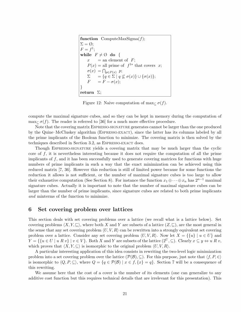
function ComputeMaxSigma(f);Σ = Ø;F = f1;while F 6= Ø do

x = an element of F ;P (x) = all prime of f1∗ that covers x;σ(x) =

⋂

p∈P (x) p;

Σ = q ∈ Σ | q 6⊆ σ(x) ∪ σ(x);F = F − σ(x);

return Σ;

Figure 12: Naive computation of max⊆ σ(f).

compute the maximal signature cubes, and so they can be kept in memory during the computation ofmax⊆ σ(f). The reader is referred to [36] for a much more effective procedure.

Note that the covering matrix ESPRESSO-SIGNATURE generates cannot be larger than the one producedby the Quine–McCluskey algorithm (ESPRESSO-EXACT), since the latter has its columns labeled by allthe prime implicants of the Boolean function to minimize. The covering matrix is then solved by thetechniques described in Section 3.2, as ESPRESSO-EXACT does.

Though ESPRESSO-SIGNATURE yields a covering matrix that may be much larger than the cycliccore of f , it is nevertheless interesting because it does not require the computation of all the primeimplicants of f , and it has been successfully used to generate covering matrices for functions with hugenumbers of prime implicants in such a way that the exact minimization can be achieved using thisreduced matrix [7, 36]. However this reduction is still of limited power because for some functions thereduction it allows is not sufficient, or the number of maximal signature cubes is too large to allowtheir exhaustive computation (See Section 8). For instance the function x1⊕· · ·⊕xn has 2n−1 maximalsignature cubes. Actually it is important to note that the number of maximal signature cubes can belarger than the number of prime implicants, since signature cubes are related to both prime implicantsand minterms of the function to minimize.

6 Set covering problem over lattices

This section deals with set covering problems over a lattice (we recall what is a lattice below). Setcovering problems 〈X,Y,⊑〉, where both X and Y are subsets of a lattice (Z,⊑), are the most general inthe sense that any set covering problem 〈U, V,R〉 can be rewritten into a strongly equivalent set coveringproblem over a lattice. Consider any set covering problem 〈U, V,R〉. Now let X = u | u ∈ U andY = u ∈ U | u R v | v ∈ V . BothX and Y are subsets of the lattice (2U ,⊆). Clearly x ⊆ y ⇔ u R v,which proves that 〈X,Y,⊆〉 is isomorphic to the original problem 〈U, V,R〉.

A particular interesting application of this idea consists in rewriting the two-level logic minimizationproblem into a set covering problem over the lattice (P(B),⊆). For this purpose, just note that 〈f, P,∈〉is isomorphic to 〈Q,P,⊆〉, where Q = q ∈ P(B) | x ∈ f, x = q. Section 7 will be a consequence ofthis rewriting.

We assume here that the cost of a cover is the number of its elements (one can generalize to anyadditive cost function but this requires technical details that are irrelevant for this presentation). This

21

section introduces an essential result for solving set covering problems over a lattice.

6.1 Lattices

A complete lattice (Z,⊑) is a partially ordered set such that any non empty subset of Z has a greatestlower bound and a least upper bound with respect to ⊑. If X is a subset of Z, we denote sup⊑X theleast upper bound of X w.r.t ⊑, i.e., the unique minimal (w.r.t ⊑) element z of Z such that x ⊑ z forall elements x of X. We denote inf⊑X the greatest lower bound of X, i.e., the unique maximal elementz of Z such that z ⊑ x for all elements x of X.

Since the structure (Z,⊒) is also a lattice, the principle of duality implies that, if a statement istrue on (Z,⊑), then the dual statement obtained by interchanging ⊑ and ⊒ can also be deduced. Notethat inf⊑ = sup⊒.

6.2 Solving set covering problems over a lattice

The aim of this section is to prove the following fundamental result.

Theorem 3 Let (Z,⊑) be a complete lattice. Let X and Y be subsets of Z. The fixpoint obtainedby applying the following transformations is strongly equivalent to the cyclic core of the set coveringproblem 〈X,Y,⊑〉.

〈X,Y,⊑〉 1→ 〈X,max⊑

τX,⊑(Y ),⊑〉,

〈X,Y,⊑〉 2→ 〈max⊑

τY,⊒(X), Y,⊑〉,

〈X,Y,⊑〉 3→ 〈X − E, Y − E,⊑〉 with E = X ∩ Y

where τW,⊑ is the function defined from Z into Z by:

τW,⊑(z) = sup⊑

w ∈ W | w ⊑ z.

All the minimal solutions of the original problem are built as follows. Let C be the fixpoint generated bythe transformations above, and F be the union of the sets E yielded by the third rewriting rule duringthe fixpoint computation. Then

Sol(〈X,Y,R〉) =⋃

S∈Sol(C)

∏

z∈S∪F

y ∈ Y | z ⊑ y.

We first present examples to give the intuitive ideas beyond this rewriting system. We then proveTheorem 3 in three steps. We first justify rule (1) and (2) by showing that τW,⊑ is a transposing functionthat can be used to capture dominance on both X and Y . We show that rule (3) consists of computingthe set E of essential elements of Y and applying the corresponding reduction. Finally we prove thatrecovering the minimal solutions of the original problem can be done as described above.

6.2.1 Examples and intuition

Consider the set covering problem over a lattice given on the left-hand side of Figure 13. Each dot isan element of the lattice (Z,⊑). Black dots are the elements of X, and gray boxes are the elements of

22

τ ( ),

Figure 13: Computing τX,⊑(Y ) on a lattice.

τ ( ),

Figure 14: Computing τY,⊒(X) on a lattice.

Y . The maximal element of Z is the top dot of the diagram, and its minimal element is the bottomdot. The partial order ⊑ is denoted by edges between an upper dot and a lower dot.

The rewriting of Y into τX,⊑(Y ) is given by the right-hand side diagram of Figure 13. Each box y ismapped on the least upper bound of the set of black dots it covers. The two right-hand side boxes aremapped on the same element of Z because they cover exactly the same elements of X. Note that someboxes of Y remain invariant, while some others are mapped onto new elements of Z, some of them evenbeing elements of X. The cardinality of τX,⊑(Y ) is strictly less than the cardinality of Y because thetwo left-hand side boxes have been mapped on the same box by τX,⊑, since they cover exactly the sameblack dots. Keeping the maximal boxes with respect to ⊑ produces a set made of three boxes, whichis the only minimal covering of the reduced problem. From this set we can recover the two minimalsolutions of the original problem as it is described by Theorem 3.

Figure 14 gives the rewriting of X into τY,⊒(X) on the same covering problem. Each black dot x ismapped on the greatest lower bound of the set of boxes that cover it. The two right-hand side blackdots are mapped on the same element of Z because they are covered by the same set of boxes. Notethat τY,⊒(x) = inf⊑y ∈ Y | x ⊑ y. Here again, some elements of X remains invariant, while someothers are mapped onto new elements of Z, some of them even being elements of Y . The cardinalityof τY,⊒(X) is strictly less than X’s one because the two left-hand side black dots have been mapped onthe same dot by τY,⊒, since they are covered by the same boxes. There are only four black dots thatare maximal with respect to ⊑. We can then obtain directly the two minimal solution of the originalproblem.

Figure 15 gives on the left-hand side a set covering problem 〈X,Y,⊑〉 over a lattice (Z,⊑) where Yis maximal. Then it shows the set covering problem obtained after having applied τY,⊒, and finally thediagram obtained by extracting from τY,⊒(X) the maximal elements. The elements of sets Y ∩ τY,⊒(X)and Y ∩max⊑ τY,⊒(X) are denoted by a box with a black dot inside. Both of these sets are equal to

23

τ max( ) ( ),

Figure 15: Computing the essential elements.

a set E. Clearly E is the set of essential elements of the original problem. Removing E from the setof boxes consists in removing essential elements from Y , and removing E from the set of black dotsconsists in removing the elements of X that are covered by essential elements. This problem has finallyfour minimal solutions.

6.2.2 The transposing function τW,⊑

We prove the first result that will justify rule (1) and (2).

Lemma 1 Let (Z,⊑) be a complete lattice. Let W be a subset of Z. Let ≺W,⊑ be the quasi-order definedon Z by

z ≺W,⊑ z′ ⇔ w ∈ W | w ⊑ z ⊆ w ∈ W | w ⊑ z′,

and τW,⊑ be the function defined from Z into Z by

τW,⊑(z) = sup⊑

w ∈ W | w ⊑ z.

The function τW,⊑ is a transposing function from (Z,≺W,⊑) into (Z,⊑).

Proof. The proof is based on the two key properties of τW,⊑ that come directly from its definition: (1)for all z of Z we have τW,⊑(z) ⊑ z ; (2) for all w of W and all z of Z, w ⊑ z is equivalent to w ⊑ τW,⊑(z).

Since for any subsets S and S′ of Z, S ⊆ S′ implies that supS ⊑ supS′, we have z ≺W,⊑ z′

implies τW,⊑(z) ⊑ τW,⊑(z′). Conversely, assume that τW,⊑(z) ⊑ τW,⊑(z

′). Then by (1) and (2) we havew ⊑ τW,⊑(z) ⊑ τW,⊑(z

′) ⊑ z′ for all element w of W such that w ⊑ z. This means that we have w ⊑ z′

for all element w of W such that w ⊑ z, i.e., z ≺W,⊑ z′. So we have shown that z ≺W,⊑ z′ is equivalentto τW,⊑(z) ⊑ τW,⊑(z

′). Thus τW,⊑ is a transposing function from (Z,≺W,⊑) into (Z,⊑). 2

Corollary 1 Let (Z,⊑) be a complete lattice. Let 〈X,Y,⊑〉 be a set covering problem, where X and Yare subsets of Z. It is strongly equivalent to 〈max⊑ τY,⊒(X),max⊑ τX,⊑(Y ),⊑〉.

Proof. Lemma 1 proved that τX,⊑ is a transposing function from (Z,≺X,⊑) into (Z,⊑). By dualityand Lemma 1, the function τY,⊒ is a transposing function from (Z,≺Y,⊒) into (Z,⊒), i.e., a trans-posing function from (Z,≻Y,⊒) into (Z,⊑). The dominance relation on Y is ≺X,⊑, and the dom-inance relation on X is ≻Y,⊒. So by Theorem 2, the problem 〈X,Y,⊑〉 is strongly equivalent to〈max⊑ τY,⊒(X),max⊑ τX,⊑(Y ), R〉, where R is defined by x ⊑ y ⇔ τY,⊒(x) R y. By (2) and dual-ity, y ⊒ x is equivalent to y ⊒ τY,⊒(x) for all y of Y , so we have R=⊑. 2

24

We have justified the first and second reduction, namely the set covering problem 〈X,Y,⊑〉 is stronglyequivalent to 〈X,max⊑ τX,⊑(Y ),⊑〉 and 〈max⊑ τY,⊒(X), Y,⊑〉. The advantage of the transposing func-tions τX,⊑ and τY,⊒ is that they map Z into Z, which preserves the nature of the set covering problem:they produce strongly equivalent problems that have still the form 〈X,Y,⊑〉, where both X and Y aresubsets of the lattice (Z,⊑).

6.2.3 Essential elements

We now prove the second result. This nice property is a consequence of the definition of τY,⊒, which isa transposing function that acts as a filter on the lattice and maps (Z,⊑) into itself.

Lemma 2 Let (Z,⊑) be a complete lattice. Let 〈X,Y,⊑〉 be a set covering problem, where X is a subsetof Z, and Y is a maximal subset of Z w.r.t ⊑. Then the set of essential elements of Y is Y ∩ τY,⊒(X),which is also equal to Y ∩max⊑ τY,⊒(X).

Proof. Let y be an essential element of Y . Then it is the only element of Y such that x ⊑ y for anelement x of X. Then we have τY,⊒(x) = sup⊒y ∈ Y | y ⊒ x = sup⊒y = y, and so y belongs toτY,⊒(X).

Conversely, let y ∈ Y ∩ τY,⊒(X). Then there exists an element x of X such that τY,⊒(x) = y, andwe have x ⊑ y. Let y′ be an element of Y such that x ⊑ y′. We then have y = τY,⊒(x) ⊑ y′, i.e., y ⊑ y′.Since Y is maximal w.r.t ⊑, this implies that y = y′. So y is the only element of Y such that x ⊑ y,i.e., y is essential.

We have proved that the set of essential elements of Y is Y ∩ τY,⊒(X). This set is also equal toY ∩max⊑ τY,⊒(X). Clearly the latter is included in the former. Conversely, assume that there exists ysuch that y ∈ Y ∩ τY,⊒(X) and y /∈ Y ∩max⊑ τY,⊒(X). This means that y is not a maximal element ofτY,⊒(X) with respect to ⊑, so there exists an element x of X such that y ⊑ τY,⊒(x) and y 6= τY,⊒(x).Then let y′ be an element of Y such that x ⊑ y′. We have y ⊑ τY,⊒(x) ⊑ y′, i.e., y ⊑ y′ with y 6= y′,which is impossible because Y is maximal with respect to ⊑. 2

Provided that Y is maximal with respect to ⊑, the set of essential elements is thus Y ∩max⊑ τY,⊒(X).The first rewriting rule produces a set Y that has the form max⊑ τX,⊑(Y ), which is obviously maximal.The second rewriting rule produces a set X that has the form max⊑ τY,⊒(X). This establishes thecorrectness of the third rewriting rule.

6.2.4 Recovering the original solutions

Recovering the original solutions from the minimal solutions of the fixpoint can be done very easilythanks to the uniformization of the workspace to the lattice (Z,⊑). To establish the last part ofTheorem 3, by Corollary 1 and Theorem 2, we just have to prove the following lemma.

Lemma 3 The restriction of the function τ−1X,⊑ to Y satisfies the following identity:

τ−1X,⊑(y) = y ∈ Y | z ⊑ y.

Proof. Let y be an element of τ−1X,⊑(z). This means that τX,⊑(y) = z, and since we have τX,⊑(y) ⊑ y,

we have z ⊑ y. Conversely, let y be an element of Y such that z ⊑ y. Then τX,⊑(z) ⊑ τX,⊑(y).But since τX,⊑(z) belongs to max⊑ τX,⊑(Y ), it is maximal w.r.t ⊑ within τX,⊑(Y ), and so we musthave τX,⊑(z) = τX,⊑(y). Moreover since z belongs to τX,⊑(Y ), and since τX,⊑ is idempotent, we haveτX,⊑(z) = z. Thus z = τX,⊑(y), and so y ∈ τ−1

X,⊑(z). 2

25

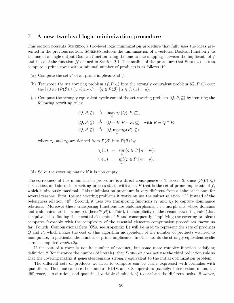
7 A new two-level logic minimization procedure

This section presents SCHERZO, a two-level logic minimization procedure that fully uses the ideas pre-sented in the previous section. SCHERZO reduces the minimization of a vectorial Boolean function f tothe one of a single-output Boolean function using the one-to-one mapping between the implicants of fand those of the function ff defined in Section 2.1. The outline of the procedure that SCHERZO uses tocompute a prime cover with a minimal number of products is as follows [19].

(a) Compute the set P of all prime implicants of f .

(b) Transpose the set covering problem 〈f, P,∈〉 into the strongly equivalent problem 〈Q,P,⊆〉 overthe lattice (P(B),⊆), where Q = q ∈ P(B) | x ∈ f, x = q.

(c) Compute the strongly equivalent cyclic core of the set covering problem 〈Q,P,⊆〉 by iterating thefollowing rewriting rules:

〈Q,P,⊆〉 1→ 〈max⊆

τP (Q), P,⊆〉,

〈Q,P,⊆〉 2→ 〈Q− E,P − E,⊆〉 with E = Q ∩ P,

〈Q,P,⊆〉 3→ 〈Q,max⊆

τQ(P ),⊆〉

where τP and τQ are defined from P(B) into P(B) by

τQ(w) = sup⊆

q ∈ Q | q ⊆ w,

τP (w) = inf⊆p ∈ P | w ⊆ p.

(d) Solve the covering matrix if it is non empty.

The correctness of this minimization procedure is a direct consequence of Theorem 3, since (P(B),⊆)is a lattice, and since the rewriting process starts with a set P that is the set of prime implicants of f ,which is obviously maximal. This minimization procedure is very different from all the other ones forseveral reasons. First, the set covering problems it works on use the subset relation “⊆” instead of thebelongness relation “∈”. Second, it uses two transposing functions τP and τQ to capture dominancerelations. Moreover these transposing functions are endomorphisms, i.e., morphisms whose domainsand codomains are the same set (here P(B)). Third, the simplicity of the second rewriting rule (thatis equivalent to finding the essential elements of P and consequently simplifying the covering problem)compares favorably with the complexity of the essential elements computation procedures known sofar. Fourth, Combinational Sets (CSs, see Appendix B) will be used to represent the sets of productsQ and P , which makes the cost of this algorithm independent of the number of products we need tomanipulate, in particular the number of prime implicants. In other words the strongly equivalent cycliccore is computed implicitly.

If the cost of a cover is not its number of product, but some more complex function satisfyingdefinition 2 (for instance the number of literals), then SCHERZO does not use the third reduction rule sothat the covering matrix it generates remains strongly equivalent to the initial optimization problem.

The different sets of products we need to compute can be easily expressed with formulas withquantifiers. Thus one can use the standart BDDs and CSs operators (namely: intersection, union, setdifference, substitution, and quantified variable elimination) to perform the different tasks. However,

26

this direct approach is not interesting from the computational point of view, because substitutions andquantified variable eliminations do not have a polynomial cost.

All the algorithms presented in the sequel are based on quantifier free recursive equations. Thesealgorithms use a divide and conquer strategy based on canonical decompositions of Boolean functionsand of sets of products. These decompositions are outlined in Section 7.1. BDDs and CSs describedin Appendices A and B are graph data structures based on these canonical decompositions. Thisyields a straighforward implementation. For the sake of clarity, the algorithms will be described onexplicit sets of products, since they can be directly translated into implicit manipulations of sets ofproducts, by replacing sets of products with their CSs, and set operations with their correspondentgraph combinators. All these algorithms use caches to avoid redundant computations, but we omittedthe cache look up for the sake of legibility.

We now explain how to perform the required computations by taking full advantage of the BDD andCS data structure, namely: computing all the prime implicants; computing q ∈ P(B) | x ∈ f, x = q;computing max⊆ τP (Q); and computing max⊆ τQ(P ).

7.1 Implicit prime implicant computation

Let P be a set of products built on the product space L =∏

k Lk, and lk be a literal (i.e., a subsetof Lk). We denote Plk the set of products p | lk · p ∈ P. We can canonically decompose P asP =

⋃

lk⊆Lklk ⊗ Plk , where P ⊗Q = p · q | p ∈ P, q ∈ Q. In the case where the product space in B,

we have

P = P1k ∪ xk ⊗ Pxk∪ xk ⊗ Pxk

.

For instance, if P = x1x4, x2, x2x4, x2x3 we have : P12 = x1x4; Px2= x3; Px2

= 1, x4. A setof products built on B is completely and uniquely defined by its three components P1k , Pxk

, and Pxk,

which founds the divide and conquer computation strategy.

Theorem 4 . Let f be a subset of L =∏

k Lk, and lk a literal. We denote flk the largest subset of∏

j 6=k Lj such that lk · flk ⊆ f . We have for any literal lk

Prime(f)lk = Prime(flk)−⋃

l′k⊇lk

l′k6=lk

Prime(fl′k

).

Proof. Let us note Impl(f) the set of implicants of f . By definition of flk , it is clear that for any subsetp of

∏

j 6=k Lj , the proposition lk ·p ⊆ f is equivalent to p ⊆ flk . This proves that Impl(f)lk = Impl(flk).A product p belongs to Prime(f)lk iff the two following properties are satisfied: (1) it is an implicant

of flk , and (2) lk · p is not contained by some other prime implicant of f . Thus p must belong toPrime(flk), and satisfy (2). To falsify (2), one must find a prime implicant of f containing lk · p, whichimplies that this prime implicant must be written as l′k · p′, with l′k ⊇ lk and p′ ⊇ p, and p′ ∈ Impl(fl′

k

).

First, note that we cannot have l′k = lk, for if this would mean that p is not maximal in Impl(flk).Second, if l′k ⊇ lk and l′k 6= lk, the only way for the prime implicant l′k · p′ of f to contain lk · p where pis maximal in Impl(flk) is to have p′ = p. This concludes the proof. 2

It is clear that flk =⋂

xk∈lkfxk. Applying the result above to the particular case of a total Boolean

function f defined on B, we obtain

Prime(f)1k = Prime(fxk∩ fxk

),

P rime(f)xk= Prime(fxk

)− Prime(f)1k ,

P rime(f)xk= Prime(fxk

)− Prime(f)1k .

27

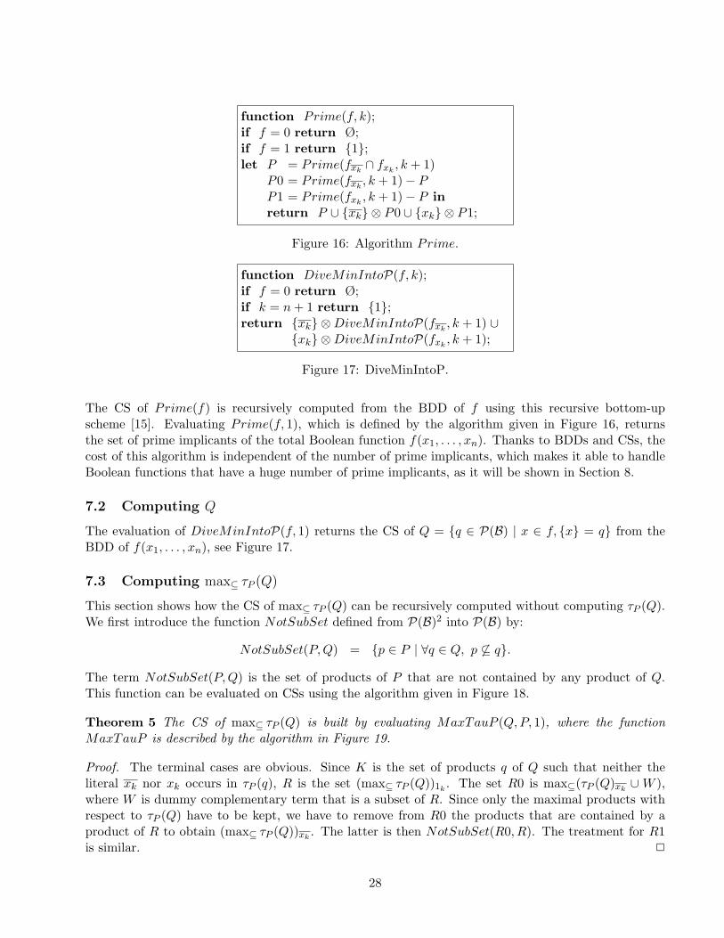
function Prime(f, k);if f = 0 return Ø;if f = 1 return 1;let P = Prime(fxk

∩ fxk, k + 1)

P0 = Prime(fxk, k + 1)− P

P1 = Prime(fxk, k + 1)− P in

return P ∪ xk ⊗ P0 ∪ xk ⊗ P1;

Figure 16: Algorithm Prime.

function DiveMinIntoP(f, k);if f = 0 return Ø;if k = n+ 1 return 1;return xk ⊗DiveMinIntoP(fxk

, k + 1) ∪xk ⊗DiveMinIntoP(fxk

, k + 1);

Figure 17: DiveMinIntoP.

The CS of Prime(f) is recursively computed from the BDD of f using this recursive bottom-upscheme [15]. Evaluating Prime(f, 1), which is defined by the algorithm given in Figure 16, returnsthe set of prime implicants of the total Boolean function f(x1, . . . , xn). Thanks to BDDs and CSs, thecost of this algorithm is independent of the number of prime implicants, which makes it able to handleBoolean functions that have a huge number of prime implicants, as it will be shown in Section 8.

7.2 Computing Q

The evaluation of DiveMinIntoP(f, 1) returns the CS of Q = q ∈ P(B) | x ∈ f, x = q from theBDD of f(x1, . . . , xn), see Figure 17.

7.3 Computing max⊆ τP (Q)

This section shows how the CS of max⊆ τP (Q) can be recursively computed without computing τP (Q).We first introduce the function NotSubSet defined from P(B)2 into P(B) by:

NotSubSet(P,Q) = p ∈ P | ∀q ∈ Q, p 6⊆ q.

The term NotSubSet(P,Q) is the set of products of P that are not contained by any product of Q.This function can be evaluated on CSs using the algorithm given in Figure 18.

Theorem 5 The CS of max⊆ τP (Q) is built by evaluating MaxTauP (Q,P, 1), where the functionMaxTauP is described by the algorithm in Figure 19.

Proof. The terminal cases are obvious. Since K is the set of products q of Q such that neither theliteral xk nor xk occurs in τP (q), R is the set (max⊆ τP (Q))1k . The set R0 is max⊆(τP (Q)xk

∪ W ),where W is dummy complementary term that is a subset of R. Since only the maximal products withrespect to τP (Q) have to be kept, we have to remove from R0 the products that are contained by aproduct of R to obtain (max⊆ τP (Q))xk

. The latter is then NotSubSet(R0, R). The treatment for R1is similar. 2

28

function NotSubSet(P,Q, k);if Q = Ø return P ;if P = Ø or 1 ∈ Q return Ø;if P = 1 return 1;return NotSubSet(P1k , Q1k , k + 1) ∪

xk ⊗NotSubSet(Pxk, Q1k ∪Qxk

, k + 1) ∪xk ⊗NotSubSet(Pxk

, Q1k ∪Qxk, k + 1);

Figure 18: Algorithm NotSubSet.

function MaxTauP (P,Q, k);if P = Ø or Q = Ø return Ø;if P = 1 return 1;if 1 /∈ P and Q = 1 return Ø;let K = Q1k ∪NotSubSet(Qxk

, Pxk) ∪NotSubSet(Qxk

, Pxk);

R = MaxTauP (P1k ,K, k + 1);R0 = MaxTauP (P1k ∪ Pxk

, Qxk, k + 1);

R1 = MaxTauP (P1k ∪ Pxk, Qxk

, k + 1) inreturn R ∪

xk ⊗NotSubSet(R0, R) ∪xk ⊗NotSubSet(R1, R);

Figure 19: Algorithm MaxTauP .

7.4 Computing max⊆ τQ(P )

This section shows how a recursive evaluation scheme directly produces the CS of max⊆ τQ(P ). We firstintroduce the function SupSet defined from P(B)2 into P(B) by

SupSet(P,Q) = p ∈ P | ∃q ∈ Q, q ⊆ p.

The term SupSet(P,Q) is the set of products of P that contain at least one product of Q. This functioncan be evaluated on CSs using the algorithm in Figure 20.

Theorem 6 The CS of max⊆ τQ(P ) is built by evaluating MaxTauQ(Q,P, 1), where the functionMaxTauQ is described by the algorithm in Figure 21.

function SupSet(P,Q, k);if P = Ø or Q = Ø return Ø;if P = 1 return 1;if 1 /∈ P and Q = 1 return Ø;return SupSet(P1k , Q1k ∪Qxk

∪Qxk, k + 1) ∪

xk ⊗ SupSet(Pxk, Qxk

, k + 1) ∪xk ⊗ SupSet(Pxk

, Qxk, k + 1);

Figure 20: Algorithm SupSet.

29

function MaxTauQ(Q,P, k);if Q = Ø or P = Ø return Ø;if 1 ∈ Q and 1 ∈ P return 1;let K = SupSet(P1k , Q1k) ∪

(SupSet(P1k , Qxk) ∩ SupSet(P1k , Qxk

));R = MaxTauQ(Q1k ∪Qxk

∪Qxk,K, k + 1);

R0 = MaxTauQ(Qxk, P1k ∪ Pxk

, k + 1);R1 = MaxTauQ(Qxk

, P1k ∪ Pxk, k + 1) in

return R ∪xk ⊗NotSubSet(R0, R) ∪xk ⊗NotSubSet(R1, R);

Figure 21: Algorithm MaxTauQ.

Proof. The terminal cases are obvious. By definition K is the set of products of P1k that contain aproduct of Q1k , or that contain a product of Qxk

and a product of Qxk. This means that K is the set

of products p of P such that τQ(p) does not contain the literal xk nor xk. The set R is then the set ofproducts of max⊆ τQ(P ) that do not contain the literal xk or xk.

It remains to compute the set of maximal sets of τQ(P ) that contain either the literal xk or theliteral xk. The set R0 is the set of products of τQ(P ) that contain the literal xk, and that are maximalwith respect to τQ(P )xk

. In addition with them, R0 includes other products containing the literal xk,which belongs to τQ(P ), but which are not maximal with respect to products of the set max⊆ τQ(P ).Since only the maximal products with respect to τQ(P ) have to be kept, i.e., the set NotSubSet(R0, R).A similar proof shows that NotSubSet(R1, R) is the subset of products of max⊆ τQ(P ) that contain theliteral xk. 2

7.5 Improvements for solving the covering matrix

Once SCHERZO has produced the two CSs that implicitely represent the covering matrix (indeed thecylic core if the cost function is the number of products), it solves it using a branch and bound algorithmthat switches from the CS representation to an explicit representation when the set covering problemis small enough (roughly less than 20 000 products). However the branch and bound algorithm usedby SCHERZO differs from the one used by ESPRESSO-EXACT and ESPRESSO-SIGNATURE by two importantimprovements that are presented in the next two sections.

Let C = 〈X,Y,∈〉 be a set covering problem. If the cyclic core of C is not empty, we choose anelement y as described in Section 3.3.1, and generate two new set covering problems, the first one definedas Cl = 〈X − y, Y − y,∈〉 that assumes that y belongs to the minimal solution, and the second onedefined by Cr = 〈X,Y − y,∈〉 that assumes that y does not belong to the minimal solution. Fora set covering problem C generated at some point of this binary search tree, we note C.min the costof its minimal solution, C.lower a lower bound of C.min computed thanks to an independent set (seeSection 3.3.2), and C.path the cost of the path that yields C, i.e., the sum of the costs of all y’s that havebeen assumed to belong to the minimal solution before reaching C. We note C.upper the global upperbound, i.e., the cost of the best global solution found so far. We ensure that C.path+C.lower < C.upperis always true, if not, the corresponding branch of root C is pruned, as it is done in ESPRESSO-EXACT.

30

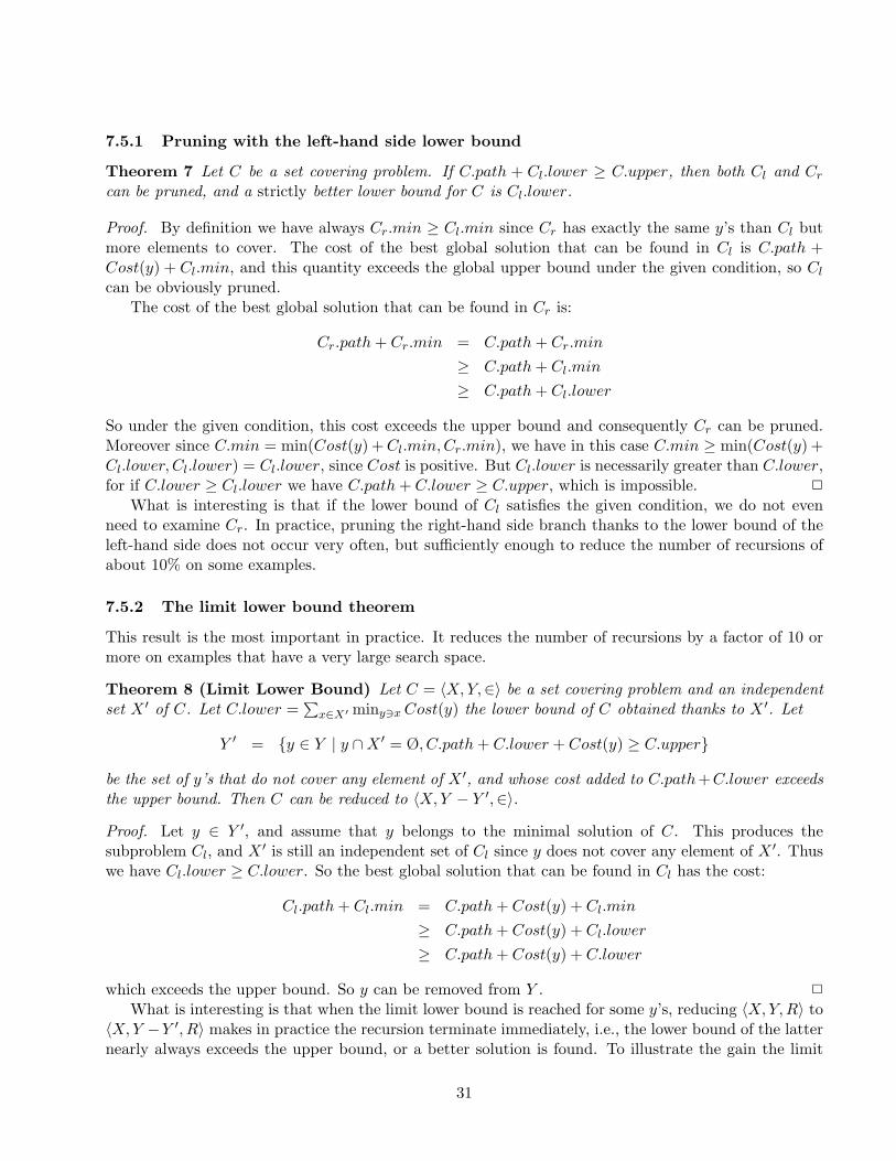
7.5.1 Pruning with the left-hand side lower bound

Theorem 7 Let C be a set covering problem. If C.path + Cl.lower ≥ C.upper, then both Cl and Cr

can be pruned, and a strictly better lower bound for C is Cl.lower.

Proof. By definition we have always Cr.min ≥ Cl.min since Cr has exactly the same y’s than Cl butmore elements to cover. The cost of the best global solution that can be found in Cl is C.path +Cost(y) + Cl.min, and this quantity exceeds the global upper bound under the given condition, so Cl

can be obviously pruned.The cost of the best global solution that can be found in Cr is:

Cr.path+ Cr.min = C.path+ Cr.min

≥ C.path+ Cl.min

≥ C.path+ Cl.lower

So under the given condition, this cost exceeds the upper bound and consequently Cr can be pruned.Moreover since C.min = min(Cost(y) +Cl.min, Cr.min), we have in this case C.min ≥ min(Cost(y) +Cl.lower, Cl.lower) = Cl.lower, since Cost is positive. But Cl.lower is necessarily greater than C.lower,for if C.lower ≥ Cl.lower we have C.path+ C.lower ≥ C.upper, which is impossible. 2

What is interesting is that if the lower bound of Cl satisfies the given condition, we do not evenneed to examine Cr. In practice, pruning the right-hand side branch thanks to the lower bound of theleft-hand side does not occur very often, but sufficiently enough to reduce the number of recursions ofabout 10% on some examples.

7.5.2 The limit lower bound theorem

This result is the most important in practice. It reduces the number of recursions by a factor of 10 ormore on examples that have a very large search space.

Theorem 8 (Limit Lower Bound) Let C = 〈X,Y,∈〉 be a set covering problem and an independentset X ′ of C. Let C.lower =

∑

x∈X′ miny∋xCost(y) the lower bound of C obtained thanks to X ′. Let

Y ′ = y ∈ Y | y ∩X ′ = Ø, C.path+ C.lower + Cost(y) ≥ C.upper

be the set of y’s that do not cover any element of X ′, and whose cost added to C.path+C.lower exceedsthe upper bound. Then C can be reduced to 〈X,Y − Y ′,∈〉.

Proof. Let y ∈ Y ′, and assume that y belongs to the minimal solution of C. This produces thesubproblem Cl, and X ′ is still an independent set of Cl since y does not cover any element of X ′. Thuswe have Cl.lower ≥ C.lower. So the best global solution that can be found in Cl has the cost:

Cl.path+ Cl.min = C.path+ Cost(y) + Cl.min

≥ C.path+ Cost(y) + Cl.lower

≥ C.path+ Cost(y) + C.lower

which exceeds the upper bound. So y can be removed from Y . 2

What is interesting is that when the limit lower bound is reached for some y’s, reducing 〈X,Y,R〉 to〈X,Y −Y ′, R〉 makes in practice the recursion terminate immediately, i.e., the lower bound of the latternearly always exceeds the upper bound, or a better solution is found. To illustrate the gain the limit

31

lower bound produces, assume that Cost(y) = 1 for all y. Then instead of terminating the recursionwhen the global lower bound (i.e., C.path+C.lower) reaches C.upper, it is nearly always pruned whenthe global lower bound reaches C.upper − 1. This gain of 1 in the depth of the search can produce anexponential reduction of the space search and reduces dramatically the exploration time. This effect iseven more significant when dealing with more discriminant cost functions, for instance cost functionsthat depend on the literals.

The use of the limit lower bound enables us to solve or improve the best known solutions of someunsolved cyclic cores4, and to reduce dramatically the time needed to explore the search space: the gainin CPU time is more than 10 on some examples.

7.6 Conclusion

We have presented a two-level logic minimization algorithm that is based on rewriting rules withinthe lattice (P(B),⊆) [19]. These transposing function based transformations produce a set coveringproblem strongly equivalent to the cyclic core of the Boolean function to minimize. They also allow theuse of the efficient CS data structure all along the computation. The effectiveness of CSs to implicitlyrepresent sets of products makes the complexity of this algorithm independent from the number ofminterms and prime implicants of f , and the uniformization of the workspace to the lattice (P(B),⊆)makes this algorithm able to handle problems that are out of reach of any other technique known so far(see Section 8).

In the case when the (strongly equivalent) cyclic core of the Boolean function f to be minimizedis empty, a minimal prime cover of f can be immediately built by choosing, for each of the es-sential elements that have been discovered during the fixpoint computation, a prime implicant of fwith a minimal cost that contains it. It is interesting to note that if the cost function has the formCost(l1 · · · ln) = c1(l1) ∗ c2(l2) ∗ · · · ∗ cn(ln), where ∗ is any associative operator and lk’s are literals, thenextracting from a set of products P the products that minimize the cost function can be done with acomplexity linear with respect to the size of the CS representing P [18].

In the case when the cyclic core is not empty, a branch-and-bound algorithm is used to solve it. Itmixes both implicite CS based techniques and explicite techniques. Its efficiency comes mainly fromthe use of the limit lower bound that dramatically reduces the search space.

8 Experimental results

We compare 3 two-level logic minimization methods. The first one is ESPRESSO-EXACT [57], based onthe Quine–McCluskey procedure presented in Section 3. The second one is ESPRESSO-SIGNATURE, thesignature cube based method [7] presented in Section 5. The third one [19] is SCHERZO, described inSection 7.

There are two reasons for which ESPRESSO-EXACT can fail in minimizing a function. Either thenumber of prime implicants is too large to be computed explicitly, or the set covering problem ESPRESSO-

EXACT generates is too complex to be solved. Note that if ESPRESSO-EXACT can minimize a function,then ESPRESSO-SIGNATURE can too, since the latter generates smaller covering. However ESPRESSO-

SIGNATURE is still limited by the number of maximal signature cubes. SCHERZO generates two graphs,namely CSs, that implicitely represent a strongly equivalent covering matrix (this matrix is strongly

4For the MCNC benchmark [68], a solution of size 65 (instead of 67) has been found for ex5, 259 (instead of 261) formax1024, 122 (instead of 125) for bench1, 100 (instead of 104) for test4, and 477 (instead of 491) for test3.

32

equivalent to the cyclic core when the cost function is the number of products). The advantage is thatSCHERZO is not limited by the size of the covering matrix.

Any function that can be minimized with ESPRESSO-SIGNATURE can also be minimized by SCHERZO,providing that one can build the BDD of the function and the CS of its prime implicants. As far aswe looked from the theorical point of view, nothing prevents the existence of a function that could betreated by ESPRESSO-SIGNATURE but not by SCHERZO: a function with a polynomial sum-of-productsrepresentation but that has an exponential

BDD representation would be such an example. However it is not clear whether such a function canstill have a polynomial number of maximal signature cubes. So far we have not found such a counterexample.

Among the 134 examples of the MCNC benchmark [68] that describe partial vectorial Booleanfunctions, ESPRESSO-EXACT cannot compute explicitly the prime implicants of 17 of them, and 3 areunsolved though their covering matrices have been built. The 114 examples ESPRESSO-EXACT can solveare the “easy” examples. For solving the 114 “easy” examples on a DEC 5000, ESPRESSO-EXACT takes9264 seconds [59], ESPRESSO-SIGNATURE 7777 seconds [59], and SCHERZO requires 471 seconds. The CPUtime measured for SCHERZO includes: reading the file, building the BDDs of the function ff described inSection 2.1 (its variable ordering is determined with the help of the heuristics introduced in [67] and the“sifting” technique [58]), minimizing ff , and recovering the original solution. The most time consumingoperation of consists of building the BDDs of ff and computing implicitly its cyclic core. This processis especially costly when dynamic variable ordering is necessary. On these “easy” examples SCHERZO is16 times faster than ESPRESSO-SIGNATURE and 19 times faster than ESPRESSO-EXACT. Table 1 shows theCPU time in seconds on a DEC 5000 to minimize 33 of these examples that represent about 90% of thecumulated time for solving the 114 easy examples. On these “easy” examples, most of the efficiency ofSCHERZO comes from the use of the limit lower bound.

The remaining 20 “hard” examples, in addition with 3 other examples on which ESPRESSO-EXACT

fails, are known as the 23 hard ESPRESSO-EXACT examples. Table 2 gives the characteristic of the hardESPRESSO-EXACT examples. We clearly see that the algorithm presented Section 7.1 is not limited bythe huge number of prime implicants of some functions, thanks to the implicit representation of sets ofproducts it uses. For instance the CS of the 1.12 e+15 prime implicants of mish is computed in 0.3seconds on a DEC 5000, and it has only 2435 vertices. A “?” in column B indicates that it is onlyan upper bound on the minimal sum-of-products, obtained thanks to an irredundant prime cover thathas not been proven as minimal. A “∗” indicates an improvement due to SCHERZO, either by solving apreviously open problem, or by providing with a better solution that the one known so far.

Table 3 compares the results of ESPRESSO-SIGNATURE reported in [36] and those of SCHERZO onthe hard espresso examples. Column row × col give the number of rows and columns of the coveringmatrix that is produced by both methods. For ESPRESSO-SIGNATURE, the number of rows is the numberof maximal signature cubes, and the number of columns is the number of prime implicants that containa maximal signature cube. For SCHERZO, it is the size of the cyclic core. Column Tmatrix gives theCPU time that ESPRESSO-SIGNATURE needs to generate the covering matrix. Column Tcc gives theCPU time that SCHERZO needs to implicitely compute the cyclic core. A “na” indicates a non availabledatum. A “−” indicates that the computation failed at the step given by the column when it occurs.

The size of the matrix SCHERZO produces is obviously smaller than the one generated by ESPRESSO-

SIGNATURE since the latter does not compute directly the cyclic core. SCHERZO is able to generatethe cyclic core of all examples, while ESPRESSO-SIGNATURE is sometimes unable to generate a coveringmatrix because of a too large number of maximal signature cubes. For instance, mainpla, soar, and ti

33

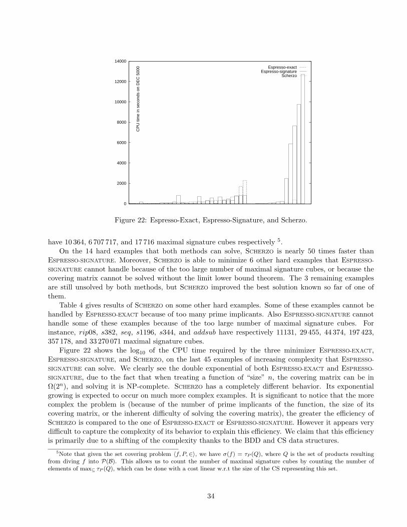
0

2000

4000

6000

8000

10000

12000

14000

CP

U ti

me

in s

econ

ds o

n D

EC

500

0 Espresso-exactEspresso-signature

Scherzo

Figure 22: Espresso-Exact, Espresso-Signature, and Scherzo.

have 10 364, 6 707 717, and 17 716 maximal signature cubes respectively 5.On the 14 hard examples that both methods can solve, SCHERZO is nearly 50 times faster than

ESPRESSO-SIGNATURE. Moreover, SCHERZO is able to minimize 6 other hard examples that ESPRESSO-

SIGNATURE cannot handle because of the too large number of maximal signature cubes, or because thecovering matrix cannot be solved without the limit lower bound theorem. The 3 remaining examplesare still unsolved by both methods, but SCHERZO improved the best solution known so far of one ofthem.

Table 4 gives results of SCHERZO on some other hard examples. Some of these examples cannot behandled by ESPRESSO-EXACT because of too many prime implicants. Also ESPRESSO-SIGNATURE cannothandle some of these examples because of the too large number of maximal signature cubes. Forinstance, rip08, s382, seq, s1196, s344, and addsub have respectively 11131, 29 455, 44 374, 197 423,357 178, and 33 270 071 maximal signature cubes.

Figure 22 shows the log10 of the CPU time required by the three minimizer ESPRESSO-EXACT,ESPRESSO-SIGNATURE, and SCHERZO, on the last 45 examples of increasing complexity that ESPRESSO-

SIGNATURE can solve. We clearly see the double exponential of both ESPRESSO-EXACT and ESPRESSO-

SIGNATURE, due to the fact that when treating a function of “size” n, the covering matrix can be inΩ(2n), and solving it is NP-complete. SCHERZO has a completely different behavior. Its exponentialgrowing is expected to occur on much more complex examples. It is significant to notice that the morecomplex the problem is (because of the number of prime implicants of the function, the size of itscovering matrix, or the inherent difficulty of solving the covering matrix), the greater the efficiency ofSCHERZO is compared to the one of ESPRESSO-EXACT or ESPRESSO-SIGNATURE. However it appears verydifficult to capture the complexity of its behavior to explain this efficiency. We claim that this efficiencyis primarily due to a shifting of the complexity thanks to the BDD and CS data structures.

5Note that given the set covering problem 〈f, P,∈〉, we have σ(f) = τP (Q), where Q is the set of products resultingfrom diving f into P(B). This allows us to count the number of maximal signature cubes by counting the number ofelements of max⊆ τP (Q), which can be done with a cost linear w.r.t the size of the CS representing this set.

34

9 Conclusion

Two-level logic minimization is a well known problem of computer science that applies in logic synthe-sis, reliability analysis, and automated reasoning. This paper gave an overview of the methods thathave been proposed to solve this problem. We presented the widely used Quine–McCluskey algorithm(ESPRESSO-EXACT), that is limited by the number of prime implicants of the Boolean function to beminimized. We introduced new concepts to establish transformations of the minimization problem intosome other ones, in which good properties can be exploited to yield an original minimization algorithm.A good example is the signature cube based minimization method (ESPRESSO-SIGNATURE) that does notnecessarily require the computation of all prime implicants. Going further we studied how to solve setcovering problems over lattices by exploiting the properties of lattices, and by using transformationsthat preserve the structure of the problem. The application of this essential result to two-level logicminimization yields the new minimization procedure SCHERZO. First, this algorithm is no longer lim-ited by the number of prime implicants thanks to the use of efficient graph representations of Booleanfunctions and sets of products. Second, it fully exploits isomorphic transformations of sets coveringproblems whithin the same workspace, namely the complete lattice made of products and the subsetrelation. Third, it improves the branch and bound technique thanks to the limit lower bound theoremthat dramatically reduces the number of recursions. These techniques enables SCHERZO to be signifi-cantly faster than the best methods known so far, and allows the two-level minimization of functionsthat are out of reach of any other algorithm.

Acknowledgment

The author would like to thank Anna Karlin, Herve Touati, and the reviewers for their constructivecomments on the early draft of this paper. SCHERZO has been developed with the TiGeR library writtenby Jean Christophe Madre, Herve Touati, and the author.

A Binary Decision Diagrams

Several normal forms of Propositional Logic have been used in the past as the basis of automatedpropositional provers and constraint solvers. Some of these normal forms have the remarkable propertyof being canonical. These canonical forms are very appealing because they support very simple proofprocedures. Two formulas written in canonical form are equivalent if and only if they are syntacticallyequal.

The computational cost of a proof procedure based on canonical rewriting depends on the timeneeded to rewrite the formula to be proved valid into its canonical form. This time is in the worst case,for all canonical forms, exponential with respect to the size of the formula to be rewritten. The problemis that this worst case was very easily obtained for all the canonical forms that were known until veryrecently.

Binary decision diagrams (BDDs) are a graph based canonical representation of Boolean functionsthat is widely used in CAD for verification and synthesis [11]. This representation is strongly relatedto Boole’s expansion theorem [5], also called Shannon decomposition since his work on switching func-tions [61]. The Shannon decomposition6 of a total Boolean function f with respect to a variable x isthe couple of functions (fx, fx) [5] such that: f = xfx + xfx. When iterated for all the variables of

6This is a particular case of the decomposition given Section 7.1

35

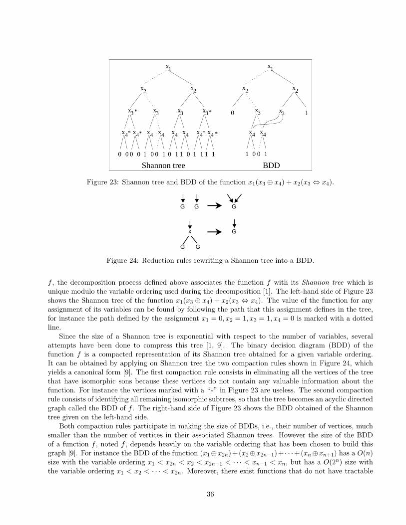
Shannon tree BDD

0 0

x4 x4

x3

1 1 0

x4 x4

* x3

1

x4 x4* *

x3

1 1 1 10 0 0 0

x4 x4* *

x3 *

x2 x2

x1

0 0

x4 x4

x3

1 1

x3 10

x2 x2

x1

1 0

Figure 23: Shannon tree and BDD of the function x1(x3 ⊕ x4) + x2(x3 ⇔ x4).

G G G

x

G G

G

Figure 24: Reduction rules rewriting a Shannon tree into a BDD.

f , the decomposition process defined above associates the function f with its Shannon tree which isunique modulo the variable ordering used during the decomposition [1]. The left-hand side of Figure 23shows the Shannon tree of the function x1(x3 ⊕ x4) + x2(x3 ⇔ x4). The value of the function for anyassignment of its variables can be found by following the path that this assignment defines in the tree,for instance the path defined by the assignment x1 = 0, x2 = 1, x3 = 1, x4 = 0 is marked with a dottedline.

Since the size of a Shannon tree is exponential with respect to the number of variables, severalattempts have been done to compress this tree [1, 9]. The binary decision diagram (BDD) of thefunction f is a compacted representation of its Shannon tree obtained for a given variable ordering.It can be obtained by applying on Shannon tree the two compaction rules shown in Figure 24, whichyields a canonical form [9]. The first compaction rule consists in eliminating all the vertices of the treethat have isomorphic sons because these vertices do not contain any valuable information about thefunction. For instance the vertices marked with a “∗” in Figure 23 are useless. The second compactionrule consists of identifying all remaining isomorphic subtrees, so that the tree becomes an acyclic directedgraph called the BDD of f . The right-hand side of Figure 23 shows the BDD obtained of the Shannontree given on the left-hand side.

Both compaction rules participate in making the size of BDDs, i.e., their number of vertices, muchsmaller than the number of vertices in their associated Shannon trees. However the size of the BDDof a function f , noted f , depends heavily on the variable ordering that has been chosen to build thisgraph [9]. For instance the BDD of the function (x1⊕x2n)+(x2⊕x2n−1)+ · · ·+(xn⊕xn+1) has a O(n)size with the variable ordering x1 < x2n < x2 < x2n−1 < · · · < xn−1 < xn, but has a O(2n) size withthe variable ordering x1 < x2 < · · · < x2n. Moreover, there exist functions that do not have tractable

36

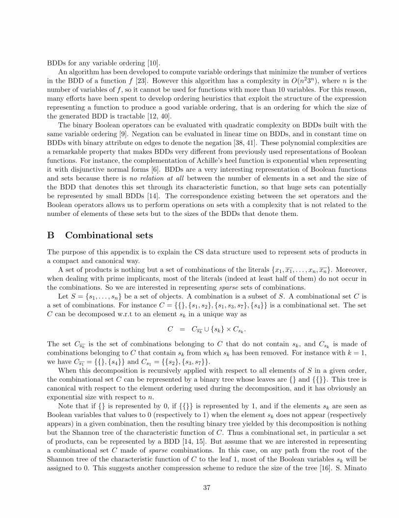
BDDs for any variable ordering [10].An algorithm has been developed to compute variable orderings that minimize the number of vertices

in the BDD of a function f [23]. However this algorithm has a complexity in O(n23n), where n is thenumber of variables of f , so it cannot be used for functions with more than 10 variables. For this reason,many efforts have been spent to develop ordering heuristics that exploit the structure of the expressionrepresenting a function to produce a good variable ordering, that is an ordering for which the size ofthe generated BDD is tractable [12, 40].

The binary Boolean operators can be evaluated with quadratic complexity on BDDs built with thesame variable ordering [9]. Negation can be evaluated in linear time on BDDs, and in constant time onBDDs with binary attribute on edges to denote the negation [38, 41]. These polynomial complexities area remarkable property that makes BDDs very different from previously used representations of Booleanfunctions. For instance, the complementation of Achille’s heel function is exponential when representingit with disjunctive normal forms [6]. BDDs are a very interesting representation of Boolean functionsand sets because there is no relation at all between the number of elements in a set and the size ofthe BDD that denotes this set through its characteristic function, so that huge sets can potentiallybe represented by small BDDs [14]. The correspondence existing between the set operators and theBoolean operators allows us to perform operations on sets with a complexity that is not related to thenumber of elements of these sets but to the sizes of the BDDs that denote them.

B Combinational sets

The purpose of this appendix is to explain the CS data structure used to represent sets of products ina compact and canonical way.

A set of products is nothing but a set of combinations of the literals x1, x1, . . . , xn, xn. Moreover,when dealing with prime implicants, most of the literals (indeed at least half of them) do not occur inthe combinations. So we are interested in representing sparse sets of combinations.

Let S = s1, . . . , sn be a set of objects. A combination is a subset of S. A combinational set C isa set of combinations. For instance C = , s1, s2, s1, s3, s7, s4 is a combinational set. The setC can be decomposed w.r.t to an element sk in a unique way as

C = Csk ∪ sk × Csk .

The set Csk is the set of combinations belonging to C that do not contain sk, and Csk is made ofcombinations belonging to C that contain sk from which sk has been removed. For instance with k = 1,we have Cs1 = , s4 and Cs1 = s2, s3, s7.

When this decomposition is recursively applied with respect to all elements of S in a given order,the combinational set C can be represented by a binary tree whose leaves are and . This tree iscanonical with respect to the element ordering used during the decomposition, and it has obviously anexponential size with respect to n.

Note that if is represented by 0, if is represented by 1, and if the elements sk are seen asBoolean variables that values to 0 (respectively to 1) when the element sk does not appear (respectivelyappears) in a given combination, then the resulting binary tree yielded by this decomposition is nothingbut the Shannon tree of the characteristic function of C. Thus a combinational set, in particular a setof products, can be represented by a BDD [14, 15]. But assume that we are interested in representinga combinational set C made of sparse combinations. In this case, on any path from the root of theShannon tree of the characteristic function of C to the leaf 1, most of the Boolean variables sk will beassigned to 0. This suggests another compression scheme to reduce the size of the tree [16]. S. Minato

37

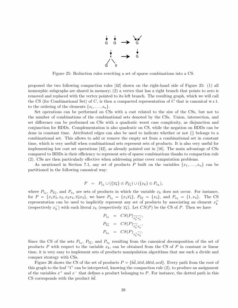
G G G

x

G

G

0

Figure 25: Reduction rules rewriting a set of sparse combinations into a CS.

proposed the two following compaction rules [42] shown on the right-hand side of Figure 25: (1) allisomorphic subgraphs are shared in memory; (2) a vertex that has a right branch that points to zero isremoved and replaced with the vertex pointed to its left branch. The resulting graph, which we will callthe CS (for Combinational Set) of C, is then a compacted representation of C that is canonical w.r.t.to the ordering of the elements s1, . . . , sn.

Set operations can be performed on CSs with a cost related to the size of the CSs, but not tothe number of combinations of the combinational sets denoted by the CSs. Union, intersection, andset difference can be performed on CSs with a quadratic worst case complexity, as disjunction andconjunction for BDDs. Complementation is also quadratic on CS, while the negation on BDDs can bedone in constant time. Attributed edges can also be used to indicate whether or not belongs to acombinational set. This allows to add or remove the empty set from a combinational set in constanttime, which is very usefull when combinational sets represent sets of products. It is also very useful forimplementing low cost set operations [42], as already pointed out in [16]. The main advantage of CSscompared to BDDs is their efficiency to represent sets of sparse combinations thanks to compaction rule(2). CSs are then particularly effective when addressing prime cover computation problems.

As mentioned in Section 7.1, any set of products P built on the variables x1, . . . , xn can bepartitioned in the following canonical way:

P = P1k ∪ (xk ⊗ Pxk) ∪ (xk ⊗ Pxk

),

where P1k , Pxk, and Pxk

are sets of products in which the variable xk does not occur. For instance,for P = x1x4, x2, x2x4, x2x3, we have P12 = x1x4, Px2

= x3, and Px2= 1, x4. The CS

representation can be used to implicitly represent any set of products by associating an element x+k(respectively x−k ) with each literal xk (respectively xk). Let CS(P ) be the CS of P . Then we have

P1k = CS(P )x+

kx−k

,

Pxk= CS(P )

x+

kx−k

,

Pxk= CS(P )

x+

kx−k

.

Since the CS of the sets P1k , Pxk, and Pxk

resulting from the canonical decomposition of the set ofproducts P with respect to the variable xk, can be obtained from the CS of P in constant or lineartime, it is very easy to implement sets of products manipulation algorithms that use such a divide andconquer strategy with CSs.

Figure 26 shows the CS of the set of products P = bd, acd, abcd, acd. Every path from the root ofthis graph to the leaf “1” can be interpreted, knowing the compaction rule (2), to produce an assignmentof the variables x+ and x− that defines a product belonging to P . For instance, the dotted path in thisCS corresponds with the product bd.

38

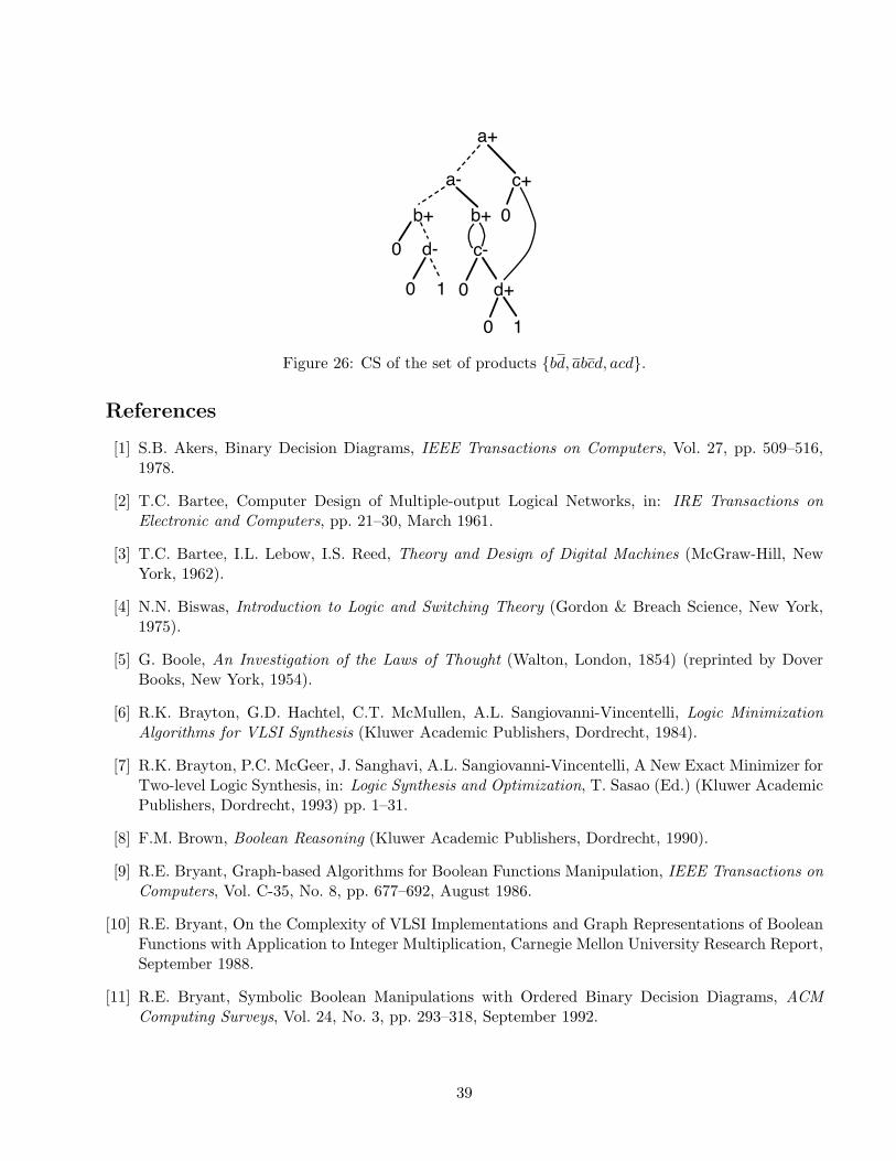
1

1

0

a+

a-

b+

c+

c-d-

b+

d+

0

0

0

0

Figure 26: CS of the set of products bd, abcd, acd.

References

[1] S.B. Akers, Binary Decision Diagrams, IEEE Transactions on Computers, Vol. 27, pp. 509–516,1978.

[2] T.C. Bartee, Computer Design of Multiple-output Logical Networks, in: IRE Transactions onElectronic and Computers, pp. 21–30, March 1961.

[3] T.C. Bartee, I.L. Lebow, I.S. Reed, Theory and Design of Digital Machines (McGraw-Hill, NewYork, 1962).

[4] N.N. Biswas, Introduction to Logic and Switching Theory (Gordon & Breach Science, New York,1975).

[5] G. Boole, An Investigation of the Laws of Thought (Walton, London, 1854) (reprinted by DoverBooks, New York, 1954).

[6] R.K. Brayton, G.D. Hachtel, C.T. McMullen, A.L. Sangiovanni-Vincentelli, Logic MinimizationAlgorithms for VLSI Synthesis (Kluwer Academic Publishers, Dordrecht, 1984).

[7] R.K. Brayton, P.C. McGeer, J. Sanghavi, A.L. Sangiovanni-Vincentelli, A New Exact Minimizer forTwo-level Logic Synthesis, in: Logic Synthesis and Optimization, T. Sasao (Ed.) (Kluwer AcademicPublishers, Dordrecht, 1993) pp. 1–31.

[8] F.M. Brown, Boolean Reasoning (Kluwer Academic Publishers, Dordrecht, 1990).

[9] R.E. Bryant, Graph-based Algorithms for Boolean Functions Manipulation, IEEE Transactions onComputers, Vol. C-35, No. 8, pp. 677–692, August 1986.

[10] R.E. Bryant, On the Complexity of VLSI Implementations and Graph Representations of BooleanFunctions with Application to Integer Multiplication, Carnegie Mellon University Research Report,September 1988.

[11] R.E. Bryant, Symbolic Boolean Manipulations with Ordered Binary Decision Diagrams, ACMComputing Surveys, Vol. 24, No. 3, pp. 293–318, September 1992.

39

[12] K.M. Butler, D.E. Ross, R. Kapur, M.R. Mercer, Heuristics to Compute Variable Orderings forEfficient Manipulations of Ordered Binary Decision Diagrams, Proc. 28th Design Automation Con-ference, pp. 417–420, San Francisco, California, June 1991.

[13] A.K. Chandra, G. Markowsky, On the Number of Prime Implicants, Discrete Mathematics, Vol. 24,pp. 7–11, 1978.

[14] O. Coudert, J.C. Madre, A New Method to Compute Prime and Essential Prime Implicants ofBoolean Functions, Proc. Brown/MIT Conference on Advanced Research in VLSI and ParallelSystems, Cambridge, MA, USA, March 1992.

[15] O. Coudert, J.C. Madre, Implicit and Incremental Computation of Primes and Essential Primesof Boolean Functions, Proc. 29th Design Automation Conference, Anaheim, CA, USA, pp. 36–39,June 1992.

[16] O. Coudert, J.C. Madre, A New Graph Based Prime Computation Technique, in Logic Synthesisand Optimization, T. Sasao (Ed.) (Kluwer Academic Publishers, Dordrecht, 1993) pp. 33–57.

[17] O. Coudert, J.C. Madre, Towards a Symbolic Logic Minimization Algorithm, Proc. VLSI Design,Bombay, India, January 1993.

[18] O. Coudert, J.C. Madre, Fault Tree Analysis: 1020 Prime Implicants and Beyond, Proc. AnnualReliability and Maintainability Symposium, Atlanta, GA, USA, pp. 240–245, January 1993.

[19] O. Coudert, J.C. Madre, H. Fraisse, A New Viewpoint on Two-Level Logic Minimization, Proc.30th Design Automation Conference, Dallas, TX, USA, pp. 625–630, June 1993.

[20] R.B. Cutler, S. Muroga, Useless Prime Implicants of Incompletely Specified Multiple-OutputSwitching Functions, International Journal of Computer and Information Sciences, Vol. 9, No. 4,1980.

[21] M. Davis, H. Putnam, A Computing Procedure for Quantification Theory, Journal of the ACM,Vol. 7, pp. 201–215, 1960.

[22] J. Doyle, A Truth Maintenance System, Artificial Intelligence, Vol. 12, pp. 231–271, 1979.

[23] S.J. Friedman, K.J. Supowit, Finding the Optimal Variable Ordering for Binary Decision Diagrams,IEEE Transactions on Computer, Vol. C-39, No. 5, pp. 710–713, May 1990.

[24] J.F. Gimpel, A Reduction Technique for Prime Implicant Tables, IEEE Transactions on ElectronicsComputers, Vol. EC-14, pp. 535–541, 1965.

[25] D.F. Hasl, Advanced Concepts in Fault Tree Analysis, Proc. System Safety Symposium, Seattle,USA, June 1965.

[26] S.J. Hong, R.G. Cain, D.L. Ostapko, MINI: A Heuristic Approach for Logic Minimization, IBMJournal R&D, pp. 443–458, 1974.

[27] S.J. Hong, S. Muroga, Absolute Minimization of Completely Specified Switching Functions, IEEETransactions on Computers, Vol. 40, pp. 53–65, 1991.

[28] H.R. Hwa, A Method for Generating Prime Implicants of a Boolean Expression, IEEE Transactionson Computers, pp. 637–641, June 1974.

40

[29] M. Karnaugh, The Map Method for Synthesis of Combinational Logic Circuits, AIEE Transactionson Communications & Electronics, Vol. 9, pp. 593–599, 1953.

[30] J. De Kleer, An Assumption-based TMS, Artificial Intelligence, Vol. 28, pp. 127–162, 1986.

[31] J. De Kleer, B.C. Williams, Diagnosing Multiple Faults, Artificial Intelligence, Vol. 32, pp. 97–130,1987.

[32] B. Lin, O. Coudert, J.C. Madre, Symbolic Prime Generation for Multiple-Valued Functions, Proc.29th Design Automation Conference, Anaheim, CA, USA, pp. 40–44, June 1992.

[33] M.C. Loui, G. Bilardi, The Correctness of Tison’s Method for Generating Prime Implicants, ReportR-952, UILU-ENG 82-2218, Coordinated Science Laboratory, University of Illinois at Urbana-Champaign, 1982.

[34] E.L. Jr. McCluskey, Minimization of Boolean Functions, Bell System Technical Journal, Vol. 35,pp. 1417–1444, April 1959.

[35] E.L. Jr. McCluskey, H. Schorr, Essential Multiple Output Prime Implicants, Proc. Symposium onMathematical Theory of Automata, Vol. 12, Polytechnic Institute of Brooklyn, New York, NY,pp. 437–457, April 1962.

[36] P.C. McGeer, J. Sanghavi, R.K. Brayton, A.L. Sangiovanni-Vincentelli, ESPRESSO-SIGNATURE: ANew Exact Minimizer fo Logic Functions, IEEE Transactions on VLSI, Vol. 1, No. 4, pp. 432–440,December 1993.

[37] C. McMullen, J. Shearer, Prime Implicants, Minimum Covers, and the Complexity of Logic Sim-plification, IEEE Transactions on Computers, Vol. C-35, pp. 761–762, August 1986.

[38] J.C. Madre, J.P. Billon, Proving Circuit Correctness using Formal Comparison Between Expectedand Extracted Behaviour, Proc. 25th Design Automation Conference, Anaheim, CA, USA, July1988.

[39] J.C. Madre, O. Coudert, A Logically Complete Reasoning Maintenance System Based on LogicalConstrain Solver, Proc. Int. Join Conference on Artificial Intelligence, Sydney, Australia, August1991.

[40] S. Malik, A.R. Wang, R.K. Brayton, A. Sangiovanni-Vincentelli, Logic Verification using BinaryDecision Diagrams in a Logic Synthesis Environment, Proc. Int. Conference on Computer AidedDesign, Santa Clara, USA, pp. 6–9, November 1988.

[41] S. Minato, N. Ishiura, S. Yajima, Fast Tautology Checking Using Shared Binary DecisionDiagrams—Experimental Results, in: Formal VLSI Correctness Verification, L.J.M. Claesen (Ed.)(North-Holland, Amsterdam, 1989) pp. 107–111.

[42] S. Minato, Zero-Supressed BDDs for Set Manipulation in Combinatorial Problems, Proc. 30thDesign Automation Conference, Dallas, TX, pp. 272–277, June 1993.

[43] E. Morreale, Recursive Operators for Prime Implicant and Irredundant Normal Form Determina-tion, IEEE Transactions on Computers, 1970.

[44] I.B. Pyne, E.L. McCluskey, An Essay on Prime Implicant Tables, SIAM, Vol. 9, pp. 604–632, 1961.

41

[45] W.V.O. Quine, The problem of Simplifying Truth Functions, American Mathematics Monthly, Vol.59, pp. 521–531, 1952.

[46] W.V.O. Quine, Two Theorems about Truth Functions, Bol. Society of Mathematics Mexicana, Vol.10, pp. 64–70, 1953.

[47] W.V.O. Quine, A Way to Simplify Truth Functions, American Mathematics Monthly, Vol. 62,pp. 627–631, 1955.

[48] W.V.O. Quine, On Cores and Prime Implicants of Truth Functions, American MathematicsMonthly, Vol. 66, pp. 755–760, 1959.

[49] R. Reiter, A Theory of Diagnosis From First Principles, Artificial Intelligence, Vol. 32, pp. 57–95,1987.

[50] R. Reiter, J. de Kleer, Foundations for Assumption-based Truth Maintenance Systems, Proc. AAAINational Conference’87, Seattle, pp. 183–188, July 1987.

[51] V.T. Rhyne, P.S. Noe, M.H. McKinney, U.W. Pooch, A New Technique for the Fast Minimizationof Switching Functions, IEEE Transactions on Computers, Vol. C-26, No. 8, pp. 757–764, 1977.

[52] J.A. Robinson, A Machine-oriented Logic Based on the Resolution Principle, Journal of ACM,Vol. 12, pp. 23–41, 1965.

[53] S. Robinson, R. House, Gimpel’s Reduction Technique Extended to the Covering Problem WithCosts, IEEE Transactions on Electronic Computer, Vol. EC-16, pp. 509–514, August 1967.

[54] J.P. Roth, Algebraic Topological Methods for the Synthesis of Switching Systems, Transactions ofAmerican Methematical Society, Vol. 88, No. 2, pp. 301–326, 1958.

[55] R.L. Rudell, Multiple-Valued Logic Minimization for PLA Synthesis, Research Report, UCBM86/65, 1986.

[56] R.L. Rudell, A.L. Sangiovanni-Vincentelli, Multiple Valued Minimization for PLA Optimization,IEEE Transactions on CAD, Vol. 6, No. 5, pp. 727–750, September 1987.

[57] R.L. Rudell, Logic Synthesis for VLSI Design, PhD Thesis, UCB/ERL M89/49, 1989.

[58] R.L. Rudell, Dynamic Variable Ordering for Binary Decision Diagrams, Proc. Int. Conference onComputer Aided Design, Santa Clara, USA, pp. 42–47, November 1993.

[59] J. Sanghavi, Personal Communication, June 1994.

[60] T. Sasao, An Application of Multiple-valued Logic to a Design of Programmable Logic Arrays,Proc. Int. Symposium on Multiple-Valued Logic, 1978.

[61] C.E. Shannon, The Synthesis of Two-terminal Switching Function, Bell System Technical Journal,Vol. 28, No. 1, pp. 59–98, 1949.

[62] J.R. Slage, C.L. Chang, R.C.T. Lee, Completeness Theorems for Semantics Resolution in Conse-quence Finding, Proc. Int. Join Conference on Artificial Intelligence, pp. 281–285, 1969.

42

[63] J.R. Slage, C.L. Chang, R.C.T. Lee, A New Algorithm for Generating Prime Implicants, IEEETransactions on Computers, Vol. C-19, No. 4, pp. 304–310, 1970.

[64] M. Stone, The Theory of Representations for Boolean Algebra, Transactions of American Methe-matical Society, Vol. 40, pp. 37–111, 1936.

[65] G.M. Swamy, P. McGeer, R.K. Brayton, A Fully Quine—McCluskey Procedure using BDD’s,Report #UCB/ERL M92/127, November 1992. Also in: Proc. Int. Workshop on Logic Synthesis,Lake Tahoe, CA, May 1993.

[66] P. Tison, Generalized Consensus Theory and Application to the Minimization of Boolean Functions,IEEE Transactions on Electronic Computers, Vol. EC-16, No. 4, pp. 446–456, 1967.

[67] H.J. Touati, H. Savoj, B. Lin, R.K. Brayton, A. Sangiovanni-Vincentelli, Implicit State Enumer-ation of Finite State Machines using BDDs, Proc. of Int. Conference on Computer Aided Design,Santa Clara, USA, November 1990.

[68] S. Yang, Logic Synthesis and Optimization Benchmarks User Guide, Microelectronics Center ofNorth Carolina, January 1991.

About the author

Olivier Coudert received the engineering degree and the master degree in computer sciences and applied math-

ematics from Ecole Centrale de Paris (Paris, France) in 1987, and the Ph.D. degree in computer sciences from

Ecole Nationale Superieure des Telecommunications (Paris, France) in 1991. From 1988 to 1993 he was at Bull

Research Center, where he worked on formal verification of sequential systems, and on reliability analysis (2

patents). He developed with Jean Christophe Madre the fault tree analysis tool MetaPrime marketed in 1993.

From 1993 to 1994 he was a member of research staff at DEC Paris Research Labs, where he was mainly active

in logic synthesis, verification, and real-time software compilation. He has authored or coauthored more than

30 technical papers. His main current interests are in symbolic and algebraic computations, logic synthesis, and

hardware verification.

Dr. Olivier Coudert served has a member of the technical program committees of ICCAD, DAC, EDAC, and

CAV. He received a best paper award at ICCD’90 for a paper on formal verification, and a best paper award at

DAC’92 for a paper on implicit prime implicant computation.

43

Name i/o #P B Esp-Exc Esp-Sig Scherzoadd6 12/7 8568 355 234 78.44 0.5al2 16/47 9179 66 349 324.89 4.3alcom 15/38 4657 40 97 160.09 2.6b2 16/17 928 104 14 47.76 3.9b9 16/5 3002 119 27 7.93 1.0bc0 26/11 6596 177 643 302.99 18.2bca 26/46 305 180 267 308.62 8.3bcb 26/39 255 155 79 69.07 5.3bcd 26/38 172 117 56 49.16 2.0ex7 16/5 3002 119 31 7.88 1.0exep 30/63 558 108 30 160.28 12.3in1 16/17 928 104 15 47.54 4.0in3 35/29 1114 74 25 11.65 3.3in6 33/23 6174 54 191 1.66 2.8in7 26/10 2112 54 44 2.53 1.1prom1 9/40 9326 472 1698 790.12 86.7Z9sym 9/1 1680 84 63 83.15 4.5addm4 9/8 1122 189 9 27.42 5.6b3 32/20 3056 210 168 38.63 4.5bcc 26/45 237 137 123 76.37 6.1cps 24/109 2487 157 111 816.77 38.6exps 8/38 852 132 11 40.12 9.1in4 32/20 3076 211 134 35.14 5.3intb 15/7 6522 629 270 567.94 28.2lin.rom 7/36 1087 128 753 755.85 55.2m181 15/9 1636 41 39 10.92 2.1mlp4 8/8 606 121 21 29.91 5.0mp2d 14/14 469 30 16 27.00 3.4pope.rom 6/48 593 59 15 13.97 11.5spla 16/46 4972 248 209 714.10 25.1sym10 10/1 3150 210 386 463.29 18.1t1 21/33 15135 100 2302 801.83 6.0tial 14/8 7145 575 319 685.70 36.3Total 1496 110701 5559 8749 7558.7 421.9Mean 45 3354 168 265.1 229.0 11.5Ratio 20.7 17.9 1.0

i/o: #inputs/#outputs#P: #prime implicantsB: size of the minimal sum-of-products

Table 1: Computation time for 33 examples

44

Name i/o #M #P #E Baccpla 50/69 1.60 e+16 1758057 97 175ex4 128/28 1.59 e+39 1.83 e+14 138 279ibm 48/17 1.55 e+15 1.04 e+09 172 173jbp 36/57 8.00 e+11 2496809 0 122misg 56/23 1.05 e+18 6.49 e+09 3 69mish 94/43 4.14 e+29 1.12 e+15 3 82misj 35/14 2.61 e+11 139103 13 35pdc 16/40 120958 23231 2 96shift 19/16 4194304 165133 100 100signet 39/8 1.83 e+12 78735 104 119ts10 22/16 4194304 524280 128 128x2dn 82/56 8.84 e+25 1.14 e+16 2 104x7dn 66/15 3.50 e+20 566698631 378 538xparc 41/73 1.08 e+13 15039 140 254mainpla 27/54 3.55 e+09 87692 29 172*soar 83/94 1.74 e+26 3.30 e+14 2 352*ti 47/72 4.13 e+14 836287 46 213*prom2 9/21 3027 2635 9 287*max1024 10/6 3232 1278 14 259*ex5 8/63 7620 2532 28 65*test3 10/35 3543 41344 0 477*?ex1010 10/10 1471 25888 0 246?test2 11/35 7122 109099 0 995?

i/o: #inputs/#outputs#M: #minterms#P: #prime implicants#E: #essential prime implicantsB: size of the minimal sum-of-products.

A “?” indicates only an upper bound, anda “∗” indicates an improvement due to SCHERZO.

Table 2: The hard Espresso-Exact problems

45

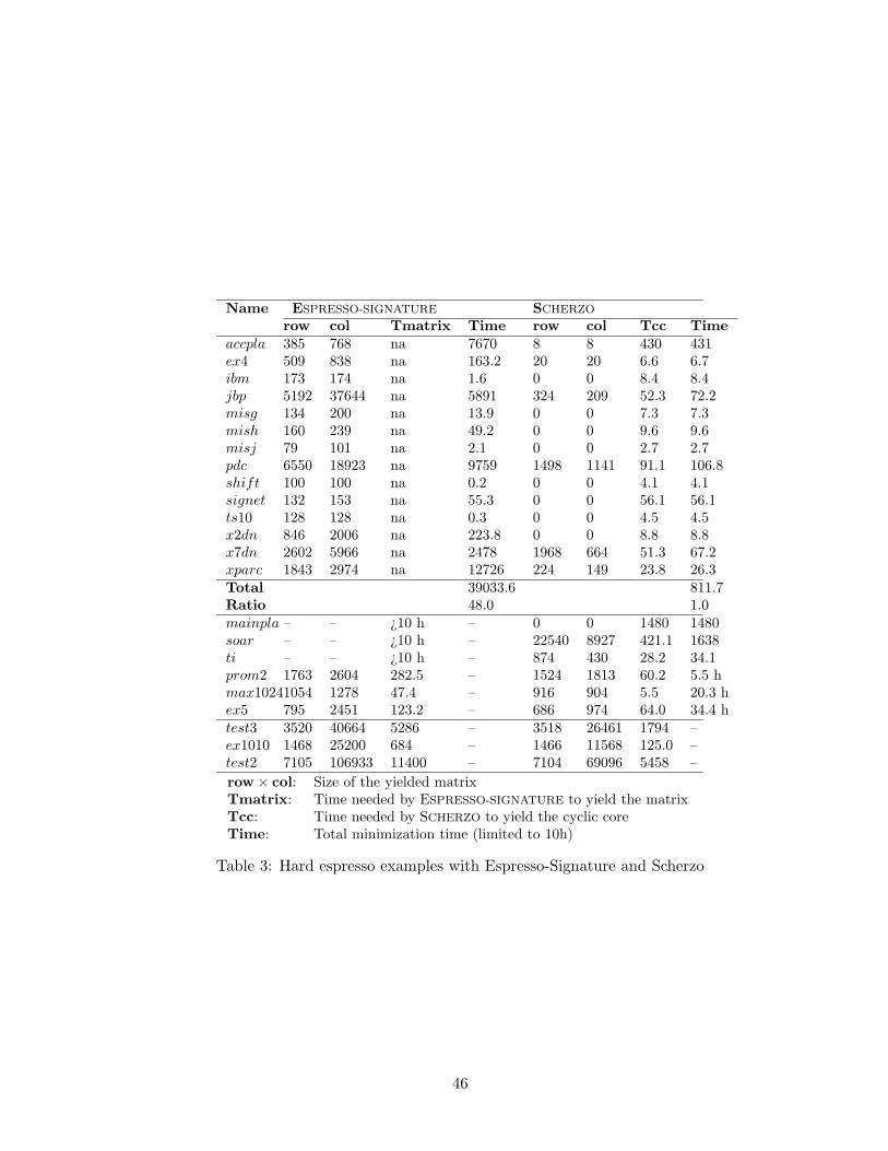
Name ESPRESSO-SIGNATURE SCHERZO

row col Tmatrix Time row col Tcc Timeaccpla 385 768 na 7670 8 8 430 431ex4 509 838 na 163.2 20 20 6.6 6.7ibm 173 174 na 1.6 0 0 8.4 8.4jbp 5192 37644 na 5891 324 209 52.3 72.2misg 134 200 na 13.9 0 0 7.3 7.3mish 160 239 na 49.2 0 0 9.6 9.6misj 79 101 na 2.1 0 0 2.7 2.7pdc 6550 18923 na 9759 1498 1141 91.1 106.8shift 100 100 na 0.2 0 0 4.1 4.1signet 132 153 na 55.3 0 0 56.1 56.1ts10 128 128 na 0.3 0 0 4.5 4.5x2dn 846 2006 na 223.8 0 0 8.8 8.8x7dn 2602 5966 na 2478 1968 664 51.3 67.2xparc 1843 2974 na 12726 224 149 23.8 26.3Total 39033.6 811.7Ratio 48.0 1.0mainpla – – ¿10 h – 0 0 1480 1480soar – – ¿10 h – 22540 8927 421.1 1638ti – – ¿10 h – 874 430 28.2 34.1prom2 1763 2604 282.5 – 1524 1813 60.2 5.5 hmax10241054 1278 47.4 – 916 904 5.5 20.3 hex5 795 2451 123.2 – 686 974 64.0 34.4 htest3 3520 40664 5286 – 3518 26461 1794 –ex1010 1468 25200 684 – 1466 11568 125.0 –test2 7105 106933 11400 – 7104 69096 5458 –

row × col: Size of the yielded matrixTmatrix: Time needed by ESPRESSO-SIGNATURE to yield the matrixTcc: Time needed by SCHERZO to yield the cyclic coreTime: Total minimization time (limited to 10h)

Table 3: Hard espresso examples with Espresso-Signature and Scherzo

46

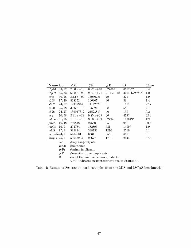
Name i/o #M #P #E B Timecbp16 33/17 7.30 e+10 6.87 e+10 327662 655287* 0.4cbp32 65/33 6.08 e+20 2.84 e+21 2.14 e+10 42949672823* 1.0cont 30/28 8.12 e+09 17060286 79 229 1.9s298 17/20 868352 106307 36 58 1.4s382 24/27 143293440 11142527 6 150* 27.7s420 35/18 3.86 e+10 125924 38 58 2.1s526 24/27 139917312 21523813 40 130 9.2seq 70/58 2.21 e+22 9.85 e+09 36 472* 62.4addsub 31/15 1.61 e+10 3.60 e+09 32794 163649* 171pitch 16/48 750848 27560 35 95 20.5rip08 16/9 294784 182893 631 1499* 1.9add8 17/9 589824 338732 1270 2519 0.1achil8n24/1 5764801 6561 6561 6561 0.1alupla 25/5 59653904 25677 1791 2144 37.5

i/o: #inputs/#outputs#M: #minterms#P: #prime implicants#E: #essential prime implicantsB: size of the minimal sum-of-products.

A “∗” indicates an improvement due to SCHERZO.

Table 4: Results of Scherzo on hard examples from the MIS and ISCAS benchmarks

47