Two Factors Full Factorial Design without Replications - Washington

21-1©2008 Raj JainCSE567MWashington University in St. Louis

Two Factors Two Factors Full Factorial Design Full Factorial Design without Replicationswithout Replications

Raj Jain Washington University in Saint Louis

Saint Louis, MO [email protected]

These slides are available on-line at:http://www.cse.wustl.edu/~jain/cse567-08/


OverviewOverview

! Computation of Effects! Estimating Experimental Errors! Allocation of Variation! ANOVA Table! Visual Tests! Confidence Intervals For Effects! Multiplicative Models! Missing Observations


Two Factors Full Factorial DesignTwo Factors Full Factorial Design! Used when there are two parameters that are carefully

controlled! Examples:

" To compare several processors using several workloads." To determining two configuration parameters, such as cache

and memory sizes! Assumes that the factors are categorical. For quantitative

factors, use a regression model.! A full factorial design with two factors A and B having a and b

levels requires ab experiments.! First consider the case where each experiment is conducted

only once.


ModelModel


Computation of EffectsComputation of Effects! Averaging the jth column produces:

! Since the last two terms are zero, we have:

! Similarly, averaging along rows produces:

! Averaging all observations produces

! Model parameters estimates are:

! Easily computed using a tabular arrangement.


Example 21.1: Cache ComparisonExample 21.1: Cache Comparison!


Example 21.1: Computation of EffectsExample 21.1: Computation of Effects

! An average workload on an average processor requires 72.2 ms of processor time.

! The time with two caches is 21.2 ms lower than that on an average processor

! The time with one cache is 20.2 ms lower than that on an average processor.

! The time without a cache is 41.4 ms higher than the average


Example 21.1 (Cont)Example 21.1 (Cont)! Two-cache - One-cache = 1 ms.! One-cache - No-cache = 41.4-20.2 or 21.2 ms.! The workloads also affect the processor time required. ! The ASM workload takes 0.5 ms less than the average.! TECO takes 8.8 ms higher than the average.


Estimating Experimental ErrorsEstimating Experimental Errors! Estimated response:

! Experimental error:

! Sum of squared errors (SSE):

! Example: The estimated processor time is:

! Error = Measured-Estimated = 54-50.5 = 3.5


Example 21.2: Error ComputationExample 21.2: Error Computation

The sum of squared errors is:


Example 21.2: Allocation of VariationExample 21.2: Allocation of Variation

! Squaring the model equation:

! High percent variation explained ⇒ Cache choice important in processor design.


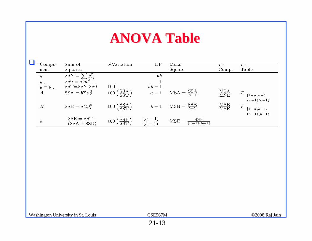
Analysis of VarianceAnalysis of Variance! Degrees of freedoms:

! Mean squares:

! Computed ratio > F[1- α;a-1,(a-1)(b-1)] ⇒ A is significant at level α.


ANOVA TableANOVA Table!


Example 21.3: Cache ComparisonExample 21.3: Cache Comparison

! Cache choice significant.! Workloads insignificant


Example 21.4: Visual TestsExample 21.4: Visual Tests


Confidence Intervals For EffectsConfidence Intervals For Effects

! For confidence intervals use t values at (a-1)(b-1) degrees of freedom


Example 21.5: Cache ComparisonExample 21.5: Cache Comparison! Standard deviation of errors:

! Standard deviation of the grand mean:

! Standard deviation of αj's:

! Standard deviation of βi's:


Example 21.5 (Cont)Example 21.5 (Cont)! Degrees of freedom for the errors are (a-1)(b-1)=8.

For 90% confidence interval, t[0.95;8]= 1.86.! Confidence interval for the grand mean:

! All three cache alternatives are significantly different from the average.


Example 21.5 (Cont)Example 21.5 (Cont)

! All workloads, except TECO, are similar to the average and hence to each other.


Example 21.5: CI for DifferencesExample 21.5: CI for Differences

! Two-cache and one-cache alternatives are both significantly better than a no cache alternative.

! There is no significant difference between two-cache and one-cache alternatives.


Case Study 21.1: Cache Design AlternativesCase Study 21.1: Cache Design Alternatives

! Multiprocess environment: Five jobs in parallel.ALL = ASM, TECO, SIEVE, DHRYSTONE, and SORT in parallel.

! Processor Time:


Case Study 21.1 on Cache Design (Cont)Case Study 21.1 on Cache Design (Cont)Confidence Intervals for Differences:

Conclusion: The two caches do not produce statistically better performance.


Multiplicative ModelsMultiplicative Models! Additive model:

! If factors multiply ⇒ Use multiplicative model! Example: processors and workloads

" Log of response follows an additive model! If the spread in the residuals increases with the mean response

⇒ Use transformation


Case Study 21.2: RISC architecturesCase Study 21.2: RISC architectures! Parallelism in time vs parallelism in space! Pipelining vs several units in parallel! Spectrum = HP9000/840 at 125 and 62.5 ns cycle! Scheme86 = Designed at MIT


Cache Study 21.2: Simulation ResultsCache Study 21.2: Simulation Results

! Additive model: ⇒ No significant difference! Easy to see that: Scheme86 = 2 or 3 × Spectrum125! Spectrum62.5 = 2 × Spectrum125! Execution Time = Processor Speed × Workload Size⇒ Multiplicative model.

! Observations skewed. ymax/ymin > 1000⇒ Adding not appropriate


Case Study 21.2: Multiplicative ModelCase Study 21.2: Multiplicative Model! Log Transformation:

! Effect of the processors is significant. ! The model explains 99.9% of variation as compared to 88% in

the additive model.


Case Study 21.2: Confidence IntervalsCase Study 21.2: Confidence Intervals

! Scheme86 and Spectrum62.5 are of comparable speed.! Spectrum125 is significantly slower than the other two

processors.! Scheme86's time is 0.4584 to 0.6115 times that of Spectrum125

and 0.7886 to 1.0520 times that of Spectrum62.5.! The time on Spectrum125 is 1.4894 to 1.9868 times that on

Spectrum62.5.


Cache Study 21.2: Visual TestsCache Study 21.2: Visual Tests


Case Study 21.2: ANOVACase Study 21.2: ANOVA

! Processors account for only 1% of the variation! Differences in the workloads account for 99%.⇒ Workloads widely different⇒ Use more workloads or cover a smaller range.


Case Study 21.3: ProcessorsCase Study 21.3: Processors


Case Study 21.3: Additive ModelCase Study 21.3: Additive Model

! Workloads explain 1.4% of the variation.! Only 6.7% of the variation is unexplained.


Case Study 21.3: Multiplicative ModelCase Study 21.3: Multiplicative Model

! Both models pass the visual tests equally well. ! It is more appropriate to say that processor B takes twice as

much time as processor A, than to say that processor B takes 50.7 ms more than processor A.


Case Study 21.3: IntelCase Study 21.3: Intel iAPXiAPX 432432!


Case Study 21.3: ANOVA with LogCase Study 21.3: ANOVA with Log

! Only 0.8% of variation is unexplained.Workloads explain a much larger percentage of variation than the systems⇒ the workload selection is poor.


Case Study 21.3: Confidence intervalsCase Study 21.3: Confidence intervals


Missing ObservationsMissing Observations! Recommended Method:

" Divide the sums by respective number of observations " Adjust the degrees of freedoms of sums of squares" Adjust formulas for standard deviations of effects

! Other Alternatives:" Replace the missing value by such that the residual for

the missing experiment is zero." Use y such that SSE is minimum.


Case Study 21.4: RISCCase Study 21.4: RISC--I Execution TimesI Execution Times

!


Case Study 21.5: Using Multiplicative ModelCase Study 21.5: Using Multiplicative Model

!


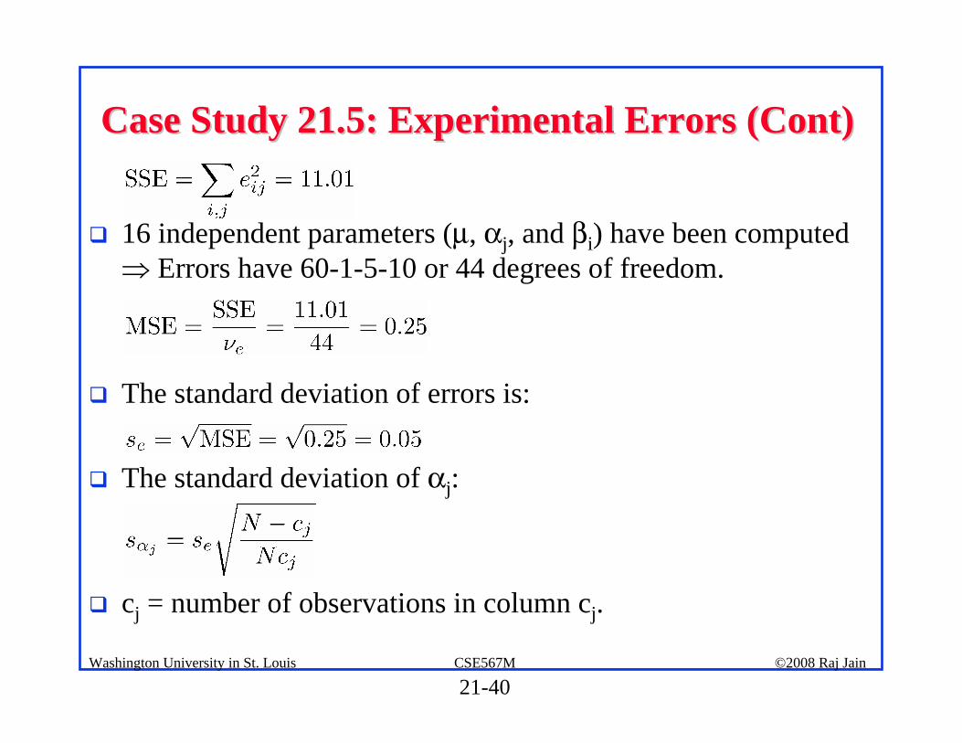
Case Study 21.5: Experimental ErrorsCase Study 21.5: Experimental Errors!


Case Study 21.5: Experimental Errors (Cont)Case Study 21.5: Experimental Errors (Cont)

! 16 independent parameters (μ, αj, and βi) have been computed ⇒ Errors have 60-1-5-10 or 44 degrees of freedom.

! The standard deviation of errors is:

! The standard deviation of αj:

! cj = number of observations in column cj.


Case Study 21.5 (Cont)Case Study 21.5 (Cont)! The standard deviation of the row effects:

ri=number of observations in the ith row.


Case Study 21.5: Case Study 21.5: CIsCIs for Processor Effectsfor Processor Effects


Case Study 21.5: Visual TestsCase Study 21.5: Visual Tests


Case Study 21.5: Analysis without 68000Case Study 21.5: Analysis without 68000


Case Study 21.5: RISCCase Study 21.5: RISC--I Code SizeI Code Size


Case Study 21.5: Confidence IntervalsCase Study 21.5: Confidence Intervals


SummarySummary

Two Factor Designs Without Replications! Model:

! Effects are computed so that:

! Effects:


Summary (Cont)Summary (Cont)! Allocation of variation: SSE can be calculated after computing

other terms below

! Mean squares:

! Analysis of variance:


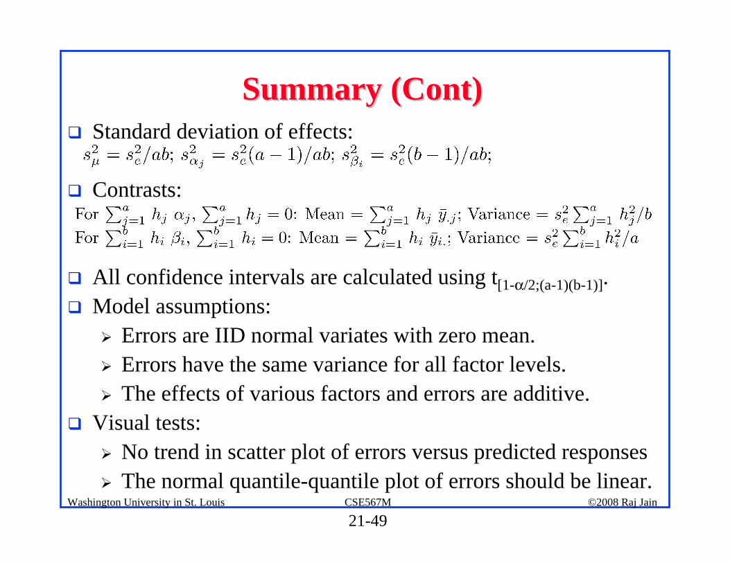
Summary (Cont)Summary (Cont)! Standard deviation of effects:

! Contrasts:

! All confidence intervals are calculated using t[1-α/2;(a-1)(b-1)].! Model assumptions:

" Errors are IID normal variates with zero mean." Errors have the same variance for all factor levels." The effects of various factors and errors are additive.

! Visual tests:" No trend in scatter plot of errors versus predicted responses" The normal quantile-quantile plot of errors should be linear.


Exercise 21.1Exercise 21.1Analyze the data of Case study 21.2 using an additive model.! Plot residuals as a function of predicted response.! Also, plot a normal quantile-quantile plot for the residuals.! Determine 90% confidence intervals for the paired differences. ! Are the processors significantly different?! Discuss what indicators in the data, analysis, or plot would

suggest that this is not a good model.


Exercise 21.2Exercise 21.2Analyze the data of Table 21.18 using a multiplicative model and

verify your analysis with the results presented in Table 21.19.


Exercise 21.3Exercise 21.3Analyze the code size data of Table 21.23. Ignore the second

column corresponding to 68000 for this exercise.Answer the following:a. What percentage of variation is explained by the

processor?b. What percentage of variation can be attributed to the

workload?c. Is there a significant (at 90% confidence) difference

between any two processors?


Exercise 21.4Exercise 21.4Repeat Exercise 21.3 with the 68000 column included.


HomeworkHomework! Submit answer to Exercise 21.1

Two Factors Full Factorial Design without Replications - Washington

Documents

Transcript of Two Factors Full Factorial Design without Replications - Washington