Two Dimensional flow of Shear Thinning Fluid around a ...

Two Dimensional flow of Shear

Thinning Fluid

around a Circular Cylinder

A Thesis Submitted in Partial Fulfilment of

the Requirements for the degree of

“BACHELOR OF TECHNOLOGY IN CHEMICAL ENGINEERING”

By:

Pritish Kumar Choudhury,

111CH0618,

Department of Chemical Engineering,

National Institute of Technology,

Rourkela.

Under the Guidance of

Prof. Akhilesh Sahu,


National Institute of Technology, Rourkela.

May 2015

This is to certify that the thesis under the title “

Fluid around a Circular Cylinder

(111CH0618), in partial fulfilments for the requirements of the award of Bachelor of

Technology Degree in Chemical Engineering at National Institute of Technology, Rourkela

has been carried out under my supervision and guidance.

Date-

Place-

i

Certificate

that the thesis under the title “Two Dimensional flow of Shear Thinning

ircular Cylinder” presented by Pritish Kumar Choudhury

in partial fulfilments for the requirements of the award of Bachelor of


has been carried out under my supervision and guidance.




Two Dimensional flow of Shear Thinning

Pritish Kumar Choudhury

in partial fulfilments for the requirements of the award of Bachelor of





Rourkela-769008

.

ii

Acknowledgement

I would like to express my overwhelming gratitude to Dr. Akhilesh Sahu, my ‘Project Guide

and Thesis Supervisor’ for his enormous help and deep encouragement throughout the

process starting from the help in my B.Tech Project completion to the Thesis work. He has

been a constant guide and support during any sort of problem during the project. He has

provided me with tremendous knowledge on the field of “Computational Fluid Dynamics”.

I would like to express my gratitude to Dr. P Rath, ‘Head of the Department’ and Department

of Chemical Engineering for allowing me to undertake this project. I had a keen interest for

working in the field of CFD and I am extremely grateful for granting me the opportunity to

do so.

I would like to thank Dr. P Chowdhary, ‘Faculty Advisor of Class-2015’ for being there with

me at all times of problems. He is great person to talk to during any type of academic and

non-academic problems. He has always helped me in all possible ways and encouraged me

with his endeavours.

I would like to thank my project mates Amogh, Bishmaya and Eugine and all of my friends

for a great company to work with. They have always made the work interesting and the

project time to be a fun. I would like to thank Trupti Ranjan Behera and Akhilesh Khappre

for constant help in ANSYS software and simulations.

I would like to express my heartfelt gratitude to my parents and my family members those

who have supported me emotionally and been a constant support for me throughout my life. I

would also thank the Almighty for this wonderful life.

Pritish Kumar Choudhury,

111CH0618,


NIT Rourkela.

iii

Abstract

The Present Research work is done on the domain of Computational Fluid Dynamics (CFD).

The entire work is done in the FLUENT component of ANSYS. The study of flow property

has been divided into three phases. The first phase was getting familiar with the software

ANSYS-FLUENT and learning its application and utility on the problem of a lid-driven

square cavity. The work was done for both Newtonian (n=1) and shear-thinning Non-

Newtonian fluid (n=0.5) fluid flow for a set of Reynolds numbers (100<Re<10,000). The

flow was incompressible and in Laminar Regime.

The next phase of the work was to study the problem in hand, i.e., flow past a circular

cylinder for a square domain in a steady state condition to determine the value of drag-

coefficient. The flow was taken to be incompressible and in the laminar region. Here the fluid

considered was both Newtonian (n=1) and Non-Newtonian (n=0.6 and n=0.8). The values of

the drag-coefficient obtained were validated from the literature. Then the final task was to

test the laminar incompressible fluid flow around circular cylinder for a unsteady state

condition and a bit more complicated geometry, i.e., an interim between square and circular

geometry for a Newtonian and a Non-Newtonian fluid (n=0.5). The study was done by

varying the Reynolds number (60<Re<100). The values of average drag-coefficient, Root

Mean Square value of lift-coefficient and Strouhal Number was plotted versus the considered

Reynolds Number range. The flow pattern in an unsteady laminar incompressible flow was

also studied.

Keywords: Non-Newtonian, Drag Coefficient, Lift Coefficient, Reynolds No, Strouhal No

iv

Contents

Certificate i Acknowledgement ii Abstract iii

Chapter No

Topics Page No

Nomenclature of Symbols 1 Index of Figures and Tables 2 1. Introduction 3 2. Literature Review 4 3. Problem Statement 6 4. Results and Discussions 8 4.1 Lid Driven Cavity 9

4.2 Steady flow past a circular cylinder 15 4.3 Unsteady flow past a circular cylinder 17 4.4 Determination of Point of Unsteady 25 5. Conclusion 27 6. Bibliography 28

1

Nomenclature of Symbols:

Symbols Relevance Symbol Relevance D Diameter of the Cylinder (m) ε Strain Tensor rate CD Drag Coefficient n Power Law Index CDP Pressure component of Drag

coefficient CDF Friction Component of Drag

coefficient I2 Second Invariant of deformation

tensor rate ∇ �

�� +

�

��

CP Pressure Coefficient f Body Force FD Drag Force (N) Ux x-component of Velocity (m s-1) FDF Frictional Drag Force (N) Uy y-component of Velocity (m s-1) FDP Pressure Drag Force (N) σ Stress Tensor H Height of the domain Geometry (m) u Velocity of the fluid (m s-1) η Viscosity (kgm-1s-1) � Stream Function � Density (kg m-3) D∞ Length of Domain Geometry (m) Y Ordinate of Mesh Re Reynolds No

Rec Critical Reynolds No Stc Critical Strouhal No

k Power Law Consistency Index f Vortex Shedding Frequency (s-1) P Pressure (Pa) Δ Difference/gradient

2

Index of Figures and Tables

For Figures:

Figure No.

Caption Page No.

Fig.3.1 Unsteady Flow around circular cylinder Geometry 6 Fig.4.1 Lid Driven Square Cavity Geometry 9 Fig.4.2 Stream Function for 100<Re<10,00 in Square Cavity Newtonian Flow 10 Fig.4.3 HCL and VCL Velocity for Re=100 and Re=10,00 for Newtonian fluid 11 Fig.4.4 Validation of HCL and VCL for Re=100 &400 for Newtonian 12 Fig.4.5 Stream Function for n=0.5 & 0.75 in Square Cavity non-Newtonian Flow 13 Fig.4.6 Validation of HCL and VCL for Re=100 & 400 for non-Newtonian 14 Fig.4.7 Steady Flow around circular cylinder Geometry 16 Fig.4.8 Unsteady Flow around circular cylinder Geometry 18 Fig.4.9 Drag and lift vs. Time plot for different Re, unsteady state Newtonian 19 Fig.4.10 Streamlines and Velocity Mag. Re 70 & 100,unsteady state Newtonian 20 Fig.4.11 Post Processing for Newtonian flow and unsteady state 21 Fig.4.12 Drag and lift vs. Time plot for different Re, unsteady non-Newtonian 22 Fig.4.13 Streamlines & Velocity Mag. Re 70 & 100,unsteady state non- Newtonian 23 Fig.4.14 Post Processing for non-Newtonian flow and unsteady state 24 Fig.4.15 Determination of Point of Unsteady for Newtonian Flow by Drag vs. Time 25 Fig.4.16 Determination of Point of Unsteady for Newtonian Flow by Velocity Mag. 26

For Tables:

Table No. Caption Page No.

Table.4.1 Validation of Drag values for Reynolds no=20 for n=0.6, 0.8 & 1.0 16 Table.4.2 Average Drag, RMS Value of Lift and Strouhal No vs. Reynolds No for

Newtonian flow at unsteady condition 21

Table.4.3 Average Drag, RMS Value of Lift and Strouhal No vs. Reynolds No for Non-Newtonian flow at unsteady condition

24

3

1) Introduction

The occasional vortex shedding among the bluff bodies in presence of uniform flow has been

a fascination for researchers and scholars of the likes of Leonardo Da Vinci. The origin of the

flow can be considered as the instabilities and disruptions in the channel of flow and further it

is largely dependent on the fluid’s Reynolds Number. To engineers the integral parameters

that find keen interest are not only the steam function and vector plot as well as an extensive

study on average drag, RMS value of lift as well as the Strouhal number. Majority of the

engineering problems needs the investigation of flows of both nature, i.e., Newtonian (n=1)

and non-Newtonian (Shear-Thinning n<1 and Shear-Thickening n>1). The viscous flow by

Non-Newtonian fluids and the categories of related constitutive equations they provide has

numerous utility in petroleum, food industry, lubricants and blood flow. The approach of

computational fluid dynamics (CFD) to a non-Newtonian problem is usually more

complicated than a Newtonian one as the complexity is increased by the Navier-Stokes

constitutive equation of diffusion terms.

We have numerous equations and numerical models at our disposal for simulating the viscous

fluid flow, and out of which the most common model is the Power-Law Model. The finite

element method (FEM) has been employed in several studies for investigation of the fully

developed laminar flow of a power-law non-Newtonian fluid in a rectangular duct. While the

finite volume (FV) method is applied mostly in visco-elastic fluid flows [24]. There are

numerous drawbacks in the FV methods, i.e., induction of artificial diffusion by low order

interpolation of the convection term of the Navier–Stokes equations. For overcoming these

specified effects, interpolation schemes of higher order have been developed. Out of which a

very popular scheme is the QUICK (Quadratic Upwind Interpolation for Convective

Kinematics) scheme, which is 3rd order accurate. Thus, it has higher order of accuracy than

low order equations.

The bluff-body flows are under a lot of research as it has a huge application in energy

conservation. For understanding this kind of flow the simplest obstacle which is a circular

cylinder is taken. One important thing that must be kept in mind is that in circular cylinder

there are no distinct separation points of contact unlike that in square cylinder which have at

its corners. During extensive study in literature, there exists humongous work on Newtonian

fluid flow at a high value of Reynolds Number. But, very scarce is done at a low value of

Reynolds no for Non-Newtonian flow.

4

2) Literature Review

The flow of fluids past a circular cylinder is of immense importance in the field of fluid

mechanics and thus has received tremendous attention in the literature and study. Thus, in the

past years the flow over circular cylinder has been a constant source of attraction from

numerical, experimental as well as analytical prospective, ([1]–[5]). There are numerous

experimental studies on vortex shedding flows by Bearman [6], but knowledge in full details

for unsteady flow is absent due to the considerable effort is needed to understand the

unsteady flow. But, there lies an exception; it is the work of Cantwell and Coles [7]. They

studied the turbulent flow past a circular cylinder Reynolds number value as high as 140,000

by the help of a flying hotwire. They were successful separating the periodic and turbulent

fluctuations and also did present phase-averaged values for various phases during one cycle

for the velocity components.

Vortex-shedding flow past cylindrical structures has brought keen interests among the

numerical analysts. Son and Hanratty [8] have published numerical solutions of the unsteady

two-dimensional Navier-Stokes equations for the flow around a circular cylinder for low

values of Reynolds number; Re < 500. Majority of earlier calculation had a drawback of

absence of super computers to calculate for them and even calculation shad to be made at

personal level. Nowadays there is a change in the scenario. Braza et al. [9] utilised a FV

method for understanding the vortex shedding past circular cylinders for Re<1000, and

Lecointe and Piquet [10] calculated the flow around the circular cylinder for both steady as

well as transient state by finite difference method. Lecointe and piquet did apply vorticity and

stream function concept which that their own shortcomings that they could not be applied to

three-dimensional flow.

Only for Newtonian fluids, Sharma and Eswaran [11, 12] have reported new numerical

results on force (drag and lift) coefficients and Strouhal number for the values of Reynolds

number Re <= 160. For Newtonian fluids, typically for an unconfined uniform flow oriented

transverse to the long axis of the cylinder, the flow remains attached to the surface up to

about Re = 1–2 beyond which it separates and two-symmetric vortices appear in the rear

which remain attached to the surface of the obstacle, but grow in length along the direction of

flow up to about Re = 40–45[34]. Under these conditions, the flow field near the obstacle is

time-independent and two-dimensional. With further increase in the value of the Reynolds

number, the wake becomes asymmetric and the flow transits to the laminar vortex shedding

regime which is characterized in terms of alternate shedding of vortices from the upper half

and lower half of the cylinder. This makes the flow near the cylinder periodic in time, but it is

still two-dimensional [34]. Naturally, the changes in the detailed kinematics of the flow also

manifest at the macroscopic level, because the global parameters like drag coefficient scale

differently with Reynolds number in different regimes. All in all, an adequate body of

information is thus available on the momentum transfer coefficients for a square cylinder

immersed in Newtonian fluids up to about Re < 160 which is almost the limit of the laminar

vortex shedding regime [34]. The effects of confinement and of buoyancy on momentum

5

transfer coefficients have also been studied fairly widely [13-16]. The influence of confining

walls on momentum transfer characteristics are modulated by the value of the Reynolds

number.

Tanner [17] demonstrated that there is absence of Stokes Paradox as the Reynolds Number

approaches to zero in the case of shear thinning fluids. This is due to the fact that the

effective shear rate in the fluid falls rapidly as we move away from the cylinder. For shear

thinning fluids, this implies a progressive increase in the viscous forces whereas the viscous

forces diminish for a shear thickening fluid. Subsequently a similar inference was also drawn

by others [18]. Tanner [17] was able to obtain approximate analytical results for the creeping

flow of power law fluids past a circular cylinder for shear thinning fluids. He also

supplemented these results with numerical predictions in the range n = 0.4 to 0.9; the

correspondence was found to be reasonable. Subsequently, these results have been extended

to even smaller values of the power law index up to n = 0:2 [19]. However, all these results

only relate to the zero Reynolds number and shear thinning fluid behaviour. D’Alessio and

Pascal [20] numerically investigated the steady power-law flow around a cylinder at

Reynolds numbers Re = 5, 20 and 40 using a first-order accurate difference method for a

fixed blockage ratio 0.037. They investigated the dependence of critical Reynolds number,

wake length, separation angle and drag coefficient on the power-law index. They reported

that as the value of the Reynolds number was progressively increased there was a decreasing

degree of convergence which restricted the range of power law indices for which a numerical

solution was possible. It is also important to determine the dependence of the aforementioned

parameters on the distance from the cylinder surface to the external numerical boundary (the

blockage effect), since an increase in this distance approximates the conditions of flow in an

infinite extent of fluid or, equivalently, decreases the wall effects. Although the effect of

blockage on flow parameters and/or stream line patterns is well documented for Newtonian

fluids ([21]–[23]) as well as for non–Newtonian viscoelastic fluids, both numerically and

experimentally in the creeping flow region ([24]–[25]), a corresponding investigation for

non–Newtonian visco-inelastic power law fluids is lacking.

6

3) Problem Statement

Let us consider the 2-D flow of an incompressible power-law liquid with a uniform velocity

of a value U∞ flowing across a long circular cylinder of diameter D. The simulation of

unconfined flow condition is done by considering the circular cylinder of diameter D placed

in the geometry given (Fig.3.1). The diameter of the outer circular boundary D∞ is taken to be

sufficiently large to minimize the boundary effects. The continuity and momentum equations

for this flow are written as:

Continuity equation:

∇.u=0 (Equation 3.1)

Momentum Equation:

� (��

��+ �. ��) - ∇. σ =0 (Equation 3.2)

Where�, u, and σ are the density, velocity (Ux and Uy) and the stress tensor, respectively.

The equation of state for the given power-law fluids is given by:

σ =2 η ε (u) (Equation 3.3)

Where ε (u) is the vector components of the strain tensor rate that is related to velocity field

in Cartesian coordinate system, and is given by

ε (u) = ½ {(∇.u) + (∇.u) T} (Equation 3.4)

The viscosity, η, is given by

η= (I2/2) (n-1)/2 (Equation 3.5)

Where n is the power-law index (n< 1 for shear-thinning; n=1 for Newtonian; and n>1 for

shear-thickening fluids) and I2 is the second invariant of the rate of strain tensor.

Figure-3.1

7

The boundary conditions for this flow may be written as follows:

• At the inlet boundary: There is a fluid flow of condition

Ux = U∞ and Uy = 0.

• On the circular cylinder: The condition considered is no-slip flow:

Ux = 0 and Uy = 0.

• At the exit boundary:

Outflow condition which means zero diffusion flux (i.e., �∅

�� = 0, where ∅ is a scalar variable),

were used. Here ∅ can be anything Pressure, Temperature, Velocity components etc.

The symmetry in the top and bottom wall needs to be broken in order to obtain unsteady state

profile. Hence, the symmetry was broken by the introduction of custom field function:��|�|

��

The numerical solution of Equations along with the above-noted boundary conditions

provide us with the velocity and pressure fields and which are used for deduction of the

global characteristics like drag and lift coefficients as well as the Strouhal number. There are

two important parameters that govern the type of flow in the cylinder, i.e., Reynolds number

and power-law index (n). In the unsteady flow regime, there is an additional dimensionless

group of Strouhal number. Now some definitions are as:

Reynolds number: The Reynolds number (Re) for power-law fluids is defined as

follows:

Reynolds number: Re = ��

�

Critical Reynolds numbers: The definition of critical Reynolds numbers (Rec and Rec)

is as the value of Reynolds number where there is emergence of wake (Rec) and the other

critical Reynolds number (Rec) refers to the point of shift from steady to unsteady regime.

Drag and lift coefficients: The mathematical definition of drag and lift coefficients goes:

CD=��

��

=CDP+CDF

(Here FD=Drag Force)

CL=��

��

(Here FL=Lift Force)

CDP and CDF are pressure and friction drag coefficients, respectively.

Strouhal number: The Strouhal number (St) is the dimensionless frequency of vortex

shedding,

St = ��

��where ‘f’ is the vortex shedding frequency. The value of the Strouhal number at

the critical Reynolds number is termed critical Strouhal number (Stc). Obviously, the

values of both lift coefficient and the Strouhal number will be zero for the steady flow

regime conditions. Here, the value of vortex shedding frequency was determined from the

lift vs. time plot.

8

4) Results and Discussions

This part is of utmost importance. Here all the simulation procedure is present along with the

concept behind the simulation. The content of the part is divided into 3 sub-units:

1. Lid-Driven Square Cavity Problem.

2. Steady state flow around Circular Cylinder Problem.

3. Unsteady State flow around a Circular Cylinder Problem.

All of the mentioned topics are covered for both Newtonian (n=1) type of fluids as well as

Shear Thinning non-Newtonian (n<1) type of fluids.

Various Plots and tables are generated in each sub-unit to support the argument presented

after this section. Also various Stream Function, Vector Plot and Velocity Magnitude Plot are

also presented in order to understand the flow nature in the given domain.

9

4.1 LID DRIVEN SQUARE CAVITY

The laminar incompressible flow in a square cavity whose top wall moves with a uniform

velocity in its own plane has served over and over again as a model problem for testing and

evaluating numerical techniques, in spite of the singularities at two of its corners. For

moderately high values of the Reynolds number Re, published results are available for this

flow problem from a number of sources [26-28], using a variety of solution procedures,

including an attempt to extract analytically the corner singularities from the dependent

variables of the problem [29]. Some results are also available for high Reynolds No [30], but

the accuracy of most of these high-Re solutions has generally been viewed with some

scepticism because of the size of the computational mesh employed and the difficulties

experienced with convergence of conventional iterative numerical methods for these cases.

Possible exceptions to these may be the results obtained by Benjamin and Denny (41 for Re =

10,000 using a non-uniform 151 X 151 grid such that Δx = Δy= l/400 near the walls and those

of Agarwal [31] for Re = 7500 using a uniform 121 x 121 grid together with a higher order

accurate upwind scheme.

The present study aims at studying the fluid flow in the lid-driven square cavity for a set of

Reynolds Number 100<Re<10,000 for the Newtonian fluids [Fig 3-8].The Stream functions

at all of the considered Reynolds number are found out. And for the validation purpose Ghia

et al. [32] was considered (Fig.4.4). Here the y-component of the velocity at horizontal

Centre line and x-component at Vertical Centre Line is found out (Fig.4.3) Now, for the non-

Newtonian case, the value of Reynolds no was fixed at Re=100 and the values of Power Law

Index is varied (n=0.5 and n=0.75). Again the vector plot (Fig.4.5) is found for understanding

the flow pattern. In this case, again the validation is done by comparing the normal

component of Centre Line velocities with Neofytou [33] Data (Fig.4.6).

The Geometry (Fig-2) is a simple square one with top lid being a moving wall with a velocity

that can be evaluated from the expression of Reynolds No given the material under use being

water. Here the mesh is normal square mesh of dimension 151 x 51 found from [32]. With a

specified residual in continuity and both the momentum transport equation being < 10-6 the

converged solution is plotted.

Fig-4.1 Schematics for Lid-Driven Cavity

10

1. Stream Function Plot for various Reynolds Number for Newtonian fluid:

The above below are for the instantaneous Stream lines contours for different values of

Reynolds Number are shown. These plots demonstrate the nature of fluid flow in the

geometry. The variation is considered from Reynolds no 100< Re < 10,000.

Fig.4.2 (a) Stream lines for Re=100

Fig.4.2 (b) Stream lines for Re=400

Fig.4.2 (c) Stream lines for Re=3200

Fig.4.2 (d) Stream lines for Re=10,000

At lower value of Reynolds No say at Re=100, the position of wake is somewhat at the centre

with respect to the horizontal plane. But, as we have increased the Reynolds No the wake

portion is shifted towards the right hand portion of the cavity. This is because at higher

Reynolds No the velocity is quite high which affects the wake in the given manner.

11

2. Horizontal Centre line and Vertical Centre Line Velocity for various Reynolds No

for Newtonian Fluid:

The first two figures demonstrate the Vertical component of Horizontal Centre Line and

the mater two figures demonstrate the Horizontal Component of Vertical Centre Line.

The variation is considered for Reynolds No=100 and 400.

Fig.4.3 (a) Horizontal Centre Line Re=100

Fig.4.3 (b) Horizontal Centre Line Re- 400)

Fig.4.3 (c) Vertical Centre Line Re=100

Fig.4.3 (d) Vertical Centre Line Re=400

The first half of HCL has the flow in upward direction and as we move from the wall

towards the centre the velocity initially is zero due to no slip condition and then the

velocity increases to a maximum and further drops to zero due to its distance from the

walls and the effects were not felt at the centre and further moving away from the centre

in the right half the velocity/ flow direction is downward direction which can be seen in

the plot.

The bottom portion of VCL practically has zero velocity at the walls due to the no slip

boundary condition has zero velocity at the proximity of bottom wall. The top wall

velocity is fixed the lid velocity which can be seen from the plot.

3. Validation from literature with plots

This section of the discussion is dedicated towards the validation of the results obtained from

Ghia et al. Work [36]. The main purpose of validation is to demonstrate the consistency of

model.


Fig.4.4 (b) Vertical Centre Line Re=100

The Value of x-component of Velocity at Vertical Centre line and y

at Horizontal Centre Line is plotted for Reynolds No 100 and 400 values. These results

obtained are quite encouraging.

with that in the literature.



VCL practically has zero velocity at the walls due to the no slip

has zero velocity at the proximity of bottom wall. The top wall

velocity is fixed the lid velocity which can be seen from the plot.

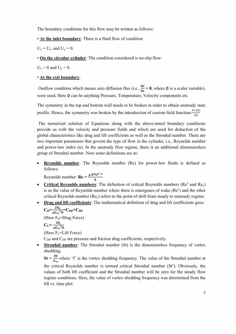
Validation from literature with plots from Ghia et al. for Newtonian flow:



Horizontal Centre Line Re=100

l Centre Line Re=100

Fig.4.4 (c) Horizontal Centre Line


component of Velocity at Vertical Centre line and y-component of Velocity


encouraging. This means that the setup we have used is in qui

12



VCL practically has zero velocity at the walls due to the no slip

has zero velocity at the proximity of bottom wall. The top wall

from Ghia et al. for Newtonian flow:



Horizontal Centre Line Re=400

Centre Line Re=100

component of Velocity


This means that the setup we have used is in quite accordance

13

4. Vector Plot for Reynolds No 100 and different values of Power Law Index for a non-

Newtonian fluid flow:

The below plots are the vector plots for the non-Newtonian case. This has a lot of

application that the arrows in the vector plot show the magnitude with the length and the

direction using arrows. The variation is for n=0.5 and n=0.75

Fig.4.5 (a) Re=100 and n=0.5

Fig.4.5 (b) Re=100 and n=0.75

However, for non-Newtonian flow the nature of fluid flow inside the cavity was

demonstrated by the vector plot. This was done to show the onset of formation of wakes at

the bottom corners of the cavity. The plot given doesn’t clearly display the wake but upon

further zooming of the image at the bottom corners the formation and direction of wakes are

clearly visible.

14

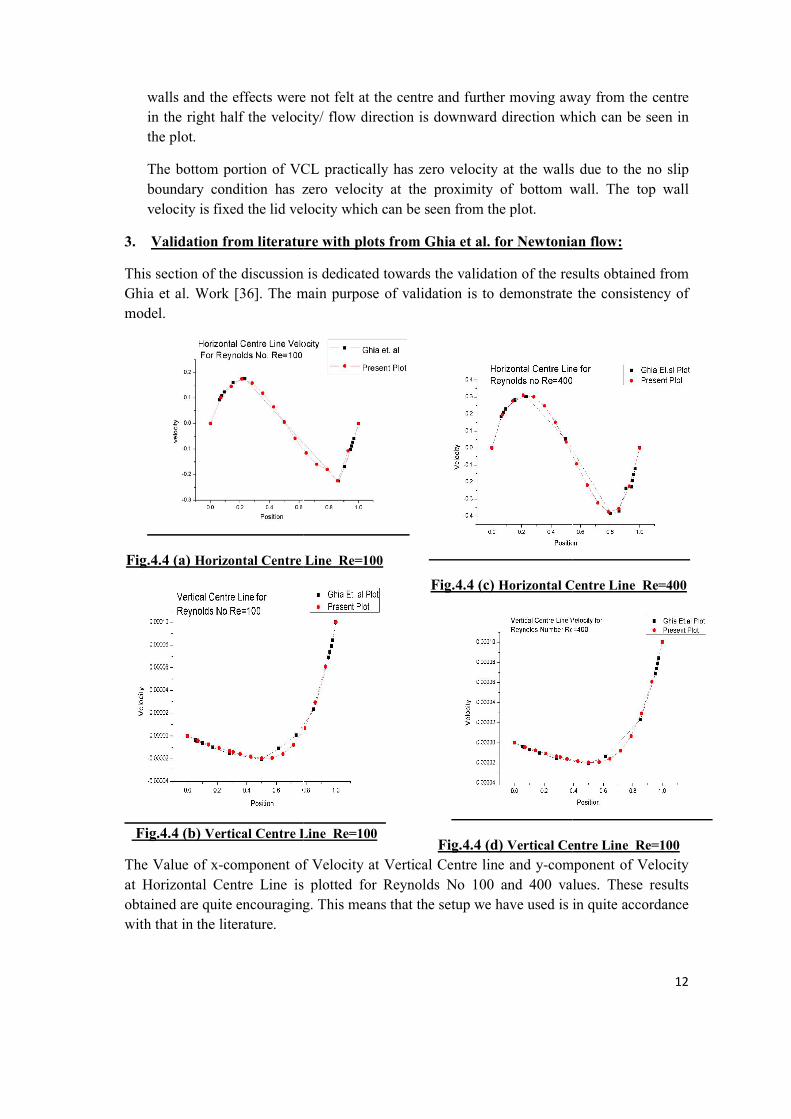
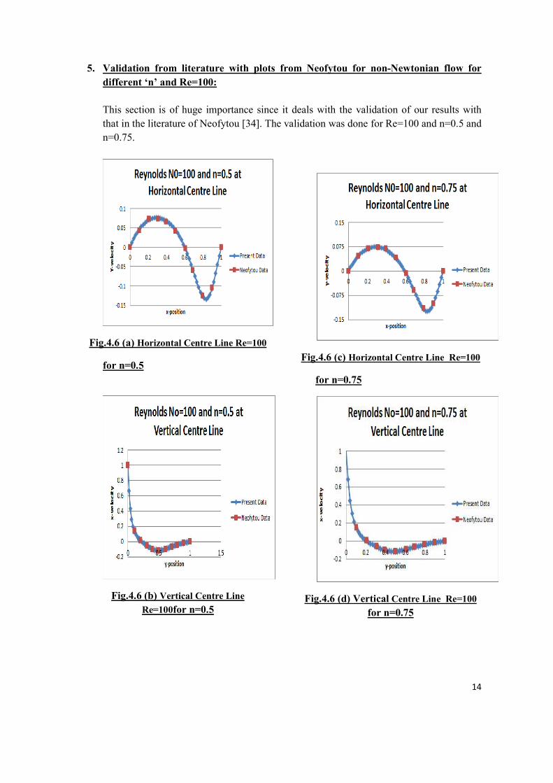
5. Validation from literature with plots from Neofytou for non-Newtonian flow for

different ‘n’ and Re=100:

This section is of huge importance since it deals with the validation of our results with

that in the literature of Neofytou [34]. The validation was done for Re=100 and n=0.5 and

n=0.75.


for n=0.5

Fig.4.6 (b) Vertical Centre Line

Re=100for n=0.5

Fig.4.6 (c) Horizontal Centre Line Re=100

for n=0.75


for n=0.75

15

4.2 STEADY STATE FLOW PAST A CIRCULAR CYLINDER

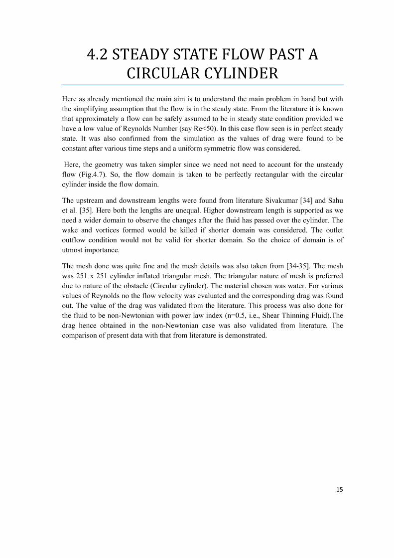
Here as already mentioned the main aim is to understand the main problem in hand but with

the simplifying assumption that the flow is in the steady state. From the literature it is known

that approximately a flow can be safely assumed to be in steady state condition provided we

have a low value of Reynolds Number (say Re<50). In this case flow seen is in perfect steady

state. It was also confirmed from the simulation as the values of drag were found to be

constant after various time steps and a uniform symmetric flow was considered.

Here, the geometry was taken simpler since we need not need to account for the unsteady

flow (Fig.4.7). So, the flow domain is taken to be perfectly rectangular with the circular

cylinder inside the flow domain.

The upstream and downstream lengths were found from literature Sivakumar [34] and Sahu

et al. [35]. Here both the lengths are unequal. Higher downstream length is supported as we

need a wider domain to observe the changes after the fluid has passed over the cylinder. The

wake and vortices formed would be killed if shorter domain was considered. The outlet

outflow condition would not be valid for shorter domain. So the choice of domain is of

utmost importance.

The mesh done was quite fine and the mesh details was also taken from [34-35]. The mesh

was 251 x 251 cylinder inflated triangular mesh. The triangular nature of mesh is preferred

due to nature of the obstacle (Circular cylinder). The material chosen was water. For various

values of Reynolds no the flow velocity was evaluated and the corresponding drag was found

out. The value of the drag was validated from the literature. This process was also done for

the fluid to be non-Newtonian with power law index (n=0.5, i.e., Shear Thinning Fluid).The

drag hence obtained in the non-Newtonian case was also validated from literature. The

comparison of present data with that from literature is demonstrated.

16

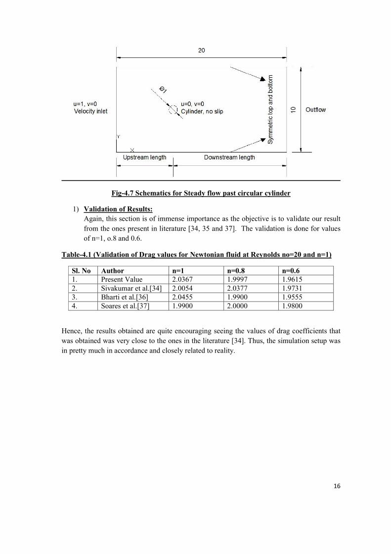
Fig-4.7 Schematics for Steady flow past circular cylinder

1) Validation of Results:

Again, this section is of immense importance as the objective is to validate our result

from the ones present in literature [34, 35 and 37]. The validation is done for values

of n=1, o.8 and 0.6.

Table-4.1 (Validation of Drag values for Newtonian fluid at Reynolds no=20 and n=1)

Sl. No Author n=1 n=0.8 n=0.6 1. Present Value 2.0367 1.9997 1.9615 2. Sivakumar et al.[34] 2.0054 2.0377 1.9731 3. Bharti et al.[36] 2.0455 1.9900 1.9555 4. Soares et al.[37] 1.9900 2.0000 1.9800

Hence, the results obtained are quite encouraging seeing the values of drag coefficients that

was obtained was very close to the ones in the literature [34]. Thus, the simulation setup was

in pretty much in accordance and closely related to reality.

17

4.3 UNSTEADY STATE FLOW PAST A CIRCULAR CYLINDER

The present numerical study has been carried out using FLUENT (version 15). The

unstructured ‘quadrilateral’ cells of non-uniform spacing were generated using Geometry

and Meshing Section of ANSYS. The grid near the surface of the cylinder was sufficiently

fine to resolve the flow within the boundary layer. For further refining of the grid in was

used. Furthermore, the unsteady laminar segregated solver was used with second order

upwinding scheme for the convective terms in the momentum equation. The semi-implicit

method for the pressure linked equations (SIMPLE) scheme was used for pressure–velocity

coupling and non-Newtonian power-law model was used for viscosity. In the present study, a

convergence criterion of 1 × 10−10 was used for the residuals of all variables. The iterations

were stopped when the oscillations of the lift coefficients either reached a periodic steady

state or when these die out completely.

It is the extension of the phase-2; here we incorporate the unsteady factor, i.e., the time

dependency of drag. The important parameters are Vortex Shedding Frequency, RMS value

of lift and the Strouhal no. All of the specified parameters are a function of Reynolds No.

Here the geometry is bot different than used earlier. The input wall is circular in nature. The

geometry is shown in Fig-4.8. After inputting the upstream and downstream lengths, next

comes the turn of meshing. As discussed already, for a circular cylinder a triangular mesh is

needed [34]. The dimension of mesh is taken to be 251 x 251 [36]. The inlet, top and bottom

wall is mentioned as velocity inlet whereas the cylinder is taken to be no slip wall. The outlet

is maintained as Pressure-Outflow or Outlet Condition. There exists a symmetric condition

at top and bottom wall. It needs to be broken in order to obtain time-dependent Drag. This is

done by incorporating custom field function after standard initialisation is done:

Custom Field Function: ��|�|

�� where Y is the mesh coordinate along y-axis. So this provides a

value ‘1’ in the top half and a ‘0’ value in the bottom half. Hence, the symmetry is broken.

Here for Newtonian flow, the velocity is taken to be 1m/s, Viscosity of the fluid is taken to be

0.01Nm-1s-1. For different values of Reynolds No the corresponding Density is fixed while

keeping others constant. Now for different sets of Reynolds no different values of Average

drag, RMS value of Lift and Strouhal no is evaluated. The plots of Drag and lift for sets of

Reynolds no is shown (Fig.4.9). After calculation of the values the results are tabulated

(Table.4.2). The Stream Function and Velocity Magnitude are in (Fig.4.10). Here time step is

0.2 sec with 10000 time steps in total.

Now for post processing the plots of average Drag, RMS value of Lift and Strouhal no vs.

Reynolds No is drawn (Fig.4.11).

18

Now for the case of non-Newtonian fluid, we again vary the Reynolds no to see its effect on

Average drag, RMS value of Lift and Strouhal No. But unlike the previous case we take the

velocity to be 0.5m/s. Now the power law index was considered to be n=0.5 with value of

k=5. So with these values for varying Reynolds No 60<Re<100, the corresponding density is

fixed. The simulations are run and the time step is taken as 0.2sec and like earlier case 10,000

time steps was taken with 30 iterations being maximum per time step. The residual was fixed

to be 10-10 for higher convergence. The Plots for Drag and Lift are demonstrated (Fig.4.12).

The Stream Functions and residuals are also displayed (Fig.4.13). After final calculation the

values of Drag, lift and Strouhal No is shown (Table-4.3).

The Final plot of the values of Average Drag, RMS value of Lift and Strouhal No vs.

Reynolds No for shear thinning fluid is drawn for further study (Fig.4.14).

Fig-4.8 Schematics for Unsteady flow around circular cylinder

19

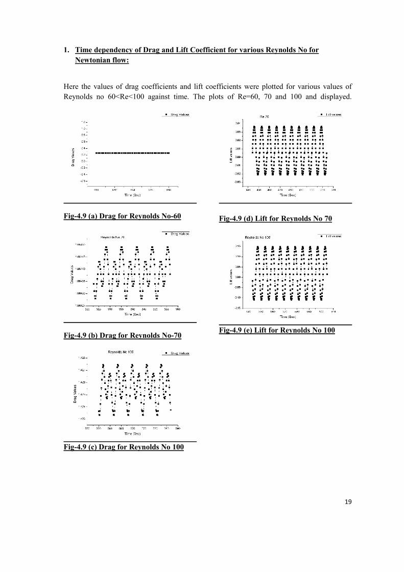
1. Time dependency of Drag and Lift Coefficient for various Reynolds No for

Newtonian flow:

Here the values of drag coefficients and lift coefficients were plotted for various values of

Reynolds no 60<Re<100 against time. The plots of Re=60, 70 and 100 and displayed.

Fig-4.9 (a) Drag for Reynolds No-60

Fig-4.9 (b) Drag for Reynolds No-70

Fig-4.9 (c) Drag for Reynolds No 100

Fig-4.9 (d) Lift for Reynolds No 70

Fig-4.9 (e) Lift for Reynolds No 100

20

It was found that the drag for Re-60 is remaining constant that is Steady State is still

remaining for Re-60. Thus, we need not need to calculate RMS value of lift or Strouhal No.

Nut further work needs to be done in order to determine at what point between Fig.76-83 lies

the onset of unsteadiness exists.

It was also observed from the plot of Drag and Lift with time that time necessary for

completion of one cycle of lift is more or less same to the time necessary for the drag to

complete two cycles. Thus, the frequency of Drag cycle is twice that of the lift. The

frequency with which lift varies is called the vortex shedding frequency. So, the drag

frequency is twice the vortex shedding frequency

2. Instantaneous Streamlines and Velocity Magnitude for various Reynolds No for

Newtonian flow:

The left plots denote the instantaneous streamlines for increasing Reynolds No. Though we

have the plots for all the intermediate values but the plots of the extreme values are shown.

And the right plots are for the instantaneous Velocity Magnitude of the Reynolds No-70 and

100. This is done to cover the entire regime

Fig-4.10 (a) Streamlines for Re-70

Fig-4.10 (b) Streamlines for Re-100

Fig-4.10 (c) Velocity Mag. For Re-70

Fig-4.10 (d)VelocityMag. For Re-100

This is of importance as the flow profile and the velocity profile would be viewed.

21

3. Post Processing of Results

This section is dedicated for the post-processing part. As it was already mentioned that

drag and lift coefficients are time dependent. So, for studying the impact of these

coefficients we need to determine tie average value of Drag and RMS value of lift.

Table-4.2 (Average Drag, RMS

Value of Lift and Strouhal No vs.

Reynolds No for Newtonian flow:

Reynolds No

Average Drag

RMS Value of Lift

Strouhal No

70 1.0644 0.0216 0.1428

80 1.1840 0.0445 0.1471

90 1.3043 0.0672 0.1515

100 1.4255 0.0933 0.1613

Fig-4.11 (a) Average Drag vs. Re

Fig-4.11 (b) RMS Lift vs. Reynolds No

Fig-4.11 (c) Strouhal No vs. Re

The values of Average drag and Root Mean Square value of Lift Coefficient were determined

after approximately 10 stable cycles were formed.

The average and RMS value of the coefficient were found for say 11th cycle. All the

mentioned values are increasing with the increase of Reynolds No.

22

4. Time Dependency of Drag and Lift Coefficient for various Reynolds No for non-

Newtonian flow(n=0.5):

Now, similar studies are shown for non-Newtonian fluids. Here also drag and lift coefficients

are plotted for various Reynolds number for different instances of time 60<Re <100.

Fig-4.12 (a) Drag for Re-60

Fig-4.12 (b) Drag for Re-100

Fig-4.12 (c) Lift for Re-60

Fig-4.12 (d) Lift for Re-100

Now for the non-Newtonian part similar simulation processes were done. But, we are quite

fortunate to obtain the time dependency of drag starting from Reynolds No 60. So for all the

values >60 the fluid remains in steady state conditions. For further post-processing time

dependency of lift was demonstrated.

It was also observed from the plot of Drag and Lift with time that time necessary for

completion of one cycle of lift is more or less same to the time necessary for the drag to

complete two cycles. Thus, the frequency of Drag cycle is twice that of the lift. The

frequency with which lift varies is called the vortex shedding frequency. So, the drag

frequency is twice the vortex shedding frequency

23

5. Instantaneous Streamlines and Velocity Magnitude for various Reynolds No for

non-Newtonian flow(n=0.5) :

Here on the left part we have stream functions and on the right we have velocity

magnitude for Re 60 and Re 100. The terminal points are taken to demonstrate the change

in flow pattern over entire domain.

4.13 (a) Stream Function Re-60

4.13 (a) Stream Function Re-100

4.13 (c) Velocity Magnitude Re 60

4.13 (d) Velocity Magnitude 60

The left plots denote the instantaneous streamlines for increasing Reynolds No. Though we

have the plots for all the intermediate values but the plots of the extreme values are shown.

And the right plots are for the instantaneous Velocity Magnitude of the Reynolds No-60 and

100. This is done to cover the entire regime.

24

6. Post Processing of Results

This section is dedicated for the post-processing part. As it was already mentioned that

drag and lift coefficients are time dependent. So, for studying the impact of these

coefficients we need to determine tie average value of Drag and RMS value of lift.

Table-4.3 Average Drag, RMS Value of Lift and Strouhal No vs. Reynolds No for Non-

Newtonian flow(n=0.5):

Reynolds No

Average Drag

RMS Value of Lift

Strouhal No

60 1.33977 0.013391 0.111111

70 1.44735 0.040897 0.1162790

80 1.55755 0.065023 0.1219512

90 1.66599 0.09104 0.13157894

100 1.76360 0.120721 0.14285714

Fig-4.14(a) Average Drag vs. Re

Fig-4.14 (b) RMS Lift vs. Re

Fig-4.14(c) Strouhal No vs. Re

Now, for the post-processing part the average value of Drag Coefficient, RMS value of Lift

Coefficient and the Strouhal number is plotted as a function of Reynolds No. It was observed

that as the Reynolds no increases all the values are increasing, this is in accordance with the

physics of the problem that as Reynolds no increases the flow shifts from Laminar to

Turbulent Regime and thus the values of Drag and Lift and in turn Strouhal would be

increasing for both Newtonian and non-Newtonian Fluid with an increase in the Reynolds no

25

Also, it was observed that at for constant value of Reynolds no we obtain different value of

Average Drag, RMS value of Lift and Strouhal no. This is due to the fact that with change of

power law index the nature and behaviour of fluid changes. Also, it was observed that

Average Drag and RMS value of lift is higher in case of non-Newtonian fluid but the value of

Strouhal no is higher for Newtonian fluid for same value of the Reynolds no.

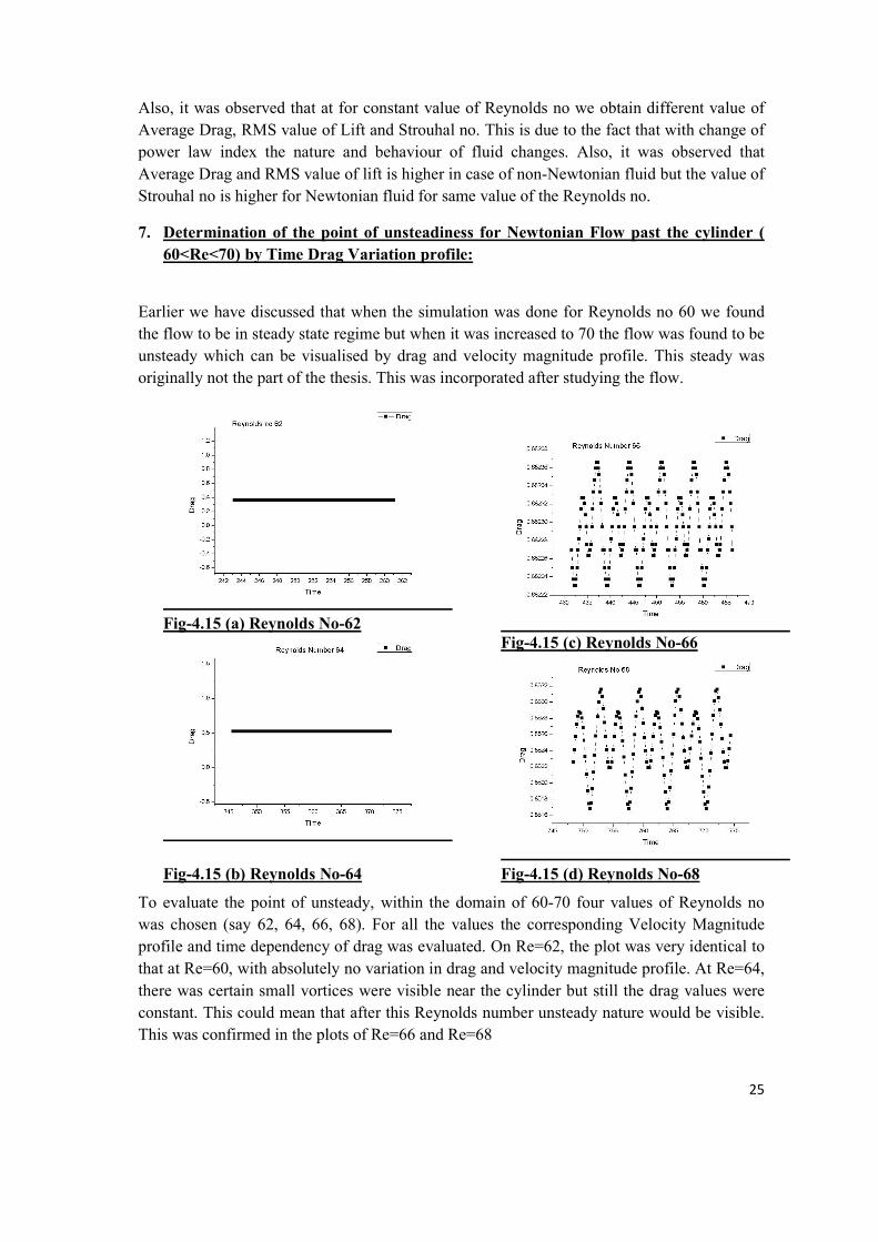
7. Determination of the point of unsteadiness for Newtonian Flow past the cylinder (

60<Re<70) by Time Drag Variation profile:

Earlier we have discussed that when the simulation was done for Reynolds no 60 we found

the flow to be in steady state regime but when it was increased to 70 the flow was found to be

unsteady which can be visualised by drag and velocity magnitude profile. This steady was

originally not the part of the thesis. This was incorporated after studying the flow.

Fig-4.15 (a) Reynolds No-62

Fig-4.15 (b) Reynolds No-64

Fig-4.15 (c) Reynolds No-66

Fig-4.15 (d) Reynolds No-68

To evaluate the point of unsteady, within the domain of 60-70 four values of Reynolds no

was chosen (say 62, 64, 66, 68). For all the values the corresponding Velocity Magnitude

profile and time dependency of drag was evaluated. On Re=62, the plot was very identical to

that at Re=60, with absolutely no variation in drag and velocity magnitude profile. At Re=64,

there was certain small vortices were visible near the cylinder but still the drag values were

constant. This could mean that after this Reynolds number unsteady nature would be visible.

This was confirmed in the plots of Re=66 and Re=68

26

8. Determination of the point of unsteadiness for Newtonian Flow past the cylinder (

60<Re<70) by Velocity Magnitude profile:

Though the drag plots were quite clearly visible to have taken its natural form of cyclic

variation with time but, the velocity profile still velocity profile doesn’t have full unsteady

character for Re=66. But, we can see fully unsteady for Re=68.

Fig.4.16 (a) Reynolds No-62

Fig.4.16 (b) Reynolds No-64

Fig.4.16 (c) Reynolds No-66

Fig.4.16 (d) Reynolds No-68

So, it can be argued that within the range of 64-66 the point of unsteady exists and this can be

point of further research to determine exactly where that is.

27

5) Conclusions

There are numerous conclusions that can be drawn from sets of experimentation and

simulations that can be visualised.

For the square cavity problem, the result obtained for both Newtonian and non-Newtonian

was in well accordance with the ones in literature. This means the simulation setup was close

approximation of the real time problem.

For the steady state flow across a cylinder, the value of drag was consistent with the ones in

literature for both Newtonian and non-Newtonian flows.

Now, for unsteady flow around a circular cylinder, the time dependency of drag and lift

coefficients were visible for Re>70 for Newtonian and Re>60 for non-Newtonian fluids.

Hence, the non-Newtonian fluids have a tendency to attain unsteady state at smaller Reynolds

Number. Further, the drag frequency is twice the lift/vortex shedding frequency. The Average

value of Drag, RMS value of Lift and Strouhal no were increasing with increase in Reynolds

no for both Newtonian and Non-Newtonian fluids. But, at constant Reynolds no the value of

average drag and RMS lift is higher for Non-Newtonian flow but Strouhal no had higher

value of Newtonian flow.

The point of unsteady was evaluated from velocity magnitude profile and drag vs. time plot.

And it was found to be in a range of 64-66 for Newtonian flow.

28

6) Bibliography

[1] D. J. Tritton.: Experiments on the flow past a circular cylinder at low Reynolds number. J. Fluid Mech.6,

547–567 (1959).

[2] S. C. R. Dennis and G. Z. Chang: Numerical solutions for steady flow past a circular cylinder at Reynolds

numbers up to 100. J. Fluid Mech.42, 471–489 (1970).

[3] B. Fornberg.: A numerical study of steady viscous flow past a circular cylinder. J. Computational Physics

98, 819–855 (1980).

[4] B. Fornberg.: Steady viscous flow past a circular cylinder up to Reynolds number 600. J. Computational

Physics 61, 297–320 (1985).

[5] D. H. Peregrine.: A note on the steady high-Reynolds-number flow about a circular cylinder. J. Fluid

Mech.157, 493–500 (1985).

[6] P. W. Bearman, Vortex shedding from oscillating bluff bodies, Ann. Rev. Fluid Mech., 16 (1984) 195-222.

[7] B. Cantwell and D. Coles, An experimental study of entrainment and transport in the turbulent near wake of

a circular cylinder, J. Fluid Mech., 136 (1983) 321-374.

[8] J S Son and T J Hanratty, Numerical solution for the flow around a cylinder at Reynolds number of 40,

200,500, J. Fluid Mech., 35 (2) (1969) 369-386.

[9] M. Braza, P. Chassaing and H.H. Minh, Numerical study and physical analysis of the pressure and velocity

fields in the near wake of a circular cylinder, J. Fluid Mech., 165 (1986) 79- 130.

[10] Y. Lecointe and J. Piquet, Flow structure in the wake of an oscillating cylinder, J. Fluid Eng., 111 (1989)

139-148.

[11] R.P. Chhabra, J.F. Richardson, Non-Newtonian Flow and Applied Rheology: Engineering Applications,

second ed., Butterworth-Heinemann, Oxford, 2008.

[12] R.P. Chhabra, Bubbles, Drops and Particles in Non-Newtonian Fluids, seconded., CRC Press, Boca Raton,

FL, 2006.

[13] W.R. Schowalter, Mechanics of Non-Newtonian Fluids, Pergamon, Oxford, UK,1977.

[14] M.M. Zdravkovich, Flow Around Circular Cylinders Fundamentals, vol. 1, Oxford University Press, New

York, 1997.

[15] M.M. Zdravkovich, Flow Around Circular Cylinders Applications, vol. 2, Oxford University Press, New

York, 2003.

[16] R. Clift, J. Grace, M.E. Weber, Bubbles, Drops and Particles, Academic, New York, 1978.

[17] R. I. Tanner: Stokes paradox for power-law flow around a cylinder. J. Non–Newtonian Fluid Mech.50,

217–224 (1993).

[18] E. Morsic.: On the Stokes paradox for power law fluids. Z. Angew. Math. Mech. (ZAMM) 81, 31–36

(2001).

[19] M. J. Whitney, G. J. Rodin : Force-velocity relationships for rigid bodies translating through unbounded

shear-thinning power-law fluids. Int. J. Non-Linear Mech.36, 947–953 (2001).

29

[20] S.J.D. D’Alessio., J.P. Pascal: Steady flow of a power-law fluid past a cylinder. Acta Mech.117, 87–100

(1996).

[21] H. Takami,, H.B. Keller.: Steady two-dimensional viscous flow of an incompressible fluid past a circular

cylinder. High-Speed Computing in Fluid Dynamics - The Physics of Fluids, Suppl. II, 51–56 (1969).

[22] P. Anagnostopoulos, G. Iliadis.: Numerical study of the blockage effects on viscous flow past a circular

cylinder. Int. J. Num. Meth. Fluids22, 1061–1074 (1996).

[23] P. K. Stansby, A. Slaouti.: Simulation of vortex shedding including blockage by the rando-vortex and other

methods. Int. J. Num. Meth. Fluids17, 1003–1013 (1993).

[24] P. Y. Huang, J. Feng.: Wall effects on the flow of viscoelastic fluids around a circular cylinder. J. Non–

Newtonian Fluid Mech.60, 179–198 (1995).

[25] R.P. Chhabra, K. Rami., P. H T, Uhlherr.: Drag on cylinders in shear thinning viscoelastic liquids. Chem.

Eng. Sci. 56, 2221–2227 (2001).

[26] K. N. Ghia, W. L. Hankey AND J. K. Hodge, “Study of Incompressible Navier-Stokes Equations in

Primitive Variables Using Implicit Numerical Technique,” AIAA Paper No. 77-648, 1977; AIAA J. 17(3)

(1979), 298.

[27] S. G. Rubin , P. K. Khosla, J. Comput. Phys. 24(3) (1977) 217.

[28] R. E. Smith, A. Kidd, “Comparative Study of Two Numerical Techniques for the Solution of

Viscous Flow in a Driven Cavity,” pp. 61-82, NASA SP-378, 1975.

[29] K. N. Ghia, C. T. Shin, AND U. Ghia, “Use of Spline Approximations for Higher-Order Accurate

Solutions of Navier-Stokes Equations in Primitive Variables,” AIAA Paper No. 79-1467, 1979.

[30] M. Nallaswamy AND K. K. Prasad, J. Fluid Mech. 79(2) (1977), 391.

[31] R. K. Agarwal, “A Third-Order-Accurate Upwind Scheme for Navier-Stokes Solutions at High

Reynolds Numbers,” AIAA Paper No. 8 l-01 12, 1981.

[32] U. Ghia, K. N. Ghia AND C. T. Shin, “High-Re Solutions for Incompressible Flow Using the

Navier-Stokes Equations and a Multigrid Method” J. comput phs 48, 387-411 (1982)

[33] P. Neofytou, “A 3rd order upwind finite volume method for generalised Newtonian fluid flows” Advances

in Engineering Software 36 (2005) 664–680

[34] P. Sivakumar, R. P. Bharti, R.P. Chhabra, “Effect of power-law index on critical parameters for power-law

flow across an unconfined circular cylinder” Chemical Engineering Science 61 (2006) 6035 – 6046

[35] P. Koteswara Rao, C. Sasmal, A.K. Sahu, R.P. Chhabra, V. Eswaran, “Effect of power-law fluid behaviour

on momentum and heat transfer characteristics of an inclined square cylinder in steady flow regime”

International J. Heat Mass Transfer 54 (2011) 2854–2867.

[36] M. Coutanceau, J. R. Defaye, Circular Cylinder Wake Configurations – A Flow Visualization Survey,

Appl. Mech. Rev., 44(6), June 1991.

Two Dimensional flow of Shear Thinning Fluid around a ...

Documents

Transcript of Two Dimensional flow of Shear Thinning Fluid around a ...