Two advances in GP-based prediction and …...Introduction The q-points Expected Improvement Bonus:...
49
Introduction The q-points Expected Improvement Bonus: symmetrical covariance kernels Two advances in GP-based prediction and optimization for computer experiments David Ginsbourger Institut de Math ´ ematiques & Centre d’Hydrog ´ eologie, Universit ´ e de Neuch ˆ atel, and Ecole Nat. Sup. des Mines de Saint-Etienne (Ph.D. defense coming soon :) Journ´ ees du GdR MASCOT-NUM, Day 1 (18/03/2009) University Paris XIII - Galil´ ee institute [email protected] GDR Mascot Num, 18/03/09
Transcript of Two advances in GP-based prediction and …...Introduction The q-points Expected Improvement Bonus:...

Introduction
The q-points Expected Improvement
Bonus: symmetrical covariance kernels
Two advances in GP-based prediction and
optimization for computer experiments
David Ginsbourger
Institut de Mathematiques & Centre d’Hydrogeologie, Universite de Neuchatel,and Ecole Nat. Sup. des Mines de Saint-Etienne (Ph.D. defense coming soon :)
Journees du GdR MASCOT-NUM, Day 1 (18/03/2009)
University Paris XIII - Galilee institute
[email protected] GDR Mascot Num, 18/03/09

Introduction
The q-points Expected Improvement
Bonus: symmetrical covariance kernels
Motivations
Outline
1 Introduction
Motivations
2 The q-points Expected Improvement
Definition and basic properties
Derivation of the q-EI (cases q = 2 and q > 2)
Approximate optimization of the q-EI
3 Bonus: covariance kernels for predicting symmetrical functions
Kernels for GP with Invariant Realizations
Applications: simulating and interpolating invariant functions
[email protected] GDR Mascot Num, 18/03/09

Introduction
The q-points Expected Improvement
Bonus: symmetrical covariance kernels
Motivations
General context
Amazing growth of computing power in numerical simulation
Powerful processors, clustering.
Scientific computing has reached maturity: FEM, Monte-Carlo, etc.
Paradox: since one always want more accurate results, computation
times are often stagnating and even sometimes increasing!
Examples of application domains
Crash-test simulation: ≈ 20h per ”run”
Nuclear plant: > 1hr to estimate neutronic criticality of a set of fuel rods
Simulation of the behaviour of a CO2 bubble stocked during 10000
years in a natural geological reservoir: several days.
[email protected] GDR Mascot Num, 18/03/09
Introduction
The q-points Expected Improvement
Bonus: symmetrical covariance kernels
Motivations
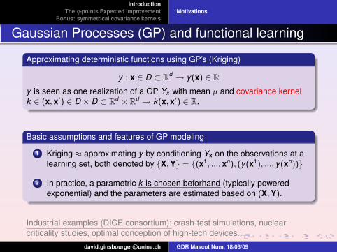
Gaussian Processes (GP) and functional learning
Approximating deterministic functions using GP’s (Kriging)
y : x ∈ D ⊂ Rd → y(x) ∈ R
y is seen as one realization of a GP Yx with mean µ and covariance kernel
k ∈ (x, x′) ∈ D × D ⊂ Rd × R
d → k(x, x′) ∈ R.
Basic assumptions and features of GP modeling
1 Kriging ≈ approximating y by conditioning Yx on the observations at a
learning set, both denoted by X,Y = (x1, ..., xn), (y(x1), ..., y(xn))
2 In practice, a parametric k is chosen beforhand (typically powered
exponential) and the parameters are estimated based on (X,Y).
Industrial examples (DICE consortium): crash-test simulations, nuclear
criticality studies, optimal conception of high-tech devices...
[email protected] GDR Mascot Num, 18/03/09

Introduction
The q-points Expected Improvement
Bonus: symmetrical covariance kernels
Motivations
Example of Ordinary Kriging Interpolation
Interpolation (right) of Branin’s function (left), known at 9 points (in red).
The kernel is k(x, x′) = σ2e−∑ 2
j=1
(xj−x′
jψj
)2
with (σ2, ψ) estimated by ML
[email protected] GDR Mascot Num, 18/03/09

Introduction
The q-points Expected Improvement
Bonus: symmetrical covariance kernels
Motivations
Ordinary Kriging Equations
A central property of OK, when k is known (and µ has a U(R) prior...)
[Y (x)|Y (X) = Y] ∼ N(
m(x), s2(x))
m(x) = E[Y (x)|Y (X) = Y] = µ + k(x)T K−1 (Y − µn)
s2(x) = Var [Y (x)|Y (X) = Y] = σ2 − k(x)T K−1k(x) +
(1−
Tn K−1k(x)
)2
(
Tn K−1n
)
µ =
T K−1Y
(T K−1), K =
k(x1, x1) k(x1, x2) ... k(x1, xn)k(x2, x1) k(x2, x2) ... k(x2, xn)
... ... .... ....
k(xn, x1) ... .... k(xn, xn)
and k(x) =
k(x, x1)k(x, x2)
...
k(x, xn)
[email protected] GDR Mascot Num, 18/03/09

Introduction
The q-points Expected Improvement
Bonus: symmetrical covariance kernels
Motivations
The Expected improvement (EI) criterion
Expected Improvement
EI(x) = E[(min(Y (X)) − Y (x))+ |Y (X) = Y
]
M. Schonlau, W.J. Welch and D.R. Jones.
Efficient Global Optimization of ExpensiveBlack-box Functions
Journal of Global Optimization, 1998.
EI(x) = (min(y(X))−m(x)) Φ
(min(y(X))−m(x)
s(x)
)+ s(x)φ
(min(y(X))−m(x)
s(x)
),
where Φ and φ are the cdf and pdf of the standard gaussian law, respectively.
[email protected] GDR Mascot Num, 18/03/09

Introduction
The q-points Expected Improvement
Bonus: symmetrical covariance kernels
Motivations
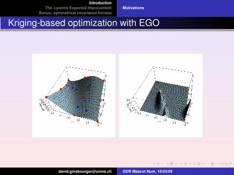
Kriging-based optimization with EGO
[email protected] GDR Mascot Num, 18/03/09

Introduction
The q-points Expected Improvement
Bonus: symmetrical covariance kernels
Motivations
Kriging-based optimization with EGO
[email protected] GDR Mascot Num, 18/03/09

Introduction
The q-points Expected Improvement
Bonus: symmetrical covariance kernels
Motivations
Kriging-based optimization with EGO
[email protected] GDR Mascot Num, 18/03/09
Introduction
The q-points Expected Improvement
Bonus: symmetrical covariance kernels
Motivations
Kriging-based optimization with EGO
[email protected] GDR Mascot Num, 18/03/09

Introduction
The q-points Expected Improvement
Bonus: symmetrical covariance kernels
Motivations
Kriging-based optimization with EGO
[email protected] GDR Mascot Num, 18/03/09

Introduction
The q-points Expected Improvement
Bonus: symmetrical covariance kernels
Motivations
Kriging-based optimization with EGO
[email protected] GDR Mascot Num, 18/03/09

Introduction
The q-points Expected Improvement
Bonus: symmetrical covariance kernels
Motivations
Kriging-based optimization with EGO: results
[email protected] GDR Mascot Num, 18/03/09

Introduction
The q-points Expected Improvement
Bonus: symmetrical covariance kernels
Motivations
EGO: a sequential procedure
Sketch of the EGO Algorithm
1: function EGO(X, Y, p)2: for i ← 1, p do3: xnew
i= argmaxx∈DEI(x) ⊲ with updated X and Y
4: X = X⋃xnew
i
5: Y = Y⋃y(xnew
i) ⊲ with updated X and Y
6: Update the covariance parameters and the kriging model7: end for8: end function
Major issue with sequentiality:
In industrial context, the project duration is more crucial than computation
time, provided that the latter can be distributed on multiple processors.
Algorithms such as EGO may be wasteful... they need to be parallelized!
Question: how to evaluate the added value of sampling q points?
[email protected] GDR Mascot Num, 18/03/09

Introduction
The q-points Expected Improvement
Bonus: symmetrical covariance kernels
Definition and basic properties
Derivation of the q-EI (cases q = 2 and q > 2)
Approximate optimization of the q-EI
Outline
1 Introduction
Motivations
2 The q-points Expected Improvement
Definition and basic properties
Derivation of the q-EI (cases q = 2 and q > 2)
Approximate optimization of the q-EI
3 Bonus: covariance kernels for predicting symmetrical functions
Kernels for GP with Invariant Realizations
Applications: simulating and interpolating invariant functions
[email protected] GDR Mascot Num, 18/03/09

Introduction
The q-points Expected Improvement
Bonus: symmetrical covariance kernels
Definition and basic properties
Derivation of the q-EI (cases q = 2 and q > 2)
Approximate optimization of the q-EI
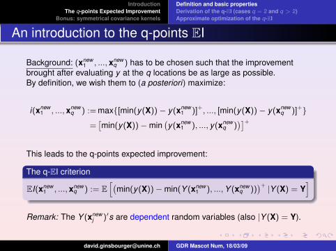
An introduction to the q-points EI
Background: (xnew1 , ..., xnew
q ) has to be chosen such that the improvement
brought after evaluating y at the q locations be as large as possible.
By definition, we wish them to (a posteriori) maximize:
i(xnew1 , ..., xnew
q ) := max[min(y(X)) − y(xnew1 )]+, ..., [min(y(X)) − y(xnew
q )]+
=[min(y(X)) − min
(y(xnew
1 ), ..., y(xnewq )
)]+
This leads to the q-points expected improvement:
The q-EI criterion
EI(xnew1 , ..., xnew
q ) := E
[(min(y(X)) − min(Y (xnew
1 ), ...,Y (xnewq ))
)+|Y (X) = Y
]
Remark: The Y (xnewj )′s are dependent random variables (also |Y (X) = Y).
[email protected] GDR Mascot Num, 18/03/09
Introduction
The q-points Expected Improvement
Bonus: symmetrical covariance kernels
Definition and basic properties
Derivation of the q-EI (cases q = 2 and q > 2)
Approximate optimization of the q-EI
An introduction to the q-points EI
Background: (xnew1 , ..., xnew
q ) has to be chosen such that the improvement
brought after evaluating y at the q locations be as large as possible.
By definition, we wish them to (a posteriori) maximize:
i(xnew1 , ..., xnew
q ) := max[min(y(X)) − y(xnew1 )]+, ..., [min(y(X)) − y(xnew
q )]+
=[min(y(X)) − min
(y(xnew
1 ), ..., y(xnewq )
)]+
This leads to the q-points expected improvement:
The q-EI criterion
EI(xnew1 , ..., xnew
q ) := E
[(min(y(X)) − min(Y (xnew
1 ), ...,Y (xnewq ))
)+|Y (X) = Y
]
Remark: The Y (xnewj )′s are dependent random variables (also |Y (X) = Y).
[email protected] GDR Mascot Num, 18/03/09

Introduction
The q-points Expected Improvement
Bonus: symmetrical covariance kernels
Definition and basic properties
Derivation of the q-EI (cases q = 2 and q > 2)
Approximate optimization of the q-EI
An illustration of the 2-points EI
Figure: 1 and 2-EI associated with a 2d degree polynom
The 2-EI optimal couple is here made of 2 local maxima of the 1-EI
[email protected] GDR Mascot Num, 18/03/09

Introduction
The q-points Expected Improvement
Bonus: symmetrical covariance kernels
Definition and basic properties
Derivation of the q-EI (cases q = 2 and q > 2)
Approximate optimization of the q-EI
An illustration of the 2-points EI
Figure: 1 and 2-EI associated with a 1-dimensional linear function.
Now, the 2-EI optimal couple is made of two points around the 1-EI maximizer.
[email protected] GDR Mascot Num, 18/03/09

Introduction
The q-points Expected Improvement
Bonus: symmetrical covariance kernels
Definition and basic properties
Derivation of the q-EI (cases q = 2 and q > 2)
Approximate optimization of the q-EI
q-EI optimal designs?
Xnew∗ = argmaxxnew1
,...,xnewq ∈S EI
(xnew
1 , ..., xnewq
)
This optimization is in dimension dq. Typically, dq ≥ 100
Since the objective function is noisy (empirical EI, computed by Monte-Carlo
method) and derivative-free, the problem is not straightforward.
First proposed approach
Solve the problem in a greedy way, in feeding the Kriging model with arbitrary
values (Kriging Believer and Constant Liar heuristic strategies).
[email protected] GDR Mascot Num, 18/03/09

Introduction
The q-points Expected Improvement
Bonus: symmetrical covariance kernels
Definition and basic properties
Derivation of the q-EI (cases q = 2 and q > 2)
Approximate optimization of the q-EI
One heuristic strategy for the cases where q > 2
Constant Liar
The model is sequentially updated in setting the unkwown y(xnewi ) values
equal to a fixed constant L ∈ R:
1: function CL(X, Y, L, q)2: for i ← 1, q do3: xnew
i= argmaxx∈DEI(x) ⊲ with updated X and Y
4: X = X⋃xnew
i
5: Y = Y⋃L
6: end for7: end function
The constant L allows the user to control the repulsion created by the sequentially
visited points (L = max(Y) for a strong repulsion, L = min(Y) for a smooth repulsion)
[email protected] GDR Mascot Num, 18/03/09
Introduction
The q-points Expected Improvement
Bonus: symmetrical covariance kernels
Definition and basic properties
Derivation of the q-EI (cases q = 2 and q > 2)
Approximate optimization of the q-EI
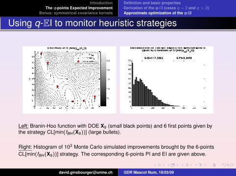
Using q-EI to monitor heuristic strategies
Left: Branin-Hoo function with DOE X9 (small black points) and 6 first points given bythe strategy CL[min(fBH(X9))] (large bullets).
Right: Histogram of 103 Monte Carlo simulated improvements brought by the 6-points
CL[min(fBH(X9))] strategy. The corresponding 6-points PI and EI are given above.
[email protected] GDR Mascot Num, 18/03/09

Introduction
The q-points Expected Improvement
Bonus: symmetrical covariance kernels
Definition and basic properties
Derivation of the q-EI (cases q = 2 and q > 2)
Approximate optimization of the q-EI
A 6-dimensional case study: the ”Hartmann” function
y(x) = −4∑
j=1
cj × exp
(−
6∑
i=1
ai,j × (xi − pi,j)2
)
a =
10.00 0.05 3.00 17.003.00 10.00 3.50 8.00
17.00 17.00 1.70 0.053.50 0.10 10.00 10.001.70 8.00 17.00 0.108.00 14.00 8.00 14.00
p =
0.1312 0.2329 0.2348 0.40470.1696 0.4135 0.1451 0.88280.5569 0.8307 0.3522 0.87320.0124 0.3736 0.2883 0.57430.8283 0.1004 0.3047 0.10910.5886 0.9991 0.6650 0.0381
c =
1.01.23.03.2
global minimum =−3.32
global minimizer = [0.202, 0.150, 0.477, 0.275, 0.312, 0.657]
[email protected] GDR Mascot Num, 18/03/09
Introduction
The q-points Expected Improvement
Bonus: symmetrical covariance kernels
Definition and basic properties
Derivation of the q-EI (cases q = 2 and q > 2)
Approximate optimization of the q-EI
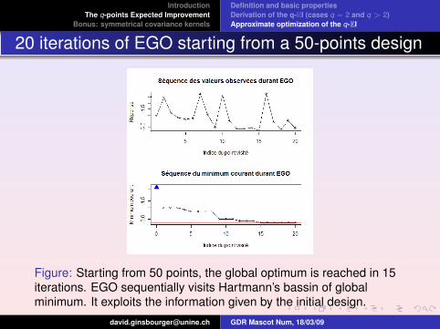
20 iterations of EGO starting from a 50-points design
Figure: Starting from 50 points, the global optimum is reached in 15
iterations. EGO sequentially visits Hartmann’s bassin of global
minimum. It exploits the information given by the initial design.
[email protected] GDR Mascot Num, 18/03/09

Introduction
The q-points Expected Improvement
Bonus: symmetrical covariance kernels
Definition and basic properties
Derivation of the q-EI (cases q = 2 and q > 2)
Approximate optimization of the q-EI
90 iterations of EGO starting from a 10-points design
Figure: EGO find the minimum in 36 iterations: fast if we consider
that X has only 10 points. The sequence is here more exploratory.
[email protected] GDR Mascot Num, 18/03/09
Introduction
The q-points Expected Improvement
Bonus: symmetrical covariance kernels
Definition and basic properties
Derivation of the q-EI (cases q = 2 and q > 2)
Approximate optimization of the q-EI
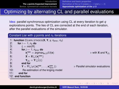
Optimizing by alternating CL and parallel evaluations
Idea: parallel synchronous optimization using CL at every iteration to get q
explorations points. The lies of CL are corrected at the end of each iteration,
after the parallel evaluations of the simulator.
Constant Liar with q points and nit iterations
1: function CLMIN.STAGES(X, Y, y, nproc , nit )2: for i ← 1, nit do3: L = min(Y)4: for j ← 1, nproc do5: xnew
j= argmaxx∈DEI(x) ⊲ with X and YCL
6: X = X⋃xnew
j
7: YCL = Y⋃L
8: end for9: Y = Y
⋃y(xnew
1, . . . , xnew
nproc) ⊲ Parallel simulator evaluations
10: Re-estimation of the kriging model11: end for12: end function
[email protected] GDR Mascot Num, 18/03/09

Introduction
The q-points Expected Improvement
Bonus: symmetrical covariance kernels
Definition and basic properties
Derivation of the q-EI (cases q = 2 and q > 2)
Approximate optimization of the q-EI
CL with 10 proc. in parallel, 50 initial points
Figure: The minimum is reached in 5 time units!
[email protected] GDR Mascot Num, 18/03/09

Introduction
The q-points Expected Improvement
Bonus: symmetrical covariance kernels
Definition and basic properties
Derivation of the q-EI (cases q = 2 and q > 2)
Approximate optimization of the q-EI
CL with 10 proc. in parallel, 50 initial points
Figure: The algorithm alternates between a first exploration phase
(two first time units), a more exploratory phase (3rd et 4th time units),
and a final exploitation phase during which it finds the minimum.
[email protected] GDR Mascot Num, 18/03/09

Introduction
The q-points Expected Improvement
Bonus: symmetrical covariance kernels
Definition and basic properties
Derivation of the q-EI (cases q = 2 and q > 2)
Approximate optimization of the q-EI
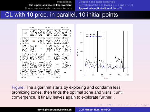
CL with 10 proc. in parallel, 10 initial points
Figure: Starting from a 10-points design, CLmin with 10 processors
finds the minimum in 7 time units.
[email protected] GDR Mascot Num, 18/03/09
Introduction
The q-points Expected Improvement
Bonus: symmetrical covariance kernels
Definition and basic properties
Derivation of the q-EI (cases q = 2 and q > 2)
Approximate optimization of the q-EI
CL with 10 proc. in parallel, 10 initial points
Figure: The algorithm starts by exploring and condamn less
promizing zones, then finds the optimal zone and visits it until
convergence. It finally leaves again to explorate further...
[email protected] GDR Mascot Num, 18/03/09

Introduction
The q-points Expected Improvement
Bonus: symmetrical covariance kernels
Definition and basic properties
Derivation of the q-EI (cases q = 2 and q > 2)
Approximate optimization of the q-EI
Conclusion and perspectives for the q − EI
Experimental feed-back
Computing kriging-based multipoints criteria by MC is affordable
whatever the dimension of the space of inputs
The Constant Liar heuristic strategy gave very promizing results on 1-,
2-, and 6-dimensional toy examples
Tracks for future works
Apply these tools to real world problems (currently done with a nuclear
safety application)
Optimize the q-EI (mutating good candidate designs ?)
[email protected] GDR Mascot Num, 18/03/09

Introduction
The q-points Expected Improvement
Bonus: symmetrical covariance kernels
Kernels for GP with Invariant Realizations
Applications: simulating and interpolating invariant functions
Outline
1 Introduction
Motivations
2 The q-points Expected Improvement
Definition and basic properties
Derivation of the q-EI (cases q = 2 and q > 2)
Approximate optimization of the q-EI
3 Bonus: covariance kernels for predicting symmetrical functions
Kernels for GP with Invariant Realizations
Applications: simulating and interpolating invariant functions
[email protected] GDR Mascot Num, 18/03/09

Introduction
The q-points Expected Improvement
Bonus: symmetrical covariance kernels
Kernels for GP with Invariant Realizations
Applications: simulating and interpolating invariant functions
Aim of this work
Industrial problem:
Let us assume that a set of physical symmetries leave y unchanged
...how can we take it into account within GP techniques?
Mathematical formulation:
if G is a finite groupe acting on D via
Φ : (x, g) ∈ D × G −→ Φ(x, g) = g.x ∈ D
what properties must k satisfy for Yx to have its paths invariant by Φ?
[email protected] GDR Mascot Num, 18/03/09

Introduction
The q-points Expected Improvement
Bonus: symmetrical covariance kernels
Kernels for GP with Invariant Realizations
Applications: simulating and interpolating invariant functions
Main property
Definition Y has its paths invariant under the action Φ if
∀ω ∈ Ω, ∀x ∈ D, ∀g ∈ G, Yx(ω) = Yg.x(ω)
Theorem: Let Y be a centered process (not necessarily gaussian!!!)
Y has invariant paths under Φ (up to a modification)
⇔∃ a d.p. kernel kZ such that kY (x, x′) =
∑(g,g′)∈G2 kZ (g.x, g′.x′)
[email protected] GDR Mascot Num, 18/03/09

Introduction
The q-points Expected Improvement
Bonus: symmetrical covariance kernels
Kernels for GP with Invariant Realizations
Applications: simulating and interpolating invariant functions
Application: A smooth symmetrical 2-D GP
Idea: to build processes with paths invariant under Φ on the basis of a
stationary process Y , by simply symmetrizing it:
∀x ∈ D, YΦx =
1
2(Yx + Ys(x)) =
1
2(Y(x1,x2) + Y(x2,x1))
The covariance kernel of the new process Y Φ is given by:
kXΦ (x, x
′) =
1
4[kX (x − x
′) + kX (s(x) − x
′) + kX (x − s(x
′)) + kX (s(x) − s(x
′))]
=1
4
[e−||(x1−x′
1,x2−x′
2)||2
+ e−||(x1−x′
1,x′
2−x2)||2
+ e−||(x′
1−x1,x2−x′
2)||2
+ e−||(x′
1−x1,x
′2−x2)||2
]
Note that Y Φ inheritates from Y ’s smoothness, including on the axis of
symmetry x ∈ R2 : s(x) = x.
[email protected] GDR Mascot Num, 18/03/09

Introduction
The q-points Expected Improvement
Bonus: symmetrical covariance kernels
Kernels for GP with Invariant Realizations
Applications: simulating and interpolating invariant functions
Simulation of a smooth symmetrical 2-D GP
Figure: One path of GP with symmetrized Gaussian kernel
[email protected] GDR Mascot Num, 18/03/09

Introduction
The q-points Expected Improvement
Bonus: symmetrical covariance kernels
Kernels for GP with Invariant Realizations
Applications: simulating and interpolating invariant functions
Kriging with a symmetrized kernel
Figure: From left to right:
symmetrized Branin function (f ),
a 9-points DOE X obtained by i.i.d. uniform drawings on the square,
the DOE symmetrized from X with respect to f ’s axis of symmetry.
[email protected] GDR Mascot Num, 18/03/09

Introduction
The q-points Expected Improvement
Bonus: symmetrical covariance kernels
Kernels for GP with Invariant Realizations
Applications: simulating and interpolating invariant functions
Kriging with a symmetrized kernel
Figure: Kriging f on the basis of X (9 points), with Gaussian
covariance
ISE on a 21 × 21-elements test grid: 820.93
[email protected] GDR Mascot Num, 18/03/09

Introduction
The q-points Expected Improvement
Bonus: symmetrical covariance kernels
Kernels for GP with Invariant Realizations
Applications: simulating and interpolating invariant functions
Kriging with a symmetrized kernel
Figure: Kriging f on the basis of Xsym (18 points), with Gaussian
covariance
ISE on a 21 × 21-elements test grid: 694.11
[email protected] GDR Mascot Num, 18/03/09

Introduction
The q-points Expected Improvement
Bonus: symmetrical covariance kernels
Kernels for GP with Invariant Realizations
Applications: simulating and interpolating invariant functions
Kriging with a symmetrized kernel
Figure: Kriging on the basis of X, with symmetrized Gaussian
covariance
ISE on a 21 × 21-elements test grid: 330.26
[email protected] GDR Mascot Num, 18/03/09

Introduction
The q-points Expected Improvement
Bonus: symmetrical covariance kernels
Kernels for GP with Invariant Realizations
Applications: simulating and interpolating invariant functions
Conclusion and perspectives
It is not reasonable to make predictions using classical covariance kernels
when invariances under some group actions are known a priori.
Symmetrizing stationary kernels provides a convenient way of getting
invariant GPs with nice smoothness properties.
Future issues to be addressed include
investigating broader classes of invariant kernels
applying symmetrical Kriging to higher-dimensional industrial cases
learning symmetries from data
[email protected] GDR Mascot Num, 18/03/09
Introduction
The q-points Expected Improvement
Bonus: symmetrical covariance kernels
Kernels for GP with Invariant Realizations
Applications: simulating and interpolating invariant functions
Thank you for your Attention : )
Aknowledgments
L. Carraro (Telecom Saint-Etienne), A. Antoniadis (UJF), R. Le Riche
(CNRS), O. Roustant (Mines), R. Haftka (Florida), Y. Richet (IRSN), A.
Journel (Stanford), V. Picheny (Mines / Florida), P. Renard (UNINE).
This work was conducted within the frame of the DICE (Deep Inside Computer Experiments) Consortiumbetween ARMINES, Renault, EDF, IRSN, ONERA, and Total S.A.
[email protected] GDR Mascot Num, 18/03/09

Introduction
The q-points Expected Improvement
Bonus: symmetrical covariance kernels
Kernels for GP with Invariant Realizations
Applications: simulating and interpolating invariant functions
Any questions?
[email protected] GDR Mascot Num, 18/03/09