Twin Crises

A Reexamination of Empirical Links

Jürgen von Hagen∗ and Tai-kuang Ho∗∗

ZEI b, Center for European Integration Studies, University of Bonn

April 2003

1 Introduction Twin crises refer to the association of banking crises and balance-of-payments crises, and the vice

versa. We have witnessed several balance-of-payments crises that occurred in the midst of a banking crisis, like for instance, Chile in 1982, Finland in 1992, Sweden in 1992, Mexico in 1994, and the recent Asian financial crisis. It is commonly perceived that twin crises will become more frequent under the environment of increasing financial integration and volatile international capital mobility (Wyplosz, 1999).

Twin crises have attracted attention because they tend be more severe than individual banking and currency crises. Twin crises are associated with a larger economic recession and are more costly in terms of bailout cost. However, empirical research on twin crises is rather rare. Kaminsky and Reinhart (1996, 1999) were the first to investigate systematically the links between banking and currency crises. Subsequent work by Glick and Hutchison (2001) employed a much larger data set, which included 90 industrial and developing countries.

All these papers, however, suffer from a common methodological shortcoming. There is an asymmetry in the definition and identification of crises between the two fields of banking and currency markets. More specifically, they use market events like forced merger, bank closures or government intervention to identify banking crises. In contrast, they follow the recent literature on currency crises and develop an index of market pressure to identify currency crises. The currency-crises literature has shown that depending on market events to identify crises is problematic, as it identifies crises only, when they are severe enough to trigger market events such as large devaluations or the collapse of a fixed exchange rate regime. In contrast, crises that were successfully fended off are neglected. The index method is well accepted and considered superior. But if the reliance on market events biases the analysis of currency crises, it is likely to do so in the case of banking crises. We have showed in von Hagen and Ho (2003) that using an events method to identify banking crises is problematic, and the index method is applicable to the identification of banking crises. It is an interesting and important question whether such an unequal treatment of banking and currency crises had influenced the empirical results regarding twin crises. This is what we try to answer in this chapter. We treat banking and currency crises equally in terms of

∗ Center for European Integration Studies (ZEI B), Walter-Flex-Str. 3, D-53113, Bonn, Germany, Tel: +49-228-73-9199, Fax: +49-228-73-1809, E-mail: vonhagen@uni-bonn.de ∗∗ Center for European Integration Studies (ZEI B), Walter-Flex-Str. 3, D-53113, Bonn, Germany, Tel: +49-228-73-4929, Fax: +49-228-73-1809, E-mail: ho@united.econ.uni-bonn.de

1

identification, that is, we apply the index method to both the identifications of currency and banking crises. Then we follow the exercises of existing research and compare the empirical results.

This paper is organized as follows. Section 2 briefly reviews the empirical findings of existing research. Section 3 discusses the methodologies we employ to identify banking, currency, and twin crises. Section 4 reports the empirical results. We put all the estimate results and regression tables at the end of this paper. The last section concludes.

2 Twin Crises

Empirical work on twin crises can be counted on the fingers. The most important studies include Kaminsky and Reinhart (1996, 1999) and Glick and Hutchison (2001).

The first step in empirical work is to identify crises. To identify a currency crisis, Kaminsky and Reinhart (1996, 1999) constructed an index of speculative pressure,1 which was calculated as a weighted average of exchange rate changes and foreign reserve changes. Glick and Hutchison (2001) used a similar method, which used the real exchange rate instead of the nominal exchange rate. In addition, they included changes in the nominal interest rate in the index. Using the real exchange rate has the advantage of capturing sizable devaluation and reserve losses in moderate inflation periods for countries that have experienced hyperinflation.

The prevailing method of identifying a banking crisis is to depend on market events such as bank closure, forced merger, government intervention, or bank holidays. Researchers use sources like newspapers and financial reports to decide the onset and end of a banking crisis. As we have showed in von Hagen and Ho (2003), this events method is the most problematic of all because it contains a lot of arbitrariness in crisis timing. Inconsistency arises in identifying the beginning and ending of a banking crisis by various studies. The inability to pinpoint more accurate timing of the crises also brings difficulties in interpreting the regression results. Having individually identified the banking and currency crises, one can determine the occurrence of twin crises. However, there is no consensus on an operation definition of twin crises. There is the suspect that researchers have used different operational definitions to fit their purpose. Kaminsky and Reinhart (1999), for instance, defined twin crises as “episodes in which the beginning of a banking crisis is followed by a balance-of-payments crisis within 48 months”. The definition is somehow “endogenous” in the sense that in their sample, beginning of a banking crisis tended to precede the balance-of-payments crisis. Glick and Hutchison (2001) defined twin crises as “instances in which a bank crisis is accompanied by a currency crisis in either the previous, current, or following year”. No explanation was given regarding the choice of operational definition.

What is known about twin crises? It is generally accepted that twin crises are new phenomena of the 1980’s and 1990’s. Kaminsky and Reinhart (1999) found that there was no apparent link between banking and balance-of-payments crises during the 1970s. Banking and currency crises firstly became closely entwined only in the 1980s. They argued that the liberalization of financial markets prevailing in the 1980s had given rise to twin crises. Glick and Hutchison (2001), using a larger sample that included both crisis- and noncrisis-country, found that the number and frequency of twin crises in the 1980s and 1990s had been threefold to fourfold than that of the 1970s. The number and frequency of twin crises had increased over time. Glick and Hutchison (2001) divided the countries into industrial countries, developing countries, and emerging markets. They found that individual banking and currency crises as well as twin crises had been more frequent in developing countries and emerging markets than in industrial countries.

What links the twin crises? Most research concludes that the onset of a banking crisis tended to lead the currency crisis. Using the signals approach, Glick and Hutchison (2001) found that the onset of banking crises was a leading indicator of coming currency crises, but the converse was not true.

1 Sometimes called index of currency market turbulence or index of currency pressure. This method is developed by Eichengreen, Rose, and Wyplosz (1994, 1995, 1996), and has become a standard method in identifying currency crises.

2

Kaminsky and Reinhart (1996) found that the occurrence of a banking crisis helped to predict a future currency crisis. They estimated a probit model where the binary measure of currency crisis was regressed against the binary measure of banking crisis with alternative lag specifications. It turned out that banking crises were significant in helping to predict currency crises. But the converse was not true. Glick and Hutchison (2001) confirmed this asymmetric result, although for only the emerging markets sample.2 The asymmetric result hinted at the causality from banking problem to currency crisis. Bailout of troubled banks might lead to excessive credit creation and induced a Krugman-type currency crisis. A banking problem might also handicap the central bank’s ability to defend the currency by its inability to raise the interest rates.

An interesting question is whether crises have become self-fulfilling. Although there was no direct attempt to test the fundament vs. sentiment thesis, it was found that economic fundamentals tended to be worse preceding the crises. In terms of reserve losses and bailout cost, twin crises were more severe than banking and currency crises individually. For instance, Kaminsky and Reinhart (1999) used the signals approach and found that indicators had accurately signaled the majority of crises. Self-fulfilling crises appeared to be quite rare. Variables such as real interest rate, M2 to foreign reserves ratio, exports, and real interest-rate differential were good indicators of twin crises. Glick and Hutchison (2001) examined the determinants of banking and currency crises individually. They found that currency crises were associated with overvaluation of domestic currency and high M2 to reserves ratio, while banking crises were associated with decline in output and financial liberalization. Table 1 summarizes the review of the literature.

Given the problem of using the events method to identify banking crises, one would question whether the above results remain true if a better method were employed. This is what we try to answer in this study.

3 Defining Currency and Banking Crises 3-1 Defining a Currency Crisis

A currency crisis is defined as a situation in which a sharp decline in the demand for the currency leads to substantial reserve losses, or to a sharp increase in short- term interest rates, or to a depreciation of the currency against another one, or a combination of all three (Goldstein et al., 2000). In this study we define an index of currency pressure as a weighted average of changes in real exchange rates, changes in reserves, and changes in nominal interest rate. The weights are the inverse of the standard deviation of individual component. This ensures that the three components have the same conditional volatility. We use nominal instead of real interest rates because nominal rates are what the authorities can directly control in order to fend off speculative attacks. The usage of real exchange rate instead of nominal exchange rate is based on the perception that periods of nominal depreciations that simply keep up with inflation differentials, even if fairly large, should not be considered as currency crises. We define the index as follows.

)/1()()/1()/()/1()/(ISP iFRq iFRFRqq σσσ ×∆+×∆−×∆= (1)

where denotes real exchange rate, an increase in means real depreciation; denotes foreign reserves; denotes nominal interest rate;

q q FRi ∆ is the difference operator; qσ is the standard

deviation of changes in real exchange rate; FRσ is the standard deviation of changes in foreign reserve; and iσ is the standard deviation of changes in nominal interest rate. We define the

2 Rossi (1999) also found this asymmetric result. Rossi estimated a logit regression for banking crises covering 15 developing countries over the period 1990-97. He found that currency crises did not help to predict banking crises. The author estimated a similar logit model for currency crises and found that lagged banking crises helped to predict currency crises. Eichengreen and Rose (1998) analyzed banking crises using a panel of 100 developing countries over 1975-92. They found that choice of exchange rate regimes had little impact on the probability of banking crises.

3

threshold in terms of country-specific moments. Periods in which the indices are two standard deviations or more above the mean are defined as currency crises. 3-2 Defining a Banking Crisis

A banking crisis is a situation, where doubt on the solvency of banking system leads to a large-scale withdrawal of deposits, or to requirement of large-scale liquidity support from monetary authorities, or to sharp increase in short-term interest rates, or to a combination of all of them. In this study we use an index of money market pressure to identify banking crises. We have discussed in details the theoretical justification and construction of the index of money market pressure in von Hagen and Ho (2003). Here is only a brief review of the index method. We define the central bank loans to bank deposits ratio as loans from the monetary authorities to deposit money banks divided by total deposits in deposit money banks. The index of money market pressure is calculated as a weighted average of changes in central bank loans to bank deposits ratio and changes in money market rate. We weight the two components by dividing each component by its own standard deviation so that the two components have equal conditional volatility. The index is formulated as follows.

)(/)(/IMP rr ∆∆+∆∆= σγσγ (2)

where γ denotes the central bank loans to bank deposits ratio; r denotes the money market rate in real terms; is the difference operator; ∆ )( γσ ∆ and )( r∆σ denote the standard deviations of the two components respectively. Banking crises are identified as periods where the index exceeds a predetermined threshold.

How is the threshold determined? As we have shown in von Hagen and Ho (2003), using a country-specific threshold is better than using a common threshold, although the crises identified by using both methods converge when the threshold value is high. We set the threshold to pick up the 2.5% upper-tail distribution of the index. Periods in which the indices exceed the threshold (fall in the 2.5% upper-tail) are cataloged as banking crises. 3-3 Defining Twin Crises

Twin crises are commonly defined as the association of a banking with a currency crisis. In empirical work, however, there is no commonly accepted definition. Since we do not know a prior which definition is more suitable, we try both definitions of the literature. The first one follows Kaminsky and Reinhart (1999) and defines twin crises as episodes in which a banking crisis is followed by a currency crisis within 8 quarters. The second one follows Glick and Hutchison (2001) and defines twin crises as instances in which a banking crisis is accompanied by a currency crisis in either the previous, current, or following year. 4 Empirical Results 4-1 Data Sources and Window Width

All the data employed in identifying currency and banking crises are taken from the CD-ROM version of the International Monetary Fund’s International Financial Statistics. Our sample countries are determined by the availability of data. Transition economies are excluded from the sample. The sample includes 49 countries and ranges from 1980 to 2001. Following Glick and Hutchison (2001), we group the countries into three groups: industrial countries (16), emerging markets (18), and other developing countries (15). See for details. Table 2

We use monthly data to identify currency crisis. In order to avoid counting the same crisis more than once, we impose a 12-month window for currency crisis. This eliminates the crises within the 12 months following the first identified crisis. A 12-month window also means that there can be maximum one currency crisis within one year. We then transform the monthly data into quarterly data. We have identified totally 72 currency crises. They are reported in . We employ quarterly data to identify banking crises and select a window width of 16 quarters. Quarterly data instead of monthly data are used to the identification of banking crises because this enables us to include more countries in the sample. There are 63 banking crises. They are reported in .

Table 3

Table 4

4

Kaminsky and Reinhart (1999) compare the occurrences of currency and banking crises on a monthly frequency. It is doubtful whether it is possible to identify banking crises with such precision by market events. Glick and Hutchison (2001) used annual timing, which might obscure the relative timing of currency and banking crises if the crises occur within the same year. In this paper we use quarterly timing, which seems to be more adequate. 4-2 Occurrences of Currency and Banking Crises

Table 7 reports the distribution of banking and currency crises over time. We also report the incidence of twin crises under two different definitions. Under the first definition, 20 of the 63 banking crises were twin crises. They are listed in Table 5. There were 28 twin crises under the second definition, which are reported in Table 6. There are more twin crises under the second definition. The difference comes from the fact that the second definition identifies more twin crises in developing countries, and especially during 1995-2001. To compare our timing of twin crises with other research, we include in the last columns of Table 5 and Table 6 the twin crises recorded by other research in countries for which we have identified twin crises. In general, our timing of twin crises is quite different from Kaminsky and Reinhart (1999), but more consistent with Glick and Hutchison (2001). Nearly 44 percent of banking crises have been twin crises. This result is similar to Glick and Hutchison (2001), who used the second definition of twin crises and found 41 percent of banking crises were twin crises. Although in their sample, the number of currency crises is twice more than the number of banking crises.

We observe that banking crises clustered around the early 1980s. The number and frequency of banking crises declined in mid 1980s, and was relative constant through the 1990s. Like banking crises, currency crises also clustered in the early 1980s. We also observe that the number and frequency of currency crises increased in the early 1990s. But they declined from mid 1990s on. Twin crises were most frequent in the early 1980s. Their frequency declined in the mid-1980s, and then increased again in early 1990s. Overall, we find that currency crises are more frequent than banking crises. Twin crises had a high incidence already in early 1980s. They were not new phenomena in the 1990s. Our finding is somehow different from Glick and Hutchison (2001), who found that the number and frequency of banking crises and twin crises had increased over time.3

Table 8 reports the distribution of banking and currency crises over different groups of countries. Individual currency crises as well as twin crises are more frequent in emerging markets and in developing countries than in industrial countries. However, banking crises are more frequent in industrial countries than in developing countries and in merging markets. This is different from Glick and Hutchison (2001) who found that industrial countries have less frequent financial crises than developing countries. 4-3 Banking Crises as Indicators of Currency Crises

Kaminsky, Lizondo and Reinhart (1998) use a signals approach to evaluate different early warning indicators of currency crises. Brüggemann and Linne (1999) apply the same methodology to evaluate the effectiveness of individual indicators for both banking and currency crises in Central and Eastern European countries. The signals approach monitors the evolutions of a set of selected economic variables. When the variables deviate from their normal paths and exceed some threshold values, they are perceived as revealing the deterioration of the economic fundamentals and signaling a coming crisis.

Here we follow the methodology of Glick and Hutchison (2001). Consider the following matrix.

Currency crisis t No currency crisis tBanking crisis t At,t Bt,t No banking crisis t Ct,t Dt,t

3 Similar to our results, Glick and Hutchison (2001) found that that number and frequency of currency crises were higher in the 1980s than in the 1990s.

5

The matrix considers the occurrence of a banking crisis as an indicator for a contemporaneous

currency crisis. The cell At,t denotes the number of instances in which a banking crisis is a good signal for the occurrence of a currency crisis, that is, a banking crisis is accompanied by a currency crisis in the same period. Cell Bt,t denotes the number of instances in which a banking crisis is a bad signal for the occurrence of a currency crisis, that is, the banking crisis is not accompanied by a currency crisis. Cell Ct,t denotes the number of instances, in which there is no banking crises but a currency crisis does occur. Cell Dt,t denotes the number of instances in which there is neither a banking nor a currency crisis. Similar matrices can be constructed to show the number of instances in which a banking crisis in period t is preceded or followed by a currency crisis in period t-1 or t+1.

A perfect indicator issues a signal if, and only if, there is a currency crisis. Thus a perfect indicator would have At,t>0, Dt,t>0, Bt,t=0 and Ct,t=0. In contrast, a bad indicator would have few entries in At,t and Dt,t, and many entries in Bt,t and Ct,t. The signal-to-noise ratio of an indicator is defined as [At,t/(At,t+Ct,t)]/[Bt,t/(Bt,t+Dt,t)], that is, the ratio of good signals to all possible good signals, divided by the ratio of false signals to all possible false signals. A perfect indicator has a signal-to-noise ratio of infinity. The higher the signal-to-noise ratio is, the better the indicator. An indicator that issues signals in a random way does not contain any useful information and has a signal-to-noise ratio equal to one. Indicators with signal-to-noise ratios below one contain excessive noise and are not helpful in predicting crises.

Table 9 reports the signal-to-noise ratio of banking crises as indicators of currency crises. In general, banking crises are more likely to be leading and contemporaneous indicators of currency crises. The above approach employed by Glick and Hutchison (2001), however, has two defects. First, there tends to be a lot of entry under Dt, which makes the signal-to-noise ratio look much better than it actually is. In other words, a bad indicator, which has only few entries of At and many entries of Bt, can still have a high signal-to-noise ratio, simply because there are a lot of entries of Dt. Second, the approach does not allow a signaling window, which means that for a signal to be counted as good signal, it must happen exact +l (-l) periods prior to (after) the crisis. This seems unreasonable given that an indicator may have issued a signal within any of the periods prior to the crisis.

To correct these defects, we redefine the signal-to-noise ratio simply as At/Bt, the ratio of good signal to bad signal. We also allow for different signaling windows. A signaling window of quarter N prior to (after) the crises means that signals issued within N periods prior to (after) the crises are counted as good signal.4 Table 10 reports the modified signal-to-noise ratio of banking crises as leading or lagging indicators of currency crises. As before, banking crises were more likely to lead, not to follow, currency crises.5 Banking crises lead but are not generally a good indicator of a following currency crisis. It is evident from that only for emerging markets were banking crises good leading indicators of currency crises.

Table 10

4-4 Currency Crises as Indicators of Banking Crises This section repeats the exercise of the last section, with currency crisis as indicator of banking

crisis. Table 11 reports the performance of currency crises as indicators of banking crises. In general, currency crises are more likely to follow than to lead banking crises. The modified results in Table 12 indicate that currency crises are bad leading indicators of banking crises. Signal-to-noise ratios are lower than 0.5 in most cases.

Combining the results of the previous section, we find that banking crises are more likely to lead currency crises and currency crises are more likely to follow banking crises. But this tendency should not be overstressed. The signals approach shows that only for emerging markets were

4 We set the maximum value of signaling window N equal to 8 quarters. Kaminsky and Reinhart (1999) used a signaling window of plus 24 months for currency crises, and a signaling window of plus and minus 12 months for banking crises. 5 In Table 10, signal-to-noise ratios of period T+N are higher than that of period T-N.

6

banking crises good leading indicators of currency crises. In no case were currency crises good leading indicators for banking crises. 4-5 Multivariate Probit Model

Kaminsky and Reinhart (1996) estimate bivariate probit regressions and find that banking crises help to predict currency crises, but the converse is not true. Here we estimate multivariate probit regressions which, in additional to the crisis dummy, include a set of macroeconomic variables in the explanatory variables. The explanatory variables for currency crises are overvaluation of the real exchange rate,6 export growth in U.S. dollars, M2 to foreign reserves ratio, currency account to GDP ratio, growth rate of nominal M2, growth rate of real M2, growth rate of nominal domestic credit, growth rate of real domestic credit, M2 to reserve money ratio, and budget surplus to GDP ratio. The explanatory variables for banking crises are real GDP growth, inflation, a dummy for financial liberalization,7 real credit growth, changes in nominal interest rate, changes in real interest rate, budget surplus to GDP ratio, and a dummy for existence of explicit deposit insurance. These variables are selected according to theory on banking and currency crises. We choose the variables to be as similar as those in Glick and Hutchison (2001) in order to compare the results. The currency and banking crises dummies are converted into annual frequency. Table 13 describes the definition and sources of the independent variables.

We have tried using the same independent variables as Glick and Hutchison (2001). They include overvaluation of real exchange rate, M2 to reserves ratio, and export growth as explanatory variables for currency crises. The first two variables are significant in most estimates. They include inflation rate, output growth, and a dummy for financial liberalization as explanatory variables for banking crises. Only the last two are significant. We find it difficult to replicate their results. Some of the variables suggested by Glick and Hutchison (2001) were not significant in the regressions. We then tried including all the possible variables in Table 13, and eliminated one by one the insignificant variables. Subsequently we include only a parsimonious set of variables that are significant in the regressions.

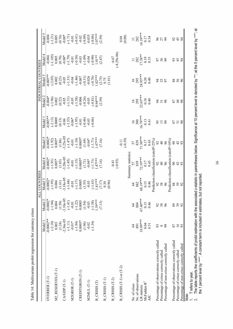
The results for currency crises are reported in Table 14 and Table 15. We include banking crises and a parsimonious set of macroeconomic variables in the regression. A composite crisis dummy that stands for occurrence of banking crisis in either period t-1 or t-2 is included in the explanatory variables. There is evidence that currency crises are preceded by overvaluation of the real exchange rate. Other research has found the real exchange rate to be among the best indicators of currency crises (Goldstein, Kaminsky and Reinhart, 2000). The M2 to foreign reserves ratio is a measure of the central bank’s ability to defend a currency peg when there is adverse foreign exchange speculation. This variable is positively and significantly correlated with currency crises, which means that currency crises are more likely to happen when the central bank does not have sufficient foreign reserves to defend the currency. Current account deficits increase the possibility of a currency crisis. A rapid credit growth tends to precede a currency crisis. In general, these variables are consistent to what the fundamental-based currency crisis models predict (Krugman, 1979, Flood and Garber, 1984). Somehow oddly, we find that a higher M2 to reserve money multiplier is associated with less probability of a currency crisis. Having controlled for the effects of macroeconomic variables, we find that currency crises are significantly correlated with contemporaneous banking crises for all groups of sample. But banking crises occurring within the past year do not help predict the occurrence of currency crises. This is true for all groups of country.8

Multivariate probit regressions for banking crises are reported in Table 16 and Table 17. The probability of a banking crisis generally increases with a slowdown in real growth. Financial 6 Overvaluation of the real exchange rate is calculated as the deviation from the trend specified by the Hodrick-Prescott filter. Increase in the value means real depreciation. 7 The financial liberalization is a dummy variable, which takes the value of one in periods during which interest rates were liberalized. 8 Glick and Hutchison (2001) find that past banking crises help to predict currency crises only in emerging markets.

7

liberalization makes banking crises more likely, although the variable is not significant. Banking crises are correlated with a slowdown of credit growth in the previous year, indicating that a phase of excessive credit expansion might end up well before the crisis broke out.

Again, there is a strong and contemporaneous correlation between banking crises and currency crises. In addition, currency crises occurring within the past year help to predict banking crises for the all countries and developing countries samples. This seems to suggest that, without any implication of causality, twin crises in developing countries tend to show up first as a currency crisis and then followed by a banking crisis. Together with Table 14 and Table 15, there is a symmetric result that banking crises help predict currency crises contemporaneously, and vice versa. This finding is different from Glick and Hutchison (2001), who find significant contemporaneous correlations between banking crises and currency crises only for developing countries and emerging markets, but not for the full sample of countries. In addition, for the samples of all countries and developing countries, there is an asymmetric result in which past currency crises increase the probability of banking crises, but the inverse is not true. This result is opposite to the finding of Kaminsky and Reinhart (1996), who find that past banking crises help predict currency crises, but past currency crises do not help predict banking crises. Glick and Hutchison (2001) likewise find that in none of their samples do past currency crises help to explain banking crises.9

5 Tests of Robustness

The above results are based on banking crises identified using a 2.5% threshold and a 16 quarters window width. We have tried different threshold value (1.5%, 2.5%, and 3.5%) and window widths (12 and 16 quarters) and found most of the above results are robust. Here we summarize briefly the robust test to save space.

The distribution of financial crises over time and the results of signal approach are robust to different specifications. Distribution of financial crises over different groups of countries remains the same. The only finding that requires further qualification is the asymmetric result, which means that past currency crises help predict banking crises, but the converse is not true. One sees that for the samples of all countries and of developing countries, this finding is robust. When a higher threshold is employed and more banking crises are identified, currency and banking crises help to predict each other. This implies that the asymmetric result is sensitive to the number of banking crises identified. However, in no case do we find that banking crises help predict currency crises, but the converse is not true.

6 Conclusion

This paper examines the empirics of twin crises. We treat banking and currency crises equally in terms of identification. We construct an index of money market pressure and an index of foreign currency market pressure to identify banking and currency crises, respectively. Our sample includes 49 countries spanning the period 1980-2001.

Our results display similarities to and show differences with existing research. Most of our findings are robust to different specifications. Our results shed some new light on twin crises. First, earlier research concludes that the frequency of banking crises and twin crises has increased over time. However, we find that banking crises and twin crises were more frequent in the early 1980s. Twin crises are new phenomena and appeared already in the early 1980s. Their frequency declined in mid-1980s but returned to the earlier level in the early 1990s. Second, existing research finds banking crises are good leading indicators of currency crises. We find that although banking crises are more likely to lead than to follow currency crises, but they are good leading indicators of currency crises only for emerging markets. Third, existing research finds an asymmetrical result

9 The correlation between the currency and banking crisis dummies remains the same even if we simply regress the currency crisis dummy on the contemporaneous and lagged banking crisis dummy, and vice versa.

8

between banking and currency crises. It means that past banking crises help to predict currency crises, but the reverse is not true. We also find such an asymmetric character, but its causal direction is just opposite. In other words, we find past currency crises help to predict banking crises, and the converse is not true. Such an asymmetric result is sensitive to the threshold values used in the identification of banking crises.

7 Reference Brüggemann, Axel and Thomas Linne (1999), “How good are Leading Indicators for Currency and Banking

Crises in Central and Eastern Europe? An Empirical Test,” Discussion Papers No. 95/1999, Halle Institute for Economic Research.

Demirgüc-Kunt, Asli and Enrica Detragiache (1998), “The Determinants of Banking Crises in Developing and Developed Countries,” IMF Staff Papers, 45(1), pp.81-109.

Demirgüc-Kunt, Asli and Enrica Detragiache (2000), “Does Deposit Insurance Increase Banking System Stability: An Empirical Investigation,” World Bank Working Papers No. 2247.

Eichengreen Barry, Andrew K. Rose and Charles Wyplosz (1994), “Speculative Attacks on Pegged Exchange Rate: An Empirical Exploration with special Reference to the European Monetary System,” NBER Working Papers No. 4898.

Eichengreen Barry, Andrew K. Rose and Charles Wyplosz (1995), “Exchange Market Mayhem: The Antecedents and Aftermath of Speculative Attacks,” Economic Policy, 21, pp.249-96.

Eichengreen Barry, Andrew K. Rose and Charles Wyplosz (1996), “Contagious Currency Crises,” NBER Working Papers No. 5681.

Eichengreen, Barry and Andrew Rose (1998), “Staying Afloat When the Wind Shifts: External Factors and Emerging-market Banking Crises,” NBER Working Papers No. 6370.

Flood, Robert and P. M. Garber (1984), “Collapsing Exchange-Rate Regimes: Some Linear Examples,” Journal of International Economics, 17, pp.1-13.

Garcia, Gillian G.H. (1999), “Deposit Insurance: A Survey of Actual and Best Practices,” IMF Working Papers No. 99/54.

Glick, Reuven and Michael M. Hutchison (2001), “Banking and Currency Crises: How Common Are Twins?” in Reuven Glick, Ramon Moreno and Mark M. Spiegel (eds.), Financial Crises in Emerging Markets, Cambridge University Press.

Goldstein, Morris, Graciela L. Kaminsky and Carmen M. Reinhart (2000), Assessing Financial Vulnerability: An Early Warning System for Emerging Market, Institute for International Economics.

Kaminsky, Graciela, Saul Lizondo and Carmen M. Reinhart (1998), “Leading Indicators of Currency Crises,” IMF Staff Papers, 45(1), pp.1-48.

Kaminsky, Graciela and Carmen M. Reinhart (1996), “The Twin Crises: The Causes of Banking and Balance-of-Payments Problems,” International Finance Discussion Papers No. 544, Board of Governors of the Federal Reserve System, Washington.

Kaminsky, Graciela and Carmen M. Reinhart (1999), “The Twin Crises: The Causes of Banking and Balance-of-Payments Problems,” American Economic Review, 89(3), pp.473-500.

Krugman, Paul (1979), “A Model of Balance-of-Payments Crises,” Journal of Money, Credit and Banking, 11, pp.311-25.

Rossi, Marco (1999), “Financial Fragility and Economic Performance in Developing Countries,” IMF Working Papers No. 99/66.

Von Hagen, Jürgen and Tai-kuang Ho (2003), “Money Market Pressure and the Determinants of Banking Crises”, mimeo.

Wyplosz, Charles (1999), “The Exchange Rate: Threats and Responses,” in Lorand Ambrus-Lakatos and Mark E. Schaffer (eds.), Monetary and Exchange Rate Policies, EMU and Central and Eastern Europe, CEPR.

9

Ta

ble

1: A

sum

mar

y of

the

findi

ngs o

f exi

stin

g re

sear

ch o

n tw

in c

rises

Stud

y, S

ampl

e,

and

Freq

uenc

y C

ount

ry C

over

age

Met

hodo

logy

Fi

ndin

gs

(1) A

pro

bit m

odel

whe

re th

e cu

rren

cy c

risis

dum

my

is

regr

esse

d ag

ains

t the

ban

king

cris

is d

umm

y, u

nder

al

tern

ativ

e sp

ecifi

catio

ns o

f 12-

mon

th la

g an

d 36

-mon

th la

g an

d a

dum

my

for f

inan

cial

libe

raliz

atio

n. A

sim

ilar p

robi

t m

odel

for b

anki

ng c

rises

.

Ban

king

cris

es a

re si

gnifi

cant

in h

elpi

ng to

pre

dict

cur

renc

y cr

ises

; the

co

nver

se is

not

true

. K

amin

sky

and

Rei

nhar

t (19

96)

1970

to m

id-1

995

Mon

thly

20 c

ount

ries,

incl

udin

g 5

indu

stria

l co

untri

es a

nd 1

5 de

velo

ping

co

untri

es.

(2) F

igur

es p

ortra

ying

the

evol

utio

n of

mac

roec

onom

ic a

nd

finan

cial

var

iabl

es a

roun

d th

e tim

e of

cur

renc

y cr

ises

. Si

mila

r fig

ures

for b

anki

ng c

rises

.

Con

ditio

ns p

rece

ding

the

curr

ency

and

ban

king

cris

es: r

eces

sion

, exp

ort

decl

ine,

hig

h re

al in

tere

st ra

te, f

allin

g st

ock

mar

ket,

and

decl

ine

of te

rms

of tr

ade.

Con

ditio

ns p

rece

ding

cur

renc

y cr

ises

: fal

ling

fore

ign

rese

rves

an

d ra

pid

mon

ey g

row

th. C

redi

t exp

ansi

ons p

reda

te th

e ba

nkin

g cr

ises

. (1

) Fig

ures

por

trayi

ng th

e pr

e-an

d po

st c

rises

beh

avio

r of 1

6 m

acro

econ

omic

and

fina

ncia

l var

iabl

es c

ompa

red

to th

e av

erag

e be

havi

or d

urin

g tra

nqui

l per

iods

, for

cur

renc

y,

bank

ing,

and

twin

cris

es re

spec

tivel

y.

Wea

k an

d de

terio

ratin

g ec

onom

ic fu

ndam

enta

ls ty

pica

lly p

rece

ded

the

twin

cris

es. I

n co

mpa

rison

to c

urre

ncy

or b

anki

ng c

rises

indi

vidu

ally

, ec

onom

ic fu

ndam

enta

ls te

nded

to b

e w

orse

for t

he tw

in c

rises

.

Kam

insk

y an

d R

einh

art (

1999

) 19

70 to

199

5 M

onth

ly

20 c

ount

ries,

incl

udin

g 5

indu

stria

l co

untri

es a

nd 1

5 de

velo

ping

co

untri

es.

(2) S

igna

ls a

ppro

ach

by u

sing

16

indi

cato

rs fo

r cur

renc

y an

d ba

nkin

g cr

ises

resp

ectiv

ely.

B

est l

eadi

ng in

dica

tors

of c

urre

ncy

cris

es: r

eal i

nter

est r

ate,

real

inte

rest

ra

te d

iffer

entia

l, ex

ports

, and

M2

to fo

reig

n re

serv

es ra

tio. B

est l

eadi

ng

indi

cato

rs fo

r ban

king

cris

es: r

eal i

nter

est r

ate,

inte

rest

rate

diff

eren

tial,

term

s of t

rade

, for

eign

rese

rves

, out

put,

expo

rts, a

nd st

ock

pric

es.

(1) S

igna

ls a

ppro

ach:

per

form

ance

of b

ank

cris

es a

s a si

gnal

of

cur

renc

y cr

ises

, and

per

form

ance

of c

urre

ncy

cris

es a

s a

sign

al o

f ban

k cr

ises

.

Ban

king

cris

es te

nd to

be

cont

empo

rane

ous o

r lea

ding

, rat

her t

han

lagg

ing,

indi

cato

rs o

f cur

renc

y cr

ises

.

(2) M

ultiv

aria

te p

robi

t mod

el fo

r cur

renc

y cr

ises

that

incl

ude

the

onse

t of b

anki

ng c

rises

and

a p

arsi

mon

ious

set o

f m

acro

econ

omic

var

iabl

es a

s exp

lana

tory

var

iabl

es.

Lagg

ed a

s wel

l as c

onte

mpo

rane

ous b

ank

cris

es h

elp

to p

redi

ct fu

ture

cu

rren

cy c

rises

in th

e em

ergi

ng m

arke

ts sa

mpl

e. B

ut th

e ba

nk c

risis

va

riabl

e is

not

sign

ifica

nt in

the

deve

lopi

ng c

ount

ry a

nd fu

ll co

untry

sa

mpl

es.

(3) M

ultiv

aria

te p

robi

t mod

el fo

r the

ons

et o

f ban

king

cris

es

that

incl

ude

curr

ency

cris

es a

nd a

par

sim

onio

us se

t of

mac

roec

onom

ic v

aria

bles

as e

xpla

nato

ry v

aria

bles

.

The

onse

t of b

ank

cris

es is

hig

hly

corr

elat

ed w

ith c

otem

pora

neou

s cu

rren

cy c

rises

. But

lagg

ed c

urre

ncy

cris

es a

re n

ot si

gnifi

cant

in

expl

aini

ng th

e on

set o

f ban

k cr

ises

in a

ny o

f the

sam

ples

.

Glic

k an

d H

utch

ison

(200

1)

1975

to 1

997

Ann

ual

90 c

ount

ries,

incl

udin

g 21

in

dust

rial

coun

tries

, 32

emer

ging

mar

kets

, an

d 37

oth

er

deve

lopi

ng

coun

tries

.

(4) S

imul

tane

ous e

quat

ion

prob

it m

odel

for c

urre

ncy

and

bank

ing

cris

es.

Stro

ng c

onte

mpo

rane

ous c

orre

latio

n be

twee

n th

e on

set o

f ban

king

cris

es

and

curr

ency

cris

es in

em

ergi

ng m

arke

ts e

ven

whe

n co

ntro

lling

for

sim

ulta

neou

s bia

s and

oth

er e

xpla

nato

ry v

aria

bles

. How

ever

, no

cont

empo

rane

ous a

ssoc

iatio

n is

seen

in th

e de

velo

ping

cou

ntry

sam

ple

or

in th

e fu

ll gr

oup

of c

ount

ries.

10

Table 2: Countries included in the study and the grouping

Industrial countries Emerging markets Other developing countries Austria Argentina Burundi Denmark Brazil Guatemala Finland Chile Jamaica France Ecuador Nepal Greece Egypt Niger Italy India Senegal Japan Indonesia Togo Netherlands Israel Cyprus Portugal Kenya Swaziland Spain Korea Papua New Guinea Sweden Mexico El Salvador Switzerland Peru Honduras Ireland South Africa Nigeria Germany Sri Lanka Seychelles United States Thailand Uganda New Zealand Turkey Uruguay Venezuela

Number of countries (totally 49 countries) 16 18 15 Note: 1. The “all country” sample includes “industrial countries”, “emerging markets”, and “other developing countries”. The “developing

country” sample includes “emerging markets” as well as “other developing countries”. 2. The classification follows Glick and Hutchison (2001), except for Israel, Niger, Senegal, Togo, Papua New Guinea, and

Seychelles, which are not included in their sample.

Table 3: Occurrences of currency crises: 72 currency crises

THRESHOLD=2 STANDARD DEVIATIONS, WINDOW WIDTH=12 MONTHS Country Currency Crisis Country Currency Crisis Country Currency Crisis Argentina 1982Q3 Israel 1985Q2 Sweden 1992Q3 Argentina 1989Q2 Italy 1981Q2 Switzerland 1981Q3 Brazil 1983Q2 Italy 1992Q3 Switzerland 1989Q1 Brazil 1990Q1 Jamaica 1983Q4 Thailand 1997Q3 Brazil 1999Q1 Jamaica 1992Q1 Togo 1994Q1 Burundi 1992Q2 Japan 1980Q1 Turkey 1994Q2 Burundi 1998Q3 Japan 1990Q2 Turkey 2001Q1 Burundi 2001Q1 Kenya 1993Q3 Uruguay 1982Q4 Chile 1982Q3 Korea 1997Q4 Venezuela 1999Q1 Chile 1984Q4 Mexico 1982Q3 Ireland 1981Q3 Denmark 1980Q1 Mexico 1995Q1 Ireland 1992Q4 Denmark 1982Q4 Nepal 1984Q4 Swaziland 1981Q4 Denmark 2000Q3 Nepal 1991Q3 Swaziland 1985Q1 Ecuador 1986Q3 Netherlands 1981Q3 Germany 1981Q3 Ecuador 1999Q1 Niger 1994Q1 United States 1987Q4 Egypt 1981Q3 Peru 1988Q3 New Zealand 1984Q3 Egypt 1990Q2 Peru 1990Q2 Papua New Guinea 1995Q2 Egypt 1991Q2 Portugal 1983Q3 Papua New Guinea 1998Q1 France 1981Q2 Senegal 1994Q1 El Salvador 1986Q1 Guatemala 1986Q4 South Africa 1982Q1 Honduras 1990Q2 Guatemala 1990Q3 South Africa 1984Q3 Nigeria 1986Q4 India 1991Q3 Spain 1982Q4 Seychelles 1982Q2 Indonesia 1998Q1 Spain 1993Q3 Uganda 1982Q2 Israel 1984Q1 Sril Lanka 1995Q4 Uganda 1989Q1

11

Table 4: Occurrences of banking crises: 63 banking crises

THRESHOLD=2.5%, WINDOW WIDTH=12 QUARTERS Country Banking Crisis Country Banking Crisis Country Banking Crisis Argentina 1989Q2 Jamaica 1993Q1 Spain 1983Q3 Austria 1985Q1 Japan 1985Q4 Spain 1993Q2 Austria 1997Q4 Japan 1998Q3 Sri Lanka 1983Q3 Brazil 1987Q4 Kenya 1993Q1 Sri Lanka 1995Q4 Burundi 1998Q4 Korea 1981Q4 Swaziland 1982Q1 Chile 1984Q2 Korea 1998Q1 Sweden 1992Q3 Cyprus 1982Q4 Mexico 1989Q2 Switzerland 1998Q3 Denmark 1993Q1 Mexico 1995Q2 Thailand 1997Q4 Ecuador 1984Q2 Nepal 1984Q3 Togo 1980Q3 Finland 1989Q4 New Zealand 1983Q1 Togo 1995Q4 France 1981Q3 New Zealand 1988Q2 Turkey 2000Q4 France 1992Q3 Niger 1982Q3 USA 1981Q2 Germany 1980Q3 Nigeria 1989Q4 Uruguay 1982Q4 Germany 1991Q2 Nigeria 1996Q3 Venezuela 1999Q1 Guatemala 1991Q4 Papua New Guinea 1981Q2 Egypt 1990Q4 Guatemala 2001Q2 Peru 1990Q1 El Salvador 1987Q4 India 1984Q2 Portugal 1985Q2 Greece 1991Q4 India 1999Q4 Senegal 1995Q3 Honduras 1985Q1 Indonesia 1998Q1 Seychelles 1982Q1 Ireland 1992Q3 Israel 1984Q3 South Africa 1984Q1 Netherlands 1985Q2 Italy 1992Q2 South Africa 1990Q1 Uganda 1989Q2

Table 5: Occurrence of twin crises, definition 1: 20 twin crises

This study Kaminsky and Reinhart (1999) COUNTRY BANKING CRISIS CURRENCY CRISIS BANKING CRISIS

(onset of) CURRENCY CRISIS

Argentina 1989Q2 1989Q2 March 1980 February 1981 May 1985 September 1986 Chile 1984Q2 1984Q4 September 1981 August 1982 Germany 1980Q3 1981Q3 Indonesia 1998Q1 1998Q1 Israel 1984Q3 1985Q2 October 1983 October 1983 Italy 1992Q2 1992Q3 Kenya 1993Q1 1993Q3 Nepal 1984Q3 1984Q4 New Zealand 1983Q1 1984Q3 Peru 1990Q1 1990Q2 Seychelles 1982Q1 1982Q2 South Africa 1984Q1 1984Q3 Spain 1993Q2 1993Q3 November 1978 December 1982 Sri Lanka 1995Q4 1995Q4 Sweden 1992Q3 1992Q3 November 1991 November 1992 Turkey 2000Q4 2001Q1 January 1991 March 1994 Uruguay 1982Q4 1982Q4 March 1971 December 1971 March 1981 October 1982 Venezuela 1999Q1 1999Q1 October 1993 May 1994 Egypt 1990Q4 1991Q2 Ireland 1992Q3 1992Q4 Note: Definition 1 defines twin crises as episodes in which a banking crisis is followed by a currency crisis within 8 quarters.

12

Table 6: Occurrence of twin crises, definition 2: 28 twin crises

This study Glick and Hutchison (2001) COUNTRY BANKING CRISIS CURRENCY CRISIS BANKING CRISIS CURRENCY CRISISArgentina 1989Q2 1989Q2 1989-1990 1989 Burundi 1998Q4 1998Q3 Chile 1984Q2 1984Q4 France 1981Q3 1981Q2 Germany 1980Q3 1981Q3 Indonesia 1998Q1 1998Q1 1997 1997 Israel 1984Q3 1984Q1, 1985Q2 Italy 1992Q2 1992Q3 Jamaica 1993Q1 1992Q1 Kenya 1993Q1 1993Q3 1985-1989 1985 1992-1997 1993 Korea 1998Q1 1997Q4 1997 1997 Mexico 1995Q2 1995Q1 1981-1991 1982 1995-1997 1994 Nepal 1984Q3 1984Q4 Peru 1990Q1 1990Q2 Seychelles 1982Q1 1982Q2 South Africa 1984Q1 1984Q3 1977 1978 1985 1984 Spain 1983Q3 1982Q4 1977-1985 1976 Spain 1993Q2 1993Q3 Sri Lanka 1995Q4 1995Q4 Swaziland 1982Q1 1981Q4 Sweden 1992Q3 1992Q3 Thailand 1997Q4 1997Q3 1983-1987 1984 1997 1997 Turkey 2000Q4 2001Q1 1994-1995 1994 Uruguay 1982Q4 1982Q4 1981-1984 1982 Venezuela 1999Q1 1999Q1 1994-1997 1994 Egypt 1990Q4 1990Q2, 1991Q2 1980-1985 1979 Ireland 1992Q3 1992Q4 Uganda 1989Q2 1989Q1 Note: Definition 2 defines twin crises as instances in which a banking crisis is accompanied by a currency crisis in either the previous, current, or following year.

Table 7: Distribution of currency and banking crises over time

1980-2001 1980-1984 1985-1989 1990-1994 1995-2001 Banking crises

Number 63 20 13 14 16 Frequency % 5.8 8.2 5.3 5.7 4.7

Currency crises Number 72 27 11 20 14 Frequency % 6.7 11.0 4.5 8.2 4.1

Twin crises (Definition 1) Number 20 8 1 7 4 Frequency % 1.9 3.3 0.4 2.9 1.2

Twin crises (Definition 2) Number 28 10 2 8 8 Frequency % 2.6 4.1 0.8 3.3 2.3 Note: Twin crises in definition 1 are defined as episodes in which a banking crisis is followed by a currency crisis within 8 quarters. Twin crises in definition 2 are defined as instances in which a banking crisis is accompanied by a currency crisis in either the previous, current, or following year (Glick and Hutchison, 2001). Frequency is defined as number of crises divided by total sum of country-years.

13

Table 8: Distribution of currency and banking crises over different groups of countries

Industrial countries Developing countries Emerging markets Banking crises

Number 22 41 23 Frequency % 6.3 5.6 5.8

Currency crises Number 20 52 30 Frequency % 5.7 7.2 7.6

Twin crises (Definition 1) Number 6 14 12 Frequency % 1.7 1.9 3.0

Twin crises (Definition 2) Number 7 21 15 Frequency % 2.0 2.9 3.8 Note: “Developing countries” include “emerging markets” and “other developing countries” as defined in Table 2.

Table 9: Banking crisis as indicator of currency crisis

Signal-to-noise ratio Groups T-4 T-3 T-2 T-1 T T+1 T+2 T+3 T+4 All 1.0 0.9 1.9 7.3 6.2 7.5 4.0 1.0 0.9 Industrial 0.0 3.4 0.0 3.3 3.3 12.1 0.0 0.0 3.5 Developing 1.4 0.0 2.7 9.3 7.6 5.9 5.8 1.4 0.0 Emerging 0.0 0.0 4.8 7.7 14.4 4.9 10.7 2.3 0.0 Note: T refers to quarter. Signal-to-noise ratio is defined as [A/(A+C)]/[B/(B+D)].

Table 10: Banking crisis as indicator of currency crisis, modified

Signal-to-noise ratio Groups T-4 T-3 T-2 T-1 T T+1 T+2 T+3 T+4 All 0.4 0.3 0.3 0.3 0.1 0.3 0.4 0.4 0.4 Industrial 0.2 0.2 0.1 0.1 0.0 0.2 0.2 0.2 0.3 Developing 0.5 0.5 0.5 0.4 0.1 0.3 0.5 0.5 0.5 Emerging 0.8 0.8 0.8 0.5 0.3 0.4 0.9 1.1 1.1 Note: 1. T refers to quarter. 2. Signal-to-noise ratio is defined as A/B. T-N (T+N) refers to signaling window of quarter N after (prior to) the crises.

14

Table 11: Currency crisis as indicator of banking crisis

Signal-to-noise ratio Groups T-4 T-3 T-2 T-1 T T+1 T+2 T+3 T+4 All 0.9 1.0 4.0 7.4 6.1 7.2 1.9 0.9 1.0 Industrial 3.5 0.0 0.0 12.5 3.3 3.3 0.0 3.4 0.0 Developing 0.0 1.4 5.7 5.8 7.4 9.0 2.7 0.0 1.4 Emerging 0.0 2.3 10.2 4.8 13.6 7.5 4.7 0.0 0.0 Note: T refers to quarter. Signal-to-noise ratio is defined as [A/(A+C)]/[B/(B+D)].

Table 12: Currency crisis as indicator of banking crisis, modified

Signal-to-noise ratio Groups T-4 T-3 T-2 T-1 T T+1 T+2 T+3 T+4 All 0.4 0.3 0.3 0.2 0.1 0.2 0.3 0.3 0.3 Industrial 0.3 0.2 0.2 0.2 0.1 0.1 0.1 0.2 0.2 Developing 0.4 0.4 0.3 0.2 0.1 0.3 0.3 0.3 0.4 Emerging 0.7 0.7 0.6 0.3 0.2 0.4 0.5 0.5 0.5 Note: 1. T refers to quarter. 2. Signal-to-noise ratio is defined as A/B. T-N (T+N) refers to signaling window of quarter N after (prior to) the crises.

Table 13: Description of variables and data sources, multivariate probit regression

Variable Name Definition Sources CURRENCY CRISES

OVERRER Overvaluation of real exchange rate (Increase in number means real depreciation)

IFS line RF, line 64, and line 64 of center country. We specify the trend by H-P filter

EXPORTGRO Export growth (in U.S. dollars) IFS line 78AAD M2/RESERVES M2 to foreign reserves ratio M2 from IFS line 34 plus line 35; Foreign reserves

from IFS line 11 (or 1d.d) CA/GDP Current account to GDP ratio Current account from IFS line 78ALD; GDP from

line 99b M2GRON Nominal M2 growth M2 from IFS line 34 plus line 35 M2GROR Real M2 growth M2 from IFS line 34 plus line 35. Then deflated by

line 64 CREDITGRON Nominal credit growth IFS line 32d CREDITGROR Real credit growth IFS line 32d ÷ line 64 M2MUL M2 to reserve money multiplier M2 from IFS line 34 plus line 35; Reserve money

from line 14 (For EURO countries, reserve money is line 14A plus line 14C)

SURPLUS/GDP Budget surplus to GDP ratio Surplus from IFS line 80; GDP from line 99b BANKING CRISES

GROWTH Real GDP growth IFS line 99bvp or 99b.p INFLATION Inflation IFS line 64 FL Dummy for financial liberalization Demirgüc-Kunt and Detragiache (1998), Glick and

Hutchison (2001) CREDITGROR Real credit growth IFS line 32d ÷ line 64 NIRC Nominal interest rate changes Nominal interest rates are from IFS line 60b RIRC Real interest rate changes Nominal interest rates are from IFS line 60b;

Inflation rates are from IFS line 64 SURPLUS/GDP Budget surplus to GDP ratio Surplus from IFS line 80; GDP from line 99b DEPOSITEX Dummy variable for existence of explicit

deposit insurance Garcia (1999), Demirgüc-Kunt and Detragiache (2000)

Note: All variables are compiled from IMF International Financial Statistics, except for FL and DEPOSITEX.

15

Ta

ble

14: M

ultiv

aria

te p

robi

t reg

ress

ion

for c

urre

ncy

cris

es

A

LL C

OU

NTR

IES

IND

UST

RIA

L C

OU

NTR

IES

M

odel

1

Mod

el 2

M

odel

3

Mod

el 4

M

odel

5

Mod

el 1

M

odel

2

Mod

el 3

M

odel

4

Mod

el 5

O

VER

RER

(T-1

) -0

.000

2**

(-2.

10)

-0.0

002*

(-

1.94

) -0

.000

2*

(-1.

95)

-0.0

002*

(-

1.91

) -0

.000

2*

(-1.

92)

-0.0

05**

(-

2.13

) -0

.004

* (-

1.96

) -0

.005

**

(-2.

05)

-0.0

04

(-1.

185)

-0

.004

(-

1.21

) M

2_R

ESER

VES

(T-1

) 0.

003

(1.2

4)

0.00

4 (1

.58)

0.

004

(1.6

1)

0.00

5*

(1.8

3)

0.00

5*

(1.8

6)

0.00

09

(0.1

3)

0.00

2 (0

.22)

0.

002

(0.2

3)

0.00

5 (0

.70)

0.

005

(0.7

6)

CA

/GD

P (T

-1)

-2.3

6e-0

5 (-

1.11

) -3

.10e

-05

(-1.

41)

-3.1

8e-0

5 (-

1.44

) -3

.20e

-05

(-1.

45)

-3.2

5e-0

5 (-

1.47

) -0

.06

(-1.

53)

-0.0

5 (-

1.31

) -0

.05

(-1.

31)

-0.0

8*

(-1.

79)

-0.0

8*

(-1.

71)

M2G

RO

R (T

-1)

-0.0

1*

(-1.

94)

-0.0

1 (-

1.22

) -0

.01

(-1.

17)

-0.0

1 (-

1.15

) -0

.01

(-1.

10)

-0.0

6*

(-1.

95)

-0.0

5 (-

1.58

) -0

.04

(-1.

46)

-0.0

1 (-

0.38

) -0

.01

(-0.

41)

CR

EDIT

GR

ON

(T-1

) 0.

0005

* (1

.96)

0.

0005

(1

.54)

0.

0005

(1

.55)

0.

0005

* (1

.71)

0.

0005

* (1

.69)

-0

.01

(-0.

46)

-0.0

06

(-0.

26)

-0.0

07

(-0.

31)

-0.0

3 (-

1.09

) -0

.02

(-0.

89)

M2M

UL

(T-1

) -0

.02

(-1.

34)

-0.0

3 (-

1.58

) -0

.03

(-1.

63)

-0.0

4*

(-1.

71)

-0.0

4*

(-1.

71)

-0.0

3 (-

0.86

) -0

.03

(-0.

81)

-0.0

26

(-0.

76)

-0.0

4 (-

0.90

) -0

.035

(-

0.86

) B

_CR

ISIS

(T)

1.

39**

* (7

.13)

1.

41**

* (7

.17)

1.

47**

* (7

.16)

1.

47**

* (7

.16)

0.94

***

(2.5

9)

1.02

***

(2.7

5)

1.01

**

(2.4

7)

1.07

***

(2.5

9)

B_C

RIS

IS (T

-1)

0.30

(0

.96)

0.

75(1

.61)

B

_CR

ISIS

(T-2

)

-0.4

1 (-

0.93

) -6

.67

(-8.

29e-

06)

B_C

RIS

IS (T

-1) o

r (T-

2)

-0.1

1 (-

0.39

) 0.

04(0

.08)

Su

mm

ary

stat

istic

s

N

r. of

cris

es64

6464

5757

1616

1611

11N

r. of

obs

erva

tions

89

188

488

283

983

930

029

529

528

228

2LR

stat

istic

18.9

9***

67.4

0***

68.1

9***

72.1

9***

71.3

0***

16.7

9***

22.6

5***

24.9

5***

17.3

8**

16.1

0***

McF

adde

n R

2

0.

040.

150.

150.

170.

170.

130.

180.

200.

190.

17A

IC0.

510.

460.

460.

430.

430.

410.

400.

400.

330.

34Pr

edic

tion

clas

sific

atio

n (c

utof

f=25

%)

Perc

enta

ge o

f obs

erva

tions

cor

rect

ly c

alle

d

9392

9292

9295

9494

9796

Perc

enta

ge o

f cris

es c

orre

ctly

cal

led

838

3840

4013

3125

3627

Perc

enta

ge o

f non

-cris

es c

orre

ctly

cal

led

9996

9696

9699

9897

9999

Pred

ictio

n cl

assi

ficat

ion

(cut

off=

10%

)

Pe

rcen

tage

of o

bser

vatio

ns c

orre

ctly

cal

led

87

8988

9090

8787

8893

92Pe

rcen

tage

of c

rises

cor

rect

ly c

alle

d16

3939

4242

3144

5645

45Pe

rcen

tage

of n

on-c

rises

cor

rect

ly c

alle

d93

9392

9393

9090

9094

94No

te:

1. T

refer

s to y

ear.

2.

The t

able

repo

rts th

e coe

fficien

ts of

prob

it esti

matio

n with

the a

ssoc

iated

z-sta

tistic

in pa

renth

eses

below

. Sign

ifican

ce at

10 pe

rcent

level

is de

noted

by “*

”; at

the 5

perce

nt lev

el by

“**”;

at

the 1

perce

nt lev

el by

“***”

. A co

nstan

t term

is in

clude

d in e

stima

tes, b

ut no

t rep

orted

.

16

Ta

ble

15: M

ultiv

aria

te p

robi

t reg

ress

ion

for c

urre

ncy

cris

es, c

ontin

ue…

D

EVEL

OPI

NG

CO

UN

TRIE

S EM

ERG

ING

MA

RK

ETS

M

odel

1

Mod

el 2

M

odel

3

Mod

el 4

M

odel

5

Mod

el 1

M

odel

2

Mod

el 3

M

odel

4

Mod

el 5

O

VER

RER

(T-1

) -0

.000

2**

(-1.

96)

-0.0

002*

(-

1.79

) -0

.000

2*

(-1.

78)

-0.0

002*

(-

1.76

) -0

.000

2*

(-1.

75)

-0.0

002*

* (-

2.13

) -0

.000

2**

(-1.

99)

-0.0

002*

* (-

2.01

) -0

.000

2**

(-1.

97)

-0.0

002*

* (-

2.00

) M

2_R

ESER

VES

(T-1

) 0.

004

(1.5

7)

0.00

5*

(1.8

5)

0.00

5*

(1.8

5)

0.00

5*

(1.8

5)

0.00

5*

(1.8

4)

0.04

* (1

.94)

0.

03

(1.4

5)

0.03

(1

.45)

0.

03

(1.2

3)

0.03

(1

.26)

C

A/G

DP

(T-1

) -2

.45e

-05

(-1.

13)

-3.2

4e-0

5 (-

1.45

) -3

.21e

-05

(-1.

44)

-3.0

4e-0

5 (-

1.35

) -3

.02e

-05

(-1.

34)

-3.8

0e-0

5 (-

1.52

) -5

.02e

-05*

(-

1.77

) -5

.13e

-05*

(-

1.79

) -4

.95e

-05*

(-

1.72

) -5

.09e

-05*

(-

1.74

) M

2GR

OR

(T-1

) -0

.01

(-1.

59)

-0.0

05

(-0.

90)

-0.0

05

(-0.

91)

-0.0

07

(-1.

22)

-0.0

07

(-1.

22)

-0.0

04

(-0.

72)

-0.0

02

(-0.

37)

-0.0

02

(-0.

36)

-0.0

04

(-0.

64)

-0.0

04

(-0.

60)

CR

EDIT

GR

ON

(T-1

) 0.

0005

* (1

.85)

0.

0004

(1

.36)

0.

0004

(1

.36)

0.

0004

(1

.44)

0.

0004

(1

.43)

0.

0006

**

(2.0

7)

0.00

05

(1.5

9)

0.00

05

(1.6

1)

0.00

05

(1.6

1)

0.00

05

(1.6

0)

M2M

UL

(T-1

) 0.

02

(0.7

3)

0.01

(0

.29)

0.

01

(0.2

9)

0.02

(0

.58)

0.

02

(0.6

0)

-0.0

07

(-0.

17)

-0.0

2 (-

0.41

) -0

.02

(-0.

49)

-0.0

08

(-0.

17)

-0.0

1 (-

0.24

) B

_CR

ISIS

(T)

1.

56**

* (6

.44)

1.

56**

* (6

.40)

1.

63**

* (6

.49)

1.

63**

* (6

.45)

1.89

***

(6.2

3)

1.92

***

(6.2

7)

1.99

***

(6.2

9)

2.02

***

(6.3

4)

B_C

RIS

IS (T

-1)

-0.0

8 (-

0.16

) 0.

51(0

.91)

B

_CR

ISIS

(T-2

)

-0.3

1 (-

0.67

) 0.

14(0

.27)

B_C

RIS

IS (T

-1) o

r (T-

2)

-0.2

1 (-

0.61

) 0.

33(0

.82)

Su

mm

ary

stat

istic

s

N

r. of

cris

es48

4848

4646

2828

2827

27N

r. of

obs

erva

tions

591

589

587

557

557

336

335

335

319

319

LR st

atis

tic

14.9

8**

55.8

3***

55

.72*

**

59.7

0***

59.5

9***

14.0

5**

54.3

355

.08*

**56

.09*

**56

.65*

**M

cFad

den

R2

0.

040.

170.

170.

190.

190.

070.

280.

290.

300.

31A

IC0.

560.

500.

500.

500.

500.

570.

460.

460.

460.

46Pr

edic

tion

clas

sific

atio

n (c

utof

f=25

%)

Perc

enta

ge o

f obs

erva

tions

cor

rect

ly c

alle

d

9292

9292

9291

9292

9292

Perc

enta

ge o

f cris

es c

orre

ctly

cal

led

840

4041

4111

5454

5656

Perc

enta

ge o

f non

-cris

es c

orre

ctly

cal

led

9996

9296

9698

9696

9696

Pred

ictio

n cl

assi

ficat

ion

(cut

off=

10%

)

Pe

rcen

tage

of o

bser

vatio

ns c

orre

ctly

cal

led

83

8988

8989

8090

8990

90Pe

rcen

tage

of c

rises

cor

rect

ly c

alle

d21

4242

4343

3261

6163

59Pe

rcen

tage

of n

on-c

rises

cor

rect

ly c

alle

d88

9293

9493

8493

9293

93No

te:

1. T

refer

s to y

ear.

2. Th

e tab

le re

ports

the c

oeffic

ients

of pr

obit e

stima

tion w

ith th

e ass

ociat

ed z-

statis

tic in

pare

nthes

es be

low. S

ignific

ance

at 10

perce

nt lev

el is

deno

ted by

“*”;

at the

5 pe

rcent

level

by “*

*”; at

the

1 pe

rcent

level

by “*

**”. A

cons

tant te

rm is

inclu

ded i

n esti

mates

, but

not r

epor

ted.

17

Ta

ble

16: M

ultiv

aria

te p

robi

t reg

ress

ion

for b

anki

ng c

rises

A

LL C

OU

NTR

IES

IND

UST

RIA

L C

OU

NTR

IES

M

odel

1

Mod

el 2

M

odel

3

Mod

el 4

M

odel

5

Mod

el 1

M

odel

2

Mod

el 3

M

odel

4

Mod

el 5

G

RO

WTH

(T-1

) -0

.05*

**

(-2.

63)

-0.0

4*

(-1.

73)

-0.0

3 (-

1.45

) -0

.02

(-1.

10)

-0.0

2 (-

0.77

) -0

.09

(-1.

25)

-0.0

8 (-

1.12

) -0

.08

(-1.

12)

-0.0

6 (-

0.75

) -0

.05

(-0.

71)

FL (T

-1)

0.07

(0

.48)

0.

08

(0.5

0)

0.08

(0

.50)

0.

03

(0.2

1)

0.04

(0

.26)

0.

05

(0.1

5)

0.04

(0

.13)

0.

045

(0.1

3)

-0.1

1 (-

0.30

) -0

.09

(-0.

26)

CR

EDIT

GR

OR

(T-1

) -0

.01*

* (-

2.09

) -0

.01*

* (-

2.28

) -0

.01*

* (-

2.01

) -0

.01*

**

(-2.

63)

-0.0

13**

(-

2.32

) -0

.03

(-1.

34)

-0.0

3 (-

1.12

) -0

.03

(-1.

12)

-0.0

3 (-

1.19

) -0

.03

(-1.

19)

C_C

RIS

IS (T

)

1.24

5***

(6

.43)

1.

31**

* (6

.69)

1.

32**

* (6

.52)

1.

35**

* (6

.64)

-0.2

3

-0.0

3

0.92

**(2

.47)

0.

92**

(2

.46)

0.

99**

(2

.34)

0.

98**

(2

.33)

C

_CR

ISIS

(T-1

)

0.

66**

(2

.52)

0.

02(0

.03)

C

_CR

ISIS

(T-2

)

-0.0

6 (-

0.17

) (-

0.37

)

C_C

RIS

IS (T

-1) o

r (T-

2)

0.45

**

(2.0

5)

(-0.

06)

Sum

mar

y st

atis

tics

Nr.

of c

rises

5858

5854

5421

2121

1919

Nr.

of o

bser

vatio

ns

733

732

730

687

687

237

237

237

223

223

LR st

atis

tic17

.02*

**56

.33*

**62

.22*

**56

.32*

**60

.30*

**7.

96**

13.7

1***

13.7

1***

11.6

0***

11.4

6***

McF

adde

nR

2

0.04

0.14

0.15

0.15

0.16

0.06

0.10

0.10

0.09

0.09

AIC

0.54

0.49

0.49

0.49

0.48

0.60

0.58

0.59

0.58

0.59

Pred

ictio

n cl

assi

ficat

ion

(cut

off=

25%

)

Perc

enta

ge o

f obs

erva

tions

cor

rect

ly

calle

d 92

9090

9090

9191

9191

91

Perc

enta

ge o

f cris

es c

orre

ctly

cal

led

235

4035

375

2424

2121

Perc

enta

ge o

f non

-cris

es c

orre

ctly

cal

led

9995

9495

9599

9797

9898

Pred

ictio

n cl

assi

ficat

ion

(cut

off=

10%

)

Perc

enta

ge o

f obs

erva

tions

cor

rect

ly

calle

d 76

8686

8784

6975

7579

80

Perc

enta

ge o

f cris

es c

orre

ctly

cal

led

4843

5244

5067

5757

5353

Perc

enta

ge o

f non

-cris

es c

orre

ctly

cal

led

7990

8890

8769

7676

8282

Note

: 1.

T re

fers t

o yea

r. 2.

The t

able

repo

rts th

e coe

fficien

ts of

prob

it esti

matio

n with

the a

ssoc

iated

z-sta

tistic

in pa

renth

eses

below

. Sign

ifican

ce at

10 pe

rcent

level

is de

noted

by “*

”; at

the 5

perce

nt lev

el by

“**”;

at

the 1

perce

nt lev

el by

“***”

. A co

nstan

t term

is in

clude

d in e

stima

tes, b

ut no

t rep

orted

.

18

Ta

ble

17: M

ultiv

aria

te p

robi

t reg

ress

ion

for b

anki

ng c

rises

, con

tinue

…

D

EVEL

OPI

NG

CO

UN

TRIE

SEM

ERG

ING

MA

RK

ETS

M

odel

1

Mod

el 2

M

odel

3

Mod

el 4

M

odel

5

Mod

el 1

M

odel

2

Mod

el 3

M

odel

4

Mod

el 5

G

RO

WTH

(T-1

) -0

.04*

* (-

2.16

) -0

.02

(-1.

11)

-0.0

2 (-

0.68

) -0

.01

(-0.

53)

-0.0

02

(-0.

10)

-0.0

7***

(-

2.82

) -0

.06*

(-

1.92

) -0

.06*

(-

1.74

) -0

.04

(-1.

38)

-0.0

4 (-

1.17

) FL

(T-1

) 0.

03

(0.1

7)

0.00

8 (0

.04)

-0

.03

(-0.

13)

-0.0

3 (-

0.14

) -0

.049

(-

0.25

) -0

.18

(-0.

75)

-0.2

5 (-

0.95

) -0

.26

(-0.

96)

-0.1

8 (-

0.64

) -0

.19

(-0.

67)

CR

EDIT

GR

OR

(T-1

) -0

.009

* (-

1.72

) -0

.01*

* (-

2.07

) -0

.01*

(-

1.68

) -0

.02*

* (-

2.50

) -0

.01*

* (-

2.02

) 0.

003

(0.4

4)

0.00

07

(0.0

9)

0.00

06

(0.0

7)

-0.0

01

(-0.

12)

-0.0

01

(-0.

16)

C_C

RIS

IS (T

)

1.38

***

(6.0

0)

1.50

***

(6.3

8)

1.46

***

(6.1

6)

1.54

***

(6.3

6)

1.84

***

(6.1

0)

1.85

***

(6.0

7)

1.84

***

(6.0

0)

1.86

***

(6.1

0)

C_C

RIS

IS (T

-1)

0.96

***

(3.1

0)

0.17

(0.3

1)

C_C

RIS

IS (T

-2)

-0

.03

(-0.

08)

0.28

(0.4

7)

C_C

RIS

IS (T

-1) o

r (T-

2)

0.70

***

(2.6

1)

0.29

(0.6

7)

Sum

mar

y st

atis

tics

Nr.

of c

rises

3737

3735

3523

2323

2222

Nr.

of o

bser

vatio

ns

496

495

493

464

464

289

289

289

272

272

LR st

atis

tic11

.30*

**45

.92*

**54

.85*

**48

.17*

**54

.65*

**9.

20**

47.3

5***

47.4

4***

45.9

4***

46.1

7***

McF

adde

n R

2 0.

040.

170.

210.

190.

220.

060.

290.

300.

300.

30A

IC

0.52

0.46

0.45

0.46

0.44

0.55

0.43

0.43

0.44

0.44

Pred

ictio

n cl

assi

ficat

ion

(cut

off=

25%

)

Perc

enta

ge o

f obs

erva

tions

cor

rect

ly

calle

d 92

9189

9190

9193

9393

93

Perc

enta

ge o

f cris

es c

orre

ctly

cal

led

343

4746

494

5757

5959

Perc

enta

ge o

f non

-cris

es c

orre

ctly

cal

led

9995

9394

9499

9696

9696

Pred

ictio

n cl

assi

ficat

ion

(cut

off=

10%

)

Perc

enta

ge o

f obs

erva

tions

cor

rect

ly

calle

d 78

8887

8884

7891

8991

90

Perc

enta

ge o

f cris

es c

orre

ctly

cal

led

4151

5954

6048

6157

5959

Perc

enta

ge o

f non

-cris

es c

orre

ctly

cal

led

8291

8991

8681

9392

9493

Note

: 1.

T re

fers t

o yea

r. 2.

The t

able

repo

rts th

e coe

fficien

ts of

prob

it esti

matio

n with

the a

ssoc

iated

z-sta

tistic

in pa

renth

eses

below

. Sign

ifican

ce at

10 pe

rcent

level

is de

noted

by “*

”; at

the 5

perce

nt lev

el by

“**”;

at

the 1

perce

nt lev

el by

“***”

. A co

nstan

t term

is in

clude

d in e

stima

tes, b

ut no

t rep

orted

.

19

20

Ta

ble

18: S

imul

tane

ous p

robi

t reg

ress

ion

for c

urre

ncy

and

bank

ing

cris

es

A

LL C

OU

NTR

IES

IND

UST

RIA

L C

OU

NTR

IES

DEV

ELO

PIN

G C

OU

NTR

IES

EMER

GIN

G M

AR

KET

S V

aria

bles

C

urre

ncy

cris

is

Ban

king

cris

is

Cur

renc

y cr

isis

B

anki

ng c

risis

C

urre

ncy

cris

is

Ban

king

cris

is

Cur

renc

y cr

isis

B

anki

ng c

risis

O

VER

RER

(T-1

) -0

.000

2**

(-1.

97)

-

005*

*

-00

02*

-

0002

* 0. (-

2.06

) 0. (-

1.84

) 0. (-

1.75

)

M2_

RES

ERV

ES (T

-1)

0.00

3 (1

.35)

0.00

08

0.

005*

0.03

-

06

-

05

-

05

-

06*

-

01

-

002

-

01

0.

0004

0.00

04

-

03

0.

01

-

03

-

25

0.

83

1.

91

-08

-03

-06

**

0.

01

0.

04

-

16

-

03

-

01*

0.

003

0.

44

1.

25

1.

44

of

ises

vatio

ns

**

**

05*

**

* 12

.*

15.

* 10

.*

Fadd

en R

2 04

0.

04

0.06

0.

13

0.05

0.

05

0.08

0.

07

51

0.

59

0.

57

0.53

0.

58

0.55

cal

led

cal

led

cal

led

cal

led

(0.1

1)

(1.6

7)

(1.2

1)

CA

/GD

P (T

-1)

-2.3

1e-0

5 (-

1.08

) 0.

(-1.

53)

2.41

e-(-

1.10

) 3.

66e-

(-1.

47)

M2G

RO

R (T

-1)

-0.0

07

(-1.

18)

0. (-1.

79)

0.(-

0.88

) 0. (-0.

39)

CR

EDIT

GR

ON

(T-1

) 0.

0005

(1

.57)

0.

(-0.

47)

(1.4

5)

(1.2

7)

M2M

UL

(T-1

) -0

.03

(-1.

44)

0.(-

0.86

) (0

.40)

0.

(-0.

65)

B_C

RIS

IS (T

) 0.

79

(0.7

2)

0.(-

0.11

) (0

.73)

(1

.21)

GR

OW

TH (T

-1)

-0

.05*

* (-

2.21

) 0.

(-1.

14)

0.(-

1.45

) 0. (-

2.19

) FL

(T-1

)

0.07

(0

.44)

(0

.03)

(0

.24)

0.

(-0.

66)

CR

EDIT

GR

OR

(T-1

)

-0.0

1**

(-2.

03)

0.(-

1.36

) 0.

(-1.

662)

(0

.45)

C

_CR

ISIS

(T)

0.

47

(0.4

8)

(0.4

1)

(1.0

2)

(1.2

1)

Sum

mar

y st

atis

tics

Nr.

cr63

57

16

20

47

37

28

23

N

r. of

obs

erst

atis

tic

877

730

300

235

577

495

336

289

LR

16.9

5*18

.85*

8.16

.80*

14.8

0*22

*48

*53

*M

c

0.A

IC0.

540.

410.

Pred

ictio

n cl

assi

ficat

ion

(cut

off=

25%

) Pe

rcen

tage

of o

bser

vatio

ns c

orre

ctly

92

93

91

95

92

92

90

91

Perc

enta

ge o

f cris

es c

orre

ctly

cal

led

2 8

5 13

9

3 11

4

Perc

enta

ge o

f non

-cris

es c

orre

ctly

99

99

99

99

99

99

98

99

Pred

ictio

n cl

assi

ficat

ion

(cut

off=

10%

) Pe

rcen

tage

of o

bser

vatio

ns c

orre

ctly

cal

led

78

87

72

87

82

80

80

77

Perc

enta

ge o

f cris

es c

orre

ctly

49

14

60

44

17

38

36

48

Perc

enta

ge o

f non

-cris

es c

orre

ctly

81

93

73

90

87

83

84

79

Note

: 1.

T re

fers t

o yea

r. 2.

The t

able

repo

rts th

e coe

fficien

ts of

prob

it esti

matio

n with

the a

ssoc

iated

z-sta

tistic

in pa

renth

eses

below

. Sign

ifican

ce at

10 pe

rcent

level

is de

noted

by “*

”; at

the 5

perce

nt lev

el by

“**”;

at

the 1

perce

nt lev

el by

“***”

. A co

nstan

t term

is in

clude

d in e

stima

tes, b

ut no

t rep

orted

.