Tutorial: Using SAGA for Least Cost Path...
124
1 Tutorial: Using SAGA for Least Cost Path Analysis Developed by Kim Cimmery (Kapcimmery at hot mail dot com) March 2013 1. Introduction The shortest path between two points is a straight line (unless you are a mariner). The least cost path between two points is the path of least resistance or lowest cost where cost is a function of time or other user-defined factors. In a GIS environment, least cost path analysis is the application of spatial tools to determine the lowest cost path between two or more termination points. Related to the SAGA GIS, here is a reasonable outline for conducting a least cost path analysis in the SAGA environment. 1. Define one or more destination points and one or more source points. 2. Define one or more impact models and cost factors for each that will determine the least cost path solution. 3. Assign a level of importance weight to each cost factor within its’ model. 4. Assign a level of importance weight for each model as part of a composite of models. 5. Define a study area encompassing all destination and source points and a conservative boundary for a spatial solution space. 6. Prepare a grid data layer with data values in grid cells representing destination points. 7. Prepare a point shapes data layer containing point objects representing source points. 8. Develop cost surface grid data layers for each cost factor. 9. Rescale cost surface data layers to a continuous data value range from 0 to 1 using Grid – Calculus/Grid Normalisation, Grid – Calculus/Fuzzify, Grid – Calculus/Grid Calculator, or Grid – Tools/Reclassify Grid Values modules as appropriate. 10. Create a new grid data layer for each cost factor by multiplying the cost surface data layer values by the layers’ importance weight. 11. Develop accumulated cost grid data layers for each cost factor using the Grid – Analysis/Accumulated Cost (Isotropic) module. 12. Develop a least cost path for each factor (or combination of factors if models are used) using the Grid – Analysis/Least Cost Paths module. 13. Apply evaluation criteria and compare least cost path solutions. This outline basically summarizes the approach I use in this tutorial. Least cost path analysis (LCPA) is used to identify and evaluate the least cost path solution for a (hypothetical) proposed power line corridor between two existing electric power substations. Rather than using multiple destination or multiple source points, this analysis
Transcript of Tutorial: Using SAGA for Least Cost Path...

1
Tutorial: Using SAGA for Least Cost Path Analysis
Developed by Kim Cimmery
(Kapcimmery at hot mail dot com)
March 2013
1. Introduction
The shortest path between two points is a straight line (unless you are a mariner). The
least cost path between two points is the path of least resistance or lowest cost where cost
is a function of time or other user-defined factors. In a GIS environment, least cost path
analysis is the application of spatial tools to determine the lowest cost path between two
or more termination points.
Related to the SAGA GIS, here is a reasonable outline for conducting a least cost path
analysis in the SAGA environment.
1. Define one or more destination points and one or more source points.
2. Define one or more impact models and cost factors for each that will determine
the least cost path solution.
3. Assign a level of importance weight to each cost factor within its’ model.
4. Assign a level of importance weight for each model as part of a composite of
models.
5. Define a study area encompassing all destination and source points and a
conservative boundary for a spatial solution space.
6. Prepare a grid data layer with data values in grid cells representing destination
points.
7. Prepare a point shapes data layer containing point objects representing source
points.
8. Develop cost surface grid data layers for each cost factor.
9. Rescale cost surface data layers to a continuous data value range from 0 to 1 using
Grid – Calculus/Grid Normalisation, Grid – Calculus/Fuzzify, Grid –
Calculus/Grid Calculator, or Grid – Tools/Reclassify Grid Values modules as
appropriate.
10. Create a new grid data layer for each cost factor by multiplying the cost surface
data layer values by the layers’ importance weight.
11. Develop accumulated cost grid data layers for each cost factor using the Grid –
Analysis/Accumulated Cost (Isotropic) module.
12. Develop a least cost path for each factor (or combination of factors if models are
used) using the Grid – Analysis/Least Cost Paths module.
13. Apply evaluation criteria and compare least cost path solutions.
This outline basically summarizes the approach I use in this tutorial. Least cost path
analysis (LCPA) is used to identify and evaluate the least cost path solution for a
(hypothetical) proposed power line corridor between two existing electric power
substations. Rather than using multiple destination or multiple source points, this analysis
2
involves two terminal points, each being a substation. The northern substation is referred
to as the destination and the southern substation referred to as the source. This is
terminology implemented in two key SAGA modules for least cost path analysis: Grid –
Analysis/Accumulated Cost (Isotropic) and Grid – Analysis/Least Cost Paths.
I have three models that I call determinant models. Each model describes a cost or impact
theme that determines a least cost path solution between the two substations. Within each
model are factor elements that are weighted for overall importance relative to the other
factor elements in the model. The step before applying the importance weights is to
rescale the factor element data values to the continuous data value range from 0 to 1, with
1 representing the highest cost. Once factor element layers are rescaled, the importance
weights are applied to each data value in the grid layer. The weighted factor element
layers are combined into a single cost surface layer. I am using a set of weights as a
given. How they were generated is not part of the tutorial.
The cost surface layer for the model along with a grid data layer for the destination
substation are inputs to the Grid – Analysis/Accumulated Cost (Isotropic) module. The
output grid data layer from this module has values representing the accumulated cost
radiating out from the location of the destination substation. The grid cell position for the
destination substation on the accumulated cost layer has a data value of 0. The further a
grid cell is from the destination substation, the more cost is accumulated for the cell from
the cost surface layer.
The accumulated cost grid data layer and the point shapes data layer for the source
substation are inputs to the Grid – Analysis/Least Cost Paths module. The module
explores all combinations of cost values starting from the source substation and going to
the destination substation location on the accumulated cost layer seeking the combination
with the lowest total cost. The combination of grid cells having the lowest cost represent
the least cost path solution. Each of the three determinant models has a least cost path
solution.
After developing the individual model solutions, I use two sets of weights for combining
the model cost surface layers into composite solutions. One set of weights represents each
model having equal weight. A second set varies the importance weights for the models.
Using the model importance weights, the models are combined to develop a solution
based on equal importance of each model and a second solution where one perspective is
significantly more important than the other two.
The last section of the tutorial provides an example for using evaluation criteria to
compare the impacts for the five least cost path solutions. A 600-foot wide corridor (300
feet on either side of the line) is created for each least cost path solution. The evaluation
criteria involve number of residences per corridor, comparing corridor estimated market
value, comparing differences in south-facing slopes and slope gradient, and changes in
land use class acres between corridors.

3
Most of the sections in the tutorial include an overview near the beginning of the section
followed by a more detailed description. The overview is a brief outline of the processing
steps that are expanded in the description section.
This tutorial is a logical extension of the tutorial on the application of multi-criteria
evaluation techniques. These techniques were explored in the “Multi_Criteria
Evaluation_Tutorial” that can be downloaded from the SAGA website “Tutorial” section.
It is not necessary to be familiar with MCE techniques to use this tutorial but familiarity
would enhance the experience.
Development of this tutorial was supported with the 64-bit version of SAGA 2.1.0. Prior
to the release of 2.1.0, monthly builds with the latest developments are available in the
files repository (https://sourceforge.net/projects/saga-gis/files/SAGA%20-
%202.0/SAGA%202.1%20Bets/).
As you go through this tutorial, if you encounter mistakes please let me know. My e-mail
contact address is kapcimmery at hotmail dot com.
Scenario
A local public utility department (PUD), as part of its’ strategic planning process,
proposes a new 115 KV transmission line between two existing sub-stations. The PUD
wants to use GIS technology to explore potential corridor locations related to three
viewpoints. They describe these viewpoints as human health, landscape, and nature. In
addition, they want to develop potential corridor locations by merging the models into
two composites using two different sets of importance weights.
Figure 1-1 displays the study area location in eastern Mason County, Washington state,
USA. One of the substations is located to the north of the southern portion of the Hood
Canal and the other substation is located in the southwest quadrant near the town of
Shelton. The straight-line distance between the two points is about 14 miles.

4
Figure 1-1. The study area source and destination substation locations.
I have created a grid system encompassing the study area displayed in Figure 1-1. The
grid system is: “60; 1623x 1926y; 973100.585936x 690802.630098y”. The “60” defines
the grid cell size as 60 feet by 60 feet. The grid system is rectangular in shape and made
up of 1623 columns and 1926 rows of grid cells. Notice that the study area boundary,
displayed with the thick black line in the figure, is not rectangular but has an irregular
shape. There are many instances in this tutorial where a module produces data values for
the small area within the rectangular shape of the grid system that is in fact outside of the
study area. You will see that when data values occur outside of the study area I go
through a process to convert the values to no data values.
The human health determinant model has three factor elements. The density of residential
structures is used as a proxy for population. Distance away from residential structures is a
second element. Schools are interpreted as sensitive buildings. Distance from sensitive
buildings is the third factor element for the model.
The landscape determinant model has two distance related factor elements: distance away
from highly valued cultural and recreation sites and distance from sensitive non-
residential buildings. Recreation sites include county, non-county, and community parks.

5
Cultural sites are public libraries. Sensitive non-residential buildings include buildings
used for commercial and industrial purposes. In addition, there are factor elements for
visibility from these sites and buildings.
Four factor elements make up the nature determinant model. South-oriented slope aspects
are considered critical wildlife areas because of their use by important bird species and
the presence of upward air currents. Road buffers for federal, state and local roads will be
calculated and distance from these corridors calculated. A third factor element is land
cover based on the degree of natural vegetation cover. Land cover is assigned a value
from low to high depending on whether it is agriculture, forest, open space, etc. The risk
for bird collision with transmission facilities is higher around ridges. Buffers are defined
for ridges. The buffer width depends on the elevation of the ridge. Distance from the
ridge buffers is then calculated.
The three models described above are similar to models that were used in an
environmental impact assessment project a couple years ago in Italy (see reference for
Bagli, et al in the reference section of this tutorial). The names of the models do not, in
my opinion, adequately describe the model. Based on the factor elements of the models,
however, I could not come up with more appropriate terms. The models will be referred
to, in general, as human health, landscape, and natural throughout this tutorial.
The Mason County GIS Group, located in Shelton, Washington, distributes a CD
containing many of the layers making up the County ESRI ARC-INFO GIS database.
Most of the layers provide county coverage. These layers are the source of much of the
data used in this tutorial.
SAGA Modules Used in the Tutorial
Grid – Analysis/Least Cost Paths
Grid – Analysis/Accumulated Cost (Isotropic)
Grid – Calculus/Fuzzify
Grid – Calculus/Grid Normalisation
Grid – Calculus/Grid Calculator
Grid – Gridding/Shapes to Grid
Grid – Gridding/Kernel Density Estimation
Grid – Tools/Grid Buffer
Grid – Tools/Grid Masking
Grid – Tools/Proximity Grid
Grid – Tools/Reclassify Grid Values
Grid – Tools/Threshold Buffer
Shapes - Tools/Copy Selection to New Shapes Layer
Shapes – Tools/Create New Shapes Layer
Shapes - Tools/Merge Shapes Layers
Shapes - Tools/Select by Attributes … (Numerical Expression)
Spatial and Geostatistics – Grids/Zonal Grid Statistics
Table – Calculus/Table Calculator (Shapes)
Terrain Analysis – Lighting, Visibility/Visibility (single point) [interactive]

6
Terrain Analysis – Morphometry/Slope, Aspect, Curvature
Terrain Analysis – TPI Based Landform Classification
2. The Human Health Determinant Model.
The human health determinant model has these three factor elements:
Density of Residential Structures (.50)
Distance from Residential Structures (.25)
Distance from Sensitive Buildings (.25)
The values in parentheses for the factor elements are importance weights used when the
layers are aggregated to create a cost surface grid data layer for the model. The first
element has an importance weight of .50 that indicates that the element is twice as
important as the other two elements as they each have an importance weight of .25.
Notice that the total for all three weights is 1.
This model indirectly considers negative health effects from transmission lines. The less
population near a transmission line the lower the overall impact on people. The more
distant a line is from residential structures and sensitive buildings the lower the impact. A
corollary to these statements is that the closer a transmission line is to residential
structures, sensitive buildings, and high population density areas, the higher the potential
impact.
Density of Residential Structures
Overview
1. Execute the Kernel Density Estimation module; the ‘LcaSiteAddresses’ point
layer is the input layer. The default output ‘LcaSiteAddresses [Kernel Density]’
layer contains density values and uses 0 values for no data values.
2. Change the no data value on the ‘LcaSiteAddresses [Kernel Density]’ layer from
0 to –99999 using the ‘No Data’ parameter in the ‘Settings’ tab in the ‘Object
Properties’ window. Save the layer as ‘LcaPopEstTEMPGR’. The 0 data values
occurring outside of the study area boundary need to be converted to no data
values of –99999.
3. Execute the Grid Masking module; the ‘LcaPopEstTEMPGR’ layer is input and
the grid data layer for the study area (‘LcaStudyAreaGR’) is a second input. The
default output grid data layer is ‘Masked Grid’. It is renamed
‘LcaPopEstimateGR’. Grid cells within the study area contain valid data values
including 0’s and grid cells outside of the study area contain no data values of –
99999.
4. Rescale the data range on the ‘LcaPopEstimateGR’ layer to the continuous data
range from 0 to 1 using the Grid Normalisation module. Areas with no population
will have 0 values. As population density increases, data values increase from 0 to
a maximum of 1. The default output grid ‘Normalised Grid’ is renamed
‘LcaPopEstimateGRNM’.
7
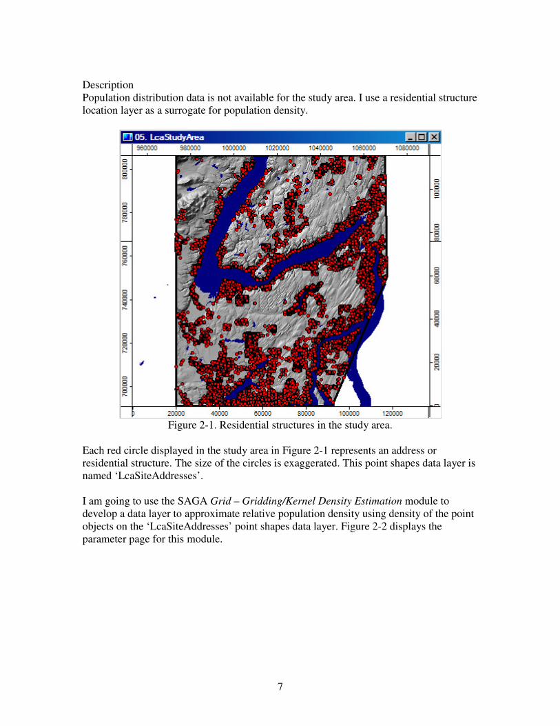
Description
Population distribution data is not available for the study area. I use a residential structure
location layer as a surrogate for population density.
Figure 2-1. Residential structures in the study area.
Each red circle displayed in the study area in Figure 2-1 represents an address or
residential structure. The size of the circles is exaggerated. This point shapes data layer is
named ‘LcaSiteAddresses’.
I am going to use the SAGA Grid – Gridding/Kernel Density Estimation module to
develop a data layer to approximate relative population density using density of the point
objects on the ‘LcaSiteAddresses’ point shapes data layer. Figure 2-2 displays the
parameter page for this module.

8
Figure 2-2. The Kernel Density Estimation module parameter page.
The ‘LcaSiteAddresses’ point shapes data layer is chosen for the ‘>>Points’ input
parameter. The “ID2” attribute is selected to represent the ‘Population’ parameter. The
“ID2” attribute for each point in the layer has the value 1. In the ‘Options’ section, a
radius of 1000 is entered, the “gaussian kernel” option chosen for the ‘Kernel’ parameter
and “grid” is chosen for the ‘Target Grid’ parameter. The two ‘Kernel’ parameter options
“gaussian” and “quartic” are variations for smoothing data. I am not sure exactly when I
would use one over the other but my understanding is that the “guassian” kernel option is
used most often. The radius value is in feet and can affect the number of residences used
in the calculations and the resulting density value. The larger the radius the higher the
potential of more residence points being used. The data values on the output layer for this
module will be rescaled to a continuous data range from 0 to 1. My interest in the values
is in their relative value and not in their absolute value. I click the ‘Okay’ button and the
module executes.
The default output from the Kernel Density Estimation module is the grid data layer
‘LcaSiteAddresses [Kernel Density]’. The data storage type for this output layer is “4
byte floating point number”. Normally, the no data value would be –99999. However,
possibly because 0 is not a valid density value, the module set a different no data value
for the storage type rather than use the default. The no data value used is 0.0. In this
tutorial, for this particular data layer, I consider 0 to be a valid data value.
I can easily change the ‘No Data’ value parameter in the ‘Settings’ tab area in the ‘Object
Properties’ window for the ‘LcaSiteAddresses [Kernel Density]’ grid data layer. See
Figure 2-3. I make the ‘LcaSiteAddresses [Kernel Density]’ layer active by moving the
mouse pointer over the layer name appearing in the ‘Data’ tab area of the Workspace and
press the left mouse button. I click the ‘Settings’ tab in the ‘Object Properties’ window
and the parameter information for the layer displays. Toward the top of the display is a
parameter named ‘No Data’. I change the 0; 0 that appears in the value field to –99999; -

9
99999 by retyping the values or I could click on the plus symbol to the left of the
parameter and enter –99999 for both the ‘Minimum’ and ‘Maximum’ parameters. This
means that any occurrence of 0 is now interpreted as a valid data value and that any
occurrence of –99999 is now treated as the no data value. Keep in mind that the layer
does not yet contain any values of –99999.
Figure 2-3 displays the upper portion of the ‘Settings’ tab before and after making this
change.
Figure 2-3. The ‘No Data’ parameter in the ‘Settings’ tab area.
After making this change, I move the mouse pointer back over the layer name
‘LcaSiteAddresses [Kernel Density]’ in the ‘Data’ tab area of the Workspace, press the
right mouse button, and choose the ‘Save As’ option from the pop-up list of options. I
then save the changed layer as ‘LcaPopEstTEMPGR’.
I have converted the 0 no data values to valid 0 data values by changing the ‘No Data’
parameter in the ‘Settings’ tab area for the layer ‘Object Properties’ from 0; 0 to –99999;
-99999. When I do this, however, an unwanted result is that grid cells outside of the study
area but still within the grid system now contain the valid data value 0.
As a reminder, a SAGA grid system is rectangular in shape and cannot be an irregular
outline. The study area has an irregular shape with the southeast corner of the SAGA grid
system being outside of the study area. I use the Grid Masking module to convert the 0
values outside of the study area to no data values using –99999 for the no data value.
The Grid – Tools/Grid Masking module uses two input layers. One is a layer that
contains the grid cell definition for the study area. This layer serves as a mask. On this
layer, each cell that is within the study area contains the data value 1 and cells outside of
the study area the no data value -99999. The name of this layer is ‘LcaStudyAreaGR’.
This layer was created using the Grid – Gridding/Shapes to Grid module to convert a

10
polygon shapes data layer of the study area boundary (‘LcaStudyArea’). When the
‘LcaStudyAreaGR’ layer is used in the module as the ‘>>Mask’ grid, cells on the second
input (‘>>Grid’) that are outside of the study area boundary are assigned a no data value,
in this case –99999.
The parameter page for the Grid – Tools/Grid Masking module is displayed in Figure 2-
4.
Figure 2-4. The parameter page for the Grid Tools – Grid Masking module.
The ‘LcaPopEstTEMPGR’ grid data layer is chosen for the input parameter ‘>>Grid’.
The “[create]” option is chosen for the output ‘<Masked Grid’ parameter. The grid data
layer ‘LcaStudyAreaGR’ is entered for the ‘>>Mask’ input parameter. I move the mouse
pointer to the ‘Okay’ button, click the left mouse button, and the module executes.
The output grid data layer is named ‘Masked Grid’. I rename it to ‘LcaPopEstimateGR’
and save it.
The data range for the ‘LcaPopEstimateGR’ layer is 0 to 125.200325. You can determine
the data range for a layer by checking in the ‘Settings’ tab area of the ‘Object Properties’
window when the layer is made active. The parameter field ‘Value Range’ displays the
range in the ‘Minimum’ and ‘Maximum’ parameters. The data range can also be
determined by viewing the ‘Description’ tab area.
On the ‘LcaPopEstimateGR’ layer, values greater than 0 indicate presence of population.
The intent is to develop a factor element cost layer that contains data values rescaled into
continuous values between 0 and 1 for the for the continuous data range from 0 to
125.200325. Because impacts are higher in more densely populated areas, the range from
0 to 1 stands for impacts from low to high.
The Grid – Calculus/Grid Normalisation module is used to rescale the data values on the
‘LcaPopEstimateGR’ layer. Figure 2-5 displays the parameter page for this module.

11
Figure 2-5. The Grid – Calculus/Grid Normalisation module parameter page.
The ‘LcaPopEstimateGR’ grid data layer is chosen for the ‘>>Grid’ parameter and
“[create]” is used for the output ‘<<Normalised Grid’ parameter. The data range of the
input grid data layer is rescaled to continuous values between 0 and 1. The minimum and
maximum values are entered for the ‘Target Range’ parameter. I click the ‘Okay’ button
and the module executes.
Note that the Grid – Calculus/Grid Normalisation module rescaling capability is flexible.
The minimum and maximum values entered for the ‘Target Range’ parameter could
define a data range for any set of continuous values; e.g., 0 to 255 or 1 to 0. In fact we
will rescale data values for several factor elements where the existing data range of
continuous values is inversely rescaled to values between 1 and 0.
The output grid data layer ‘Normalised Grid’ is renamed to ‘LcaPopEstimateGRNM’ and
saved.
The data values on the ‘LcaPopEstimateGRNM’ layer range from 0 to 1 and stand for an
increasing range of impact, 1 being the highest level where the population density is
highest and 0 for the absence of population.
This last step, to normalize the data range for the factor element grid data layer, is
common to all of the factor elements for all three models. As you would expect, the
various layers exhibit unique data ranges. It is necessary to adjust the different data
ranges scales before combining the layers using the weights such that they all use a
common numeric scale. The varying data ranges are all rescaled to a range of continuous
values between 0 and 1.
12
Distance From Residential Structures
Overview
1. Convert the ‘LcaSiteAddresses’ point shapes layer to a grid data layer using the
Grid-Gridding/Shapes to Grid module. Rename the default output grid data layer
‘LcaSiteAddresses [ID]’ to ‘LcaSiteAddressesGR’.
2. Use the grid layer ‘LcaSiteAddressesGR’ as input to the Grid-Tools/Proximity
Grid module to produce a layer with grid cells of distances from features to cells
containing no data values. The default output layer is named ‘Distance’.
3. Use the ‘Distance’ layer as input for the Grid-Tools/Grid Masking module to
recode data values outside of the study area to no data values (-99999). Rename
the default output layer ‘Masked Grid’ to ‘LcaAddressDistGR’.
4. Rescale the data range of distance values on the ‘LcaAddressDistGR’ layer to a 0
to 1 range with the Grid – Calculus/Grid Normalisation module. Rename the
default output layer ‘Normalised Grid’ to ‘‘LcaAddressDistGRNM’.
Description
The Euclidian distance to no data grid cells from map features (e.g., buildings) can be
calculated with the SAGA Grid-Tools/Proximity Grid module. The input layer for this
module is a grid data layer where grid cell values define the location of features. On this
grid layer, features will have data values and all other cells will contain the no data value.
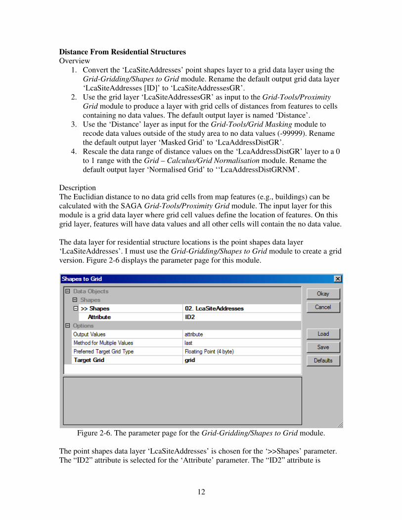
The data layer for residential structure locations is the point shapes data layer
‘LcaSiteAddresses’. I must use the Grid-Gridding/Shapes to Grid module to create a grid
version. Figure 2-6 displays the parameter page for this module.
Figure 2-6. The parameter page for the Grid-Gridding/Shapes to Grid module.
The point shapes data layer ‘LcaSiteAddresses’ is chosen for the ‘>>Shapes’ parameter.
The “ID2” attribute is selected for the ‘Attribute’ parameter. The “ID2” attribute is
13
populated with 1’s for all the point objects in the layer. The “grid” option is chosen for
the ‘Target Grid’ parameter. I click the ‘Okay’ button and the module executes.
A dialog window opens at the start of execution requesting a grid system be identified. In
order for the study area grid system to be available as a choice, at least one grid data layer
that is a part of the study area grid system must be loaded for the work session. The study
area grid system is chosen for this parameter and “[create]” for the ‘<<Grid’ parameter.
Other modules used in this tutorial have the same parameter requirement, ‘Grid system’,
e.g., the next one that is discussed, the Grid-Tools/Proximity Grid module. Most of the
time you will already have loaded a grid data layer that is part of the study area grid
system.
The default output grid is named ‘LcaSiteAddresses [ID2]’. I rename the output layer to
‘LcaSiteAddressesGR’ and save it.
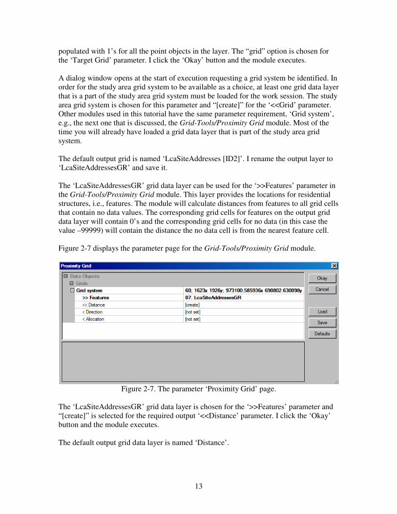
The ‘LcaSiteAddressesGR’ grid data layer can be used for the ‘>>Features’ parameter in
the Grid-Tools/Proximity Grid module. This layer provides the locations for residential
structures, i.e., features. The module will calculate distances from features to all grid cells
that contain no data values. The corresponding grid cells for features on the output grid
data layer will contain 0’s and the corresponding grid cells for no data (in this case the
value –99999) will contain the distance the no data cell is from the nearest feature cell.
Figure 2-7 displays the parameter page for the Grid-Tools/Proximity Grid module.
Figure 2-7. The parameter ‘Proximity Grid’ page.
The ‘LcaSiteAddressesGR’ grid data layer is chosen for the ‘>>Features’ parameter and
“[create]” is selected for the required output ‘<<Distance’ parameter. I click the ‘Okay’
button and the module executes.
The default output grid data layer is named ‘Distance’.
14
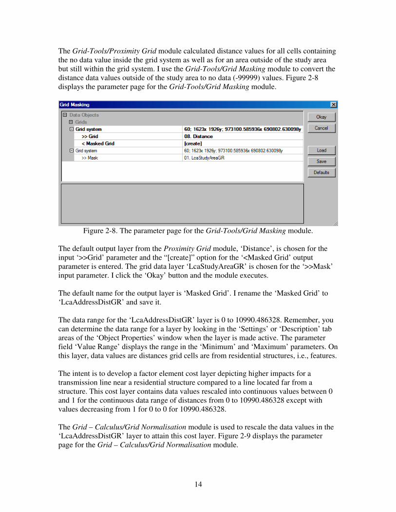
The Grid-Tools/Proximity Grid module calculated distance values for all cells containing
the no data value inside the grid system as well as for an area outside of the study area
but still within the grid system. I use the Grid-Tools/Grid Masking module to convert the
distance data values outside of the study area to no data (-99999) values. Figure 2-8
displays the parameter page for the Grid-Tools/Grid Masking module.
Figure 2-8. The parameter page for the Grid-Tools/Grid Masking module.
The default output layer from the Proximity Grid module, ‘Distance’, is chosen for the
input ‘>>Grid’ parameter and the “[create]” option for the ‘<Masked Grid’ output
parameter is entered. The grid data layer ‘LcaStudyAreaGR’ is chosen for the ‘>>Mask’
input parameter. I click the ‘Okay’ button and the module executes.
The default name for the output layer is ‘Masked Grid’. I rename the ‘Masked Grid’ to
‘LcaAddressDistGR’ and save it.
The data range for the ‘LcaAddressDistGR’ layer is 0 to 10990.486328. Remember, you
can determine the data range for a layer by looking in the ‘Settings’ or ‘Description’ tab
areas of the ‘Object Properties’ window when the layer is made active. The parameter
field ‘Value Range’ displays the range in the ‘Minimum’ and ‘Maximum’ parameters. On
this layer, data values are distances grid cells are from residential structures, i.e., features.
The intent is to develop a factor element cost layer depicting higher impacts for a
transmission line near a residential structure compared to a line located far from a
structure. This cost layer contains data values rescaled into continuous values between 0
and 1 for the continuous data range of distances from 0 to 10990.486328 except with
values decreasing from 1 for 0 to 0 for 10990.486328.
The Grid – Calculus/Grid Normalisation module is used to rescale the data values in the
‘LcaAddressDistGR’ layer to attain this cost layer. Figure 2-9 displays the parameter
page for the Grid – Calculus/Grid Normalisation module.

15
Figure 2-9. The Grid – Calculus/Grid Normalisation module parameter.
The ‘LcaAddressDistGR’ grid data layer is chosen for the input ‘>>Grid’ parameter and
“[create]” for the output ‘<<Normalised Grid’ parameter. The data range of distances on
the input grid data layer is rescaled to continuous values between 0 and 1. The minimum
and maximum values are entered for the ‘Target Range’ parameter. Setting the
‘Minimum’ parameter to 1 means that the value 1 is used for the rescale of the lowest
value of the data range of the input layer, 0. Using 0 for the ‘Maximum’ parameter means
that the value 0 is used for the rescale of the highest value of the input layer,
10990.486328. The values between 0 and 10990.486328 are rescaled decreasing between
1 and 0. I click the ‘Okay’ button and the module executes.
The output grid data layer ‘Normalised Grid’ is renamed ‘LcaAddressDistGRNM’ and
saved.
The data values on the ‘LcaAddressDistGRNM’ layer range from 0 to 1 and define an
increasing range of impact, 1 being the highest level for cells adjacent to residential
structures and 0 for cells the most distant from residential structures. Cells in between
have continuous data values increasing from 0 to 1. You will note that this is one of the
factor elements where the existing data range of continuous values is inversely rescaled
to values between 0 and 1.
Distance From Sensitive Buildings
Overview
1. Convert the ‘LcaSchools’ point shapes layer to a grid data layer using the Grid-
Gridding/Shapes to Grid module. Rename the default output grid data layer
‘LcaSchools [ID]’ to ‘LcaSchoolsGR’.
2. Use the grid layer ‘LcaSchoolsGR’ as input to the Grid-Tools/Proximity Grid
module to produce a layer containing distance values in cells representing the
distance the no data cell is from the nearest feature. The default output grid data
layer is called ‘Distance’.
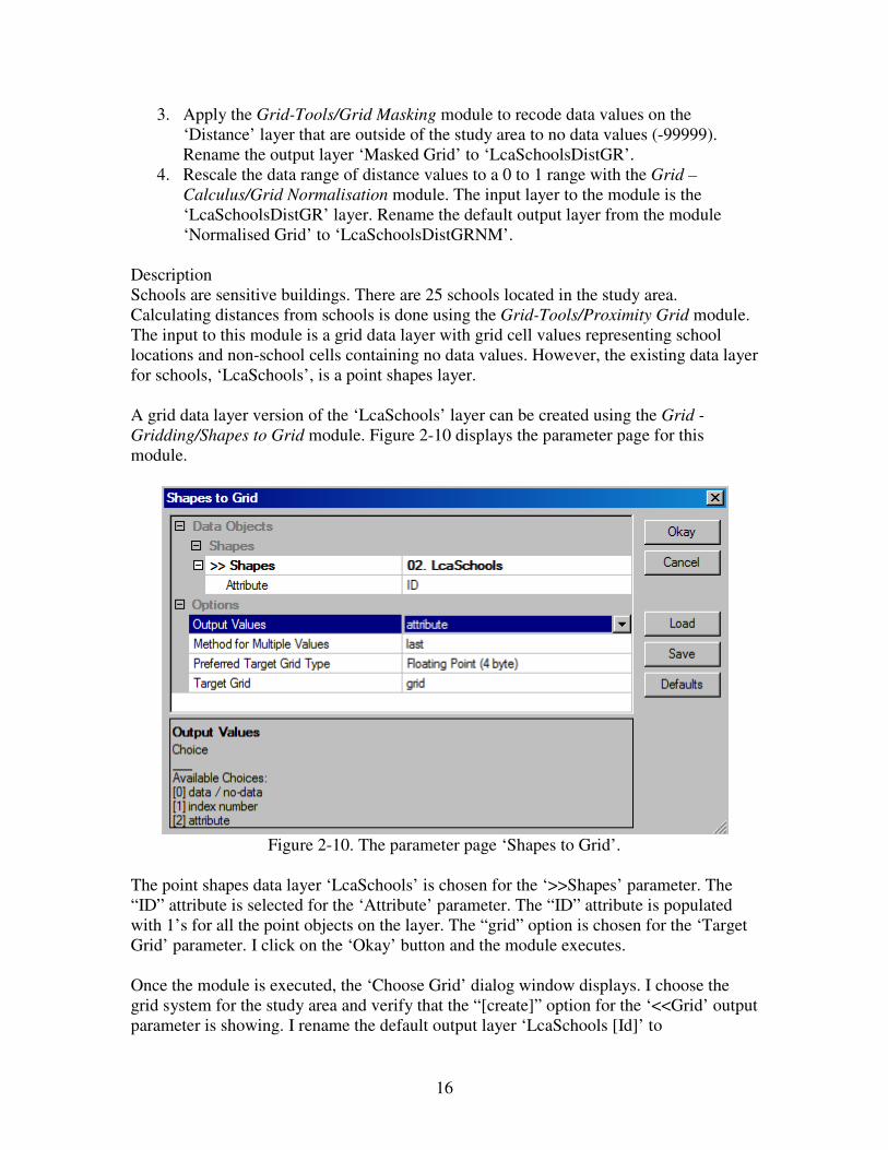
16
3. Apply the Grid-Tools/Grid Masking module to recode data values on the
‘Distance’ layer that are outside of the study area to no data values (-99999).
Rename the output layer ‘Masked Grid’ to ‘LcaSchoolsDistGR’.
4. Rescale the data range of distance values to a 0 to 1 range with the Grid –
Calculus/Grid Normalisation module. The input layer to the module is the
‘LcaSchoolsDistGR’ layer. Rename the default output layer from the module
‘Normalised Grid’ to ‘LcaSchoolsDistGRNM’.
Description
Schools are sensitive buildings. There are 25 schools located in the study area.
Calculating distances from schools is done using the Grid-Tools/Proximity Grid module.
The input to this module is a grid data layer with grid cell values representing school
locations and non-school cells containing no data values. However, the existing data layer
for schools, ‘LcaSchools’, is a point shapes layer.
A grid data layer version of the ‘LcaSchools’ layer can be created using the Grid -
Gridding/Shapes to Grid module. Figure 2-10 displays the parameter page for this
module.
Figure 2-10. The parameter page ‘Shapes to Grid’.
The point shapes data layer ‘LcaSchools’ is chosen for the ‘>>Shapes’ parameter. The
“ID” attribute is selected for the ‘Attribute’ parameter. The “ID” attribute is populated
with 1’s for all the point objects on the layer. The “grid” option is chosen for the ‘Target
Grid’ parameter. I click on the ‘Okay’ button and the module executes.
Once the module is executed, the ‘Choose Grid’ dialog window displays. I choose the
grid system for the study area and verify that the “[create]” option for the ‘<<Grid’ output
parameter is showing. I rename the default output layer ‘LcaSchools [Id]’ to
17
‘LcaSchoolsGR’ and save it. On this layer, grid cells identifying school locations contain
data values and all non-school cells contain the no data value –99999.
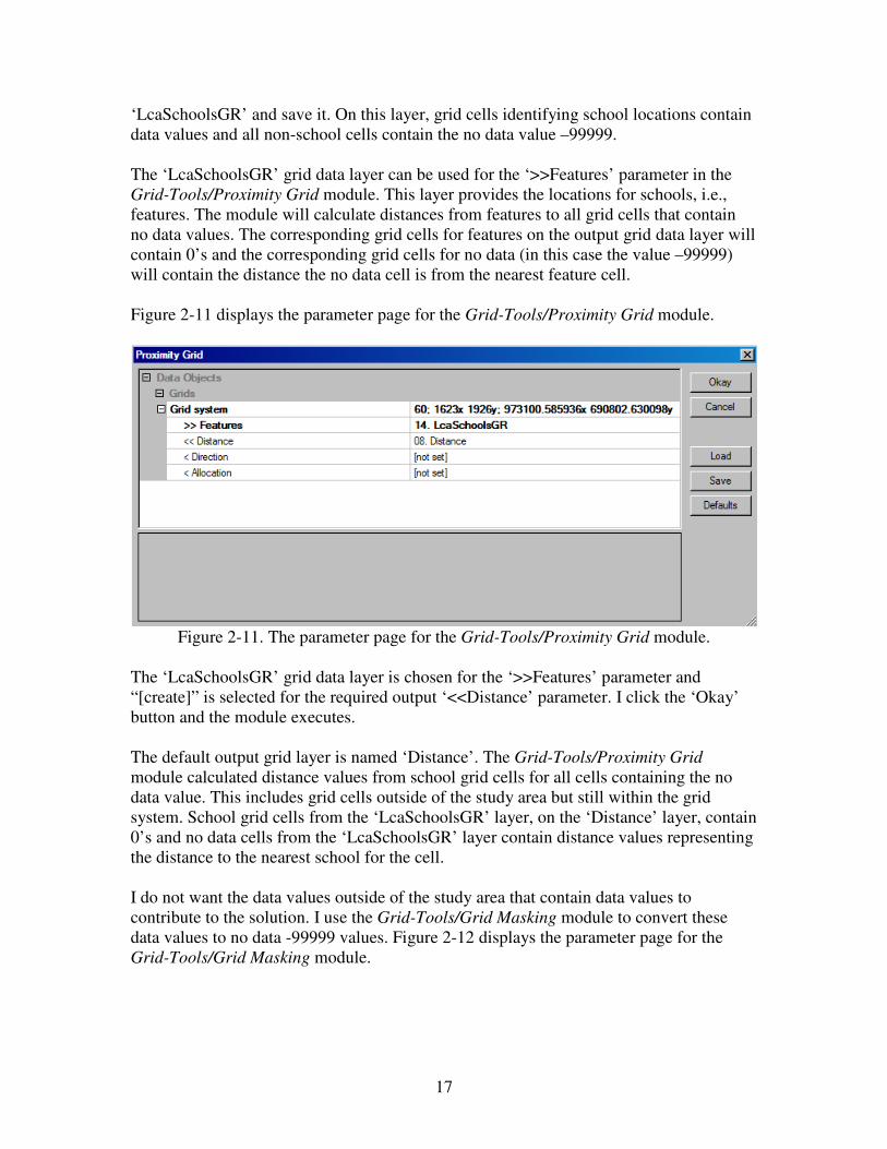
The ‘LcaSchoolsGR’ grid data layer can be used for the ‘>>Features’ parameter in the
Grid-Tools/Proximity Grid module. This layer provides the locations for schools, i.e.,
features. The module will calculate distances from features to all grid cells that contain
no data values. The corresponding grid cells for features on the output grid data layer will
contain 0’s and the corresponding grid cells for no data (in this case the value –99999)
will contain the distance the no data cell is from the nearest feature cell.
Figure 2-11 displays the parameter page for the Grid-Tools/Proximity Grid module.
Figure 2-11. The parameter page for the Grid-Tools/Proximity Grid module.
The ‘LcaSchoolsGR’ grid data layer is chosen for the ‘>>Features’ parameter and
“[create]” is selected for the required output ‘<<Distance’ parameter. I click the ‘Okay’
button and the module executes.
The default output grid layer is named ‘Distance’. The Grid-Tools/Proximity Grid
module calculated distance values from school grid cells for all cells containing the no
data value. This includes grid cells outside of the study area but still within the grid
system. School grid cells from the ‘LcaSchoolsGR’ layer, on the ‘Distance’ layer, contain
0’s and no data cells from the ‘LcaSchoolsGR’ layer contain distance values representing
the distance to the nearest school for the cell.
I do not want the data values outside of the study area that contain data values to
contribute to the solution. I use the Grid-Tools/Grid Masking module to convert these
data values to no data -99999 values. Figure 2-12 displays the parameter page for the
Grid-Tools/Grid Masking module.
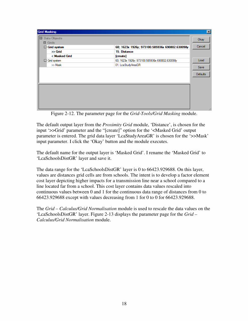
18
Figure 2-12. The parameter page for the Grid-Tools/Grid Masking module.
The default output layer from the Proximity Grid module, ‘Distance’, is chosen for the
input ‘>>Grid’ parameter and the “[create]” option for the ‘<Masked Grid’ output
parameter is entered. The grid data layer ‘LcaStudyAreaGR’ is chosen for the ‘>>Mask’
input parameter. I click the ‘Okay’ button and the module executes.
The default name for the output layer is ‘Masked Grid’. I rename the ‘Masked Grid’ to
‘LcaSchoolsDistGR’ layer and save it.
The data range for the ‘LcaSchoolsDistGR’ layer is 0 to 66423.929688. On this layer,
values are distances grid cells are from schools. The intent is to develop a factor element
cost layer depicting higher impacts for a transmission line near a school compared to a
line located far from a school. This cost layer contains data values rescaled into
continuous values between 0 and 1 for the continuous data range of distances from 0 to
66423.929688 except with values decreasing from 1 for 0 to 0 for 66423.929688.
The Grid – Calculus/Grid Normalisation module is used to rescale the data values on the
‘LcaSchoolsDistGR’ layer. Figure 2-13 displays the parameter page for the Grid –
Calculus/Grid Normalisation module.

19
Figure 2-13. The Grid – Calculus/ Grid Normalisation module parameter page.
The ‘LcaSchoolsDistGR’ grid data layer is chosen for the input ‘>>Grid’ parameter and
“[create]” for the output ‘<<Normalised Grid’ parameter. The data range of distances on
the input grid data layer is rescaled to continuous values between 0 and 1. The minimum
and maximum values are entered for the ‘Target Range’ parameter. Setting the
‘Minimum’ parameter to 1 means that the value 1 is used for the rescale of the lowest
value of the data range of the input layer, 0. Using 0 for the ‘Maximum’ parameter means
that the value 0 is used for the rescale of the highest value of the input layer,
66423.929688. The values between 0 and 66423.929688 are rescaled decreasing between
1 and 0. I click the ‘Okay’ button and the module executes.
The output grid data layer ‘Normalised Grid’ is renamed ‘LcaSchoolsDistGRNM’ and
saved.
The data values on the ‘LcaSchoolsDistGRNM’ layer range from 0 to 1 and stand for an
increasing range of impact, 1 being the highest level for cells adjacent to schools and 0
for cells the most distant from schools. Cells in between have continuous data values
increasing from 0 to 1. You will note that this is one of the factor elements where the
existing data range of continuous values is inversely rescaled to values between 0 and 1.
The Human Health Model Least Cost Path
Overview
1. Apply the importance weight to each factor element grid data layer and combine the
weighted factor element layers into a single cost surface layer using the Grid –
Calculus/Grid Calculator module. Name the combined layer ‘LcaCostHthModGR’.
2. Use the aggregate factor element cost surface layer (‘LcaCostHthModGR’) for the
model and the grid data layer for the destination substation (‘LcaDestinationPointGR’) as
inputs to the Grid – Analysis/Accumulated Cost (Isotropic) module and create the
accumulated cost grid data layer. Name the accumulated cost grid data layer
‘LcaAccumHthModGR’.
20
3. The point shapes data layer for the source substation (‘LcaSourcePoint’) and the
accumulated cost grid data layer, ‘LcaAccumHthModGR’, are inputs to the Grid –
Analysis/Least Cost Paths module for calculating the least cost path solution for the
model. The default shapes outputs ‘Profile_Line_[LcaAccumHthModGR]_1’) and
‘Profile_Points_[LcaAccumHthModGR]_1’ are renamed to ‘LcaLCPAlineMod1’ and
‘LcaLCPApointsMod1’.
Description
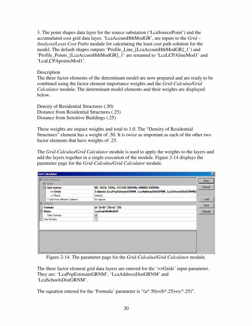
The three factor elements of the determinant model are now prepared and are ready to be
combined using the factor element importance weights and the Grid-Calculus/Grid
Calculator module. The determinant model elements and their weights are displayed
below.
Density of Residential Structures (.50)
Distance from Residential Structures (.25)
Distance from Sensitive Buildings (.25)
These weights are impact weights and total to 1.0. The “Density of Residential
Structures” element has a weight of .50. It is twice as important as each of the other two
factor elements that have weights of .25.
The Grid-Calculus/Grid Calculator module is used to apply the weights to the layers and
add the layers together in a single execution of the module. Figure 2-14 displays the
parameter page for the Grid-Calculus/Grid Calculator module.
Figure 2-14. The parameter page for the Grid-Calculus/Grid Calculator module.
The three factor element grid data layers are entered for the ‘>>Grids’ input parameter.
They are: ‘LcaPopEstimateGRNM’, ‘LcaAddressDistGRNM’ and
‘LcaSchoolsDistGRNM’.
The equation entered for the ‘Formula’ parameter is “(a*.50)+(b*.25)+(c*.25)”.
21
The variables a, b, and c in the equation represent the three grid data layers in the input
parameter value field in the order they appear. The values .50, .25 and .25 are the
importance weights. The weight for a layer will multiply the data values in the layer grid
cells, e.g., “a*.50”. The products for corresponding grid cells are added together (e.g.,
“(a*.50)+(b*.25)+…”) and output to the corresponding grid cell of the output grid data
layer named ‘LcaCostHthModGR’. This is the cost surface layer for the model.
The cost surface layer (‘LcaCostHthModGR’) and the ‘LcaDestinationPointGR’ layer are
the input layers to the Grid – Analysis/Accumulated Cost (Isotropic) module. The default
output layer ‘Accumulated Cost’ from this module contains cumulative cost data values
radiating out from the single destination point grid cell on the ‘LcaDestinationPointGR’
layer. The more distant a grid cell is from the cell with the zero value (the destination
point) the more cost is accumulated in the cell. Figure 2-15 displays the parameter page
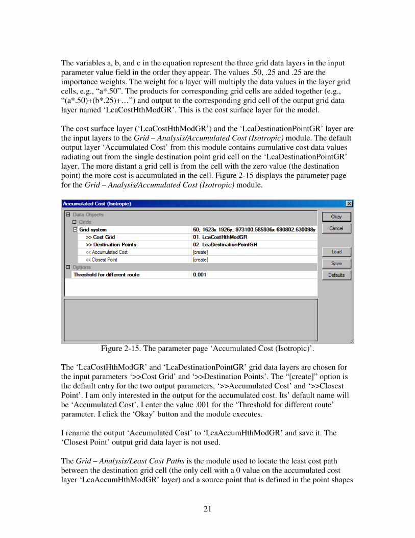
for the Grid – Analysis/Accumulated Cost (Isotropic) module.
Figure 2-15. The parameter page ‘Accumulated Cost (Isotropic)’.
The ‘LcaCostHthModGR’ and ‘LcaDestinationPointGR’ grid data layers are chosen for
the input parameters ‘>>Cost Grid’ and ‘>>Destination Points’. The “[create]” option is
the default entry for the two output parameters, ‘>>Accumulated Cost’ and ‘>>Closest
Point’. I am only interested in the output for the accumulated cost. Its’ default name will
be ‘Accumulated Cost’. I enter the value .001 for the ‘Threshold for different route’
parameter. I click the ‘Okay’ button and the module executes.
I rename the output ‘Accumulated Cost’ to ‘LcaAccumHthModGR’ and save it. The
‘Closest Point’ output grid data layer is not used.
The Grid – Analysis/Least Cost Paths is the module used to locate the least cost path
between the destination grid cell (the only cell with a 0 value on the accumulated cost
layer ‘LcaAccumHthModGR’ layer) and a source point that is defined in the point shapes

22
data layer named ‘LcaSourcePoint’. The destination point is the substation located in the
northern half of the study area and the source point is the station in the southwest
quadrant of the study area. Figure 2-16 displays the parameter page for the Grid –
Analysis/Least Cost Paths module.
Figure 2-16. The parameter page for the Grid – Analysis/Least Cost Paths module.
The grid data layer ‘LcaAccumHthModGR’ is chosen for the ‘>>Accumulated cost’
parameter. This is the output layer from the Grid – Analysis/Accumulated Cost
(Isotropic) module. The point shapes data layer ‘LcaSourcePoint’ is chosen for the
‘>>Source Point(s)’ input parameter. This layer contains the point object for the
substation located in the southwest quadrant of the study area. I click on the ‘Okay’
button and the module executes.
The Grid – Analysis/Least Cost Paths module produces two shapes layers; one is a line
shapes data layer (default name ‘Profile_Line_[LcaAccumHthModGR]_1’) and the other
is a point shapes data layer (default name ‘Profile_Points_[LcaAccumHthModGR]_1’).
The point shapes data layer has point objects defining the location of the least cost path
between the two points. A point object is defined for each grid cell the least cost path
solution traverses. The line shapes data layer is a line defining the location of the least
cost path between the two points. I rename the default output layers to
‘LcaLCPApointsMod1’ and ‘LcaLCPAlineMod1’ and save both of them.
The default line shapes data layer output contains a single line object. The attribute table
has a single attribute named “ID” and the default value for the “ID” attribute is 1.
The default point shapes data layer contains a point object for every grid cell the least
cost line solution traverses starting with the source terminal point. The attribute table
linked to the point shapes data layer has five attributes. Figure 2-17 displays a portion of
a sample attribute table.

23
Figure 2-17. A portion of the ‘Profile_Points_[LcaAccumHthModGR]_1’ attribute table.
Each point object has a unique “ID” starting with 1. The first point identifies the location
of the source point. The last “ID” used is for the location of the destination point, in this
case, the location of the northern substation. The “ID” for this last point is 1128. This
means that the line traverses 1128 grid cells.
The “D” attribute is the cumulative distance from one grid cell to the next starting at the
source point and increasing to the destination point. The grid cells are 60’ by 60’ square.
The least cost path solution line can move in one of 8 directions between cells; it can
move horizontal or vertical (4 directions) or it can move diagonal from each corner (4
directions). The distance between cells moving horizontal or vertical, center-to-center, is
60’. The distance moving diagonally is 84.852814’. The distance between point object 1
and point object 2 (see Figure 2-17) is 84.852814’. This means the least cost path
solution is exiting from the first cell (the source point) in a diagonal direction. The value
for the “D” attribute for the last point object in the table is also the total distance in feet
for the line.
24
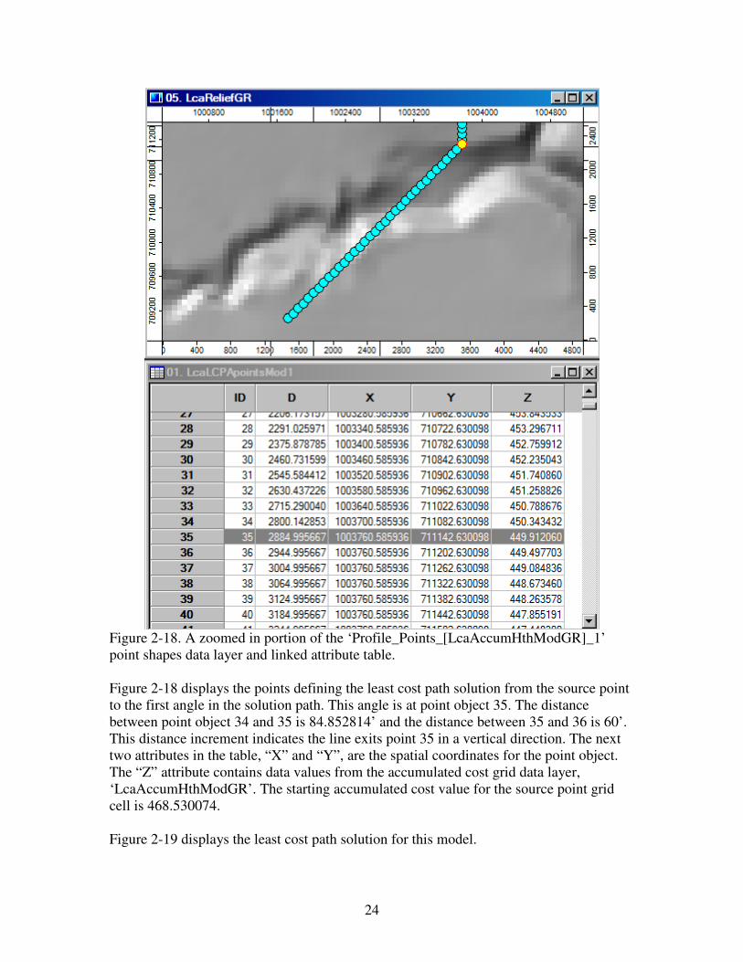
Figure 2-18. A zoomed in portion of the ‘Profile_Points_[LcaAccumHthModGR]_1’
point shapes data layer and linked attribute table.
Figure 2-18 displays the points defining the least cost path solution from the source point
to the first angle in the solution path. This angle is at point object 35. The distance
between point object 34 and 35 is 84.852814’ and the distance between 35 and 36 is 60’.
This distance increment indicates the line exits point 35 in a vertical direction. The next
two attributes in the table, “X” and “Y”, are the spatial coordinates for the point object.
The “Z” attribute contains data values from the accumulated cost grid data layer,
‘LcaAccumHthModGR’. The starting accumulated cost value for the source point grid
cell is 468.530074.
Figure 2-19 displays the least cost path solution for this model.

25
Figure 2-19. The least cost path solution for the human health determinant model.
The two substations are displayed using small red circles in Figure 2-19. The substation
to the north of the large body of water (the south end of Hood Canal) is the destination.
The substation in the southwest quadrant of the display is the source. The green line
connecting the two substations is the least cost path solution for the human health
determinant model. The road network for the study area is displayed in black and the
background is the topographic relief in shades of gray. Water areas are filled with blue.
There is an optional output parameter for the Grid – Analysis/Least Cost Paths module
that I am not using. It is named ‘>Values’ (see Figure 2-16). Related to this, there is a
SAGA module named Shapes – Grids/Add Grid Values to Points. This module allows
you to include grid cell values from existing grid data layers as attributes and attribute
values for point objects. The capability of the Shapes – Grids/Add Grid Values to Points
module is integrated into the Grid – Analysis/Least Cost Paths module through the
‘>Values’ parameter. As an example, I choose the ‘LcaDEMfeetGR’ layer for the
‘>Values’ parameter (the parameter supports multiple layers). This layer contains
elevation data values for the study area.
Figure 2-20 displays a portion of the attribute table for the output point shapes data layer
generated from executing the Grid – Analysis/Least Cost Paths module with the
‘LcaDEMfeetGR’ layer identified for the ‘>Values’ parameter.

26
Figure 2-20. A zoomed in portion of a sample attribute table showing the
“LcaDEMfeetGR” attribute field.
A new attribute appears following the “Z” attribute named “LcaDEMfeetGR” for the
study area DEM layer. The values in this attribute are elevation values.
Figure 2-21. A sample profile using the “LcaDEMfeetGR” attribute.
The profile displayed in Figure 2-21 was created by moving the mouse pointer over the
point shapes data layer name in the ‘Data’ tab area of the Workspace. I pressed the right
mouse button, moved the mouse to the ‘Attributes’ option, and chose the ‘Diagram’
command and chose the “LcaDEMfeetGR” attribute for the basis of the diagram.
27
3. The Landscape Determinant Model.
The landscape model has four factor elements.
Distance From Highly Valued Cultural and Recreational Sites (.10)
Visibility From Highly Valued Cultural and Recreational Sites (.45)
Distance From Sensitive Non-Residential Buildings (.10)
Visibility From Sensitive Non-Residential Buildings (.35)
The values in parentheses for the factor elements are the importance weights used when
the layers are aggregated to create the cost surface for the model. Thus, you can see that
the “Visibility From Highly Valued Cultural and Recreational Sites” and “Visibility
From Sensitive Non-Residential Buildings” factor elements each have a higher
importance in the model than the other two factor elements. These two elements will
have a significant influence on the data values for the cost surface layer. The remaining
two elements account for 20 percent of the model.
This model relates to two types of cultural features: cultural and recreational sites and
sensitive non-residential buildings. Cultural and recreational sites are defined as county
and non-county parks and public libraries. Commercial and industrial buildings are going
to be used for sensitive non-residential buildings. The closer a transmission corridor is to
these categories of sites, the higher the impact and the more visible a transmission
corridor is from these sites, the higher the impact.
Distance From Highly Valued Cultural and Recreational Sites
Overview
1. Select the four community parks in the ‘LcaSiteAddresses’ layer using the
Shapes-Tools/Select by Attributes … (Numerical Expression) module and create a
new layer containing only the four parks with the Shapes-Tools/Copy Selection to
New Shapes Layer module. This new layer is named ‘LcaCommParks’.
2. Merge the four layers containing point objects for county and non-county parks
and libraries into a single point shapes data layer using the Shapes-Tools/Merge
Shapes Layers module. Save it as ‘LcaParksLibs’.
3. Add the new “SITE” attribute to the parks and library shapes data layer. Resave
the ‘LcaParksLibs’ layer.
4. Convert the ‘LcaParksLibs’ shapes layer to a grid data layer using the Grid-
Gridding/Shapes to Grid module. Name the new grid layer ‘LcaParksLibsGR’.
5. Use the grid layer ‘LcaParksLibsGR’ as input to the Grid-Tools/Proximity Grid
module to produce a layer containing cells with distances from features values.
The default output grid data layer for the Proximity Grid module is named
‘Distance’.
6. Use the ‘Distance’ layer as input to the Grid-Tools/Grid Masking module and
recode data values outside of the study area to no data values (-99999). Rename
the default output layer ‘Masked Grid’ to ‘LcaParksLibsDistGR’.
7. Rescale the data range of distance values to a 0 to 1 range on the
‘LcaParksLibsDistGR’ layer with the Grid – Calculus/Grid Normalisation
module. Rename the default output layer ‘Normalised Grid’ to
‘LcaParksLibsDistGRNM’.

28
Description
“Highly Valued Cultural and Recreational Sites” are defined in this tutorial as county
parks, non-county parks and libraries.
Point shapes data layers named ‘LcaCountyParks’ and ‘LcaNon-CountyParks’ exist for
county and non-county recreational sites. However, there are four community parks not
included on these layers that are point objects on the ‘LcaSiteAddresses’ point shapes
data layer. Prior to dealing with the first two factor elements of this model, I want to
develop a single point shapes data layer containing points for county and non-county
parks, community parks, and libraries.
There is a layer, ‘LcaLibraries’, for libraries in the study area.
I need to “select” the four community parks (points) in the ‘LcaSiteAddresses’ point
shapes data layer and copy the selected points to a new shapes data layer. I will use the
Shapes-Tools/Select by Attributes … (Numerical Expression) module to select the point
objects.
The attribute table linked to the ‘LcaSiteAddresses’ layer has an attribute named “ID” in
which the four community parks point records contain the value 4. They are the only
records in the table with the value 4 for the “ID” attribute. Figure 3-1 displays the
parameter page for the Shapes-Tools/Select by Attributes … (Numerical Expression)
module.
Figure 3-1. The Shapes-Tools/Select by Attributes … (Numerical Expression) module
parameter page.
The ‘LcaSiteAddresses’ point shapes data layer is chosen for the input parameter
‘>>Shapes’. The “ID” attribute is selected for the ‘Attribute’ parameter. The equation

29
“a=4” is entered for the ‘Expression’ parameter. The letter “a” is a variable representing
the “ID” attribute. The value to be searched for is 4 and the method will be “new
selection”. This is a simple selection. Other selection options for the ‘Method’ parameter
are “add to current selection”, “select from current selection”, and “remove from current
selection”. I click on the ‘Okay’ button and the module executes.
Figure 3-2 displays the portion of the ‘LcaSiteAddresses’ layer where the four
community parks are located. The four point objects are highlighted in yellow as a result
of the above selection process by the Shapes-Tools/Select by Attributes … (Numerical
Expression) module.

30
Figure 3-2. Results from the Shapes-Tools/Select by Attributes … (Numerical Expression)
module.
The lower part of Figure 3-2 is a portion (8 records) of the attribute table. When the
module selects records they become selected and highlighted in the attribute table. When
the attribute table is displayed in a table view window, you can right click with the mouse
in the far left column to see a set of options. One of the options is “Sort Selection to
Top”. You can see that I chose that option. The four community park highlighted records
are displayed as the first four records of the table.
31
I use the Shapes-Tools/Copy Selection to New Shapes Layer module to copy the four
selected points (and records attribute data) to a new point shapes data layer. I rename the
new layer ‘LcaCommParks’ and save it.
The Shapes-Tools/Merge Shapes Layers module is used to merge the ‘LcaCountyParks’,
‘LcaNon-CountyParks’, ‘LcaLibraries’, and the new layer ‘LacCommParks’ into a new
point shapes data layer that is to be named ‘LcaParksLibs’. The parameter page for the
Shapes-Tools/Merge Shapes Layers module is displayed in Figure 3-3.
Figure 3-3. The Shapes-Tools/Merge Shapes Layers module parameter page.
The output parameter, ‘<<Merged Layer’, has the “[create]” option chosen. The default
name for the output layer is ‘Shapes_Merge’. The structure of the attribute table for the
shapes data layer chosen for the ‘>>Main Layer’ parameter will be the structure of the
attribute table for the output shapes layer ‘Shapes_Merge’. This will be the table structure
regardless of the structures of the attribute tables for the layer or layers identified for the
‘>Additional Layers’ parameter.
Three of the four layers being merged have the same attribute table structure. The fourth
one, the ‘LcaCommParks’ layer, has the field structure copied from the
‘LcaSiteAddresses’ layer. I have chosen to use the ‘LcaLibraries’ layer for the ‘>>Main
Layer’ parameter. The other three layers are chosen for the ‘>Additional Layers’
parameter. I click on the ‘Okay’ button to execute the module with these parameters.
The default output point shapes data layer contains 40 point objects. I rename the output
point shapes data layer ‘Shapes_Merge’ to ‘LcaParksLibs’ and save it.
I should note that I am not too concerned about which attribute table structure is used.
However, I do want to add an attribute that I will name “SITE” to the attribute table. This
new attribute will contain a unique number for each of the 40 point objects. This attribute
field will be used later during on-screen digitizing of observer points and delineating
viewsheds for the sites.
I add the new attribute “SITE” by first displaying the attribute table for the merged layers
‘LcaParksLibs’ point shapes data layer. I display the table by right clicking with the

32
mouse on the point shapes data layer name in the ‘Data’ tab section of the Workspace.
When the pop-up menu of options appears, I move the mouse pointer to the “Attributes”
option toward the bottom of the list. Another pop-up menu appears and I choose the
“Show” option.
When the table displays, I move the mouse pointer into the top row of the table where the
attribute names display and click the right mouse button. I choose the “Add Field” option
from the pop-up list and follow the directions for defining a new field. In the ‘Name’
parameter field I enter “SITE”. I choose the “2 byte integer” option for the ‘Field Type’
parameter and identify the “ID” field for the ‘Insert Position’ parameter and “After” for
the ‘Insert Method’.
Once the above definition process is finished, I click the ‘Okay’ button and the new field
appears in the table. Starting with the first record, I click and enter a 1, the second record
I enter a 2, and so on until I have entered 40 for the last record. I save the new version of
the table and my entries by right-clicking on the file name in the ‘Data’ tab area and
choose the “Save” option in the pop-up menu.
There are 40 point objects in the ‘LcaParksLibs’ layer. Each point will be treated the
same in this model regardless of whether the point represents a park or a library. The first
step to incorporate this element into the model is to create a grid version of the point
shapes data layer ‘LcaParksLibs’.
The Grid-Tools/Proximity Grid module is going to be used for distance calculations. The
input layer for this module is a grid data layer. Before I can calculate distances from
parks and libraries, I need to create a grid data layer version of the point shapes data layer
‘LcaParksLibs’. The grid data layer version will be used as input to the Grid-
Tools/Proximity Grid module.
I use the Grid-Gridding/Shapes to Grid module to develop a grid version of the point
shapes layer ‘LcaParksLibs’. Figure 3-4 displays the parameter page for this module.
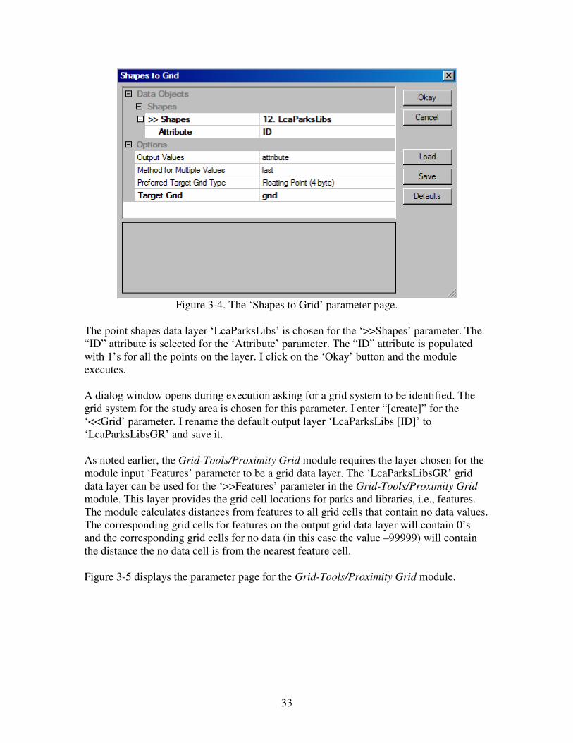
33
Figure 3-4. The ‘Shapes to Grid’ parameter page.
The point shapes data layer ‘LcaParksLibs’ is chosen for the ‘>>Shapes’ parameter. The
“ID” attribute is selected for the ‘Attribute’ parameter. The “ID” attribute is populated
with 1’s for all the points on the layer. I click on the ‘Okay’ button and the module
executes.
A dialog window opens during execution asking for a grid system to be identified. The
grid system for the study area is chosen for this parameter. I enter “[create]” for the
‘<<Grid’ parameter. I rename the default output layer ‘LcaParksLibs [ID]’ to
‘LcaParksLibsGR’ and save it.
As noted earlier, the Grid-Tools/Proximity Grid module requires the layer chosen for the
module input ‘Features’ parameter to be a grid data layer. The ‘LcaParksLibsGR’ grid
data layer can be used for the ‘>>Features’ parameter in the Grid-Tools/Proximity Grid
module. This layer provides the grid cell locations for parks and libraries, i.e., features.
The module calculates distances from features to all grid cells that contain no data values.
The corresponding grid cells for features on the output grid data layer will contain 0’s
and the corresponding grid cells for no data (in this case the value –99999) will contain
the distance the no data cell is from the nearest feature cell.
Figure 3-5 displays the parameter page for the Grid-Tools/Proximity Grid module.

34
Figure 3-5. The Grid-Tools/Proximity Grid module parameter page.
The ‘LcaParksLibsGR’ grid data layer is chosen for the ‘>>Features’ parameter and
“[create]” is selected for the required output ‘<<Distance’ parameter. I click the ‘Okay’
button and the module executes.
The output grid data layer is named ‘Distance’. The Grid-Tools/Proximity Grid module
calculated distance values from parks and library grid cells to all cells containing the no
data value. This includes grid cells outside of the study area but still within the grid
system. Parks and library grid cells from the ‘LcaParksLibsGR’ layer, on the ‘Distance’
layer, contain 0’s and no data cells from the ‘LcaParksLibsGR’ layer contain distance
values representing the distance to the nearest park or library to the cell.
I do not want the data values outside of the study area that contain data values to
contribute to the solution. I use the Grid-Tools/Grid Masking module to convert these
data values to no data -99999 values. Figure 3-6 displays the parameter page for the Grid-
Tools/Grid Masking module.
Figure 3-6. The parameter page for the Grid-Tools/Grid Masking module.

35
The default output layer from the Proximity Grid module, ‘Distance’, is chosen for the
input ‘>>Grid’ parameter and the “[create]” option for the ‘<Masked Grid’ output
parameter is entered. The grid data layer ‘LcaStudyAreaGR’ is chosen for the ‘>>Mask’
input parameter. I click the ‘Okay’ button and the module executes.
The default name for the output layer is ‘Masked Grid’. I rename ‘Masked Grid’ to
‘LcaParksLibsDistGR’ and save it.
The data range for the ‘LcaParksLibsDistGR’ layer is 0 to 46243.03125. On this layer,
values are distances grid cells are from parks and libraries. The intent is to develop a
factor element cost layer that contains data values rescaled into continuous values
between 0 and 1 for the continuous data range from 0 to 46243.03125. Because impacts
are higher the closer a transmission line is to a park or library, the continuous data range
is from 0 to 1 where the lowest impact is 0 (a cell furthest from a park or library) and the
impact increases from 0 to 1 (a cell adjacent to a park or library).
The Grid – Calculus/Grid Normalisation module is used to rescale the data values on the
‘LcaParksLibsDistGR’ layer. Figure 3-7 displays the parameter page for the Grid –
Calculus/Grid Normalisation module.
Figure 3-7. The parameter page for the Grid – Calculus/ Grid Normalisation module.
The ‘LcaParksLibsDistGR’ grid data layer is chosen for the input ‘>>Grid’ parameter
and “[create]” for the output ‘<<Normalised Grid’ parameter. The data range of the input
grid data layer is rescaled to continuous values between 0 and 1. The minimum and
maximum values are entered for the ‘Target Range’ parameter. I click the ‘Okay’ button
and the module executes.
This is one of the factor elements where the existing data range of continuous values is
inversely rescaled to values between 1 and 0. The data value range for the input layer is 0

36
to 46243.03125 and it is rescaled such that rescaled continuous values decrease from 1
for 0 to 0 for 46243.03125. This is because the nearer the grid cell is to a park or library,
the higher the impact cost.
The output grid data layer ‘Normalised Grid’ is renamed ‘LcaParksLibsDistGRNM’ and
saved.
The data values on the ‘LcaParksLibsDistGRNM’ layer range from 0 to 1 and define an
increasing range of impact, 1 being the highest level for cells adjacent to a park or library
and 0 for cells the most distant from a park or library. Cells in between have values
decreasing from 0 to 1.
Visibility From Highly Valued Cultural and Recreational Sites
As noted in the preceding section, highly valued cultural and recreational sites are
defined as county parks, non-county parks and libraries. The ‘LcaParksLibs’ point shapes
data layer contains point objects that represent these sites. There are 40 within the study
area. The Grid-Gridding/Shapes to Grid module was used to create a grid data layer
version of the point shapes data layer. It is named ‘LcaParksLibsGR’.
Delineating a viewshed is a task often associated with assessing the visual impact of a
proposed construction project. The land area that can be seen from a project is defined as
its’ viewshed. The viewshed is frequently divided into three zones: foreground, middle
ground, and background. Foreground extends to ½ mile, middle ground from ½ mile to 3
miles, and background greater than 3 miles. In this tutorial, a viewshed for a site is
defined as the grid cells that can be seen from the site that are within 3 miles of the site.
Three miles is the boundary between the middle ground and the background.
Two common approaches for determining whether a location is visible from our proposed
transmission corridor exist. One way is to use visibility as an evaluation criterion after a
proposed corridor location is identified. A series of “observer” locations would be
defined along the proposed corridor path. A viewshed would be calculated for each
observer. The viewsheds would be aggregated. A determination would then be made as to
how many of the cultural and recreation sites are within the aggregate viewshed.
A second approach, the one used in this tutorial, is to calculate the viewshed for each
recreation/library site, aggregate the viewsheds, and define a “visibility” grid data layer.
Cell values on the layer indicate if a cell is visible from a site, and, if visible, from how
many sites. The more times a cell can be viewed from sites, the higher the impact cost.
Since I am not considering view blocking vegetation and buildings in determining the
viewsheds, this might be considered a worse case scenario. The inclusion of vegetation
and buildings would reduce the number of visible grid cells.
The Terrain Analysis – Lighting, Visibility/Visibility (single point) [interactive] module is
used for calculating the viewshed of a single point. Unfortunately, the Terrain Analysis –
Lighting, Visibility/Visibility (single point) [interactive] module does not have a distance
limiting option for the viewing distance. As you will see below, the Grid Calculus
37
module can be used with the default output ‘Visibility’ layer to limit the viewshed
distance to three miles.
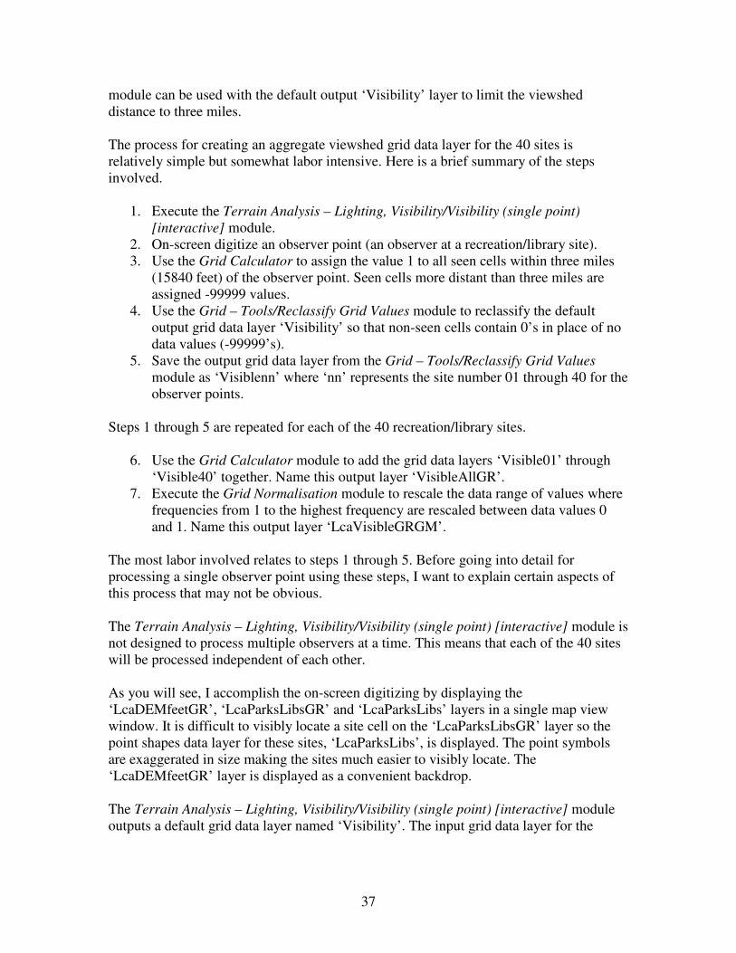
The process for creating an aggregate viewshed grid data layer for the 40 sites is
relatively simple but somewhat labor intensive. Here is a brief summary of the steps
involved.
1. Execute the Terrain Analysis – Lighting, Visibility/Visibility (single point)
[interactive] module.
2. On-screen digitize an observer point (an observer at a recreation/library site).
3. Use the Grid Calculator to assign the value 1 to all seen cells within three miles
(15840 feet) of the observer point. Seen cells more distant than three miles are
assigned -99999 values.
4. Use the Grid – Tools/Reclassify Grid Values module to reclassify the default
output grid data layer ‘Visibility’ so that non-seen cells contain 0’s in place of no
data values (-99999’s).
5. Save the output grid data layer from the Grid – Tools/Reclassify Grid Values
module as ‘Visiblenn’ where ‘nn’ represents the site number 01 through 40 for the
observer points.
Steps 1 through 5 are repeated for each of the 40 recreation/library sites.
6. Use the Grid Calculator module to add the grid data layers ‘Visible01’ through
‘Visible40’ together. Name this output layer ‘VisibleAllGR’.
7. Execute the Grid Normalisation module to rescale the data range of values where
frequencies from 1 to the highest frequency are rescaled between data values 0
and 1. Name this output layer ‘LcaVisibleGRGM’.
The most labor involved relates to steps 1 through 5. Before going into detail for
processing a single observer point using these steps, I want to explain certain aspects of
this process that may not be obvious.
The Terrain Analysis – Lighting, Visibility/Visibility (single point) [interactive] module is
not designed to process multiple observers at a time. This means that each of the 40 sites
will be processed independent of each other.
As you will see, I accomplish the on-screen digitizing by displaying the
‘LcaDEMfeetGR’, ‘LcaParksLibsGR’ and ‘LcaParksLibs’ layers in a single map view
window. It is difficult to visibly locate a site cell on the ‘LcaParksLibsGR’ layer so the
point shapes data layer for these sites, ‘LcaParksLibs’, is displayed. The point symbols
are exaggerated in size making the sites much easier to visibly locate. The
‘LcaDEMfeetGR’ layer is displayed as a convenient backdrop.
The Terrain Analysis – Lighting, Visibility/Visibility (single point) [interactive] module
outputs a default grid data layer named ‘Visibility’. The input grid data layer for the

38
module is the ‘LcaDEMfeetGR’ layer that provides the elevation information for the
analysis.
The ‘Height’ parameter is used to set the height of the observer above the terrain. I am
setting the height of the observer at 5 feet above the terrain. There are several options for
the ‘Unit’ parameter depending on the objective. My purpose is to define a viewshed for
each site identifying visible grid cells within 3 miles of the site. So I choose the
“Distance” option to have distance values calculated for seen grid cells. On the default
grid data layer output, ‘Visibility’, visible cells will contain a distance value and non-
visible cells will contain no data values –99999.
The goal for the viewshed version of the ‘Visibility’ grid data layer is for seen grid cells
within three miles of the observer point to contain 1’s and not seen cells to contain 0’s. If
the not seen cells contain the no data value the layers cannot be added together to create
an aggregate layer. The ‘Visibility’ layer contains distance values for seen cells greater
than three miles from the observer point. In step 3, the Grid – Calculus/Grid Calculator
module is used for converting distance values in seen grid cells to 1’s if the grid cell is
within three miles of the observer point. The formula used for this is:
ifelse(lt(a,15840.00001),1,-99999)
Grid cells either contain a distance value or a no data value of –99999. The variable “a”
represents the input grid data layer. The equation checks to see if the distance value for a
cell is less than 15840.00001 (three miles). If it is less than 15840.00001, the value 1 is
output to the corresponding cell in the output layer. If the value is greater than
15840.00001, the no data value –99999 is output to the corresponding output grid cell.
One of the processing steps is to add the 40 site viewsheds together into a single
aggregate layer. This will be done using the Grid Calculator module to add the layers
together. No data cells in a layer, however, will only generate no data cells regardless of
whether corresponding cells in other layers contain valid data values. This means I must
convert all no data values of –99999 to 0 values. Thus, the fourth step listed above, is to
use the Grid – Tools/Reclassify Grid Values module to change the –99999 no data value
to 0 for each ‘Visible…TEMP’ layer.
The modified ‘Visible’ grid data layer is saved with a name that includes a reference to
the site number the viewshed is based on. The site number is determined by the “SITE”
attribute in the point shapes data layer ‘LcaParksLibs’. As you recall, defining a “SITE”
field was described earlier related to the ‘LcaParksLibs’ point shapes data layer. I
manually entered the numeric data for the “SITE” attribute. Each site was assigned a
unique number, 1 through 40.
This next section describes the processing steps for site 1.
Prior to step 1, I create a map display window displaying the two grid data layers
‘LcaDEMfeetGR’ and ‘LcaParksLibsGR’ and the point shapes data layer ‘LcaParksLibs’.

39
Make sure the order for the layers in the map view window is the ‘LcaDEMfeetGR’ layer
the bottom layer and the ‘LcaParksLibs’ point shapes layer the top. I choose the
“Transparent” option for the ‘Fill Style’ parameter in the ‘Settings’ tab for the
‘LcaParksLibs’ point shapes data layer. In addition, I choose the “SITE” attribute in the
“Labels” section of the settings so the site numbers will be displayed alongside the point
object symbols. This map display window is going to be used for the on-screen digitizing
of the observer points.
1. Execute the Terrain Analysis – Lighting, Visibility/Visibility (single point) [interactive]
module.
Figure 3-8 displays the Terrain Analysis – Lighting, Visibility/Visibility (single point)
[interactive] module parameter page.
Figure 3-8. The ‘Visibility (single point)’ parameter page.
The input grid data layer for the ‘>>Elevation’ parameter is ‘LcaDEMfeetGR’. The
“[create]” option is chosen for the output parameter ‘<<Visibility’. The default name for
the output layer is “Visibility”. The value entered for the ‘Height’ parameter represents
the height of the observer above the terrain. In this tutorial, the observer is 5’ above the
terrain (representing an estimated average eye height for a person). The output units on
the output layer are chosen with the ‘Unit’ parameter. I have chosen “Distance” as I want
the output values to represent the distance a seen cell is from the observer point. I click
the ‘Okay’ button and the module executes.
2. On-screen digitize an observer point (an observer at one of the recreation/library sites).

40
Figure 3-9. Zoomed-in portions of my on-screen digitizing map window.
The image on the left in Figure 3-9 is a zoomed in portion of the lower section of the
image on the right. I can see the label “40” near the bottom on the right in the zoomed out
view. Site 1 is my first site to process and it is quite near site 40. The black grid cells are
the grid cells representing the site locations on the ‘LcaParksLibsGR’ grid data layer. As
you can see, using the zoom tool ( ) on the Tool Bar makes it easier to on-screen
digitize the observer point.
The Action ( ) tool on the Tool Bar is used to on-screen digitize. I choose the Action
tool from the Tool Bar, move the cursor arrow over the black grid cell representing site 1,
and press the left key on the mouse. After I click the button the module creates the
‘Visibility’ layer and proceeds to calculate the viewshed. When the layer is complete, a
map view window displaying it will appear in the work area. What I usually do is click
on the ‘Visibility’ layer name in the ‘Data’ tab area of the Workspace once it appears and
display the layer in my on-screen digitizing map window.
The Terrain Analysis – Lighting, Visibility/Visibility (single point) [interactive] module is
an interactive module. This means I terminate its execution by moving the mouse pointer
to the Menu Bar and clicking on the ‘Modules’ option. At the bottom of the drop-down
list of options, “Visibility/Visibility (single point) [interactive]” is displayed with a check
to its left. The check means the module is running. I click on the name to the right of the
check and this stops the module from running.
3. Use the Grid Calculator to assign the value 1 to all seen cells with distance (from the
observer) values less then 15840 and assign the no data value –99999 to all seen cells
with a distance value greater than 15840.
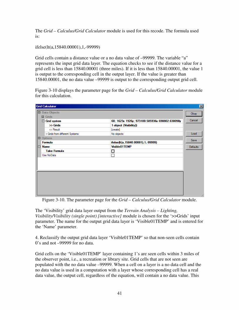
41
The Grid – Calculus/Grid Calculator module is used for this recode. The formula used
is:
ifelse(lt(a,15840.00001),1,-99999)
Grid cells contain a distance value or a no data value of –99999. The variable “a”
represents the input grid data layer. The equation checks to see if the distance value for a
grid cell is less than 15840.00001 (three miles). If it is less than 15840.00001, the value 1
is output to the corresponding cell in the output layer. If the value is greater than
15840.00001, the no data value –99999 is output to the corresponding output grid cell.
Figure 3-10 displays the parameter page for the Grid – Calculus/Grid Calculator module
for this calculation.
Figure 3-10. The parameter page for the Grid – Calculus/Grid Calculator module.
The ‘Visibility’ grid data layer output from the Terrain Analysis – Lighting,
Visibility/Visibility (single point) [interactive] module is chosen for the ‘>>Grids’ input
parameter. The name for the output grid data layer is ‘Visible01TEMP’ and is entered for
the ‘Name’ parameter.
4. Reclassify the output grid data layer ‘Visible01TEMP’ so that non-seen cells contain
0’s and not –99999 for no data.
Grid cells on the ‘Visible01TEMP’ layer containing 1’s are seen cells within 3 miles of
the observer point, i.e., a recreation or library site. Grid cells that are not seen are
populated with the no data value –99999. When a cell on a layer is a no data cell and the
no data value is used in a computation with a layer whose corresponding cell has a real
data value, the output cell, regardless of the equation, will contain a no data value. This

42
can be a valid output depending on the situation. However, in this case, I want the no data
values to be data value 0’s. This way the grid cells can be used in an equation involving
other grid data layers with corresponding cells containing valid frequency data. The Grid
– Tools/Reclassify Grid Values module is used to change the –99999 values to 0’s.
Figure 3-11 displays the parameter page for Grid – Tools/Reclassify Grid Values module
set up for this change.
Figure 3-11. The Grid – Tools/Reclassify Grid Values module parameter page.
The ‘Visibile01TEMP’ grid data layer is chosen for the ‘>>Grid’ input parameter and
“[create]” is chosen for the output parameter ‘<<Reclassified Grid’. The default name for
the output grid layer is ‘Reclassified Grid’. Only one value is to be changed so the
“single” option is chosen for the ‘Method’ parameter. The old value, i.e., the no data
value (-99999), is entered for the ‘old value’ parameter and the new value “0” is entered
for the ‘new value’ parameter. The “=” operator is chosen for the ‘operator’ parameter.
The check box for the ‘no data values’ parameter is not checked. The output grid data
layer will not contain any grid cells with no data values.
5. Save the output grid data layer from the Reclassify Grid Values module as ‘Visiblenn’
where ‘nn’ represents an observer point 01 through 40.
The output grid data layer is saved as ‘Visible01’. As a last step I save it.
Steps 1 through 5 were repeated for each of the recreation and library sites. The output
grid data layer names included the site name, e.g., ‘Visible01’ grid data layer was the
viewshed for site 01. A viewshed layer was created for each site. Each of these
‘Visiblenn’ files was saved.

43
6. Use the Grid Calculator module to add grid data layers ‘Visible01’ through
‘Visible40’ together. Name this output layer ‘VisibleAllGR’.
The formula parameter in the Grid – Calculus/Grid Calculator module supports up to 26
variables or layers in an equation, i.e., one for each lower-case character of the alphabet.
This works fine when you do not have more than 26 input layers. In this instance I have
40 input layers. I used 10 layers at a time, creating four interim layers, and then added the
four layers together to create a final composite layer for the addition of all 40 input
layers. Figure 3-12 displays the first execution of this process.
Figure 3-12. The Grid – Calculus/Grid Calculator module parameter page.
I have chosen the first 10 viewshed grid data layers for input for the ‘>>Grids’ parameter.
The equation entered for the ‘Formula’ parameter is a simple addition for the 10 input
layers “a+b+c…”. This first of four interim outputs is named ‘Visible01-10’.
Following the creation of these four interim output grid data layers, I executed the Grid –
Calculus/Grid Calculator module a fifth time adding the four interim layers together to
create a temporary layer named ‘VisibleAllTEMPGR’. On this temporary layer, the
highest frequency for a visible cell is 12. This means that the cell can be seen by 12 of the
observer points/sites. All other grid cells contain 0’s or values 1 through 11.
There are grid cells on the ‘VisibleAllTEMPGR’ layer outside of the study area that
contain data values. Before applying the Grid Normalisation module, I want to mask out
these grid cells converting any data values to no data values. I use the Grid – Tools/Grid
Masking module for this purpose. Figure 3-13 displays the parameter page for the
module.
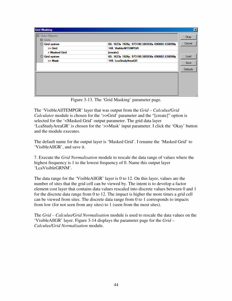
44
Figure 3-13. The ‘Grid Masking’ parameter page.
The ‘VisibleAllTEMPGR’ layer that was output from the Grid – Calculus/Grid
Calculator module is chosen for the ‘>>Grid’ parameter and the “[create]” option is
selected for the ‘<Masked Grid’ output parameter. The grid data layer
‘LcaStudyAreaGR’ is chosen for the ‘>>Mask’ input parameter. I click the ‘Okay’ button
and the module executes.
The default name for the output layer is ‘Masked Grid’. I rename the ‘Masked Grid’ to
‘VisibleAllGR’, and save it.
7. Execute the Grid Normalisation module to rescale the data range of values where the
highest frequency is 1 to the lowest frequency of 0. Name this output layer
‘LcaVisibleGRNM’.
The data range for the ‘VisibleAllGR’ layer is 0 to 12. On this layer, values are the
number of sites that the grid cell can be viewed by. The intent is to develop a factor
element cost layer that contains data values rescaled into discrete values between 0 and 1
for the discrete data range from 0 to 12. The impact is higher the more times a grid cell
can be viewed from sites. The discrete data range from 0 to 1 corresponds to impacts
from low (for not seen from any sites) to 1 (seen from the most sites).
The Grid – Calculus/Grid Normalisation module is used to rescale the data values on the
‘VisibleAllGR’ layer. Figure 3-14 displays the parameter page for the Grid –
Calculus/Grid Normalisation module.

45
Figure 3-14. The Grid – Calculus/Grid Normalisation module parameter page.
The ‘VisibleAllGR’ grid data layer is chosen for the input ‘>>Grid’ parameter and
“[create]” for the output ‘<<Normalised Grid’ parameter. The data range of the input grid
data layer is 0 to 12. This range is rescaled to discrete values between 0 and 1. The
minimum and maximum values are entered for the ‘Target Range’ parameter. I click the
‘Okay’ button and the module executes.
The output grid data layer ‘Normalised Grid’ is renamed ‘LcaVisibleAllGRNM’ and
saved. The data values on the ‘LcaVisibleAllGRNM’ layer range from 0 to 1 and define
an increasing range of impact, 0 for cells not seen by any site and 1 being the highest
level for cells seen by the most sites. Cells in between have values increasing from 0 to 1.
This completes the development of this data element, “Visibility From Highly Valued
Cultural and Recreational Sites”.
The next two data factor elements are quite similar to these first two.
Distance From Sensitive Non-Residential Buildings
Overview
1. Add a new attribute named “SITE” to the sensitive non-residential buildings
shapes data layer, ‘LcaSensBldg’.
2. Convert the ‘LcaSensBldg’ shapes layer to a grid data layer using the Grid-
Gridding/Shapes to Grid module. Name the new grid layer ‘LcaSensBldgGR’.
3. Use the grid layer ‘LcaSensBldgGR’ as input to the Grid-Tools/Proximity Grid
module to produce a layer with grid cells containing distances from features
values.
4. Apply the Grid-Tools/Grid Masking module to recode data values outside of the
study area to no data values (-99999).
5. Rescale the data range of distance values to a continuous data range from 0 to 1
with the Grid – Calculus/Grid Normalisation module.

46
Description
The ‘LcaSensBldg’ point shapes data layer contains 43 point objects representing
“sensitive non-residential buildings” for the study area. Unfortunately, due to small
physical size and low population, there are not many buildings that would fit a definition
of being sensitive. I am using a combination of commercial and industrial buildings as a
hypothetical representation of “sensitive non-residential buildings”.
Before incorporating this factor element into the model, I want to add a new attribute to
the linked attribute table for the ‘LcaSensBldg’ point shapes data layer. The attribute will
be named “SITE”. I will manually enter a unique site number between 1 and 43 in the
“SITE” attribute for each of the 43 point objects. You will recall that I created a similar
attribute for the ‘LcaParksLibs’ point shapes data layer. The “SITE” attribute is used
during the on-screen digitizing process for creating viewsheds for the “Visibility From
Sensitive Non-Residential Buildings” element.
The Grid-Tools/Proximity Grid module is used to calculate distances from sensitive non-
residential buildings grid cells to no data grid cells. The input layer of features for this
module has to be a grid data layer. This means that I need to create a grid version of my
point shapes data layer ‘LcaSensBldg’ that contains point objects for the non-residential
buildings.
I use the Grid-Gridding/Shapes to Grid module to develop a grid version of the point
shapes layer. Figure 3-15 displays the parameter page for this module.
Figure 3-15. The parameter page for the Grid-Gridding/Shapes to Grid module.
The point shapes data layer ‘LcaSensBldg’ is chosen for the ‘>>Shapes’ parameter. The
“ID” attribute is selected for the ‘Attribute’ parameter. The “ID” attribute is populated
with 2’s for all the points on the layer. The “grid” option is chosen for the ‘Target Grid’
parameter. I click the ‘Okay’ button and the module executes.
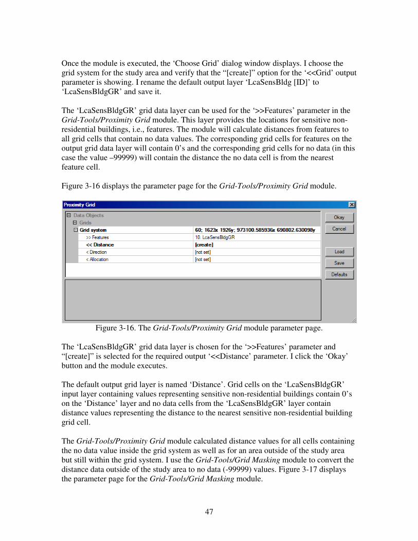
47
Once the module is executed, the ‘Choose Grid’ dialog window displays. I choose the
grid system for the study area and verify that the “[create]” option for the ‘<<Grid’ output
parameter is showing. I rename the default output layer ‘LcaSensBldg [ID]’ to
‘LcaSensBldgGR’ and save it.
The ‘LcaSensBldgGR’ grid data layer can be used for the ‘>>Features’ parameter in the
Grid-Tools/Proximity Grid module. This layer provides the locations for sensitive non-
residential buildings, i.e., features. The module will calculate distances from features to
all grid cells that contain no data values. The corresponding grid cells for features on the
output grid data layer will contain 0’s and the corresponding grid cells for no data (in this
case the value –99999) will contain the distance the no data cell is from the nearest
feature cell.
Figure 3-16 displays the parameter page for the Grid-Tools/Proximity Grid module.
Figure 3-16. The Grid-Tools/Proximity Grid module parameter page.
The ‘LcaSensBldgGR’ grid data layer is chosen for the ‘>>Features’ parameter and
“[create]” is selected for the required output ‘<<Distance’ parameter. I click the ‘Okay’
button and the module executes.
The default output grid layer is named ‘Distance’. Grid cells on the ‘LcaSensBldgGR’
input layer containing values representing sensitive non-residential buildings contain 0’s
on the ‘Distance’ layer and no data cells from the ‘LcaSensBldgGR’ layer contain
distance values representing the distance to the nearest sensitive non-residential building
grid cell.
The Grid-Tools/Proximity Grid module calculated distance values for all cells containing
the no data value inside the grid system as well as for an area outside of the study area
but still within the grid system. I use the Grid-Tools/Grid Masking module to convert the
distance data outside of the study area to no data (-99999) values. Figure 3-17 displays
the parameter page for the Grid-Tools/Grid Masking module.

48
Figure 3-17. The Grid-Tools/Grid Masking module parameter page.
The default output layer from the Proximity Grid module, ‘Distance’, is chosen for the
input ‘>>Grid’ parameter and the “[create]” option for the ‘<Masked Grid’ output
parameter is entered. The grid data layer ‘LcaStudyAreaGR’ is chosen for the ‘>>Mask’
input parameter. I click the ‘Okay’ button and the module executes.
The default name for the output layer is ‘Masked Grid’. I rename the ‘Masked Grid’ to
‘LcaSensBldgDistGR’ layer and save it.
The data range for the ‘LcaSensBldgDistGR’ layer is 0 to 54269.890625. On this layer,
data values are distances grid cells are to sensitive buildings. The intent is to develop a
factor element cost layer that contains data values rescaled into continuous values
between 0 and 1 for the continuous data range from 0 to 54269.890625. Because impacts
are higher the closer a transmission line is to a sensitive building, the continuous data
range from 0 to 1 where the lowest impact is 0 (a cell furthest from a sensitive building)
and the impact increases from 0 to 1 (a cell adjacent to a sensitive building).
The Grid – Calculus/Grid Normalisation module is used to rescale the data values on the
‘LcaSensBldgDistGR’ layer. Figure 3-18 displays the parameter page for the Grid –
Calculus/Grid Normalisation module.

49
Figure 3-18. The parameter page for the Grid – Calculus/Grid Normalisation module.
The ‘LcaSensBldgDistGR’ grid data layer is chosen for the input ‘>>Grid’ parameter and
“[create]” for the output ‘<<Normalised Grid’ parameter. The data range of the input grid
data layer is rescaled to continuous values between 0 and 1. The minimum and maximum
values are entered for the ‘Target Range’ parameter. I click the ‘Okay’ button and the
module executes.
This is one of the factor elements where the existing data range of continuous values is
inversely rescaled to values between 0 and 1. The data value range for the input layer is 0
to 54269.890625 and it is rescaled such that rescaled continuous values decrease from 1
for 0 to 0 for 54269.890625. This is because the nearer the grid cell is to a sensitive
building, the higher the impact cost.
The output grid data layer ‘Normalised Grid’ is renamed ‘LcaSensBldgDistGRNM’ and
saved.
Visibility From Sensitive Non-Residential Buildings
The procedures for handling “Visibility From Sensitive Non-Residential Buildings” are
quite similar to the ones for “Visibility From Highly Valued Cultural and Recreational
Sites”.
The ‘LcaSensBldg’ shapes data layer contains 43 point objects representing “sensitive”
non-residential buildings. The Grid-Gridding/Shapes to Grid module was used to create a
grid data layer version of the point shapes data layer. It is named ‘LcaSensBldgGR’.
The viewshed for a “sensitive” non-residential building is defined the same way as one
for a cultural or recreation site. The viewshed is made up of grid cells that can be seen
from the observer point that are within three miles of the of the observer point/site. As
noted earlier, three miles is the boundary between middle ground and background zones.

50
The viewsheds for each of the sites will be calculated. The 43 viewsheds together define
a “visibility” grid data layer for the 43 buildings. A cell value of 0 on this layer means the
cell is not seen from any of the 43 sites. A value greater than 1 indicates that the cell is
seen and from how many sites it is seen. Since I am not considering view blocking
vegetation and buildings in determining the viewsheds, this approach might be
considered a worse case scenario. The inclusion of vegetation and buildings would
reduce the number of visible grid cells.
The Terrain Analysis – Lighting, Visibility/Visibility (single point) [interactive] module is
used for calculating the viewshed of a single point. As pointed out earlier, this module
does not have an option for restricting the viewing distance. Restricting the viewing
distance to three miles is handled with the Grid – Calculator/Grid Calculus module and
described below.
The process for creating an aggregate viewshed grid data layer is relatively simple but
somewhat labor intensive. The summary of this process provided earlier is recalled
below.
1. Execute the Terrain Analysis – Lighting, Visibility/Visibility (single point)
[interactive] module.
2. On-screen digitize an observer point (an observer at one of the sensitive
buildings).
3. Use the Grid Calculator to assign the value 1 to all seen cells within three miles
(15840 feet) of the observer point. Seen cells more distant than three miles are
assigned -99999 values.
4. Reclassify the default output grid data layer ‘Visibility’ with the Grid –
Tools/Reclassify Grid Values module so that non-seen cells contain 0’s in place of
no data values (-99999’s).
5. Save the output grid data layer from the Grid – Tools/Reclassify Grid Values
module as ‘Visibldgnn’ where ‘nn’ represents the site number 01 through 43 for
the observer points.
These steps, 1 through 5, are repeated for each of the 43 sensitive buildings.
6. Use the Grid Calculator module to add the grid data layers ‘Visibldg01’ through
‘Visibldg43’ together. Name this output layer ‘VisibldgAllGR’.
7. Execute the Grid Normalisation module to rescale the data range of values where
frequencies from 1 to the highest frequency are rescaled between data values 0
and 1. Name this output layer ‘LcaVisibldgGRNM’.
The Terrain Analysis – Lighting, Visibility/Visibility (single point) [interactive] module is
executed for a single observer point at a time. This module is not designed to process
multiple observers. This means that each of the 43 sites will be processed independent of
each other.

51
As you will see, I accomplish the on-screen digitizing by displaying the
‘LcaDEMfeetGR’, ‘LcaSensBldgGR’ and ‘LcaSensBldg’ layers in a single map view
window. It is difficult to visibly locate a site cell on the ‘LcaSensBldgGR’ layer so the
point shapes data layer for these sites, ‘LcaSensBldg’, is displayed. The point symbols
are exaggerated in size making the sites much easier to visibly locate. The
‘LcaDEMfeetGR’ layer is displayed as a convenient backdrop.
The Terrain Analysis – Lighting, Visibility/Visibility (single point) [interactive] module
outputs a default grid data layer named ‘Visibility’. The input grid data layer for the
module is the ‘LcaDEMfeetGR’ layer that provides the elevation information for the
analysis.
The ‘Height’ parameter is used to set the height of the observer above the terrain. I am
setting the height of the observer at 5 feet above the terrain. There are several options for
the ‘Unit’ parameter depending on your purpose. The purpose is to define a viewshed for
each site identifying visible grid cells within 3 miles of the site. So I choose the
“Distance” option for this parameter. This means that the data values stored in seen grid
cells is the distance the grid cell is from the observer point. On the default grid data layer
output, ‘Visibility’, visible cells will contain a distance value and non-visible cells will
contain no data values –99999.
The goal for the viewshed version of the ‘Visibility’ grid data layer is for seen grid cells
within three miles of the observer point to contain 1’s and not seen cells to contain 0’s.
The ‘Visibility’ layer, however, contains distance values for seen cells greater than three
miles from the observer point. In step 3, the Grid – Calculus/Grid Calculator module is
used to convert distance values in seen grid cells to 1’s if the grid cell is within three
miles of the observer point. The formula used for this is:
ifelse(lt(a,15840.00001),1,-99999)
Grid cells either contain a distance value or a no data value of –99999. The variable “a”
represents the input grid data layer. The equation checks to see if the distance value for a
cell is less than 15840.00001 (three miles). If it is less than 15840.00001, the value 1 is
output to the corresponding cell in the output layer. If the value is greater than
15840.00001, the no data value –99999 is output to the corresponding output grid cell.
One of the processing steps is to add all the 43 site viewsheds together into a single
aggregate layer. This will be done using the Grid Calculator to add the layers together.
No data cells in a layer, however, will only generate no data cells regardless of whether
corresponding cells in other layers contain valid data values. This means I must convert
all no data values of –99999 to 0 values. Thus, the fourth step listed above, is to use the
Grid – Tools/Reclassify Grid Values module to change the –99999 no data value to 0 for
each ‘Visibldg…TEMP’ layer.
The modified ‘Visibility’ grid data layer is saved with a name that includes a reference to
the site number the viewshed is based on. The site number is determined by the “SITE”

52
attribute in the point shapes data layer ‘LcaSensBldg’. Defining a “SITE” field for the
‘LcaSensBldg’ point shapes data layer was described earlier. I manually entered the
numeric data for the “SITE” attribute. Each site was assigned a unique number, 1 through
43.
This next section describes the processing steps for site 1. These steps were repeated for
sites 02 through 43.
Prior to step 1, I create a map display window displaying the two grid data layers
‘LcaDEMfeetGR’ and ‘LcaSensBldgGR’ and the point shapes data layer ‘LcaSensBldg’.
Make sure the order for the layers in the map view window is the ‘LcaDEMfeetGR’ layer
the bottom layer and the ‘LcaSenBldg’ point shapes layer the top. I choose the
“Transparent” option for the ‘Fill Style’ parameter in the ‘Settings’ tab for the
‘LcaSensBldg’ point shapes data layer. In addition, I choose the “SITE” attribute in the
“Labels” section of the settings so the site number will be displayed alongside the point
object symbols. This map display window is going to be used for the on-screen digitizing
of the observer points.
1. Execute the Terrain Analysis – Lighting, Visibility/Visibility (single point) [interactive]
module.
Figure 3-19 displays the Terrain Analysis – Lighting, Visibility/Visibility (single point)
[interactive] module parameter page.
Figure 3-19. The Terrain Analysis – Lighting, Visibility/Visibility (single point)
[interactive] module parameter page.
The input grid data layer for the ‘>>Elevation’ parameter is ‘LcaDEMfeetGR’. The
“[create]” option is chosen for the output parameter ‘<<Visibility’. The default name for
the output layer is “Visibility”. The value entered for the ‘Height’ parameter represents
the height of the observer above the terrain. In this example, the observer is 5’ above the
terrain (representing an estimated average eye height for a person, for example). The
output units on the output layer are chosen with the ‘Unit’ parameter. I have chosen

53
“Distance” as I want the output values to represent the distance a seen cell is from the
observer point. I click on the ‘Okay’ button and the module executes.
2. On-screen digitize an observer point (an observer at one of the sensitive building sites).
Figure 3-20. Zoomed-in portions of my on-screen digitizing map window.
The image on the left in Figure 3-20 is a zoomed in portion of the upper right section of
the image on the right. You can see site number 42 above sites 10 and 34 in the image on
the right. Site 1 is going to be my first site to process. It is located in the clump of points
that includes points 27 and 28. The black grid cells appearing within the circles are the
grid cells representing the sites on the ‘LcaSensBldgGR’ grid data layer. As you can see,
using the zoom tool ( ) on the Tool Bar makes it easier to on-screen digitize the
observer point.
The Action ( ) tool on the Tool Bar is used to on-screen digitize. I choose the Action
tool from the Tool Bar, move the cursor arrow over the black grid cell for site 1, and
press the left key on the mouse. After I click the button the module creates the ‘Visibility’
layer and proceeds to create the viewshed. When the layer is complete, a map window
displaying it will appear in the work area. What I usually do is click on the ‘Visibility’
layer name in the ‘Data’ tab area of the Workspace once it appears and display the layer
in my on-screen digitizing map window.
The Terrain Analysis – Lighting, Visibility/Visibility (single point) [interactive] module is
an interactive module. This means I terminate its execution by moving the mouse pointer
to the Menu Bar and clicking on the ‘Modules’ option. At the bottom of the drop-down
list of options, “Visibility/Visibility (single point) [interactive]” is displayed with a check
to its left. The check means the module is running. I click on the name to the right of the
check and this stops the module from running.
3. Use the Grid Calculator to assign the value 1 to all seen cells with distance (from the
observer) values less then 15840 and assign the value -99999 to all seen cells with a
distance value greater than 15840.

54
The Grid – Calculus/Grid Calculator module is used to make this recode. The formula
used is:
ifelse(lt(a,15840.00001),1,-99999)
Grid cells contain a distance value or a no data value of –99999. The variable “a”
represents the input grid data layer. The equation checks to see if the distance value for a
grid cell is less than 15840.00001 (three miles). If it is less than 15840.00001, the value 1
is output to the corresponding cell in the output layer. If the value is greater than
15840.00001, the no data value –99999 is output to the corresponding output grid cell.
Figure 3-21 displays the parameter page for the Grid – Calculus/Grid Calculator module
for this calculation.
Figure 3-21. The parameter page for the Grid – Calculus/Grid Calculator module.
The ‘Visibility’ grid data layer output from the Terrain Analysis – Lighting,
Visibility/Visibility (single point) [interactive] module is chosen for the ‘>>Grids’ input
parameter. The name for the output grid data layer is ‘Visibldg01TEMP’ and is entered
for the ‘Name’ parameter.
4. Reclassify the default output grid data layer ‘Visibldg01TEMP’ so that non-seen cells
contain 0’s and not –99999 for no data.
The data values on the ‘Visibldg01TEMP’ layer containing 1’s are seen cells within 3
miles of the observer point, i.e., a sensitive non-residential building. Grid cells that are
not seen are populated with the no data value –99999. When a cell on a layer is a no data
cell and the no data value is used in a computation with a layer whose corresponding cell
has a real data value, the output cell, regardless of the equation, will contain a no data
value. This can be a valid output depending on the situation. However, in this case, I

55
really want to replace the no data values with real data values of 0’s. This way the grid
cells can be used in an equation involving other grid data layers with corresponding cells
containing valid frequency data. The Grid – Tools/Reclassify Grid Values module is used
to change the –99999 no data values to real data values of 0’s.
Figure 3-22 displays the parameter page for the Grid – Tools/Reclassify Grid Values
module set up for this change.
Figure 3-22. The Grid – Tools/Reclassify Grid Values module parameter page.
The ‘Visibldg01TEMP’ grid data layer is chosen for the ‘>>Grid’ input parameter and
“[create]” is chosen for the output parameter ‘<<Reclassified Grid’. The default name for
the output grid layer is “Reclassified Grid”. Only one value is to be changed so the
“single” option is chosen for the ‘Method’ parameter. The old value, i.e., the no data
value (-99999), is entered for the ‘old value’ parameter and the new value “0” is entered
for the ‘new value’ parameter. The “=” operator is chosen for the ‘operator’ parameter.
The check box for the ‘no data values’ parameter is not checked. The output grid data
layer will not contain any grid cells with no data values.
5. Save the output grid data layer from the Grid Calculator module as ‘Visibldgnn’
where ‘nn’ represents an observer point 01 through 43.
The output grid data layer is ‘Visibldg01’. As a last step I save it.
Steps 1 through 5 were repeated for each of the sensitive building sites. The output grid
data layer names included the site name, e.g., Visibldg01 grid data layer was the
viewshed for site 1. A viewshed layer was created for each site. Each of these
‘Visibldgnn’ files was saved.
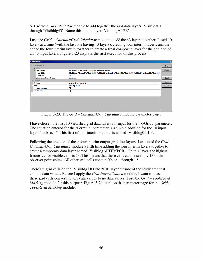
56
6. Use the Grid Calculator module to add together the grid data layers ‘Visibldg01’
through ‘Visibldg43’. Name this output layer ‘VisibldgAllGR’.
I use the Grid – Calculus/Grid Calculator module to add the 43 layers together. I used 10
layers at a time (with the last one having 13 layers), creating four interim layers, and then
added the four interim layers together to create a final composite layer for the addition of
all 43 input layers. Figure 3-23 displays the first execution of this process.
Figure 3-23. The Grid – Calculus/Grid Calculator module parameter page.
I have chosen the first 10 viewshed grid data layers for input for the ‘>>Grids’ parameter.
The equation entered for the ‘Formula’ parameter is a simple addition for the 10 input
layers “a+b+c…”. This first of four interim outputs is named ‘Visibldg01-10’.
Following the creation of these four interim output grid data layers, I executed the Grid –
Calculus/Grid Calculator module a fifth time adding the four interim layers together to
create a temporary data layer named ‘VisibldgAllTEMPGR’. On this layer, the highest
frequency for visible cells is 13. This means that these cells can be seen by 13 of the
observer points/sites. All other grid cells contain 0’s or 1 through 12.
There are grid cells on the ‘VisibldgAllTEMPGR’ layer outside of the study area that
contain data values. Before I apply the Grid Normalisation module, I want to mask out
these grid cells converting any data values to no data values. I use the Grid – Tools/Grid
Masking module for this purpose. Figure 3-24 displays the parameter page for the Grid –
Tools/Grid Masking module.
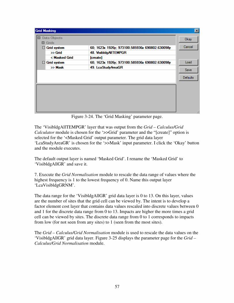
57
Figure 3-24. The ‘Grid Masking’ parameter page.
The ‘VisibldgAllTEMPGR’ layer that was output from the Grid – Calculus/Grid
Calculator module is chosen for the ‘>>Grid’ parameter and the “[create]” option is
selected for the ‘<Masked Grid’ output parameter. The grid data layer
‘LcaStudyAreaGR’ is chosen for the ‘>>Mask’ input parameter. I click the ‘Okay’ button
and the module executes.
The default output layer is named ‘Masked Grid’. I rename the ‘Masked Grid’ to
‘VisibldgAllGR’ and save it.
7. Execute the Grid Normalisation module to rescale the data range of values where the
highest frequency is 1 to the lowest frequency of 0. Name this output layer
‘LcaVisibldgGRNM’.
The data range for the ‘VisibldgAllGR’ grid data layer is 0 to 13. On this layer, values
are the number of sites that the grid cell can be viewed by. The intent is to develop a
factor element cost layer that contains data values rescaled into discrete values between 0
and 1 for the discrete data range from 0 to 13. Impacts are higher the more times a grid
cell can be viewed by sites. The discrete data range from 0 to 1 corresponds to impacts
from low (for not seen from any sites) to 1 (seen from the most sites).
The Grid – Calculus/Grid Normalisation module is used to rescale the data values on the
‘VisibldgAllGR’ grid data layer. Figure 3-25 displays the parameter page for the Grid –
Calculus/Grid Normalisation module.
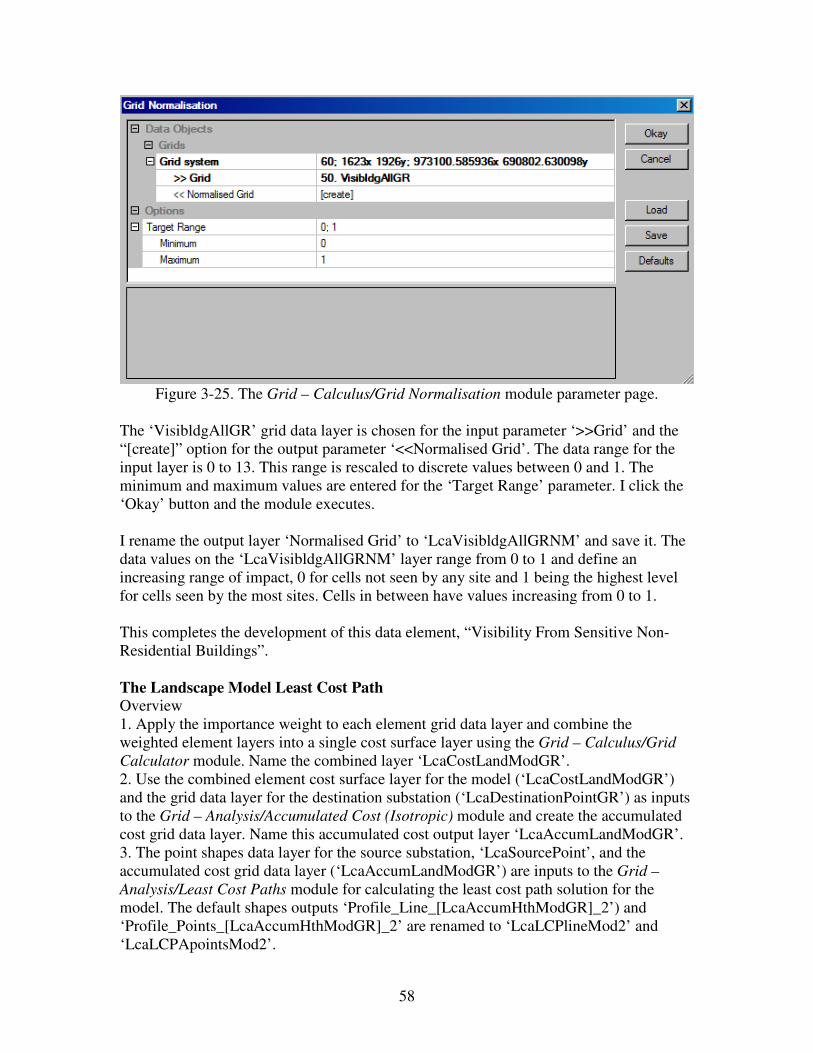
58
Figure 3-25. The Grid – Calculus/Grid Normalisation module parameter page.
The ‘VisibldgAllGR’ grid data layer is chosen for the input parameter ‘>>Grid’ and the
“[create]” option for the output parameter ‘<<Normalised Grid’. The data range for the
input layer is 0 to 13. This range is rescaled to discrete values between 0 and 1. The
minimum and maximum values are entered for the ‘Target Range’ parameter. I click the
‘Okay’ button and the module executes.
I rename the output layer ‘Normalised Grid’ to ‘LcaVisibldgAllGRNM’ and save it. The
data values on the ‘LcaVisibldgAllGRNM’ layer range from 0 to 1 and define an
increasing range of impact, 0 for cells not seen by any site and 1 being the highest level
for cells seen by the most sites. Cells in between have values increasing from 0 to 1.
This completes the development of this data element, “Visibility From Sensitive Non-
Residential Buildings”.
The Landscape Model Least Cost Path
Overview
1. Apply the importance weight to each element grid data layer and combine the
weighted element layers into a single cost surface layer using the Grid – Calculus/Grid
Calculator module. Name the combined layer ‘LcaCostLandModGR’.
2. Use the combined element cost surface layer for the model (‘LcaCostLandModGR’)
and the grid data layer for the destination substation (‘LcaDestinationPointGR’) as inputs
to the Grid – Analysis/Accumulated Cost (Isotropic) module and create the accumulated
cost grid data layer. Name this accumulated cost output layer ‘LcaAccumLandModGR’.
3. The point shapes data layer for the source substation, ‘LcaSourcePoint’, and the
accumulated cost grid data layer (‘LcaAccumLandModGR’) are inputs to the Grid –
Analysis/Least Cost Paths module for calculating the least cost path solution for the
model. The default shapes outputs ‘Profile_Line_[LcaAccumHthModGR]_2’) and
‘Profile_Points_[LcaAccumHthModGR]_2’ are renamed to ‘LcaLCPlineMod2’ and
‘LcaLCPApointsMod2’.

59
Description
The four factor elements of the determinant model have been prepared and are ready to
be combined using the factor element importance weights and the Grid-Calculus/Grid
Calculator module. The model elements and their weights are displayed below.
Distance from highly valued cultural and recreational sites (.10)
Visibility from cultural and recreational sites (.45)
Distance from sensitive non-residential buildings (.10)
Visibility from sensitive non-residential buildings (.35)
These weights are impact weights and they sum to 1.0. The two visibility related
elements account for 80% of the total impact for the model with weights of .45 and .35.
The two distance-related elements each have impact weights of .10.
The Grid-Calculus/Grid Calculator module is going to be used to apply the weights to
the layers and add the layers together in a single execution of the module. Figure 3-26
displays the parameter page for the Grid-Calculus/Grid Calculator module.
Figure 3-26. The parameter page for the Grid-Calculus/Grid Calculator module.
The four factor element grid data layers are entered for the input parameter ‘>>Grids’
value field. The layers are ‘LcaParksLibsDistGRNM’, ‘LcaVisibleAllGRNM’,
‘LcaSensBldgDistGRNM’, and ‘LcaVisibldgAllGRNM’.
The equation entered for the ‘Formula’ parameter is “(a*.10)+(b*.45)+(c*.10)+(d*.35)”.
The lower case characters a, b, c, and d in the equation represent the four grid data layers
in the input parameter value field in the order they appear. The values .10, .45, .10 and
.35 are the pre-defined importance weights. The importance weight for the layer will be
multiplied times the data values in the layer grid cells. The resultants for corresponding
grid cells on the four layers are added together and output to the corresponding grid cell
of the output grid data layer named ‘LcaCostLandModGR’. This is the cost surface layer
for the model.
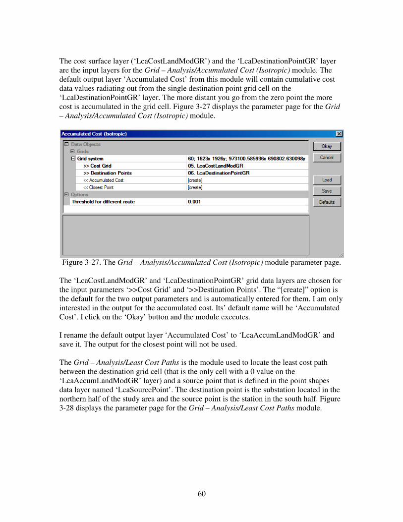
60
The cost surface layer (‘LcaCostLandModGR’) and the ‘LcaDestinationPointGR’ layer
are the input layers for the Grid – Analysis/Accumulated Cost (Isotropic) module. The
default output layer ‘Accumulated Cost’ from this module will contain cumulative cost
data values radiating out from the single destination point grid cell on the
‘LcaDestinationPointGR’ layer. The more distant you go from the zero point the more
cost is accumulated in the grid cell. Figure 3-27 displays the parameter page for the Grid
– Analysis/Accumulated Cost (Isotropic) module.
Figure 3-27. The Grid – Analysis/Accumulated Cost (Isotropic) module parameter page.
The ‘LcaCostLandModGR’ and ‘LcaDestinationPointGR’ grid data layers are chosen for
the input parameters ‘>>Cost Grid’ and ‘>>Destination Points’. The “[create]” option is
the default for the two output parameters and is automatically entered for them. I am only
interested in the output for the accumulated cost. Its’ default name will be ‘Accumulated
Cost’. I click on the ‘Okay’ button and the module executes.
I rename the default output layer ‘Accumulated Cost’ to ‘LcaAccumLandModGR’ and
save it. The output for the closest point will not be used.
The Grid – Analysis/Least Cost Paths is the module used to locate the least cost path
between the destination grid cell (that is the only cell with a 0 value on the
‘LcaAccumLandModGR’ layer) and a source point that is defined in the point shapes
data layer named ‘LcaSourcePoint’. The destination point is the substation located in the
northern half of the study area and the source point is the station in the south half. Figure
3-28 displays the parameter page for the Grid – Analysis/Least Cost Paths module.

61
Figure 3-28. The parameter page for the Grid – Analysis/Least Cost Paths module.
The grid data layer ‘LcaAccumLandModGR’ is chosen for the input ‘>>Accumulated
cost’ parameter. The ‘LcaAccumLandModGR’ layer is the output layer from the Grid –
Analysis/Accumulated Cost (Isotropic) module. The point shapes data layer
‘LcaSourcePoint’ is chosen for the ‘>>Source Point(s)’ input parameter. This layer
contains the point object for the substation located in the southwest quadrant of the study
area. I click on the ‘Okay’ button and the module executes.
This module produces two output shapes layers; one is a point shapes data layer (default
name ‘Profile_Line_[LcaAccumLandModGR]_1’) and the other is a line shapes data
layer (default name ‘Profile_Points_[LcaAccumLandModGR]_1’). The point shapes data
layer has point objects defining the location of the least cost path between the two points.
The line shapes data layer has a line defining the location of the least cost path between
the two points. I rename the default output layers to ‘LcaLCPAlineMod2’ and
‘LcaLCPpointsMod2’ and save both of them.
The maroon line connecting the two substations in Figure 3-29 is the least cost path
solution for this model.
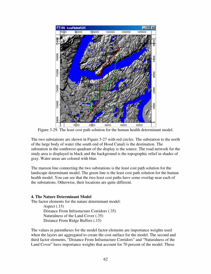
62
Figure 3-29. The least cost path solution for the human health determinant model.
The two substations are shown in Figure 3-27 with red circles. The substation to the north
of the large body of water (the south end of Hood Canal) is the destination. The
substation in the southwest quadrant of the display is the source. The road network for the
study area is displayed in black and the background is the topographic relief in shades of
gray. Water areas are colored with blue.
The maroon line connecting the two substations is the least cost path solution for the
landscape determinant model. The green line is the least cost path solution for the human
health model. You can see that the two least cost paths have some overlap near each of
the substations. Otherwise, their locations are quite different.
4. The Nature Determinant Model
The factor elements for the nature determinant model:
Aspect (.15)
Distance From Infrastucture Corridors (.35)
Naturalness of the Land Cover (.35)
Distance From Ridge Buffers (.15)
The values in parentheses for the model factor elements are importance weights used
when the layers are aggregated to create the cost surface for the model. The second and
third factor elements, “Distance From Infrastucture Corridors” and “Naturalness of the
Land Cover” have importance weights that account for 70 percent of the model. These
63
two elements will have a significant influence on the data values for the cost surface
layer. The remaining two factor elements account for 30 percent of the model.
Generally, this model addresses wildlife habitat concerns. South aspect slopes encourage
upward air currents and can experience use from a high density of important bird species.
Transmission line facilities present on south oriented slopes can have a negative impact
on bird populations. New infrastructure corridors tend to break up wildlife habitat areas.
Transmission lines close to existing infrastructure corridors will have a lower impact on
wildlife habitat areas. Impact on natural vegetation cover is high for the same reasons.
The less natural is the vegetation cover, the lower the impact from a transmission line.
The closer a transmission line is to a buffer area around ridges the higher the potential for
collisions with birds.
Aspect
Overview
Preparation of the ‘LcaAspectDegGR’ grid data layer for aspect data is not too
complicated. The Grid – Calculus/Fuzzify module is used to rescale south facing slopes
to continuous cost data values between 0 and 1. The default output layer from the module
is ‘LcaAspectDegGR [Fuzzified]’ and I rename it ‘LcaAspectDegGRFUZ’.
Description
South aspect slopes are considered to be critical areas because they encourage upward air
currents and can support a high density of important bird species. South-oriented slopes
will experience a higher impact from a transmission corridor compared to other slope
orientations. Aspects plus or minus 10º of due south (180º) will have a high impact value
of 1. Aspects decreasing from 170º to due west (90º) and increasing from 190º to due east
(270º), will have impact values decreasing from 1 to 0.
The ‘LcaAspectDegGR’ grid data layer contains aspect values for the study area. The
Grid – Calculus/Fuzzify module is used to rescale aspect data values to the low to high
impact continuous data value range of 0 to 1.
The Grid – Calculus/Fuzzify module rescales slope aspects between 90º and 170º from 0
increasing to 1, 170º to 190º to 1, and aspects from 190º to 270º decreasing from 1 to 0.
Figure 4-1 displays the parameter page for the Grid – Calculus/Fuzzify module.

64
Figure 4-1. The Grid – Calculus/Fuzzify module parameter page.
The ‘LcaAspectDegGR’ grid data layer containing aspect values in degrees (0 to 360) is
chosen for the input parameter ‘>>Grid’. The “[create]” option is chosen for the output
parameter ‘<<Fuzzified Grid’. The aspect values entered for the control points are 90º,
170º, 190º, and 270º.
Aspect values less than the value for control point ‘A’ are recoded to 0’s. Aspect values
between control points ‘A’ (90º) and ‘B’ (170º) are rescaled to the range 0 increasing to 1
with 170º equal to 1. Data values between control points ‘B’ and ‘C’, i.e., between 170º
and 190º are set to 1. Aspect values between control points ‘C’ (190º) and ‘D’ (270º) are
rescaled decreasing from 1 to 0. Values greater than control point ‘D’, 270º, are set to 0.
I choose the “sigmoidal” option for the ‘Membership Function Type’ as I want the data
values through the control points to have a gradual change rather than a sudden change as
with the “linear” option.
The default output from the module is named ‘LcaAspectDegGR [Fuzzified]’. I rename
the file ‘LcaAspectDegGRFUZ’ and save it.
Distance From Infrastructure Corridors
Overview
1. Use the Shapes – Tools/Shapes Buffer module to develop a polygon shapes data
layer representing road corridors. The ‘LcaStreetCenterlines’ line shapes data
layer is input and the attribute “CORWIDTH” provides corridor widths. The
default output layer is named ‘LcaStreetCenterlines [Buffer]’. I rename it
‘LcaStreetCentBuff’.
2. Convert the polygon shapes layer for road corridors to a grid data layer using the
Grid - Gridding/Shapes to Grid module. Name the new grid layer
‘LcaStreetCentBuffGR’.
65
3. Use the grid data layer ‘LcaStreetCentBuffGR’ as input to the Grid-
Tools/Proximity Grid module to produce a layer with cells containing distance
values to no data cells from features. The default output grid data layer is
‘Distance’.
4. Apply the Grid-Tools/Grid Masking module to recode data values outside of the
study area on the ‘Distance’ data layer to no data values (-99999). The default
output layer from this module is named ‘Masked Grid’. I rename this layer
‘LcaStreetCentBuffDistGR’.
5. Rescale the data range of distance values on the ‘LcaStreetCentBuffDistGR’ layer
to a 0 to 1 range using the Grid – Calculus/Grid Normalisation module. The
default output from this module is named ‘Normalised Grid’. Rename this layer to
‘LcaStrtBuffDistGRNM’.
Description
Building a transmission line close to existing transportation corridors minimizes the
fragmentation of wildlife habitat that results from development of new corridors and new
access. Grid cells further away from existing road corridors will have higher cost values
approaching 1 while cells adjacent and near corridors will have values approaching 0.
The ‘LcaStreetCenterlines’ line shapes data layer contains centerline locations for
highways, roads, streets, etc., in the study area. One of the attributes in the attribute table
linked to the layer is “CORWIDTH”. The values entered for this attribute identify the
corridor width for several road types. There are seven categories of roads and four of
them have corridor widths. Here is the list. The number to the right is the corridor width.
Federal 1500’
State 900’
County 600’
Forest Service 300’
Private 0
GDR 0
City 0
I am going to use the Shapes – Tools/Shapes Buffer module to create a polygon shapes
data layer of road corridors for the four street categories supporting a corridor width.
Figure 4-2 displays the parameter page for the Shapes – Tools/Shapes Buffer module
parameter page.
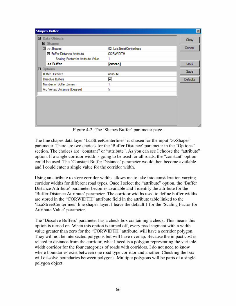
66
Figure 4-2. The ‘Shapes Buffer’ parameter page.
The line shapes data layer ‘LcaStreetCenterlines’ is chosen for the input ‘>>Shapes’
parameter. There are two choices for the ‘Buffer Distance’ parameter in the “Options”
section. The choices are “constant” or “attribute”. As you can see I choose the “attribute”
option. If a single corridor width is going to be used for all roads, the “constant” option
could be used. The ‘Constant Buffer Distance’ parameter would then become available
and I could enter a single value for the corridor width.
Using an attribute to store corridor widths allows me to take into consideration varying
corridor widths for different road types. Once I select the “attribute” option, the ‘Buffer
Distance Attribute’ parameter becomes available and I identify the attribute for the
‘Buffer Distance Attribute’ parameter. The corridor widths used to define buffer widths
are stored in the “CORWIDTH” attribute field in the attribute table linked to the
‘LcaStreetCenterlines’ line shapes layer. I leave the default 1 for the ‘Scaling Factor for
Attribute Value’ parameter.
The ‘Dissolve Buffers’ parameter has a check box containing a check. This means this
option is turned on. When this option is turned off, every road segment with a width
value greater than zero for the “CORWIDTH” attribute, will have a corridor polygon.
They will not be intersected polygons but will have overlap. Because the impact cost is
related to distance from the corridor, what I need is a polygon representing the variable
width corridor for the four categories of roads with corridors. I do not need to know
where boundaries exist between one road type corridor and another. Checking the box
will dissolve boundaries between polygons. Multiple polygons will be parts of a single
polygon object.
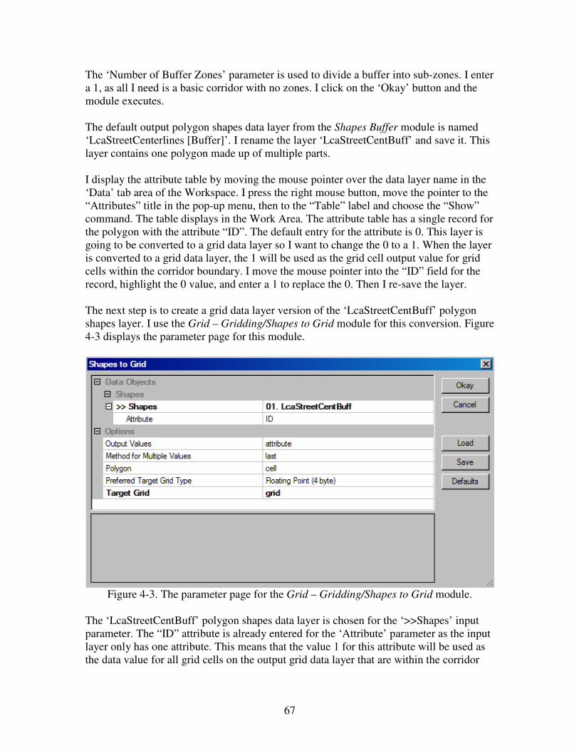
67
The ‘Number of Buffer Zones’ parameter is used to divide a buffer into sub-zones. I enter
a 1, as all I need is a basic corridor with no zones. I click on the ‘Okay’ button and the
module executes.
The default output polygon shapes data layer from the Shapes Buffer module is named
‘LcaStreetCenterlines [Buffer]’. I rename the layer ‘LcaStreetCentBuff’ and save it. This
layer contains one polygon made up of multiple parts.
I display the attribute table by moving the mouse pointer over the data layer name in the
‘Data’ tab area of the Workspace. I press the right mouse button, move the pointer to the
“Attributes” title in the pop-up menu, then to the “Table” label and choose the “Show”
command. The table displays in the Work Area. The attribute table has a single record for
the polygon with the attribute “ID”. The default entry for the attribute is 0. This layer is
going to be converted to a grid data layer so I want to change the 0 to a 1. When the layer
is converted to a grid data layer, the 1 will be used as the grid cell output value for grid
cells within the corridor boundary. I move the mouse pointer into the “ID” field for the
record, highlight the 0 value, and enter a 1 to replace the 0. Then I re-save the layer.
The next step is to create a grid data layer version of the ‘LcaStreetCentBuff’ polygon
shapes layer. I use the Grid – Gridding/Shapes to Grid module for this conversion. Figure
4-3 displays the parameter page for this module.
Figure 4-3. The parameter page for the Grid – Gridding/Shapes to Grid module.
The ‘LcaStreetCentBuff’ polygon shapes data layer is chosen for the ‘>>Shapes’ input
parameter. The “ID” attribute is already entered for the ‘Attribute’ parameter as the input
layer only has one attribute. This means that the value 1 for this attribute will be used as
the data value for all grid cells on the output grid data layer that are within the corridor
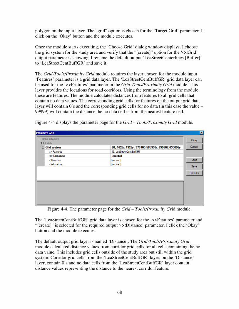
68
polygon on the input layer. The “grid” option is chosen for the ‘Target Grid’ parameter. I
click on the ‘Okay’ button and the module executes.
Once the module starts executing, the ‘Choose Grid’ dialog window displays. I choose
the grid system for the study area and verify that the “[create]” option for the ‘<<Grid’
output parameter is showing. I rename the default output ‘LcaStreetCenterlines [Buffer]’
to ‘LcaStreetCentBuffGR’ and save it.
The Grid-Tools/Proximity Grid module requires the layer chosen for the module input
‘Features’ parameter is a grid data layer. The ‘LcaStreetCentBuffGR’ grid data layer can
be used for the ‘>>Features’ parameter in the Grid-Tools/Proximity Grid module. This
layer provides the locations for road corridors. Using the terminology from the module
these are features. The module calculates distances from features to all grid cells that
contain no data values. The corresponding grid cells for features on the output grid data
layer will contain 0’s and the corresponding grid cells for no data (in this case the value –
99999) will contain the distance the no data cell is from the nearest feature cell.
Figure 4-4 displays the parameter page for the Grid – Tools/Proximity Grid module.
Figure 4-4. The parameter page for the Grid – Tools/Proximity Grid module.
The ‘LcaStreetCentBuffGR’ grid data layer is chosen for the ‘>>Features’ parameter and
“[create]” is selected for the required output ‘<<Distance’ parameter. I click the ‘Okay’
button and the module executes.
The default output grid layer is named ‘Distance’. The Grid-Tools/Proximity Grid
module calculated distance values from corridor grid cells for all cells containing the no
data value. This includes grid cells outside of the study area but still within the grid
system. Corridor grid cells from the ‘LcaStreetCentBuffGR’ layer, on the ‘Distance’
layer, contain 0’s and no data cells from the ‘LcaStreetCentBuffGR’ layer contain
distance values representing the distance to the nearest corridor feature.

69
I do not want the data values outside of the study area that contain data values to
contribute to the solution. I use the Grid-Tools/Grid Masking module to convert the
distance data outside of the study area to no data (-99999) values. Figure 4-5 displays the
parameter page for the Grid – Tools/Grid Masking module.
Figure 4-5. The ‘Grid Masking’ parameter page.
The default output layer from the Proximity Grid module, ‘Distance’, is chosen for the
input ‘>>Grid’ parameter and the “[create]” option for the ‘<Masked Grid’ output
parameter is entered. The grid data layer ‘LcaStudyAreaGR’ is chosen for the ‘>>Mask’
input parameter. I click the ‘Okay’ button and the module executes.
I rename the default output layer ‘Masked Grid’ to ‘LcaStreetCentBuffDistGR’ and save
it.
The data range for the ‘LcaStreetCentBuffDistGR’ layer is 0 to 14304.936523. On this
layer, values are distances grid cells are from corridor cells. The intent is to develop a
factor element cost layer that contains data values rescaled into continuous values
between 0 and 1 for the continuous data range from 0 to 14304.936523. Impacts from a
transmission line are lowest adjacent to existing corridors and increase with distance from
existing corridors. Thus the impact increases from 0 for cells adjacent to corridors to a
maximum of 1 for cells the furthest away.
The Grid – Calculus/Grid Normalisation module is used to rescale the data values on the
‘LcaStreetCentBuffDistGR’ layer. Figure 4-6 displays the parameter page for the Grid –
Calculus/Grid Normalisation module.
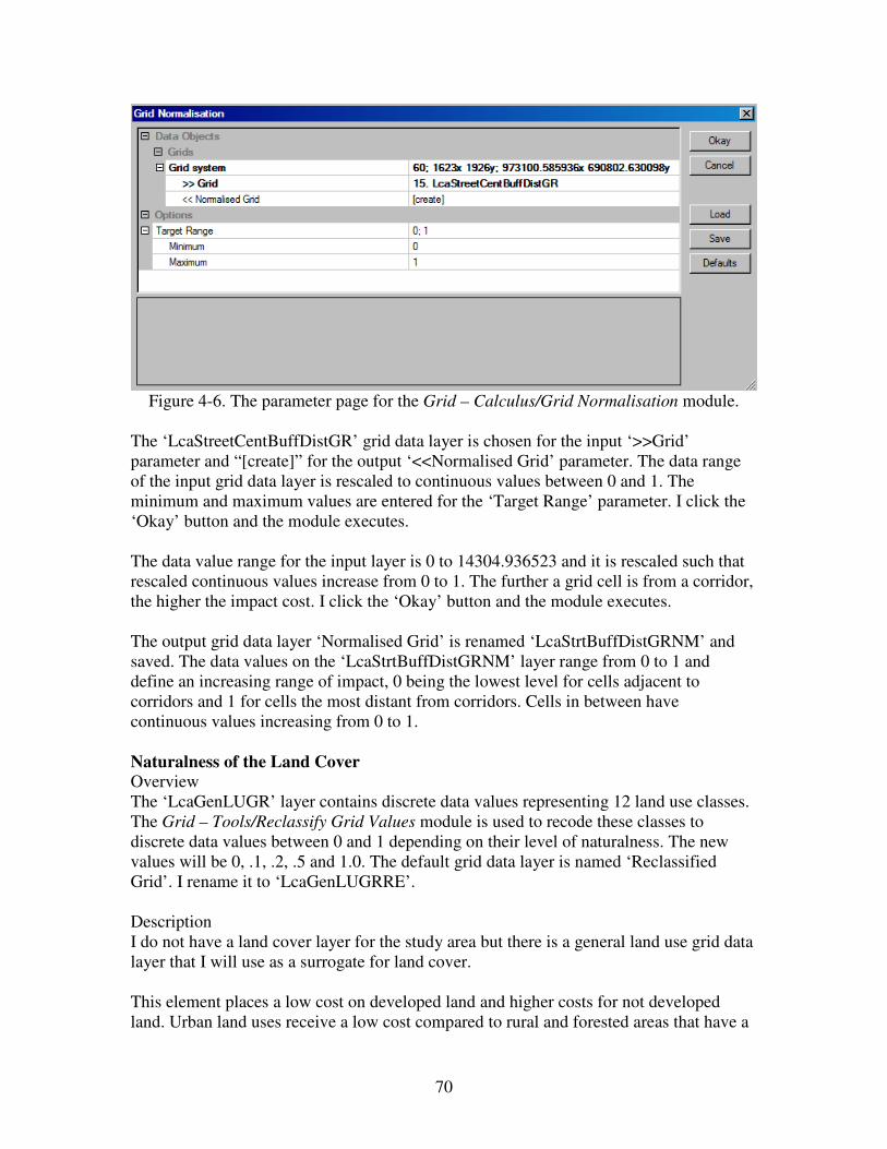
70
Figure 4-6. The parameter page for the Grid – Calculus/Grid Normalisation module.
The ‘LcaStreetCentBuffDistGR’ grid data layer is chosen for the input ‘>>Grid’
parameter and “[create]” for the output ‘<<Normalised Grid’ parameter. The data range
of the input grid data layer is rescaled to continuous values between 0 and 1. The
minimum and maximum values are entered for the ‘Target Range’ parameter. I click the
‘Okay’ button and the module executes.
The data value range for the input layer is 0 to 14304.936523 and it is rescaled such that
rescaled continuous values increase from 0 to 1. The further a grid cell is from a corridor,
the higher the impact cost. I click the ‘Okay’ button and the module executes.
The output grid data layer ‘Normalised Grid’ is renamed ‘LcaStrtBuffDistGRNM’ and
saved. The data values on the ‘LcaStrtBuffDistGRNM’ layer range from 0 to 1 and
define an increasing range of impact, 0 being the lowest level for cells adjacent to
corridors and 1 for cells the most distant from corridors. Cells in between have
continuous values increasing from 0 to 1.
Naturalness of the Land Cover
Overview
The ‘LcaGenLUGR’ layer contains discrete data values representing 12 land use classes.
The Grid – Tools/Reclassify Grid Values module is used to recode these classes to
discrete data values between 0 and 1 depending on their level of naturalness. The new
values will be 0, .1, .2, .5 and 1.0. The default grid data layer is named ‘Reclassified
Grid’. I rename it to ‘LcaGenLUGRRE’.
Description
I do not have a land cover layer for the study area but there is a general land use grid data
layer that I will use as a surrogate for land cover.
This element places a low cost on developed land and higher costs for not developed
land. Urban land uses receive a low cost compared to rural and forested areas that have a

71
high cost. The Grid – Tools/Reclassify Grid Values module is used to recode the
‘LcaGenLUGR’ land cover data values to the 0 to 1 data range.
There are 12 land use classes plus “none” on the ‘LcaGenLUGR’ grid data layer. The
“none” areas are mostly water and are recoded to 1. The table below displays the class
name, class data value, and a recode value.
Class Name Data Value Recode
None 0 1.0
Residential 1 .1
Industrial 2 .1
Transportation 3 .1
Utilities 4 .1
Commercial 5 .1
TELU 6 .1
Open Space 7 .5
Agriculture 8 .1
Forestry 9 1.0
Rural 10 .5
Mineral Extract 11 .2
Commercial Rec 12 .5
The “Recode” column shows the cost values within the 0 (low cost) to 1 (high cost) range
that will replace the class data values. Figure 4-7 displays the Grid – Tools/Reclassify
Grid Values module parameter page.
Figure 4-7. The Grid – Tools/Reclassify Grid Values module parameter page.

72
The ‘LcaGenLUGR’ grid data layer is chosen for the input parameter ‘>>Grid’ and
“[create]” is entered for the ‘<<Reclassified Grid’ output parameter. The “simple table”
option is chosen for the ‘Method’ parameter. Figure 4-8 displays the simple table
containing the values for recoding the data values.
Figure 4-8. The Grid – Tools/Reclassify Grid Values module ‘Lookup Table’ parameter
describing the recoding of the data values.
The current land use data values are listed in the “minimum” and “maximum” columns.
The new data values in the range from 0 to 1 are entered in the “new” column. As an
example, in row 2, land cover classes 1 through 6 are recoded to the value 0.1. Once I
enter the values for the lookup table, I click the ‘Okay’ button.
The “min <= value <= max” option is chosen for the ‘operator’ parameter. I am ready to
execute the module so I click the ‘Okay’ button on the Reclassify Grid Values module
parameter page.
I rename the default output grid data layer ‘Reclassified Grid” to ‘LcaGenLUGRRE’ and
save the new layer.
Distance From Ridge Buffers
Overview
1. A grid data layer for ridges or one for landforms that would include ridges does
not exist. I execute the Terrain Analysis – Morphometry/TPI Based Landform
Classification module to produce a landforms grid data layer. The input grid data
layer to the module is the study area DEM ‘LcaDEMfeetGR’. The default output
grid data layer is ‘Landforms’. I rename it to ‘LcaLandformsGR’.
2. The Grid – Calculus/Grid Calculator module uses the ‘LcaLandformsGR’ layer
as input to select the landform data value of 9 that represents “High Ridges”. High

73
ridge grid cells are output to a new grid data layer named ‘LcaRidgesTEMPGR’.
All non-ridge cells contain the no data value –99999.
3. The Grid – Tools/Grid Masking module is used to recode ridge data values
outside of the study area to the no data value –99999. The default output layer
‘Masked Grid’ is renamed ‘LcaRidgesGR’.
4. Prepare the ridge buffer width criteria layer using the Grid – Calculus/Grid
Calculator module. Input layers will be the ‘LcaRidgesTEMPGR’ and
‘LcaDEMfeetGR’ grid data layers. The output grid data layer is named
‘LcaRidgesBuffCritGR’.
5. Prepare a grid data layer of distances from ridges using the Grid –
Tools/Proximity Grid module. The input to the module is the ‘LcaRidgesGR’ grid
data layer. The default output layer is named ‘Distance’.
6. Use the Grid – Tools/Grid Masking module to convert distance data values
outside of the study area on the ‘Distance’ layer to no data values of –99999.
Name the default output ‘Masked Grid’ to ‘LcaBuffWidthGR’.
7. Create a data layer with variable width buffers around ridges using the Grid –
Tools/Threshold Buffer module. The input parameter ‘>>Features Grid’ will use
the ‘LcaRidgesGR’ layer; the input ‘>>Value Grid’ parameter will use the
‘LcaBuffWidthGR’ layer and the input ‘>Threshold Grid’ will use the
‘LcaRidgesBuffCritGR’ layer. The default output grid data layer is renamed
‘LcaRidgeBuffersTEMP’.
8. Apply the Grid Tools – Reclassify Grid Values module to recode the no data value
–2147483647 on the ‘LcaRidgeBuffersTEMP’ layer to –99999 and cells for
ridges and ridge buffers to 1’s. The default output grid data layer is named
‘Reclassified Grid’.
9. Data values outside of the study area on the ‘Reclassified Grid’ layer are changed
to no data values –99999 using the Grid – Tools/Grid Masking module. The
default output layer ‘Masked Grid’ is renamed to ‘LcaRidgeBuffRecGR’.
10. I use the Grid – Tools/Proximity Grid module to develop a layer with cells
containing distance values to ridge buffers. The input layer is the
‘LcaRidgeBuffRecGR’ layer. The default output grid data layer is named
‘Distance’ and renamed to ‘LcaRidgeBuffRecDistGR’.
11. The distance data values on the ‘LcaRidgeBuffRecDistGR’ are rescaled to the
data range 0 to 1. The Grid – Tools/Grid Normalisation module is used for this
task. The default output grid data layer ‘Normalised Grid’ is renamed
‘LcaRidgeBuffRecDistGRNM’.
Description
I do not have a data layer for ridges but I can use the SAGA Terrain Analysis –
Morphometry/TPI Based Landform Classification module to create a landform grid data
layer for the study area. One of the landform types on this layer is “High Ridges”. The
“High Ridges” landform uses the data value 9 on the landforms grid data layer.
Figure 4-9 displays the parameter page for the Terrain Analysis – Morphometry/TPI
Based Landform Classification module.

74
Figure 4-9. The Terrain Analysis – Morphometry/TPI Based Landform Classification
module parameter page.
The input for the ‘>>Elevation’ parameter is the ‘LcaDEMfeetGR’ grid data layer. This
is the digital elevation model for the study area. The “[create]” option is chosen for the
‘<<Landforms’ output parameter. The default output grid data layer is named
‘Landforms’. I click the ‘Okay’ button and the module executes. This module can take a
while to execute. I rename the default output layer to ‘LcaLandformsGR’ and save it.
The data value 9 on the ‘LcaLandformsGR’ grid data layer represents “High Ridges”. I
use the Grid – Calculus/Grid Calculator module to select all grid cells on the layer
containing the data value 9 and output them to a new grid data layer. I will output the no
data value –99999 to all non-ridge grid cells. I name the output ‘LcaRidgesGRTEMP’.
Figure 4-10 displays the parameter page for the Grid – Calculus/Grid Calculator module.
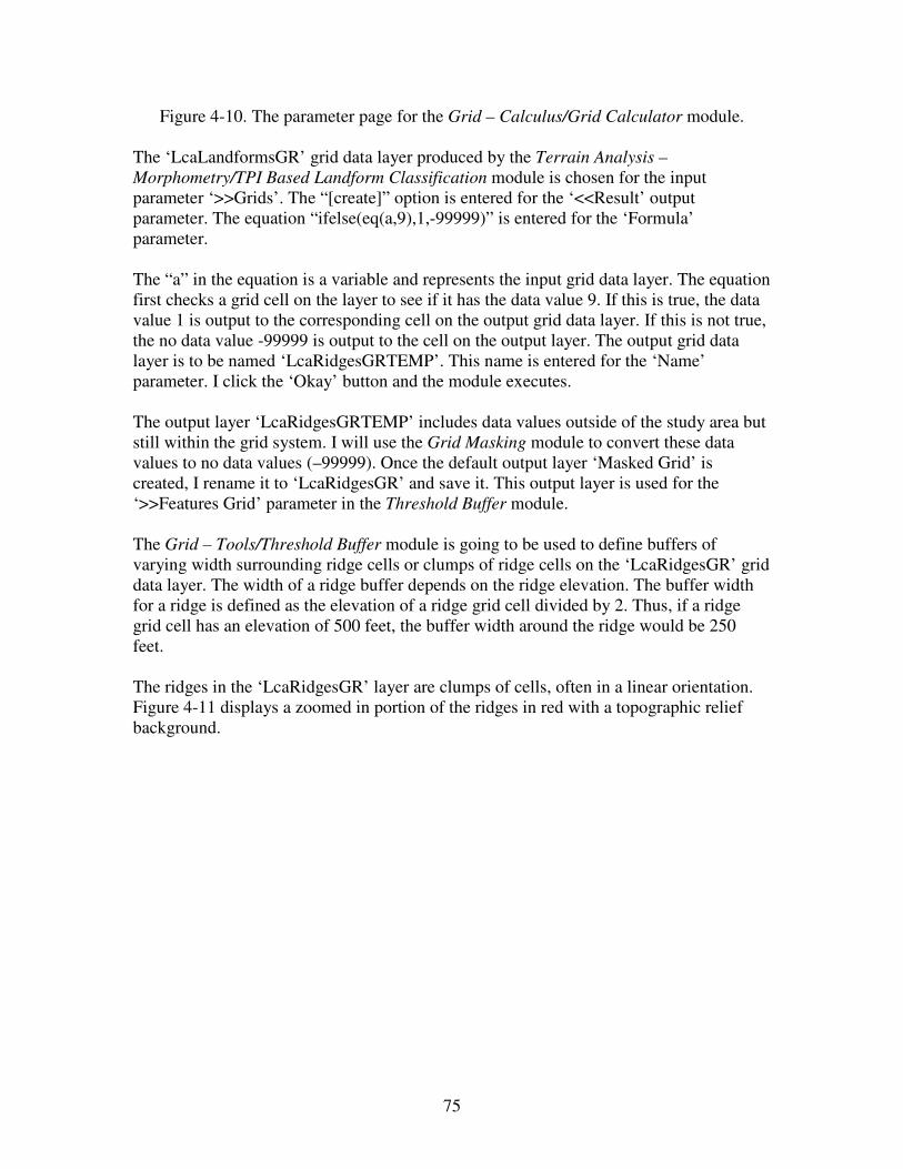
75
Figure 4-10. The parameter page for the Grid – Calculus/Grid Calculator module.
The ‘LcaLandformsGR’ grid data layer produced by the Terrain Analysis –
Morphometry/TPI Based Landform Classification module is chosen for the input
parameter ‘>>Grids’. The “[create]” option is entered for the ‘<<Result’ output
parameter. The equation “ifelse(eq(a,9),1,-99999)” is entered for the ‘Formula’
parameter.
The “a” in the equation is a variable and represents the input grid data layer. The equation
first checks a grid cell on the layer to see if it has the data value 9. If this is true, the data
value 1 is output to the corresponding cell on the output grid data layer. If this is not true,
the no data value -99999 is output to the cell on the output layer. The output grid data
layer is to be named ‘LcaRidgesGRTEMP’. This name is entered for the ‘Name’
parameter. I click the ‘Okay’ button and the module executes.
The output layer ‘LcaRidgesGRTEMP’ includes data values outside of the study area but
still within the grid system. I will use the Grid Masking module to convert these data
values to no data values (–99999). Once the default output layer ‘Masked Grid’ is
created, I rename it to ‘LcaRidgesGR’ and save it. This output layer is used for the
‘>>Features Grid’ parameter in the Threshold Buffer module.
The Grid – Tools/Threshold Buffer module is going to be used to define buffers of
varying width surrounding ridge cells or clumps of ridge cells on the ‘LcaRidgesGR’ grid
data layer. The width of a ridge buffer depends on the ridge elevation. The buffer width
for a ridge is defined as the elevation of a ridge grid cell divided by 2. Thus, if a ridge
grid cell has an elevation of 500 feet, the buffer width around the ridge would be 250
feet.
The ridges in the ‘LcaRidgesGR’ layer are clumps of cells, often in a linear orientation.
Figure 4-11 displays a zoomed in portion of the ridges in red with a topographic relief
background.
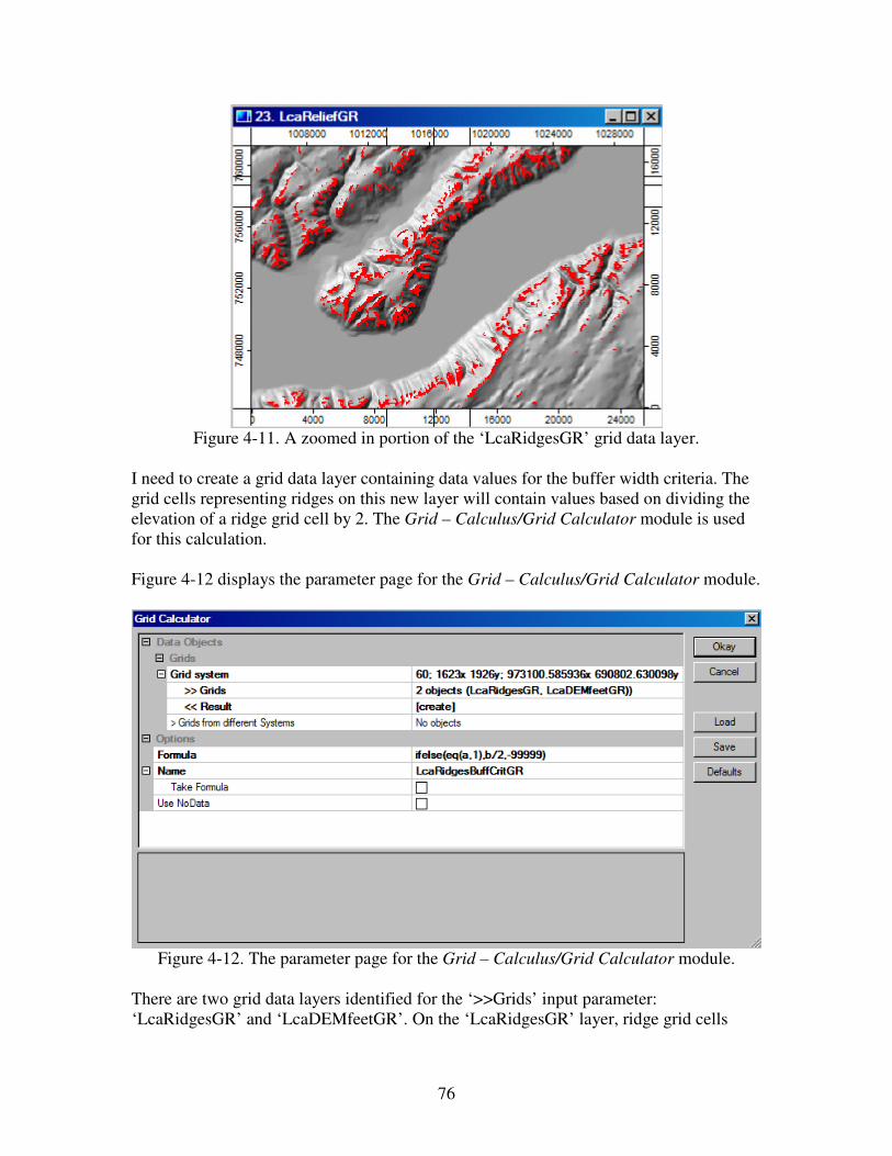
76
Figure 4-11. A zoomed in portion of the ‘LcaRidgesGR’ grid data layer.
I need to create a grid data layer containing data values for the buffer width criteria. The
grid cells representing ridges on this new layer will contain values based on dividing the
elevation of a ridge grid cell by 2. The Grid – Calculus/Grid Calculator module is used
for this calculation.
Figure 4-12 displays the parameter page for the Grid – Calculus/Grid Calculator module.
Figure 4-12. The parameter page for the Grid – Calculus/Grid Calculator module.
There are two grid data layers identified for the ‘>>Grids’ input parameter:
‘LcaRidgesGR’ and ‘LcaDEMfeetGR’. On the ‘LcaRidgesGR’ layer, ridge grid cells
77
have the data value 1. All other cells have the no data value –99999. The second layer is
the DEM for the study area. The grid cell values are the elevations of the cells.
The equation entered for the ‘Formula’ parameter is “ifelse(eq(a,1),b/2,-99999)”.
The equation entered for the ‘Formula’ parameter checks a grid cell value on the
‘LcaRidgesGR’ layer (represented in the equation by the variable “a”). If the cell value is
a 1 this means it is a cell that is a ridge or part of a ridge. In this case, the elevation value
in the corresponding cell on the ‘LcaDEMfeetGR’ layer (represented in the equation by
the variable “b”) is divided by 2 and the quotient is output to the corresponding cell on
the output layer. If the cell value is not a 1, then the no data value –99999 is output to the
output layer cell.
Please note that the last portion of the equation involving the no data value –99999 is
redundant. Recall that grid cells containing no data values on a layer, used in a
computation with other layers, the corresponding output cells will contain no data values.
Since all non-ridge grid cells on the ‘LcaRidgesGR’ layer contain no data values, the
output layer from the Grid Calculator will contain no data values for the same cells.
The name for the output layer is ‘LcaRidgesBuffCritGR’ and is entered for the ‘Name’
parameter. This layer is used for the ‘Threshold Grid’ parameter in the Threshold Buffer
module. The output layer is saved.
The Grid – Tools/Proximity Grid module is used to create a grid data layer with grid cells
containing distance values from ridges. The ‘LcaRidgesGR’ grid data layer is used for the
input ‘>>Features’ parameter. The module calculates distances from the ridge feature
grid cells to all no data cells in the layer. The corresponding grid cells for features on the
output grid data layer will contain 0’s and the corresponding grid cells for no data (in this
case the value –99999) will contain the distance the no data cell is from the nearest
feature cell. These distance values are used to implement the buffer width criterion for
ridges with the cell values on the ‘LcaRidgesBuffCritGR’ layer. The name of this layer
will be ‘LcaBuffWidthGR’. It will be used for the ‘>>Value Grid’ in the Threshold
Buffer module.
Figure 4-13 displays the parameter page for the Grid – Tools/Proximity Grid module.

78
Figure 4-13. The ‘Proximity Grid’ parameter page.
The ‘LcaRidgesGR’ grid data layer is chosen for the ‘>>Features’ parameter and
“[create]” is the option for the output parameter ‘<<Distance’. I click the’Okay’ button
and the module executes.
The output grid data layer is named ‘Distance’. The Grid-Tools/Proximity Grid module
calculated distance values from ridge grid cells to all cells containing the no data value.
This includes grid cells outside of the study area but still within the grid system. Ridge
grid cells from the ‘LcaRidgesGR’ layer, on the ‘Distance’ layer, contain 0’s and no data
cells from the ‘LcaRidgesGR’ layer contain distance values representing the distance to
the nearest ridge for the cell.
I do not want the data values outside of the study area that contain data values to
contribute to the solution. I use the Grid – Tools/Grid Masking module to convert those
values to no data values –99999 and rename the default ‘Masked Grid’ to
‘LcaBuffWidthGR’ and save it.
The three grid data layers that I need for the input parameters for the Grid –
Tools/Threshold Buffer module are now available. Figure 4-14 displays the parameter
page for the module.

79
Figure 4-14. The parameter page for the Grid – Tools/Threshold Buffer module.
The input for the ‘>>Features Grid’ parameter is the ‘LcaRidgesGR’ layer. Grid cells
representing ridges contain the data value 1. All other grid cell values are no data values
–99999. The input ‘Threshold Grid’ parameter grid data layer is ‘LcaRidgesBuffCritGR’.
The criterion for a ridge buffer width is that the buffer width is ½ the ridge elevation. The
ridge cell values on this layer are the quotient of dividing the elevation for the cell by 2.
All other cell values are no data values –99999. A ridge cell buffer width value is used to
find the distance from a ridge on the ‘LcaBuffWidthGR’ layer that is chosen for the
‘>>Value Grid’ \parameter. Cells with data values less than the cell value on the
‘LcaRidgesBuffCritGR’ are identified as ridge buffer cells until the buffer criterion value
is greater than the distance value. The two parameters in the ‘Options’ section are not
needed since a data layer is used to provide threshold data. I click the ‘Okay’ button and
the module executes. I rename the output data layer ‘LcaRidgeBuffersTEMP’.
As an example, let’s look at one ridge cell. The value for the ‘LcaRidgesGR’ layer cell is
1. All nearby cells contain the no data value of –99999. The elevation for the
corresponding cell on the ‘LcaDEMfeetGR’ layer is 300 feet. On the
‘LcaRidgesBuffCritGR’ layer the data value for the corresponding cell is 150. The buffer
width for a ridge is defined as ½ the elevation of the ridge cell. Dividing the elevation
values for ridges by 2 produced data values on the ‘LcaRidgesBuffCritGR’. The cells
adjacent to our one cell ridge on the ‘LcaBuffWidthGR’ were searched and the value 150
was compared to the distance values in cells around the ridge. All cells with a distance
value of less than 150 were identified and output as buffer cells for the one cell ridge.
Cells having a distance value greater than 150 do not meet the criteria for a buffer for the
ridge and were output as no data values, -99999.
One processing difference between the Grid – Tools/Threshold Buffer module and other
modules used for this tutorial is the no data value used. The Threshold Buffer module
‘Buffer’ output grid data layer uses a no data value of –2147483647. The other modules
used in this tutorial are using –99999. I want to be consistent so I use the Grid Tools –

80
Reclassify Grid Values module to recode –2147483647 to –99999. In addition, I also
want ridge grid cells and ridge buffer grid cells to contain 1’s and all other grid cells to be
no data cells. Figure 4-15 displays the parameter page for these two objectives.
Figure 4-15. The Grid Tools – Reclassify Grid Values module parameter page.
The grid data layer ‘LcaRidgeBuffersTEMP’ produced by the Threshold Buffer module is
chosen for the input ‘>>Grid’ parameter and the “[create]” option used for the output
‘<<Reclassified Grid’ parameter. The “simple table” option is chosen for the ‘Method’
parameter.
The lookup table contains two rows. The first row uses the current no data value, –
2147483647 as the minimum field and 0 for the maximum field. The new value is –
99999. The second row lists the value 1 for the minimum and 2 for the maximum and a
new value of 1. On the ‘LcaRidgeBuffersTEMP’ layer, ridges are defined by the data
value 2 and buffers use the data value 1. I click on the ‘Okay’ button and the module
executes.
The output ‘Reclassified Grid’ contains data values outside of the study area so I use the
Grid – Tools/Grid Masking module to convert the values to no data values –99999. I
rename the default output ‘Masked Grid’ to ‘LcaRidgeBuffRecGR’ and save it.
The next step is to use the ‘LcaRidgeBuffRecGR’ layer and the Grid – Tools/Proximity
Grid module to produce a grid data layer containing 0’s for ridge/ridge buffer cells and
distances from ridge/ridge buffers for all other cells. The ‘LcaRidgeBuffRecGR’ layer is
used for the ‘>>Features’ parameter in the Grid – Tools/Proximity Grid module. This
layer provides the locations for ridges/ridge buffers, i.e., features. The module calculates
distances from features to all grid cells that contain no data values. The corresponding
grid cells for features on the output grid data layer will contain 0’s and the corresponding

81
grid cells for no data (in this case the value –99999) will contain the distance the no data
cell is from the nearest feature cell.
Figure 4-16 displays the parameter page for the Grid – Tools/Proximity Grid module.
Figure 4-16. The Grid – Tools/Proximity Grid module parameter page.
The ‘LcaRidgebuffRecGR’ layer is chosen for the ‘>>Features’ parameter. The “[create]”
option is entered for the ‘<<Distance’ output parameter. I click the ‘Okay’ button to
execute the module.
The default output grid data layer is named ‘Distance’. The Grid-Tools/Proximity Grid
module calculated distance values from ridges/ridge buffer grid cells to all cells
containing the no data value. The ‘Distance’ grid data layer contains distance values
outside of the study area. I use the Grid – Tools/Grid Masking module to convert the data
values outside of the study area to no data values –99999. The default output ‘Masked
Grid’ from the Grid Masking module is renamed to ‘LcaRidgeBuffRecDistGR’ and
saved.
The data range for the ‘LcaRidgeBuffRecDistGR’ layer is 0 to 6832.627441. On this
layer, values are distances grid cells are from the nearest ridge buffer. The intent is to
develop a factor element cost layer that contains data values rescaled into continuous
values between 0 and 1 for the continuous data range from 0 to 6832.627441. Because
impacts are higher the closer a transmission line is to a ridge buffer, the continuous data
range from 0 to 1 defines impacts from high (close to a ridge buffer) to low, the further a
cell is from a ridge buffer.
The Grid – Calculus/Grid Normalisation module is used to rescale the data values on the
‘LcaRidgeBuffRecDistGR’ layer. Figure 4-17 displays the parameter page for the Grid –
Calculus/Grid Normalisation module.

82
Figure 4-17. The parameter page for the Grid – Tools/Grid Normalisation module.
The ‘LcaRidgeBuffRecDistGR’ grid data layer is chosen for the input ‘>>Grid’
parameter and “[create]” for the output ‘<<Normalised Grid’ parameter. The data range
of the input grid data layer is rescaled to continuous values between 0 and 1. The
minimum and maximum values are entered for the ‘Target Range’ parameter. I click the
‘Okay’ button and the module executes.
This is one of the factor elements where the existing data range of continuous values is
inversely rescaled to valued between 1 and 0. The data value range for the input layer is 0
to 6832.627441 and it is rescaled such that rescaled continuous values decrease from 1
for 0 to 0 for 6832.627441. This is because the nearer the grid cell is to a ridge buffer, the
higher the impact cost.
The output grid data layer ‘Normalised Grid’ is renamed ‘LcaRidgeBuffRecDistGRNM’
and saved. The data values on the ‘LcaRidgeBuffRecDistGRNM’ layer range from 0 to 1
and define an increasing range of impact, 1 being the highest level for cells adjacent to
ridge buffers and 0 for cells the most distant from ridge buffers. Cells in between have
values decreasing from 1 to 0.
The Natural Model Least Cost Path
Overview
1. Apply the importance weight to each element grid data layer and combine the
weighted element layers into a single cost surface layer using the Grid – Calculus/Grid
Calculator module. Name the combined layer ‘LcaCostNatrModGR’.
2. Use the combined element cost surface layer for the model (the ‘LcaCostNatrModGR’
layer) and the ‘LcaDestinationPointGR’ grid data layer for the destination substation as
inputs to the Grid – Analysis/Accumulated Cost (Isotropic) module and create the
accumulated cost grid data layer. Name the accumulated cost grid data layer
‘LcaAccumNatrModGR’.
3. The point shapes data layer for the source substation (‘LcaSourcePoint’) and the
accumulated cost grid data layer, ‘LcaAccumNatrModGR’, are inputs to the Grid –

83
Analysis/Least Cost Paths module for calculating the least cost path solution for the
model. The default shapes outputs ‘Profile_Line_[LcaAccumNatrModGR]_3’) and
‘Profile_Points_[LcaAccumNatrModGR]_3’ are renamed to ‘LcaLCPlineMod3’ and
‘LcaLCPApointsMod3’.
Description
The four factor elements of the determinant model have now been prepared and are ready
to be combined using the factor element importance weights and the Grid-Calculus/Grid
Calculator module. The determinant model elements and their weights are displayed
below.
Aspect (.15)
Distance From Infrastucture Corridors (.35)
Naturalness of the Land Cover (.35)
Distance From Ridge Buffers (.15)
The numbers in parentheses are impact weights and total to 1.0. Seventy percent of the
impact for this model is accounted for with the two elements “Distance From
Infrastructure Corridors” and “Naturalness of the Land Cover”. The other two elements
each have an impact weight of .15.
The Grid-Calculus/Grid Calculator module is used to apply the weights to the layers and
add the layers together in a single execution of the module. Figure 4-18 displays the
parameter page for the Grid-Calculus/Grid Calculator module.
Figure 4-18. The parameter page for the Grid-Calculus/Grid Calculator module.
The input parameter ‘>>Grids’ value field is where the names of the four element grid
data layers of the model are entered. The grid data layers for the four elements are
‘LcaAspectDegGRFUZ’, ‘LcaStrtBuffDistGRNM’, ‘LcaGenLUGRRE’, and
‘LcaRidgeBuffRecDistGRNM’.
The equation entered for the ‘Formula’ parameter is “(a*.15)+(b*.35)+(c*.35)+(d*.15)”.

84
The variables a, b, c and d in the equation represent the four grid data layers in the input
parameter value field in the order they appear. The values .15, .35, .35 and .15 are the
layer importance weights. The weight for a layer is multiplied times the data values in the
layer grid cells. The resultants for corresponding grid cells on other layers are added
together and output to the corresponding grid cell of the output grid data layer named
‘LcaCostNatrModGR’. The output layer is saved. This is the cost surface layer for the
model.
The cost surface layer ‘LcaCostNatrModGR’ and the ‘LcaDestinationPointGR’ layer are
the input layers to the Grid – Analysis/Accumulated Cost (Isotropic) module. The default
output layer ‘Accumulated Cost’ from this module contains cumulative cost data values
increasing in value radiating out from the single destination point grid cell on the
‘LcaDestinationPointGR’ layer. The more distant you go from the zero point the more
cost is accumulated in a grid cell. Figure 4-19 displays the parameter page for the Grid –
Analysis/Accumulated Cost (Isotropic) module.
Figure 4-19. The parameter page for the Grid – Analysis/Accumulated Cost (Isotropic)
module.
The ‘LcaCostNatrModGR’ and ‘LcaDestinationPointGR’ grid data layers are chosen for
the input parameters ‘>>Cost Grid’ and ‘>>Destination Points’. The “[create]” option is
the default for the two output parameters and is automatically entered for them. I am only
interested in the output layer accumulated cost. Its’ default name is ‘Accumulated Cost’. I
rename the output ‘Accumulated Cost’ layer to ‘LcaAccumNatrModGR’ and save it. The
output for the closest point will not be used.
The Grid – Analysis/Least Cost Paths module is used to locate the least cost path
between the destination grid cell (that is the only cell with a 0 value on the
‘LcaAccumNatrModGR’ layer) and a source point that is defined in the point shapes data
layer named ‘LcaSourcePoint’. The destination point is the substation located in the
northern half of the study area and the source point is the station in the southwest

85
quadrant. Figure 4-20 displays the parameter page for the Grid – Analysis/Least Cost
Paths module.
Figure 4-20. The ‘Least Cost Paths’ parameter page.
The grid data layer ‘LcaAccumNatrModGR’ is chosen for the input ‘>>Accumulated
cost’ parameter. The ‘LcaAccumNatrModGR’ layer is the output layer from the Grid –
Analysis/Accumulated Cost (Isotropic) module. The point shapes data layer
‘LcaSourcePoint’ is chosen for the ‘>>Source Point(s)’ input parameter. This layer
contains the point object for the substation located in the southwest quadrant of the study
area. I click on the ‘Okay’ button and the module executes.
The Grid – Analysis/Least Cost Paths module produces two shapes layers; one is a point
shapes data layer (default name ‘Profile_Line_[LcaAccumNatrModGR]_1’) and the other
is a line shapes data layer (default name ‘Profile_Points_[LcaAccumNatrModGR]_1’).
The point shapes data layer has point objects defining the location of the least cost path
between the two points. There is one point object for each grid cell the least cost path
traverses. The line shapes data layer has a line defining the location of the least cost path
between the two points. I rename the default output layers to ‘LcaLCPAlineMod3’ and
‘LcaLCPpointsMod3’ and save both of them.
Figure 4-21 displays the least cost path solution for this model using the color aqua.

86
Figure 4-21. The least cost path solution for the human health determinant model.
The two substations are shown in Figure 4-20 with red circles. The substation to the north
of the large body of water (the south end of Hood Canal) is the destination. The
substation in the southwest quadrant of the display is the source. The road network for the
study area is displayed in black and the background is the topographic relief in shades of
gray. Water areas are filled with blue.
The aqua colored line connecting the two substations is the least cost path solution for the
natural determinant model. The least cost path solutions for the other two models are also
shown, in green for the human health model and maroon for the landscape model.
5. Two “Composite” Least Cost Path Solutions
I will look at two solutions that combine the three models using different sets of model
importance weights. The first composite is where each model has equal weight toward
the solution. The list below displays the model name, the importance weight, and the cost
surface grid data layer name.
The Equal Weight Composite
Model Name Weight Cost Surface Layer
The Human Health Model .333 LcaCostHthModGR
Landscape Model .333 LcaCostLandModGR
Nature .333 LcaCostNatrModGR
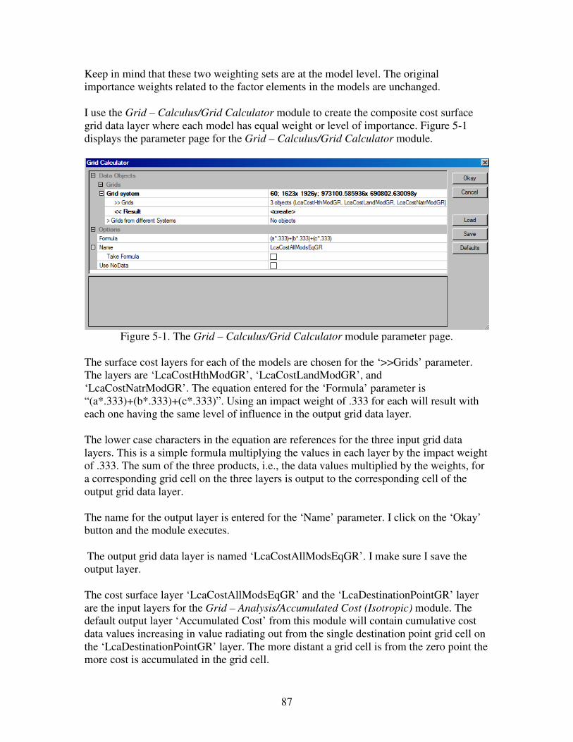
87
Keep in mind that these two weighting sets are at the model level. The original
importance weights related to the factor elements in the models are unchanged.
I use the Grid – Calculus/Grid Calculator module to create the composite cost surface
grid data layer where each model has equal weight or level of importance. Figure 5-1
displays the parameter page for the Grid – Calculus/Grid Calculator module.
Figure 5-1. The Grid – Calculus/Grid Calculator module parameter page.
The surface cost layers for each of the models are chosen for the ‘>>Grids’ parameter.
The layers are ‘LcaCostHthModGR’, ‘LcaCostLandModGR’, and
‘LcaCostNatrModGR’. The equation entered for the ‘Formula’ parameter is
“(a*.333)+(b*.333)+(c*.333)”. Using an impact weight of .333 for each will result with
each one having the same level of influence in the output grid data layer.
The lower case characters in the equation are references for the three input grid data
layers. This is a simple formula multiplying the values in each layer by the impact weight
of .333. The sum of the three products, i.e., the data values multiplied by the weights, for
a corresponding grid cell on the three layers is output to the corresponding cell of the
output grid data layer.
The name for the output layer is entered for the ‘Name’ parameter. I click on the ‘Okay’
button and the module executes.
The output grid data layer is named ‘LcaCostAllModsEqGR’. I make sure I save the
output layer.
The cost surface layer ‘LcaCostAllModsEqGR’ and the ‘LcaDestinationPointGR’ layer
are the input layers for the Grid – Analysis/Accumulated Cost (Isotropic) module. The
default output layer ‘Accumulated Cost’ from this module will contain cumulative cost
data values increasing in value radiating out from the single destination point grid cell on
the ‘LcaDestinationPointGR’ layer. The more distant a grid cell is from the zero point the
more cost is accumulated in the grid cell.

88
Figure 5-2 displays the parameter page for the Grid – Analysis/Accumulated Cost
(Isotropic) module.
Figure 5-2. The parameter page for the Grid – Analysis/Accumulated Cost (Isotropic)
module.
The ‘LcaCostAllModsEqGR’ grid data layer is chosen for the ‘>>Cost Grid’ parameter
and the ‘LcaDestinationPointGR’ layer for the other input parameter ‘>>Destination
Points’. The default entry for the output parameter ‘<<Accumulated Cost’ is “[create]”. I
click on the ‘Okay’ button and the model executes. I rename the output grid data layer to
‘LcaAccumAllModsEqGR’ and save it.
Figure 5-3 displays the parameter page for the Grid – Analysis/Least Cost Paths module.
Figure 5-3. The Grid – Analysis/Least Cost Paths module parameter page.

89
The accumulated cost grid data layer produced by the Grid – Analysis/Accumulated Cost
(Isotropic) module, ‘LcaAccumAllModsEqGR’, is chosen for the input parameter
‘>>Accumulated cost’. The input for the shapes data layer parameter ‘>>Source Point(s)’
is ‘LcaSourcePoint’. This layer contains the point object for the substation located in the
southwest quadrant of the study area. This module will produce two shapes layers; one is
a point shapes data layer (default name ‘Profile_Line_[LcaAccumAllModsEqGR]_1’)
and the other is a line shapes data layer (default name
‘Profile_Points_[LcaAccumAllModsEqGR]_1’). The point shapes data layer has point
objects defining the location of the least cost path between the two points. The line
shapes data layer has a line defining the location of the least cost path between the two
points. I click on the ‘Okay’ button and the module executes.
The two output shapes data layers will be renamed ‘LcaLCPALineModsEq’ and
‘LcaLCPAPointsModsEq’ and saved.
Figure 5-4. The least cost path solution in red for each model equally weighted.
The two substations are shown in Figure 5-4 with red circles. The substation to the north
of the large body of water (the south end of Hood Canal) is the destination. The
substation in the southwest quadrant of the display is the source. The road network for the
study area is displayed in black and the background is the topographic relief in shades of
gray. Water areas are filled with blue.
The red line on the graphic in Figure 5-4 represents the least cost path solution when the
three models are weighted equally. The aqua colored line connecting the two substations
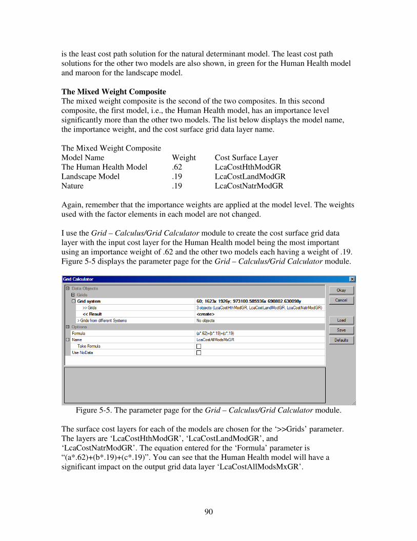
90
is the least cost path solution for the natural determinant model. The least cost path
solutions for the other two models are also shown, in green for the Human Health model
and maroon for the landscape model.
The Mixed Weight Composite
The mixed weight composite is the second of the two composites. In this second
composite, the first model, i.e., the Human Health model, has an importance level
significantly more than the other two models. The list below displays the model name,
the importance weight, and the cost surface grid data layer name.
The Mixed Weight Composite
Model Name Weight Cost Surface Layer
The Human Health Model .62 LcaCostHthModGR
Landscape Model .19 LcaCostLandModGR
Nature .19 LcaCostNatrModGR
Again, remember that the importance weights are applied at the model level. The weights
used with the factor elements in each model are not changed.
I use the Grid – Calculus/Grid Calculator module to create the cost surface grid data
layer with the input cost layer for the Human Health model being the most important
using an importance weight of .62 and the other two models each having a weight of .19.
Figure 5-5 displays the parameter page for the Grid – Calculus/Grid Calculator module.
Figure 5-5. The parameter page for the Grid – Calculus/Grid Calculator module.
The surface cost layers for each of the models are chosen for the ‘>>Grids’ parameter.
The layers are ‘LcaCostHthModGR’, ‘LcaCostLandModGR’, and
‘LcaCostNatrModGR’. The equation entered for the ‘Formula’ parameter is
“(a*.62)+(b*.19)+(c*.19)”. You can see that the Human Health model will have a
significant impact on the output grid data layer ‘LcaCostAllModsMxGR’.

91
The lower case characters in the equation are references for the three input grid data
layers. This is a simple formula multiplying the values on each layer by the impact
weight .62 for the human health model layer and .19 for each of the landscape and nature
model layers. The sum of the three products, i.e., the data values multiplied by the
weights, for a corresponding grid cell on the three layers is output to the corresponding
cell of the output grid data layer.
The name for the output layer is entered for the ‘Name’ parameter. I click on the ‘Okay’
button and the model executes. I save the output grid data layer
‘LcaCostAllModsMxGR’.
The cost surface layer ‘LcaCostAllModsMxGR’ and the ‘LcaDestinationPointGR’ layer
are the input layers for the Grid – Analysis/Accumulated Cost (Isotropic) module. The
default output layer ‘Accumulated Cost’ from this module will contain cumulative cost
data values increasing in value radiating out from the single destination point grid cell on
the ‘LcaDestinationPointGR’ layer. The more distant a grid cell is from the zero point the
more cost is accumulated in the grid cell. Figure 5-6 displays the parameter page for the
Grid – Analysis/Accumulated Cost (Isotropic) module.
Figure 5-6. The parameter page for the Grid – Analysis/Accumulated Cost (Isotropic)
module.
The ‘LcaCostAllModsMxGR’ grid data layer is chosen for the ‘>>Cost Grid’ parameter
and the ‘LcaDestinationPointGR’ layer for the other input parameter ‘>>Destination
Points’. The default entry for the output parameter ‘<<Accumulated Cost’ is “[create]”. I
click on the ‘Okay’ button and the module executes. I rename the default output grid data
layer ‘Accumulated Cost’ to ‘LcaAccumAllModsMxGR’ and save it.
Figure 5-7 displays the parameter page for the Grid – Analysis/Least Cost Paths module.

92
Figure 5-7. The parameter page for the Grid – Analysis/Least Cost Paths module.
The accumulated cost grid data layer produced by the Grid – Analysis/Accumulated Cost
(Isotropic) module, ‘LcaAccumAllModsMxGR’, is chosen for the input parameter
‘>>Accumulated cost’. The input for the shapes data layer parameter ‘>>Source Point(s)’
is ‘LcaSourcePoint’. This layer contains the point object for the substation located in the
southwest quadrant of the study area. This module will produce two shapes layers; one is
a point shapes data layer (default name ‘Profile_Line_[LcaAccumAllModsMxGR]_1’)
and the other is a line shapes data layer (default name
‘Profile_Points_[LcaAccumAllModsMxGR]_1’). The point shapes data layer has point
objects defining the location of the least cost path between the two points. The line
shapes data layer has a line defining the location of the least cost path between the two
points. The two output shapes data layers will be renamed ‘LcaLCPALineModsMx’ and
‘LcaLCPAPointsModsMx’.

93
Figure 5-8. The least cost path solution in yellow where the human health model is
significantly more important in weighting.
The two substations are shown in Figure 5-8 with red circles. The substation to the north
of the large body of water (the south end of Hood Canal) is the destination. The
substation in the southwest quadrant of the display is the source. The road network for the
study area is displayed in black and the background is the topographic relief in shades of
gray. Water areas are filled with blue.
The yellow line on the graphic in Figure 5-8 represents the least cost path solution for the
mixed weighted models. The red line represents the least cost path solution when the
three models are weighted equally. The aqua colored line connecting the two substations
is the least cost path solution for the natural determinant model. The least cost path
solutions for the other two models are also shown, in green for the human health model
and maroon for the landscape model.
6. Analysis
This last section introduces tools in SAGA that can be used to support making
comparisons on how the five least cost path solutions developed in this tutorial affect
various physical and cultural features in the study area. I am going to base the
comparisons on a 600’ right-of-way (ROW) for each line, i.e., 300’ on each side of the
line.
94
I am using a spreadsheet program, Excel, to create the various tabular displays. The
modules I use for generating statistics for length or area produce these metrics in feet and
square feet. My data summaries display length in miles and square feet in acres. Much of
the module output that I rely on is in linear feet or square feet. It is relatively easy, using
Excel functions, to convert module output using 5280 feet per mile, 42560 square feet per
acre, or, in the case of my study area grid system, 48.4 grid cells per acre. Can the same
conversions be done in SAGA? Yes, they can. They are easier to do, for me, in Excel and
Excel also has features making it easy to design tables, move rows and columns, etc.
This section will present comparisons related to five evaluation criteria. Here are the titles
for the evaluations in this section.
Line – ROW Statistics
Impact on South-Facing Aspects and Slope Gradients
Number of Residential Structures Within the Corridors
Comparing Estimated Market Value or ROW Property
Comparing Land Use Class Differences
I need both vector or polygon shapes data layer and a grid data layer version for each of
the five line shape data layers for the least cost path solutions. Here is a list of the line
shape data layers and their description.
Layer Name Description
‘LcaLCPALineMod1’ The Human Health model solution
‘LcaLCPALineMod2’ The Landscape model solution
‘LcaLCPALineMod3’ The Nature model solution
‘LcaLCPALineModsEq’ The equal weighted model composite solution
‘LcaLCPALineModsMx’ The mixed weighted model composite solution
I use the Shapes – Tools/Shapes Buffer module to develop a polygon shapes data layer for
each line representing the lines 600’ ROW. A grid data layer version of each polygon
shapes data layer is created using the Grid – Gridding/Shapes to Grid module. The
polygon shapes data layer created by the Shapes Buffer module is input for the Shapes to
Grid module.
Figure 6-1 displays the parameter page for the Shapes – Tools/Shapes Buffer module.

95
Figure 6-1. The ‘Shapes Buffer’ parameter page.
The parameters entered for executing this module will produce a 600’ buffer (ROW)
around the line object in the ‘LcaLCPALineMod1’ line shapes data layer. This layer is
chosen for the ‘>>Shapes’ input parameter. The entry for the ‘Buffer Distance’ parameter
is “constant”. The other choice is “attribute”. The ROW width of 300’ is constant for the
entire line and means that a 300’ buffer is defined on each side of the line. Since that is
the case, the “constant” option is used. The ‘Dissolve Buffers’ parameter check box
contains a check. This is the default. I leave the default, as it will not make any difference
because only one polygon is going to be created. I do not want zones within the ROW so
the default 1 is left for the ‘Number of Buffer Zones’ parameter. I click the ‘Okay’ button
and the module executes.
The default output polygon shapes data layer is named ‘LcaLCPALineMod1 [Buffer]’. I
rename the default output to ‘LcaLCPAMod1corr’ and save it.
I now create the grid data layer version of the ‘LcaLCPAMod1corr’ polygon shapes data
layer. Figure 6-2 displays the parameter page for the Grid – Gridding/Shapes to Grid
module.

96
Figure 6-2. The parameter page for the Grid – Gridding/Shapes to Grid module.
The polygon shapes data layer produced by the Shapes – Tools/Shapes Buffer module,
‘LcaLCPAMod1corr’, is chosen for the ‘>>Shapes’ parameter. The attribute table has a
single attribute and one record for the one polygon object in the layer. The value for the
attribute for the single polygon object is 0. There are two options for the ‘Target Grid’
parameter: “user defined” and “grid”. I choose the “grid” option because I want the
output grid data layer to be a member of the study area grid system. I click on the ‘Okay’
button and the module executes.
When the dialog window ‘Choose Grid’ displays during module execution I choose the
study area grid system and verify that the “[create]” option for the ‘<<Grid’ output
parameter is showing. The default name for the output grid data layer is
‘LcaLCPAMod1corr [ID]’. I rename it ‘LcaLCPAMod1corrGR’ and save it.
I execute the two modules described above for each of the five least cost path solutions.
The list of the new corridor related data layers is below.
Line Corridor Corridor
Line Shapes Data Layer Polygon Shapes Data Layer Grid Data Layer
‘LcaLCPALineMod1’ ‘LcaLCPAMod1corr’ ‘LcaLCPAMod1corrGR’
‘LcaLCPALineMod2’ ‘LcaLCPAMod2corr’ ‘LcaLCPAMod2corrGR’
‘LcaLCPALineMod3’ ‘LcaLCPAMod3corr’ ‘LcaLCPAMod3corrGR’
‘LcaLCPALineModsEq’ ‘LcaLCPAModEqcorr’ ‘LcaLCPAModEqcorrGR’
‘LcaLCPALineModsMx’ ‘LcaLCPAModMxcorr’ ‘LcaLCPAModMxcorrGR’
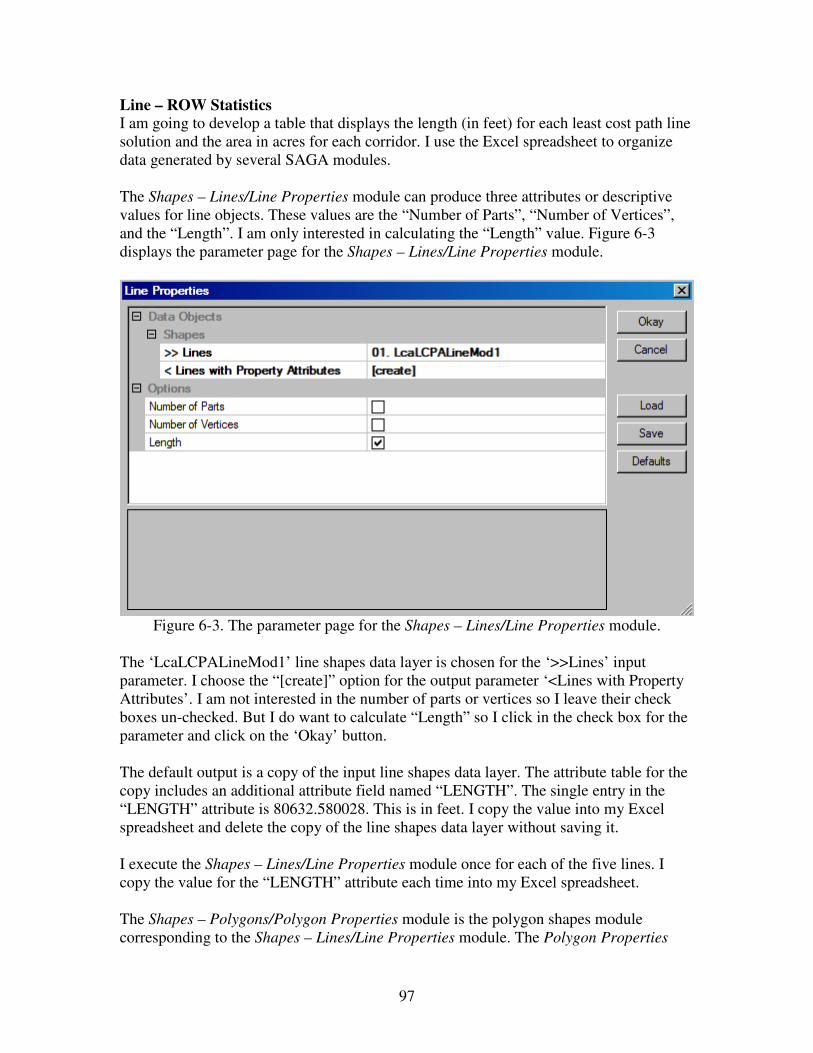
97
Line – ROW Statistics
I am going to develop a table that displays the length (in feet) for each least cost path line
solution and the area in acres for each corridor. I use the Excel spreadsheet to organize
data generated by several SAGA modules.
The Shapes – Lines/Line Properties module can produce three attributes or descriptive
values for line objects. These values are the “Number of Parts”, “Number of Vertices”,
and the “Length”. I am only interested in calculating the “Length” value. Figure 6-3
displays the parameter page for the Shapes – Lines/Line Properties module.
Figure 6-3. The parameter page for the Shapes – Lines/Line Properties module.
The ‘LcaLCPALineMod1’ line shapes data layer is chosen for the ‘>>Lines’ input
parameter. I choose the “[create]” option for the output parameter ‘<Lines with Property
Attributes’. I am not interested in the number of parts or vertices so I leave their check
boxes un-checked. But I do want to calculate “Length” so I click in the check box for the
parameter and click on the ‘Okay’ button.
The default output is a copy of the input line shapes data layer. The attribute table for the
copy includes an additional attribute field named “LENGTH”. The single entry in the
“LENGTH” attribute is 80632.580028. This is in feet. I copy the value into my Excel
spreadsheet and delete the copy of the line shapes data layer without saving it.
I execute the Shapes – Lines/Line Properties module once for each of the five lines. I
copy the value for the “LENGTH” attribute each time into my Excel spreadsheet.
The Shapes – Polygons/Polygon Properties module is the polygon shapes module
corresponding to the Shapes – Lines/Line Properties module. The Polygon Properties

98
module produces four attributes or descriptive values for polygon objects. These values
are the “Number of Parts”, “Number of Vertices”, “Perimeter” and the “Area”. I am only
interested in calculating the “Area” value. Figure 6-4 displays the parameter page for the
Shapes – Polygons/Polygon Properties module.
Figure 6-4. The ‘Polygon Properties’ parameter page.
The ‘LcaLCPAMod1corr’ polygon shapes data layer is chosen for the ‘>>Polygons’
input parameter. I choose the “[create]” option for the output parameter ‘<Polygons’ with
Property Attributes’. I am not interested in the number of parts or vertices or perimeter so
I leave their check boxes un-checked. But I do want to calculate “Area” so I click in the
check box for the parameter and click on the ‘Okay’ button.
The default output is a copy of the input line shapes data layer. The attribute table for the
copy includes an additional attribute field named “AREA”. The single entry in the
“AREA” attribute is 48530289.454960. This is in square feet. I copy the value into my
Excel spreadsheet and delete the copy of the polygon shapes data layer without saving it.
I execute the Shapes – Lines/Polygon Properties module once for each of the five lines.
Entering the value for the “AREA” attribute each time into my Excel spreadsheet.

99
Here are the summary statistics for the five least cost path line solutions.
Line Corridor
Feet Miles Square Ft Acres
Human Health Model 80632.58 15.27 48530289.45 1114.10
Landscape Model 80408.90 15.23 48425647.29 1111.70
Nature Model 102155.52 19.35 60825187.86 1396.35
Models Equally Weighted 82484.57 15.62 49503835.02 1136.45
Models Mixed Weights 80955.67 15.33 48689876.25 1117.77
Figure 6-5. Summary statistics for the five least cost path line solutions.
Impact on South-Facing Aspects and Slope Gradient
South-facing slope is a factor element in the Nature model. In addition to using south-
facing slope, I am using slope gradient as an evaluation criterion for comparing the line
solutions.
I use the Grid – Tools/Reclassify Grid Values module to recode continuous values on the
‘LcaAspectDegGR’ grid data layer to a layer containing four discrete data categories.
Figure 6-6 displays the parameter page for the Grid – Tools/Reclassify Grid Values
module.
Figure 6-6. The Grid – Tools/Reclassify Grid Values module parameter page.
The ‘LcaAspectDegGR’ grid data layer is chosen for the ‘>>Grid’ parameter and
“[create]” for the output parameter ‘<<Reclassified Grid’. The output layer is going to
contain four classes; i.e., the continuous data values on the input layer will be recoded
into four discrete data classes. I choose the “simple table” option for the ‘Method’
parameter. The values entered for the ‘Lookup Table’ input option are displayed in
Figure 6-7.

100
Figure 6-7. The reclassify values in the ‘Lookup Table’ parameter.
Aspect values below 90º and greater than 270º are recoded with 0 values. The value 1 is
assigned to aspects between 90º and 170º, the value 2 for values between 170º and 190º,
and the value 3 to the data range 190º to 270º. All slopes with a “south” facing aspect
(defined here as from 90º to 270º) are recoded into one of the three aspect classes (1, 2,
and 3). All other slopes are recoded into the “0” class. I click the ‘Okay’ button and the
module executes. The default ‘Reclassified Grid’ output layer is renamed to
‘LcaAspectClassesGR’ and saved.
The Grid – Tools/Reclassify Grid Values module is also used to convert continuous slope
gradient data values on the ‘LcaSlopeDegGR’ grid data layer to five discrete slope
gradient classes. Figure 6-8 displays the parameter page for the Grid – Tools/Reclassify
Grid Values module.
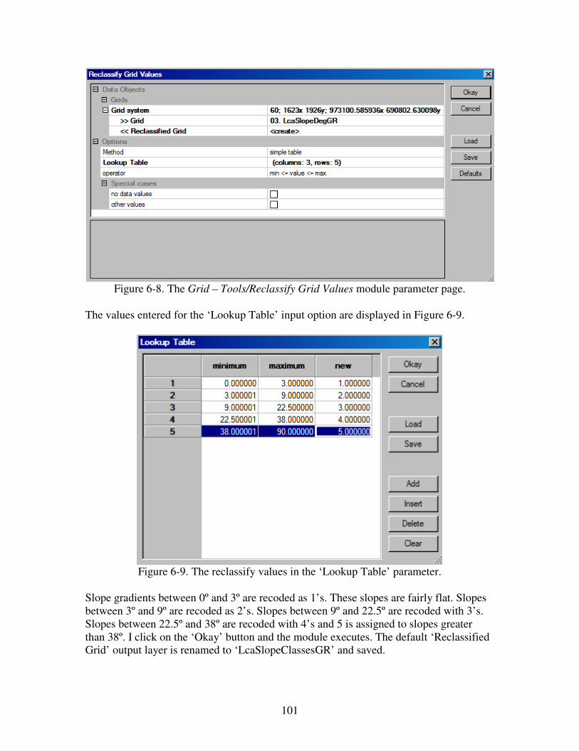
101
Figure 6-8. The Grid – Tools/Reclassify Grid Values module parameter page.
The values entered for the ‘Lookup Table’ input option are displayed in Figure 6-9.
Figure 6-9. The reclassify values in the ‘Lookup Table’ parameter.
Slope gradients between 0º and 3º are recoded as 1’s. These slopes are fairly flat. Slopes
between 3º and 9º are recoded as 2’s. Slopes between 9º and 22.5º are recoded with 3’s.
Slopes between 22.5º and 38º are recoded with 4’s and 5 is assigned to slopes greater
than 38º. I click on the ‘Okay’ button and the module executes. The default ‘Reclassified
Grid’ output layer is renamed to ‘LcaSlopeClassesGR’ and saved.

102
I use the Spatial and Geostatistics – Grids/Zonal Grid Statistics module to count the
number of cells from each aspect and slope class on the ‘LcaAspectClassesGR’ and
‘LcaSlopeClassesGR’ grid data layers for each of the least cost path corridor grid data
layers. Figure 6-10 displays the parameter page for the Spatial and Geostatistics –
Grids/Zonal Grid Statistics module with the ‘LcaAspectClassesGR’ layer for the
‘>>Zone Grid’ parameter.
Figure 6-10. The parameter page for the Spatial and Geostatistics – Grids/Zonal Grid
Statistics module.
The parameters displayed in Figure 6-10 will generate aspect class cell counts for each of
the five least cost path corridor layers chosen for the ‘>Grids to analyse’ parameter. The
“[create]” option is entered for the output parameter ‘<<Zonal Statistics’. I click on the
‘Okay’ button and the module executes.
The default output is a table named ‘Zonal Statistics’. I deleted statistical fields from this
table that I did not need. Figure 6-11 displays the cell count fields in the ‘Zonal Statistics’
table. Numbers of cells in the aspect classes for each of the five least cost path solutions
are listed in this table.
Figure 6-11. Sample ‘Zonal Statistics’ tabular output.
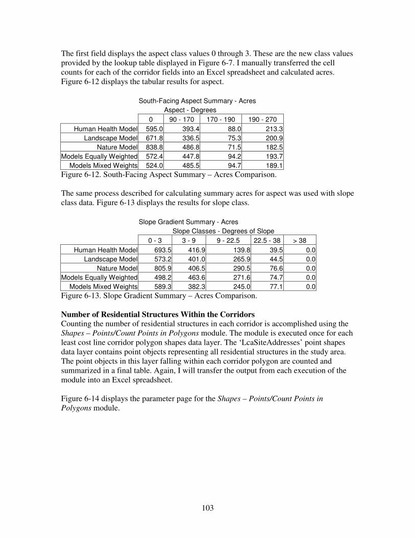
103
The first field displays the aspect class values 0 through 3. These are the new class values
provided by the lookup table displayed in Figure 6-7. I manually transferred the cell
counts for each of the corridor fields into an Excel spreadsheet and calculated acres.
Figure 6-12 displays the tabular results for aspect.
South-Facing Aspect Summary - Acres
Aspect - Degrees
0 90 - 170 170 - 190 190 - 270
Human Health Model 595.0 393.4 88.0 213.3
Landscape Model 671.8 336.5 75.3 200.9
Nature Model 838.8 486.8 71.5 182.5
Models Equally Weighted 572.4 447.8 94.2 193.7
Models Mixed Weights 524.0 485.5 94.7 189.1
Figure 6-12. South-Facing Aspect Summary – Acres Comparison.
The same process described for calculating summary acres for aspect was used with slope
class data. Figure 6-13 displays the results for slope class.
Slope Gradient Summary - Acres
Slope Classes - Degrees of Slope
0 - 3 3 - 9 9 - 22.5 22.5 - 38 > 38
Human Health Model 693.5 416.9 139.8 39.5 0.0
Landscape Model 573.2 401.0 265.9 44.5 0.0
Nature Model 805.9 406.5 290.5 76.6 0.0
Models Equally Weighted 498.2 463.6 271.6 74.7 0.0
Models Mixed Weights 589.3 382.3 245.0 77.1 0.0
Figure 6-13. Slope Gradient Summary – Acres Comparison.
Number of Residential Structures Within the Corridors
Counting the number of residential structures in each corridor is accomplished using the
Shapes – Points/Count Points in Polygons module. The module is executed once for each
least cost line corridor polygon shapes data layer. The ‘LcaSiteAddresses’ point shapes
data layer contains point objects representing all residential structures in the study area.
The point objects in this layer falling within each corridor polygon are counted and
summarized in a final table. Again, I will transfer the output from each execution of the
module into an Excel spreadsheet.
Figure 6-14 displays the parameter page for the Shapes – Points/Count Points in
Polygons module.
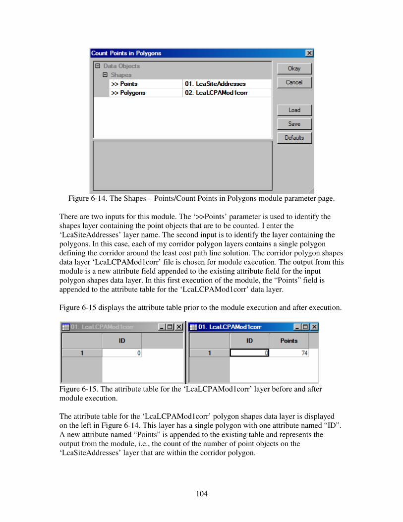
104
Figure 6-14. The Shapes – Points/Count Points in Polygons module parameter page.
There are two inputs for this module. The ‘>>Points’ parameter is used to identify the
shapes layer containing the point objects that are to be counted. I enter the
‘LcaSiteAddresses’ layer name. The second input is to identify the layer containing the
polygons. In this case, each of my corridor polygon layers contains a single polygon
defining the corridor around the least cost path line solution. The corridor polygon shapes
data layer ‘LcaLCPAMod1corr’ file is chosen for module execution. The output from this
module is a new attribute field appended to the existing attribute field for the input
polygon shapes data layer. In this first execution of the module, the “Points” field is
appended to the attribute table for the ‘LcaLCPAMod1corr’ data layer.
Figure 6-15 displays the attribute table prior to the module execution and after execution.
Figure 6-15. The attribute table for the ‘LcaLCPAMod1corr’ layer before and after
module execution.
The attribute table for the ‘LcaLCPAMod1corr’ polygon shapes data layer is displayed
on the left in Figure 6-14. This layer has a single polygon with one attribute named “ID”.
A new attribute named “Points” is appended to the existing table and represents the
output from the module, i.e., the count of the number of point objects on the
‘LcaSiteAddresses’ layer that are within the corridor polygon.

105
I execute the Shapes – Points/Count Points in Polygons module once for each corridor
polygon shapes data layer. Figure 6-16 displays the summary table developed in Excel.
# of
Residences
Human Health Model 74
Landscape Model 154
Nature Model 483
Models Equally Weighted 179
Models Mixed Weights 120
Figure 6-16. The number of residences within each corridor.
Comparing Estimated Market Value of ROW Property
The purpose of this criterion is to get an impression of the relative market value of
corridor property for each model.
A polygon shapes data layer named ‘LcaParcelsVAL’ exists for the study area. This layer
was derived from the Mason County layer for land parcel values. The attribute table for
this layer includes an attribute for the square foot size of each parcel (“SHAPE_AREA”)
and another identifying the market value (“MARKET_VAL”) for each parcel. I will use
these attributes to calculate a new attribute for the acre size of each parcel and the parcel
per acre market value.
Before using the Table – Calculus/Table Calculator (Shapes) module to calculate acres
and market value numbers, I have to create two new attribute fields in the attribute table
for the ‘LcaParcelsVAL’ layer. I name the first one “ACRES” and place it in the table
immediately following the existing “SHAPE_AREA” attribute. It is important, as you
will see, to keep track of the field number for this new attribute. It becomes field number
17. Next I create a new attribute named “PERACRVAL” and place it after the new
“ACRES” field. It becomes field number 18. Both of these new fields are defined as “8
byte floating point number” storage types. Where I place these new fields relative to the
other fields does not make any difference.
These two fields are easily added to the attribute table. First, I click on the name of the
polygon shapes data layer (‘LcaParcelsVAL’) in the ‘Data’ tab area of the Workspace.
When I click the right mouse button the pop-up list of options displays one toward the
bottom named “Attributes”. I move the mouse cursor down over the “Attributes” name
and another menu appears. I choose the “Show” option and the attribute table is displayed
in the work area.
In the display of the attribute table, I move the mouse pointer into the table row
displaying the attribute (field) names. I press the right mouse button and a pop-up list of
options appears. I choose the “Add Field” option. The ‘Add Field’ dialog window
displays (Figure 6-17).
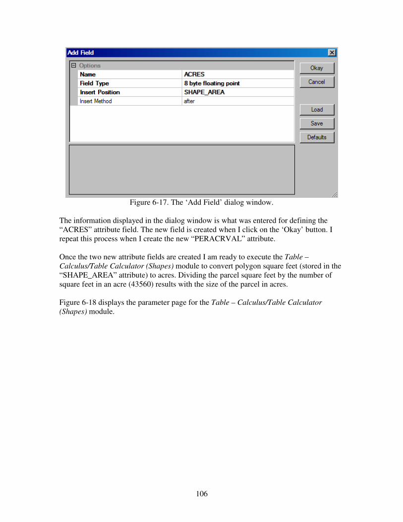
106
Figure 6-17. The ‘Add Field’ dialog window.
The information displayed in the dialog window is what was entered for defining the
“ACRES” attribute field. The new field is created when I click on the ‘Okay’ button. I
repeat this process when I create the new “PERACRVAL” attribute.
Once the two new attribute fields are created I am ready to execute the Table –
Calculus/Table Calculator (Shapes) module to convert polygon square feet (stored in the
“SHAPE_AREA” attribute) to acres. Dividing the parcel square feet by the number of
square feet in an acre (43560) results with the size of the parcel in acres.
Figure 6-18 displays the parameter page for the Table – Calculus/Table Calculator
(Shapes) module.
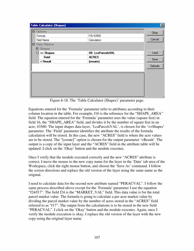
107
Figure 6-18. The ‘Table Calculator (Shapes)’ parameter page.
Equations entered for the ‘Formula’ parameter refer to attributes according to their
column location in the table. For example, f16 is the reference for the “SHAPE_AREA”
field. The equation entered for the ‘Formula’ parameter uses the value (square feet) in
field 16, the “SHAPE_AREA” field, and divides it by the number of square feet in an
acre, 43560. The input shapes data layer, ‘LcaParcelsVAL’, is chosen for the ‘>>Shapes’
parameter. The ‘Field’ parameter identifies the attribute the results of the formula
calculation will be stored. In this case, the new “ACRES” field is where the acre values
are to be stored. The “[create]” option is chosen for the output parameter ‘<Result’. The
output is a copy of the input layer and the “ACRES” field in the attribute table will be
updated. I click on the ‘Okay’ button and the module executes.
Once I verify that the module executed correctly and the new “ACRES” attribute is
correct, I move the mouse to the new copy name for the layer in the ‘Data’ tab area of the
Workspace, click the right mouse button, and choose the ‘Save As’ command. I follow
the screen directions and replace the old version of the layer using the same name as the
original.
I need to calculate data for the second new attribute named “PERACVAL”. I follow the
same process described above except for the ‘Formula’ parameter I use the equation
“f24/f17”. The field f24 is the “MARKET_VAL” field. This data value is for the total
parcel market value. The formula is going to calculate a per acre market value by
dividing the parcel market value by the number of acres stored in the “ACRES” field
referred to as “f17”. The output from the calculations is to be stored in the new field
“PERACVAL”. I click on the ‘Okay’ button and the module executes. Again, once I
verify the module execution is okay, I replace the old version of the layer with the new
copy using the original layer name.
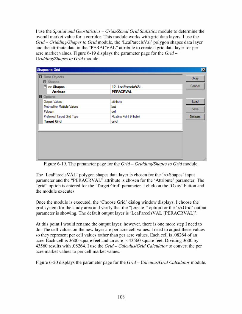
108
I use the Spatial and Geostatistics – Grids/Zonal Grid Statistics module to determine the
overall market value for a corridor. This module works with grid data layers. I use the
Grid – Gridding/Shapes to Grid module, the ‘LcaParcelsVal’ polygon shapes data layer
and the attribute data in the “PERACVAL” attribute to create a grid data layer for per
acre market values. Figure 6-19 displays the parameter page for the Grid –
Gridding/Shapes to Grid module.
Figure 6-19. The parameter page for the Grid – Gridding/Shapes to Grid module.
The ‘LcaParcelsVAL’ polygon shapes data layer is chosen for the ‘>>Shapes’ input
parameter and the “PERACRVAL” attribute is chosen for the ‘Attribute’ parameter. The
“grid” option is entered for the ‘Target Grid’ parameter. I click on the ‘Okay’ button and
the module executes.
Once the module is executed, the ‘Choose Grid’ dialog window displays. I choose the
grid system for the study area and verify that the “[create]” option for the ‘<<Grid’ output
parameter is showing. The default output layer is ‘LcaParcelsVAL [PERACRVAL]’.
At this point I would rename the output layer, however, there is one more step I need to
do. The cell values on the new layer are per acre cell values. I need to adjust these values
so they represent per cell values rather than per acre values. Each cell is .08264 of an
acre. Each cell is 3600 square feet and an acre is 43560 square feet. Dividing 3600 by
43560 results with .08264. I use the Grid – Calculus/Grid Calculator to convert the per
acre market values to per cell market values.
Figure 6-20 displays the parameter page for the Grid – Calculus/Grid Calculator module.

109
Figure 6-20. The Grid – Calculus/Grid Calculator module parameter page.
The default output grid data layer from the Shapes to Grid module is entered for the
‘>>Grids’ parameter, ‘LcaParcelsVAL [PERACRVAL]’. The equation entered for the
‘Formula’ parameter is “a*.08264” where “a” is the variable representing the input grid
data layer. The output grid data layer is named ‘LcaValPerCellGR’. I save it.
The Spatial and Geostatistics – Grids/Zonal Grid Statistics module parameter page is
displayed in Figure 6-21.
Figure 6-21. The Spatial and Geostatistics – Grids/Zonal Grid Statistics module
parameter page.

110
The line solution corridor is used for two inputs in this module. First, it is chosen as the
‘>>Zone Grid’ parameter. The objective is for the market values for grid cells within the
corridor to be totaled. The grid data layer containing per cell market values,
‘LcaValPerCellGR’, is one of the two grid data layers chosen for the ‘>Grids to analyse’
parameter. The second grid data layer is the ‘LcaLCPAMod1corrGR’ layer. The
“[create]” option is chosen for the ‘<<Zonal Statistics’ output parameter. The default
table output is named ‘Zonal Statistics’.
The ‘Zonal Statistics’ output table is displayed in Figure 6-22.
Figure 6-22. The ‘Zonal Statistics’ output table for the Human Health model line solution
corridor.
The second row of the table contains statistics for the ‘LcaLCPAMod1corrGR’ grid data
layer including the sum for all the data values coinciding with the corridor for the
‘LcaValPerCellGR’ layer. The total market value for the corridor is in the second row,
the last field. It is listed at 27013686.845820.
I execute the Spatial and Geostatistics – Grids/Zonal Grid Statistics module once for
each least cost line solution corridor. The estimated corridor market values are displayed
in the table below.
Estimated Corridor Land Market Value
Human Health Model $27,013,687
Landscape Model $41,993,535
Nature Model $125,081,656
Models Equally Weighted $39,610,429
Models Mixed Weights $36,046,155
Figure 6-23. Estimated Corridor Market Value
Comparing Land Use Class Differences
The last evaluation criterion is comparing acres of land use differences between the
corridors. I use the Spatial and Geostatistics – Grids/Zonal Grid Statistics module with
the area land use layer, ‘LcaGenLUGR’. The parameter page for the Spatial and
Geostatistics – Grids/Zonal Grid Statistics module is displayed in Figure 6-24.
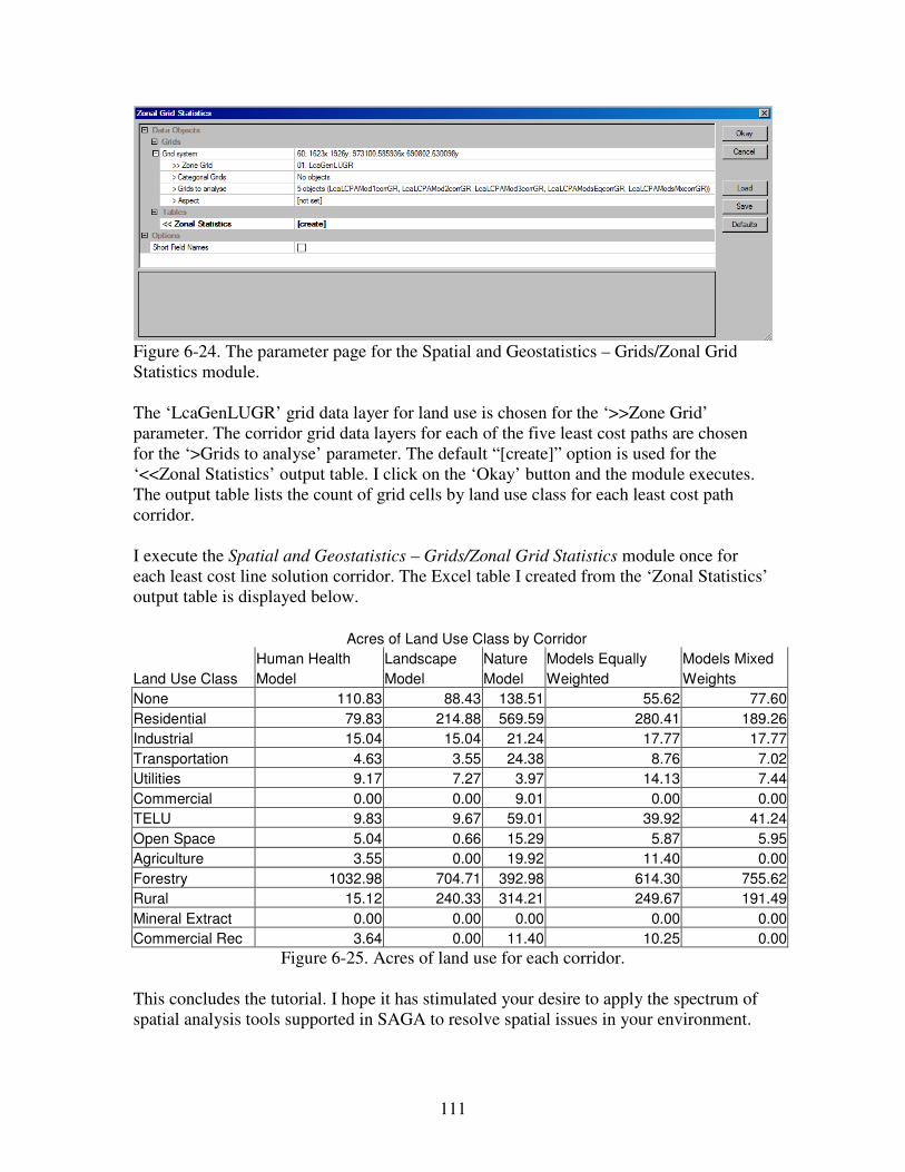
111
Figure 6-24. The parameter page for the Spatial and Geostatistics – Grids/Zonal Grid
Statistics module.
The ‘LcaGenLUGR’ grid data layer for land use is chosen for the ‘>>Zone Grid’
parameter. The corridor grid data layers for each of the five least cost paths are chosen
for the ‘>Grids to analyse’ parameter. The default “[create]” option is used for the
‘<<Zonal Statistics’ output table. I click on the ‘Okay’ button and the module executes.
The output table lists the count of grid cells by land use class for each least cost path
corridor.
I execute the Spatial and Geostatistics – Grids/Zonal Grid Statistics module once for
each least cost line solution corridor. The Excel table I created from the ‘Zonal Statistics’
output table is displayed below.
Acres of Land Use Class by Corridor
Human Health Landscape Nature Models Equally Models Mixed
Land Use Class Model Model Model Weighted Weights
None 110.83 88.43 138.51 55.62 77.60
Residential 79.83 214.88 569.59 280.41 189.26
Industrial 15.04 15.04 21.24 17.77 17.77
Transportation 4.63 3.55 24.38 8.76 7.02
Utilities 9.17 7.27 3.97 14.13 7.44
Commercial 0.00 0.00 9.01 0.00 0.00
TELU 9.83 9.67 59.01 39.92 41.24
Open Space 5.04 0.66 15.29 5.87 5.95
Agriculture 3.55 0.00 19.92 11.40 0.00
Forestry 1032.98 704.71 392.98 614.30 755.62
Rural 15.12 240.33 314.21 249.67 191.49
Mineral Extract 0.00 0.00 0.00 0.00 0.00
Commercial Rec 3.64 0.00 11.40 10.25 0.00
Figure 6-25. Acres of land use for each corridor.
This concludes the tutorial. I hope it has stimulated your desire to apply the spectrum of
spatial analysis tools supported in SAGA to resolve spatial issues in your environment.

112
There are many opportunities to implement “What if” scenarios once the models are
developed and the output understood.
For example, the there are two levels of importance weights. Weights are applied at both
the factor element and model levels. I did develop output for two sets of weights at the
model level. The factor element weights can also be adjusted and the cost surface layers
recreated. Weight changes can be developed that support a wide range of perspectives.
The Grid – Calculus/Fuzzify module could be used in place of the Grid – Calculus/Grid
Normalisation module for rescaling data ranges. In particular, the rescaling of distances
could be used to reduce the spatial area of influence. In this tutorial, I used the full range
of distance values produced by the Grid – Tools/Proximity Grid module. Using Fuzzify
the rescale could include a cutoff distance of one mile. This would reduce the effect of
distance but increase the importance within a smaller area.
There are many opportunities for adjustments.

113
References
The reference below authored by Bagli et al provided a starting point for the hypothetical
structure of this tutorial.
Bagli, Stefano, Davide Geneletti, and Francesco Orsi. “Routeing of power lines through
least-cost path analysis and multicriteria evaluation to minimize environmental impacts.”
Environmental Impact Assessment Review 31 (2011): pp. 234-239.
Other References Used
Anavberokhai, Isah O. “Introducing GIS and Multi-Criteria Analysis in Road Path
Planning Process in Nigeria.” M.Sc. Thesis, University of Gavle, Department of
Technology and Built Environment, 2008, 37 pages.
Choi, Y.S., H. D. Park, C. Sunwoo. “Multi-Criteria Evaluation and Least Cost Path
Analysis for Optimal Haulage Routing in Open-Pit Mines. Web published report.
Collischonn, Walter and Jorge Victor Pilar. “A Direction Dependent Least Cost Path
Algorithm for Roads and Canals”. International Journal of Geographical Information
Systems 14(4): 397-406 (2000).
Delavar, Mahmoud Reza and Fereydoon Naghibi. “Pipeline Routing Using Geospatial
Information System Analysis.” ScanGIS’ 2003 Conference Proceedings, June 4-6, 2003.
Pages 203-213.
Landscapes Limited. PERMITS Methodology (Process of Energy Routing to Minimize
Impact from Transmission Systems). Madison, Wisconsin: 1972.
LaRue, Michelle and Clayton K. Nielsen. “Modelling Potential Dispersal Corridors for
Cougars in Midwestern North America Using Least-Cost Path Methods.” Ecological
Modelling 212: 372-381 (2008).
Lloyd, Christopher. Spatial Data Analysis: An Introduction for GIS Users, New York,
Oxford University Press, 2010, pp. 162-170.
Menke, Kurt. Locating Potential Cougar (Puma concolor) Corridors in New Mexico
Using a Least-Cost Path Corridor GIS Analysis. Wildlife Final Project Report Contract
#08-516-0000-00005, May 31, 2008, 40 pages.
Saha, A. K., M. K. Arora, R. P. Gupta, M. L. Virdi, and E. Csaplovics. “GIS-Based
Route Planning in Landslide-Prone Areas.” International Journal of Geographic
Information Systems 19 (10): 1149-1175 (2005).
Stahl, Christopher. “Accumulated Surfaces & Least-Cost Paths: GIS Modeling for
Autonomous Ground Vehicles (AGV) Navigation”. M.Sc. Thesis, Virginia Polygtechnic
Institute and State University, 2005, 94 pages.

114
Yu, Chaoqing, Jay Lee and Mandy J. Munro-Stasiuk. “Extensions to Least-Cost Path
Algorithms for Roadway Planning.” International Journal of Geographical Information
Systems 17 (4): 361-376 (2003).

115
Appendix A
This appendix lists the dataset files used in this tutorial. Some notes are included related
to how the layer was created and processed. File names in bold are included in the data
folder. These, generally, are input files for SAGA modules. The rest of the files are
output files from SAGA modules and are not included in the data folder.
County_Parks. Mason County GIS point shapes data layer with point objects
representing county park locations.
LcaAccumHthModGR. Grid data layer created by the Accumulated Cost (Isotropic)
module. Input layers are LcaCostHthModGR and LcaDestinationPointGR. Grid cell data
values from the LcaCostHthModGR layer are accumulated in cells radiating from the
single destination cell on the LcaDestinationPointGR grid data layer.
LcaAccumLandModGR. Grid data layer created by the Accumulated Cost (Isotropic)
module. Input layers are LcaCostLandModGR and LcaDestinationPointGR. Grid cell
data values from the LcaCostLandModGR layer are accumulated in cells radiating from
the single destination cell on the LcaDestinationPointGR grid data layer.
LcaAccumNatrModGR. Grid data layer created by the Accumulated Cost (Isotropic)
module. Input layers are LcaCostNatrModGR and LcaDestinationPointGR. Grid cell data
values from the LcaCostNatrModGR layer are accumulated in cells radiating from the
single destination cell on the LcaDestinationPointGR grid data layer.
LcaAccumAllModsEqGR. Grid data layer created by the Accumulated Cost (Isotropic)
module. Input layers are LcaCostAllModsEqGR and LcaDestinationPointGR. Grid cell
data values from the LcaCostAllModsEqGR layer are accumulated in cells radiating from
the single destination cell on the LcaDestinationPointGR grid data layer.
LcaAccumAllModsMxGR. Grid data layer created by the Accumulated Cost (Isotropic)
module. Input layers are LcaCostAllModsMxGR and LcaDestinationPointGR. Grid cell
data values from the LcaCostAllModsMxGR layer are accumulated in cells radiating
from the single destination cell on the LcaDestinationPointGR grid data layer.
LcaAddressDistGR. A grid data layer where grid cells contain distances the cells are
from address features to no data cells. The Proximity Grid module created this output
layer. The Grid Masking module was used to convert data values outside of the study
area boundary to no data values –99999.
LcaAddressDistGRNM. A grid data layer produced by the Grid Normalisation module.
The data range of the LcaAddressDistGR layer is rescaled to a range of continuous data
values from 0 to 1.
LcaAspectClassesGR. Grid data layer. Grid – Tools/Reclassify Grid Values module
recoded aspect values on LcaAspectDegGR into 4 discrete aspect classes.

116
LcaAspectDegGR. A grid data layer created by the Terrain Analysis –
Morphometry/Slope, Aspect, Curvature module from an input digital elevation module.
Output values were originally in radians. The values were converted to degrees using the
Grid – Calculus/Grid Calculator module to multiply each radian cell value by
57.2957795.
LcaAspectDegGRFUZ. A grid data layer. The input layer for the Grid – Calculus/Fuzzify
module is the LcaAspectDegGR layer. Aspect values from 0º to 90º were set to 0; from
90º to 170º rescaled increasing from 0 to 1; from 170º to 190º set to 1; from 190º to 270º
rescaled decreasing from 1 to 0; and from 270º to 360º set to 0.
LcaBuffWidthGR. A grid data layer created with the Grid – Tools/Proximity Grid
module. Grid data values are distances grid cells are to no data cells from ridges.
LcaCommParks. A point shapes data layer derived by selecting 4 community park point
objects on the LcaSiteAddresses layer. The Shapes-Tools/Copy Selection to New Shapes
Layer module was used to create a new layer for the four selected point objects.
LcaCostHthModGR. A grid data layer representing surface cost for the human health
model. Produced by the Grid Calculator module by applying importance weights to cell
values on the LcaAddressDistGRNM, LcaPopEstimateGRNM, and
LcaSchoolsDistGRNM layers and adding the corresponding cells for output to the
corresponding cell of the output layer.
LcaCostLandModGR. A grid data layer representing surface cost for the landscape
model. Produced by the Grid Calculator module by applying importance weights to the
cell values on the LcaParksLibsDistGRNM, LcaVisibleAllGRNM,
LcaSensBldgDistGRNM and LcaVisibldgAllGRNM layers and adding the
corresponding cells for output to the corresponding cell of the output layer.
LcaCostNatrModGR. A grid data layer representing surface cost for the nature model.
Produced by the Grid Calculator module by applying importance weights to the cell
values on the LcaAspectDegGRFUZ, LcaStrtBuffDistGRNM, LcaGenLUGRRE and
LcaRidgeBuffRecDistGRNM layers and adding the corresponding cells for output to the
corresponding cell of the output layer.
LcaCostAllModsEqGR. A grid data layer representing surface cost for the composite of
the three models. Produced by the Grid Calculator module by applying equal model
importance weights to the cell values on the LcaCostHthModGR, LcaCostLandModGR,
and LcaCostNatrModGR layers and adding the corresponding cells for output to the
corresponding cell of the output layer.
LcaCostAllModsMxGR. A grid data layer representing surface cost for the composite of
the three models. Produced by the Grid Calculator module by applying varying model
importance weights to the cell values on the LcaCostHthModGR, LcaCostLandModGR,
117
and LcaCostNatrModGR layers and adding the corresponding cells for output to the
corresponding cell of the output layer.
LcaCountyParks. Point shapes data layer. Point objects represent county park locations
in the study area. Derived from Mason County GIS County_Parks point shapes data
layer.
LcaDEMfeetGR. Grid data layer for digital elevation model for the study area.
Elevations are in feet.
LcaDestinationPointGR. A grid data layer. One cell within the study area identifies the
northern substation. All other cells contain no data values. The Grid – Gridding/Shapes
to Grid module produced the module using the input point shapes data layer
LcaDestinationPoint.
LcaDestinationPoint. A point shapes data layer. A single point within the study area
identifies the northern substation.
LcaGenLUGR. A grid data layer. The general land use layer for the study area. There
are 12 land use classes.
LcaGenLUGRRE. A grid data layer. The Grid – Tools/Reclassify Grid Values module
was used to reclassify the data values on the LcaGenLUGR layer to cost impact values
between 0 and 1.
LcaLandformsGR. A grid data layer. This layer was produced by the Terrain Analysis –
Morphometry/TPI Based Landform Classification module and has 10 discrete landform
classes. The DEM layer ‘LcaDEMfeetGR’ was the input layer for the module.
LcaLCPAMod1corr. Polygon shapes data layer. This layer contains a single polygon
object delineating a 300’ buffer on both sides of the line (as the corridor) for the
LcaLCPALineMod1 line shapes data layer. The Shapes – Tools/Shapes Buffer module
created the corridor layer.
LcaLCPAMod2corr. Polygon shapes data layer. This layer contains a single polygon
object delineating a 300’ buffer on both sides of the line (as the corridor) for the
LcaLCPALineMod2 line shapes data layer. The Shapes – Tools/Shapes Buffer module
created the corridor layer.
LcaLCPAMod3corr. Polygon shapes data layer. This layer contains a single polygon
object delineating a 300’ buffer on both sides of the line (as the corridor) for the
LcaLCPALineMod3 line shapes data layer. The Shapes – Tools/Shapes Buffer module
created the corridor layer.
LcaLCPAModEqcorr. Polygon shapes data layer. This layer contains a single polygon
object delineating a 300’ buffer on both sides of the line (as the corridor) for the
118
LcaLCPALineModEq line shapes data layer. The Shapes – Tools/Shapes Buffer module
created the corridor layer.
LcaLCPAModMxcorr. Polygon shapes data layer. This layer contains a single polygon
object delineating a 300’ buffer on both sides of the line (as the corridor) for the
LcaLCPALineModMx line shapes data layer. The Shapes – Tools/Shapes Buffer module
created the corridor layer.
LcaLCPAMod1corrGR. Grid data layer. This is a raster conversion of the
LcaLCPAMod1corr polygon shapes data layer. The Grid – Gridding/Shapes to Grid was
used for the conversion.
LcaLCPAMod2corrGR. Grid data layer. This is a raster conversion of the
LcaLCPAMod2corr polygon shapes data layer. The Grid – Gridding/Shapes to Grid was
used for the conversion.
LcaLCPAMod3corrGR. Grid data layer. This is a raster conversion of the
LcaLCPAMod3corr polygon shapes data layer. The Grid – Gridding/Shapes to Grid was
used for the conversion.
LcaLCPAModEqcorrGR. Grid data layer. This is a raster conversion of the
LcaLCPAModEqcorr polygon shapes data layer. The Grid – Gridding/Shapes to Grid
was used for the conversion.
LcaLCPAModMxcorrGR. Grid data layer. This is a raster conversion of the
LcaLCPAModMxcorr polygon shapes data layer. The Grid – Gridding/Shapes to Grid
was used for the conversion.
LcaLCPALineMod1. Line shapes data layer produced by the Grid – Analysis/Least Cost
Paths module. Input to the module is the LcaAccumHthModGR accumulated cost grid
data layer and the LcaSourcePoint point shapes data layer. The location of the line is the
least cost path between the destination and source points.
LcaLCPAPointsMod1. Point shapes data layer produced by the Grid – Analysis/Least
Cost Paths module. Input to the module is the LcaAccumHthModGR accumulated cost
grid data layer and the LcaSourcePoint point shapes data layer. The point objects on the
output are the grid cells the least cost path traverses between the destination and source
points.
LcaLCPALineMod2. Line shapes data layer produced by the Grid – Analysis/Least Cost
Paths module. Input to the module is the LcaAccumLandModGR accumulated cost grid
data layer and the LcaSourcePoint point shapes data layer. The location of the line is the
least cost path between the destination and source points.
LcaLCPAPointsMod2. Point shapes data layer produced by the Grid – Analysis/Least
Cost Paths module. Input to the module is the LcaAccumLandModGR accumulated cost

119
grid data layer and the LcaSourcePoint point shapes data layer. The point objects on the
output are the grid cells the least cost path traverses between the destination and source
points.
LcaLCPALineMod3. Line shapes data layer produced by the Grid – Analysis/Least Cost
Paths module. Input to the module is the LcaAccumNatrModGR accumulated cost grid
data layer and the LcaSourcePoint point shapes data layer. The location of the line is the
least cost path between the destination and source points.
LcaLCPAPointsMod3. Point shapes data layer produced by the Grid – Analysis/Least
Cost Paths module. Input to the module is the LcaAccumNatrModGR accumulated cost
grid data layer and the LcaSourcePoint point shapes data layer. The point objects on the
output are the grid cells the least cost path traverses between the destination and source
points.
LcaLCPALineModsEq. Line shapes data layer produced by the Grid – Analysis/Least
Cost Paths module. Input to the module is the LcaAccumAllModsEqGR accumulated
cost grid data layer and the LcaSourcePoint point shapes data layer. The location of the
line is the least cost path between the destination and source points.
LcaLCPAPointsModsEq. Point shapes data layer produced by the Grid – Analysis/Least
Cost Paths module. Input to the module is the LcaAccumAllModsEqGR accumulated
cost grid data layer and the LcaSourcePoint point shapes data layer. The point objects on
the output are the grid cells the least cost path traverses between the destination and
source points.
LcaLCPALineModsMx. Line shapes data layer produced by the Grid – Analysis/Least
Cost Paths module. Input to the module is the LcaAccumAllModsMxGR accumulated
cost grid data layer and the LcaSourcePoint point shapes data layer. The location of the
line is the least cost path between the destination and source points.
LcaLCPAPointsModsMx. Point shapes data layer produced by the Grid – Analysis/Least
Cost Paths module. Input to the module is the LcaAccumAllModsMxGR accumulated
cost grid data layer and the LcaSourcePoint point shapes data layer. The point objects on
the output are the grid cells the least cost path traverses between the destination and
source points.
LcaLibraries. A point shapes data layer derived from the Mason County GIS point
shapes layer (Libraries) of library locations. Point objects represent public libraries in the
study area.
LcaNon-CountyParks. Point shapes data layer. Point objects represent non-county park
locations in the study area. Derived from Mason County GIS Non-County_Parks point
shapes data layers.

120
LcaParcelsVAL. Polygon shapes data layer. Parcel polygons for study area from Mason
County GIS Parcels layer. Two attributes added supporting calculation of corridor market
values.
LcaParksLibs. Point shapes data layer. Point objects represent county parks, non-county
parks, and public libraries in study area. LcaCountyParks, LcaNon-CountyParks,
LcaCommParks, and LcaLibraries point shapes data layers were merged together using
the Shapes-Tools/Merge Shapes Layers module.
LcaParksLibsDistGR. A grid data layer created by the Proximity Grid module. Distance
values are calculated from county, non-county, and community parks and library
locations on the grid data layer LcaParksLibsGR to no data values on the layer.
LcaParksLibsDistGRNM. A grid data layer created by the Grid Normalisation module.
The data range on the input LcaParksLibsDistGR layer was rescaled to the continuous dta
value range 0 to 1.
LcaParksLibsGR. Grid data layer version of point shapes data layer LcaParksLibs.
Created using Grid – Gridding/Shapes to Grid module.
LcaPopEstimateGR. A grid data layer created originally by the Grid – Gridding/Kernel
Density Estimation module. The LcaSiteAddresses point shapes data layer is input. The
Grid – Tools/Reclassify Grid Values module applied for recoding. The Grid – Tools/Grid
Masking module used to convert data values outside of the study area to no data value –
99999.
LcaPopEstimateGRNM. A grid data layer produced by the Grid Normalisation module.
The LcaPopEstimateGR layer was the input layer. The data range is rescaled to a range of
continuous data values from 0 to 1.
LcaPopEstTEMPGR. A grid data layer. This layer is the saved version of the default
output from the Grid – Gridding/Kernel Density Estimation module after the no data
value of 0 is changed to –99999 using the layer setting “No Data”.
LcaRidgeBuffersTEMP. A grid data layer. The default ‘Buffer’ layer output by the Grid
– Tools/Threshold Buffer module.
LcaRidgeBuffRecGR. A grid data layer. The Grid – Tools/Reclassify Grid Values
module was used to recode 1’s and 2’s on the LcaRidgeBuffersTEMP layer and to
change the no data value –2147483647 to –99999. The Grid – Tools/Grid Masking
module was used to convert data values outside of the study area to no data values –
99999. The Masked Grid default output layer was named LcaRidgeBuffRecGR.
LcaRidgeBuffRecDistGR. A grid data layer. The LcaRidgeBuffRecGR layer was input to
the Proximity Grid module. Data values represent cell distances from cells containing a
121
ridge buffers to no data cells. The Grid – Tools/Grid Masking module was used to
convert distance values outside of the study area to no data values –99999.
LcaRidgeBuffRecDistGRNM. A grid data layer. Distance values on the
LcaRidgeBuffRecDistGR layer are rescaled to the continuous data value range 0 to 1
using the Grid – Tools/Grid Normalisation module.
LcaRidgesBuffCritGR. A grid data layer created by the Grid – Calculus/Grid Calculator
module. Input layers are LcaRidgesGR containing “1”s for ridges and the DEM layer for
the study area LcaDEMfeetGR. The data values on this layer define the criteria for buffer
width around ridge grid cells.
LcaRidgesGR. A grid data layer. The Grid – Calculus/Grid Calculator module was used
to select the “high ridges” discrete data category on the LcaLandformsGR layer. A new,
temporary layer was output. The Grid – Tools/Grid Masking layer was used to convert
data values outside of the study area to no data values (-99999). The output layer Masked
Grid was renamed LcaRidgesGR.
LcaSchools. A point shapes data layer. Point objects represent the location of schools
within the study area. This layer was derived from the Mason County GIS Schools point
shapes data layer.
LcaSchoolsDistGR. A grid data layer created by the Proximity Grid module. Data values
represent cell distances from cells containing a school to no data cells. The Grid Masking
module was used to recode distance data values outside of the study area to no data
values –99999.
LcaSchoolsDistGRNM. A grid data layer produced by the Grid Normalisation module.
The data range on the LcaSchoolsDistGR is rescaled to a range of continuous data values
from 0 to 1.
LcaSchoolsGR. A grid data layer created with the Grid – Gridding/Shapes to Grid
module. Input was the point shapes data layer LcaSchools.
LcaSensBldg. A point shapes data layer. Point objects represent “sensitive” non-
residential buildings in the study area. There are 43 point objects.
LcaSensBldgGR. A grid data layer. A grid data layer version of shapes layer
LcaSensBldg. Created using Grid – Gridding/Shapes to Grid module.
LcaSensBldgDistGR. A grid data layer produced by the Proximity Grid module. Data
values represent cell distances from cells containing a sensitive building to no data value
cells on the LcaSensBldgGR grid data layer.

122
LcaSensBldgDistGRNM. A grid data layer. This layer was created using the Grid –
Calculus/Grid Normalisation module. The original data range on the
LcaSensBldgDistGR layer was rescaled to continuous data values in the range of 0 to 1.
LcaSiteAddresses. A point shapes data layer derived from the Mason County site
address layer (Site_Address).
LcaSiteAddressesGR. A grid data layer version of the point shapes data layer
LcaSiteAddresses. The layer was created by the Shapes to Grid module.
LcaSlopeDegGR. Grid data layer. Continuous slope gradient values for the study area.
Slope calculated with Terrain Analysis – Morphometry/Slope, Aspect, Curvature module
and LcaDEMfeetGR layer of elevation values as input.
LcaSlopeClassesGR. Grid data layer. Grid – Tools/Reclassify Grid Values module
recoded slope values on LcaSlopeDegGR into 5 discrete slope classes.
LcaSourcePoint. A point shapes data layer. A single point within the study area
identifies the southern substation.
LcaStreetCentBuff. A polygon shapes data layer. This layer was created using the Shapes
– Tools/Shapes Buffer module. The layer contains one polygon object made up of
multiple “parts”. The polygon is a buffer or corridor around federal, state, county, and
Forest Service roads. The corridor width varies by type; 1500’ for federal roads, 900’ for
state, 600’ for county, and 300’ for Forest Service.
LcaStreetCentBuffGR. A grid data layer. This is the grid version of the polygon shapes
data layer LcaStreetCentBuff. The Grid – Gridding/Shapes to Grid module created this
layer.
LcaStreetCentBuffDistGR. A grid data layer. This layer was created by the Grid –
Tools/Proximity Grid module using the LcaStreetCentBuffGR layer as input. Cell values
represent the distance the cell is from the “features”, i.e., corridors, on the input layer to
no data grid cells.
LcaStrtBuffDistGRNM. A grid data layer. The Grid Normalisation module was used to
rescale the data range on the LcaStreetCentBuffDistGR layer to continuous data values
from the 0 to 1 range.
LcaStreetCenterlines. A line shapes data layer. This layer contains road locations in the
study area. It was derived from the Mason County GIS Street_Centerlines line shapes
data layer. The “CORWIDTH” attribute in the linked attribute table contains corridor
width data for federal, state, county, and US Forest Service roads.
LcaStudyArea. A polygon shapes data layer containing one polygon delineating the
study area boundary.

123
LcaStudyAreaGR. A grid data layer. The grid system is rectangular in shape; the study
area has a partially irregular shape within the rectangle. The study area grid cells have 1’s
and grid cells outside of the study area have no data values –99999. This layer was
produced from the LcaStudyArea polygon shapes data layer using the Shapes to Grid
module. Used often with the Grid – Tools/Grid Masking module.
LcaVisibleAllGRNM. A grid data layer. The Grid Normalisation module was used to
rescale the data range on the VisibleAllGR layer to values ranging from 0 to 1.
LcaVisibldgAllGRNM. A grid data layer. The Grid Normalisation module was used to
rescale the data range on the VisibldgAllGR layer to values ranging from 0 to 1.
Libraries. Mason County GIS point shapes data layer with point objects representing
public libraries.
Non-County_Parks. Mason County GIS point shapes data layer with point objects
representing non-county parks.
Parcels. Mason County GIS polygon shapes data layer.
Schools. Mason County GIS point shapes data layer with point objects representing
schools.
Site_Address. Point shapes data layer. The Mason County GIS site address layer.
Street_Centerlines. Line shapes data layer. The Mason County GIS street centerline
layer.
Visible01 through Visible40. Grid data layers representing foreground and middleground
viewshed from park and library sites. Original grid data layer is the default Visible layer
output by the interactive module Terrain Analysis – Lighting, Visibility/Visibility (single
point) [interactive]. No data values –99999 were recoded to 0’s using the Grid –
Tools/Reclassify Grid Values module. The Visiblenn layer was produced by the Grid
Calculator module that changed distance values greater than 3 miles to 0’s and distance
values greater than 0 but less than 3 miles to 1’s. Data values are 1’s and 0’s.
Visibldg01 through Visibldg43. Grid data layers representing foreground and
middleground viewshed from sensitive building sites. Original grid data layer is the
default Visible layer output by the interactive module Terrain Analysis – Lighting,
Visibility/Visibility (single point) [interactive]. No data values –99999 were recoded to
0’s using the Grid – Tools/Reclassify Grid Values module. The Visiblenn layer was
produced by the Grid Calculator module that changed distance values greater than 3
miles to 0’s and distance values greater than 0 but less than 3 miles to 1’s. Data values
are 1’s and 0’s.
124
VisibldgAllGR. Grid data layer created using Grid Calculator module. Added Visibldg01
through Visibldg43 together. No data values –99999 were recoded to 0’s using the Grid –
Tools/Reclassify Grid Values module. Data range is from 1 to 13.
VisibldgAllTEMPGR. Grid data layer created using Grid Calculator module. An interim
layer used as input for the Grid Masking module.
VisibleAllGR. Grid data layer created using Grid Calculator module. Visible01 through
Visible40 grid data layers are added together. No data values –99999 were recoded to 0’s
using the Grid – Tools/Reclassify Grid Values module. Data range is from 1 to 12.
VisibleAllTEMPGR. Grid data layer created using Grid Calculator module. An interim
layer used as input for the Grid Masking module.


![The saga of Saga Hill [by] Theodore C. Blegen.](https://static.fdocuments.us/doc/165x107/61a59bc0e6a2046cbe681bd9/the-saga-of-saga-hill-by-theodore-c-blegen.jpg)