Sample to Insight

Tutorial

De Novo Assembly of Paired DataNovember 21, 2017

QIAGEN Aarhus Silkeborgvej 2 Prismet 8000 Aarhus C DenmarkTelephone: +45 70 22 32 44 www.qiagenbioinformatics.comAdvancedGenomicsSupport@qiagen.com

Tutorial

De Novo Assembly of Paired Data 2

De Novo Assembly of Paired DataA de novo assembly involves taking many short sequences and trying to assemble them intolonger, contiguous sequences. We recommend that you read about how the de novo assemblytool works before running this tool on your own data. You can read more in our manual http://resources.qiagenbioinformatics.com/manuals/clcgenomicsworkbench/current/index.php?manual=De_novo_sequencing.html or in the White Paper: http://resources.qiagenbioinformatics.com//white-papers/White_paper_on_de_novo_assembly_4.pdf.

This tutorial takes you through a typical de novo sequencing work flow with paired sequence data.We will

• Search and import sequence read data.

• Run a quality check on the read data.

• Trim the reads based on quality.

• Run a de novo assembly, including scaffolding.

We also include optional sections on finding broken pair mates in mapping results and exportingcontigs from a set of mappings.

Import the data into the Workbench We will use two Illumina read sets from Pseudomonasaeruginosa, one mate-pair data, and the other paired-end data. The data is available from theShort Read Archive under the Study Accession SRP010152.

To download the data:

1. In the workbench go to Download | Search for Reads in SRA.

2. Enter the study accession number and click Start search.

3. Select SRR396636 and SRR396637. Click Download Reads and Metadata (figure 1).

Figure 1: Importing mate-pair and paired-end Illumina data.

4. You can select "Discard read names" to save some time and space on your machine butkeep "Discard quality scores" unchecked. Click Next.

5. In the parameters dialog, the workbench gives some distance estimates. You can seethat there is a difference between the two data sets, due to the fact that SRR396636

Tutorial

De Novo Assembly of Paired Data 3

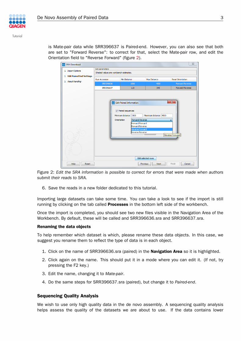
is Mate-pair data while SRR396637 is Paired-end. However, you can also see that bothare set to "Forward Reverse": to correct for that, select the Mate-pair row, and edit theOrientation field to "Reverse Forward" (figure 2).

Figure 2: Edit the SRA information is possible to correct for errors that were made when authorssubmit their reads to SRA.

6. Save the reads in a new folder dedicated to this tutorial.

Importing large datasets can take some time. You can take a look to see if the import is stillrunning by clicking on the tab called Processes in the bottom left side of the workbench.

Once the import is completed, you should see two new files visible in the Navigation Area of theWorkbench. By default, these will be called and SRR396636.sra and SRR396637.sra.

Renaming the data objects

To help remember which dataset is which, please rename these data objects. In this case, wesuggest you rename them to reflect the type of data is in each object.

1. Click on the name of SRR396636.sra (paired) in the Navigation Area so it is highlighted.

2. Click again on the name. This should put it in a mode where you can edit it. (If not, trypressing the F2 key.)

3. Edit the name, changing it to Mate-pair.

4. Do the same steps for SRR396637.sra (paired), but change it to Paired-end.

Sequencing Quality Analysis

We wish to use only high quality data in the de novo assembly. A sequencing quality analysishelps assess the quality of the datasets we are about to use. If the data contains lower

Tutorial

De Novo Assembly of Paired Data 4

quality regions, it should be trimmed, and the trimmed sequences used as input to the de novoassembly. If there are over-represented sequence motifs in the data, then it is worth checking ifany adapters remain. If so, it is very important that these be trimmed away before using the datafor de novo assembly.

Running a quality analysis

Here, we run the Create Sequencing QC Report tool on both our sequence data objects. We willuse the batch functionality, allowing us to simultaneously launch the analysis of multiple sets ofdata.

1. Go to:

Toolbox | NGS Core Tools ( ) | Create Sequencing QC Report

2. Check the box labeled Batch at the bottom of the Wizard window. Note that if the boxlabeled Batch is not checked, you will only be able to move data objects to the SelectedElements pane on the right, not folders, and you will generate only one report instead ofone report per element.

3. Click on the folder containing your sequence data objects and then click the arrow pointingright. This will move the folder into the right hand pane as shown in figure 3. Click Next.

Figure 3: Set up a batch job for running a quality check analysis.

4. The next window allows you to fine tune which data objects the analysis should run on. Ifyou click on either of the object names in the left hand side, the data object(s) to be workedon will be listed on the right hand side. Here, each folder contains only the data that wewish to work with, so we can just proceed to the next step.

5. Check the boxes labeled Create graphical report and Create supplementary report.Uncheck the box labeled Create duplicated sequence list. Check the box labeled Save ininput folder to save the results before clicking on the button labeled Finish.

When both the quality check analyses are finished, you should see graphical and summaryreports for each of your data sets listed in the Navigation Area.

Investigating the Sequencing Quality Check Reports

Here, we wish to look at the quality distribution for the reads and the sequence duplicationinformation.

1. Open the file called Mate-pair - graphical QC report and take a look at the content.

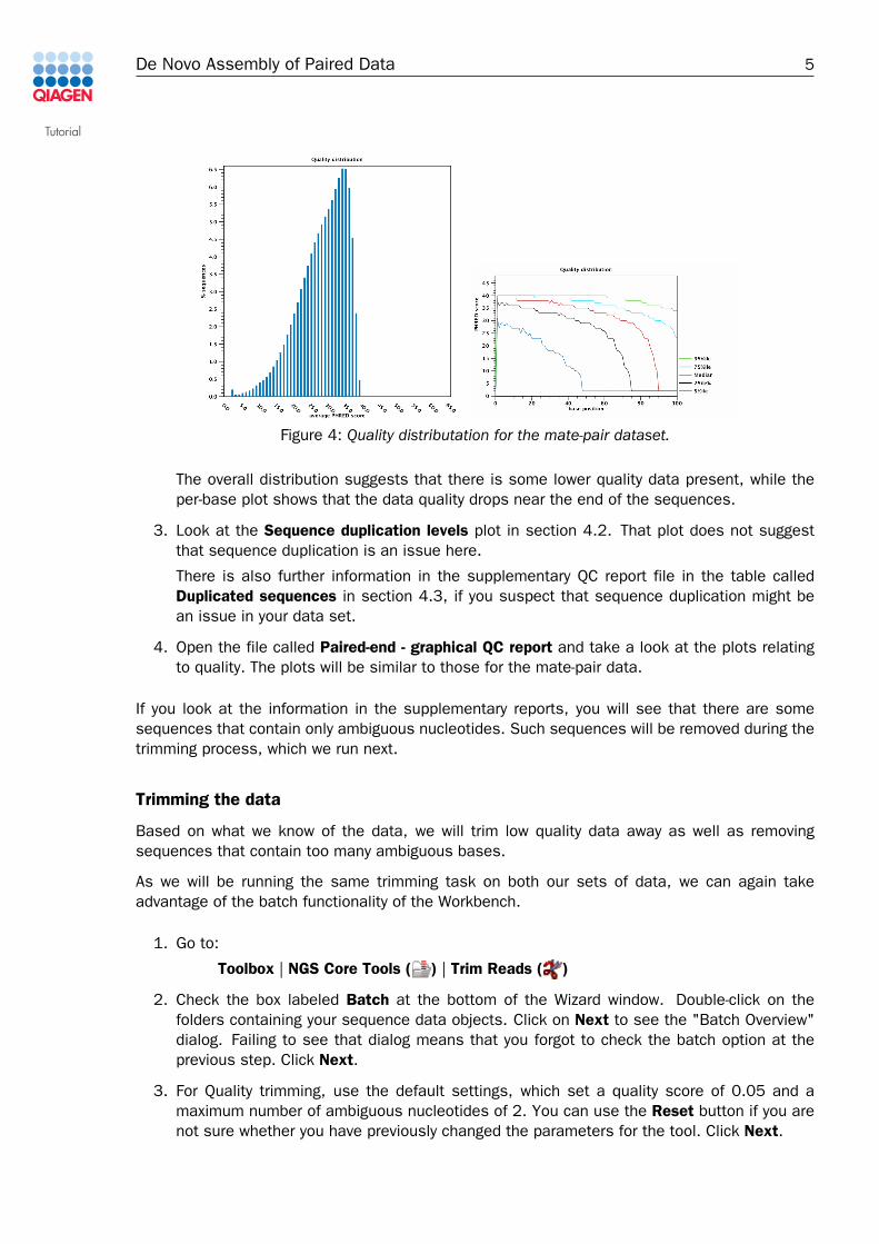
2. Look at the Quality distribution plots in section 2.4 and 3.5 as shown in figure 4.

Tutorial

De Novo Assembly of Paired Data 5

Figure 4: Quality distributation for the mate-pair dataset.

The overall distribution suggests that there is some lower quality data present, while theper-base plot shows that the data quality drops near the end of the sequences.

3. Look at the Sequence duplication levels plot in section 4.2. That plot does not suggestthat sequence duplication is an issue here.

There is also further information in the supplementary QC report file in the table calledDuplicated sequences in section 4.3, if you suspect that sequence duplication might bean issue in your data set.

4. Open the file called Paired-end - graphical QC report and take a look at the plots relatingto quality. The plots will be similar to those for the mate-pair data.

If you look at the information in the supplementary reports, you will see that there are somesequences that contain only ambiguous nucleotides. Such sequences will be removed during thetrimming process, which we run next.

Trimming the data

Based on what we know of the data, we will trim low quality data away as well as removingsequences that contain too many ambiguous bases.

As we will be running the same trimming task on both our sets of data, we can again takeadvantage of the batch functionality of the Workbench.

1. Go to:

Toolbox | NGS Core Tools ( ) | Trim Reads ( )

2. Check the box labeled Batch at the bottom of the Wizard window. Double-click on thefolders containing your sequence data objects. Click on Next to see the "Batch Overview"dialog. Failing to see that dialog means that you forgot to check the batch option at theprevious step. Click Next.

3. For Quality trimming, use the default settings, which set a quality score of 0.05 and amaximum number of ambiguous nucleotides of 2. You can use the Reset button if you arenot sure whether you have previously changed the parameters for the tool. Click Next.

Tutorial

De Novo Assembly of Paired Data 6

4. Adapter trimming will be performed as set by default, i.e., with the "Automatic read-throughadapter trimming" option checked. Make sure there is no Trim adapter list specified in theAdapter trimming section of the wizard. If you had run an adapter trimming previously, andan trim adapter list appears in this wizard step, please use the Reset button to clear theprevious settings and click Next.

5. For Sequence filtering, check the option "Discard reads below length" and set the number15. Click Next.

6. In the Output options section, choose to Save broken pairs and to Create report. Save theresults in the input folder and click on the button labeled Finished.

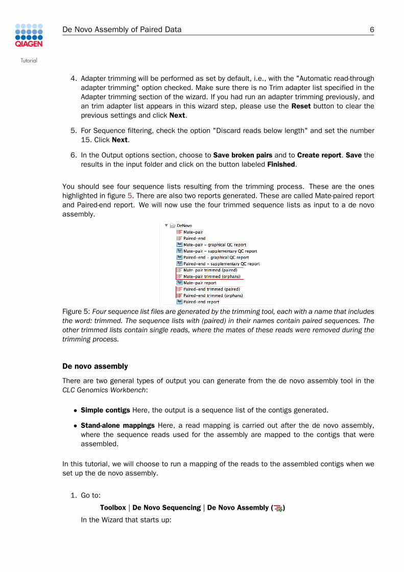
You should see four sequence lists resulting from the trimming process. These are the oneshighlighted in figure 5. There are also two reports generated. These are called Mate-paired reportand Paired-end report. We will now use the four trimmed sequence lists as input to a de novoassembly.

Figure 5: Four sequence list files are generated by the trimming tool, each with a name that includesthe word: trimmed. The sequence lists with (paired) in their names contain paired sequences. Theother trimmed lists contain single reads, where the mates of these reads were removed during thetrimming process.

De novo assembly

There are two general types of output you can generate from the de novo assembly tool in theCLC Genomics Workbench:

• Simple contigs Here, the output is a sequence list of the contigs generated.

• Stand-alone mappings Here, a read mapping is carried out after the de novo assembly,where the sequence reads used for the assembly are mapped to the contigs that wereassembled.

In this tutorial, we will choose to run a mapping of the reads to the assembled contigs when weset up the de novo assembly.

1. Go to:

Toolbox | De Novo Sequencing | De Novo Assembly ( )

In the Wizard that starts up:

Tutorial

De Novo Assembly of Paired Data 7

2. Select the four sequence lists that were generated by the trimming tool: Mate-pairtrimmed (paired), Mate-pair trimmed (orphans), Paired-end trimmed (paired) and Paired-end trimmed (orphans). Click Next.

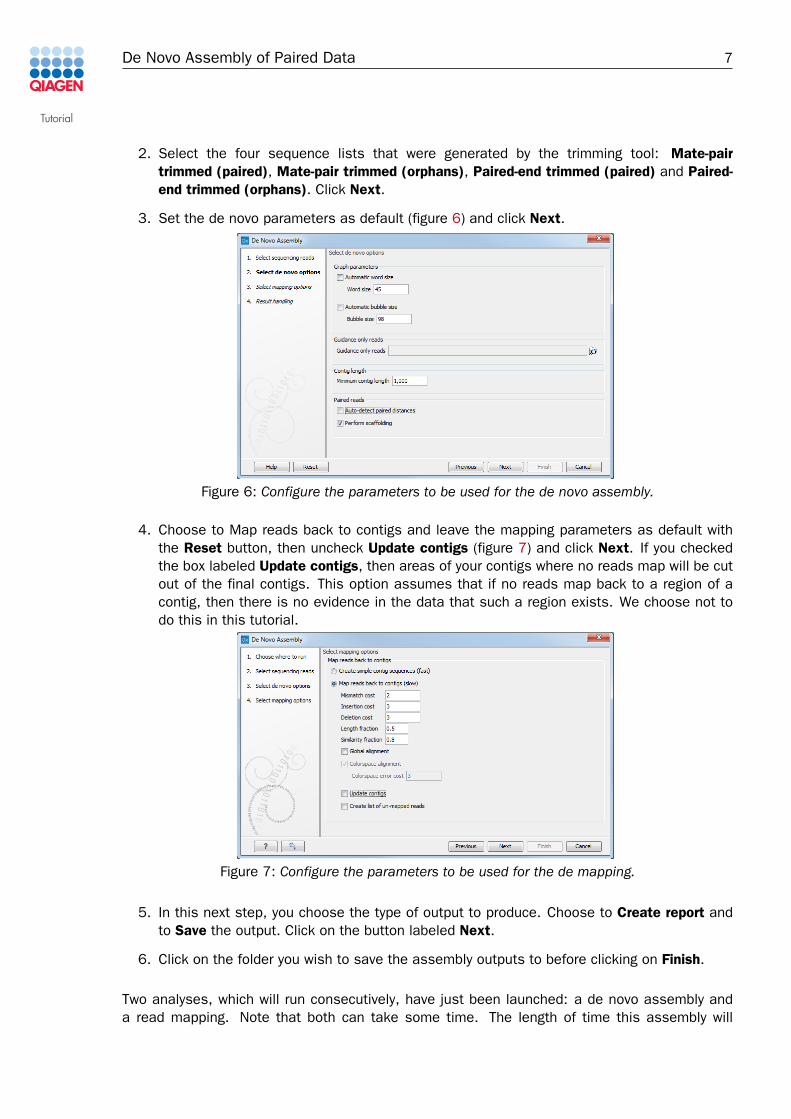
3. Set the de novo parameters as default (figure 6) and click Next.

Figure 6: Configure the parameters to be used for the de novo assembly.

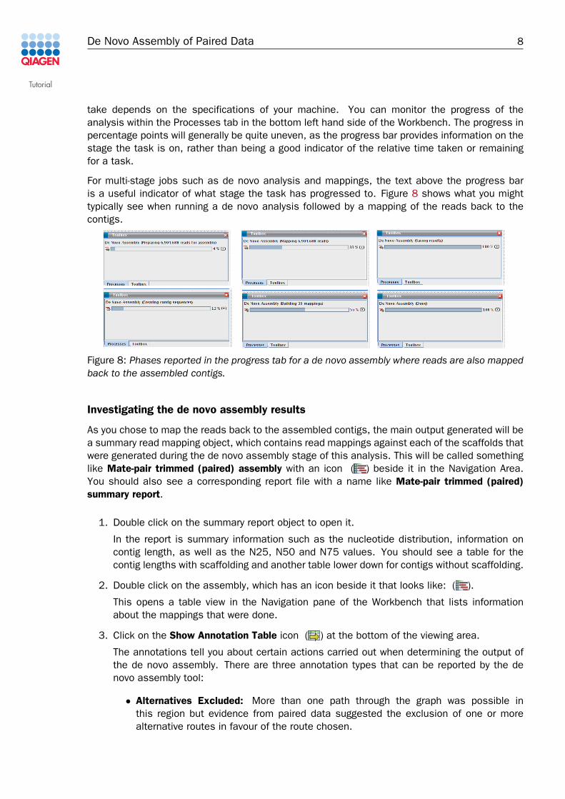
4. Choose to Map reads back to contigs and leave the mapping parameters as default withthe Reset button, then uncheck Update contigs (figure 7) and click Next. If you checkedthe box labeled Update contigs, then areas of your contigs where no reads map will be cutout of the final contigs. This option assumes that if no reads map back to a region of acontig, then there is no evidence in the data that such a region exists. We choose not todo this in this tutorial.

Figure 7: Configure the parameters to be used for the de mapping.

5. In this next step, you choose the type of output to produce. Choose to Create report andto Save the output. Click on the button labeled Next.

6. Click on the folder you wish to save the assembly outputs to before clicking on Finish.

Two analyses, which will run consecutively, have just been launched: a de novo assembly anda read mapping. Note that both can take some time. The length of time this assembly will

Tutorial

De Novo Assembly of Paired Data 8

take depends on the specifications of your machine. You can monitor the progress of theanalysis within the Processes tab in the bottom left hand side of the Workbench. The progress inpercentage points will generally be quite uneven, as the progress bar provides information on thestage the task is on, rather than being a good indicator of the relative time taken or remainingfor a task.

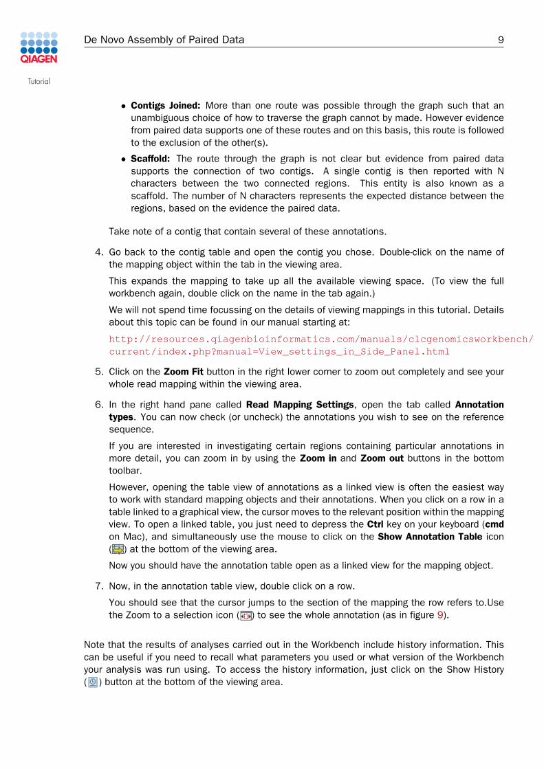
For multi-stage jobs such as de novo analysis and mappings, the text above the progress baris a useful indicator of what stage the task has progressed to. Figure 8 shows what you mighttypically see when running a de novo analysis followed by a mapping of the reads back to thecontigs.

Figure 8: Phases reported in the progress tab for a de novo assembly where reads are also mappedback to the assembled contigs.

Investigating the de novo assembly results

As you chose to map the reads back to the assembled contigs, the main output generated will bea summary read mapping object, which contains read mappings against each of the scaffolds thatwere generated during the de novo assembly stage of this analysis. This will be called somethinglike Mate-pair trimmed (paired) assembly with an icon ( ) beside it in the Navigation Area.You should also see a corresponding report file with a name like Mate-pair trimmed (paired)summary report.

1. Double click on the summary report object to open it.

In the report is summary information such as the nucleotide distribution, information oncontig length, as well as the N25, N50 and N75 values. You should see a table for thecontig lengths with scaffolding and another table lower down for contigs without scaffolding.

2. Double click on the assembly, which has an icon beside it that looks like: ( ).

This opens a table view in the Navigation pane of the Workbench that lists informationabout the mappings that were done.

3. Click on the Show Annotation Table icon ( ) at the bottom of the viewing area.

The annotations tell you about certain actions carried out when determining the output ofthe de novo assembly. There are three annotation types that can be reported by the denovo assembly tool:

• Alternatives Excluded: More than one path through the graph was possible inthis region but evidence from paired data suggested the exclusion of one or morealternative routes in favour of the route chosen.

Tutorial

De Novo Assembly of Paired Data 9

• Contigs Joined: More than one route was possible through the graph such that anunambiguous choice of how to traverse the graph cannot by made. However evidencefrom paired data supports one of these routes and on this basis, this route is followedto the exclusion of the other(s).

• Scaffold: The route through the graph is not clear but evidence from paired datasupports the connection of two contigs. A single contig is then reported with Ncharacters between the two connected regions. This entity is also known as ascaffold. The number of N characters represents the expected distance between theregions, based on the evidence the paired data.

Take note of a contig that contain several of these annotations.

4. Go back to the contig table and open the contig you chose. Double-click on the name ofthe mapping object within the tab in the viewing area.

This expands the mapping to take up all the available viewing space. (To view the fullworkbench again, double click on the name in the tab again.)

We will not spend time focussing on the details of viewing mappings in this tutorial. Detailsabout this topic can be found in our manual starting at:

http://resources.qiagenbioinformatics.com/manuals/clcgenomicsworkbench/current/index.php?manual=View_settings_in_Side_Panel.html

5. Click on the Zoom Fit button in the right lower corner to zoom out completely and see yourwhole read mapping within the viewing area.

6. In the right hand pane called Read Mapping Settings, open the tab called Annotationtypes. You can now check (or uncheck) the annotations you wish to see on the referencesequence.

If you are interested in investigating certain regions containing particular annotations inmore detail, you can zoom in by using the Zoom in and Zoom out buttons in the bottomtoolbar.

However, opening the table view of annotations as a linked view is often the easiest wayto work with standard mapping objects and their annotations. When you click on a row in atable linked to a graphical view, the cursor moves to the relevant position within the mappingview. To open a linked table, you just need to depress the Ctrl key on your keyboard (cmdon Mac), and simultaneously use the mouse to click on the Show Annotation Table icon( ) at the bottom of the viewing area.

Now you should have the annotation table open as a linked view for the mapping object.

7. Now, in the annotation table view, double click on a row.

You should see that the cursor jumps to the section of the mapping the row refers to.Usethe Zoom to a selection icon ( ) to see the whole annotation (as in figure 9).

Note that the results of analyses carried out in the Workbench include history information. Thiscan be useful if you need to recall what parameters you used or what version of the Workbenchyour analysis was run using. To access the history information, just click on the Show History( ) button at the bottom of the viewing area.

Tutorial

De Novo Assembly of Paired Data 10

Figure 9: Double clicking on the row shown highlighted in the table above jumps the cursor to thepoint in the mapping view shown below. If you wish to, you can change the colors of the annotationsdisplayed by just clicking in the coloured box next to each annotation type, and selecting a newcolor.

Finding broken pair mates

Reads mapped back to the contigs where both partners of a pair map in the correct relativeorientation and within the expected distance range are coloured blue in the mapping and arecalled an intact pair. Those where only one member of the pair mapped, or those where bothpartners mapped, but in the wrong relative orientation or outside the expected distance range areconsidered members of a broken pair. Members of a broken pair that map to a unique locationagainst the reference are colored green or red, according to whether they mapped in the forwardor reverse orientation respectively.

To investigate where mapped mates of a broken pair are in the assembly:

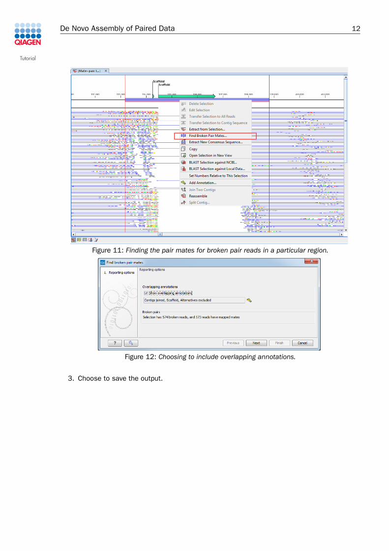
1. Highlight a region of interest. For example, find a scaffold annotation where you see greenand red coloured lines on either side of the gap, and highlight the region around this, asshown in figure 11.

2. Right click the mouse cursor over the highlighted region (underneath the annotation).Choose the option Find Broken Pair Mates as shown in figure 11.

3. Check the Show overlapping annotations box and select all annotation types present afterclicking on the yellow arrow icon in the wizard (figure 12). Note that a summary of thenumber of broken pairs in the region selected is also given in this dialog. Click Next.

4. Choose to Open the results and click on the button labeled Finish.

Tutorial

De Novo Assembly of Paired Data 11

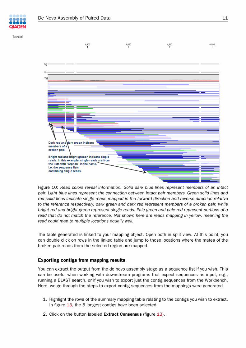
Figure 10: Read colors reveal information. Solid dark blue lines represent members of an intactpair. Light blue lines represent the connection between intact pair members. Green solid lines andred solid lines indicate single reads mapped in the forward direction and reverse direction relativeto the reference respectively; dark green and dark red represent members of a broken pair, whilebright red and bright green represent single reads. Pale green and pale red represent portions of aread that do not match the reference. Not shown here are reads mapping in yellow, meaning theread could map to multiple locations equally well.

The table generated is linked to your mapping object. Open both in split view. At this point, youcan double click on rows in the linked table and jump to those locations where the mates of thebroken pair reads from the selected region are mapped.

Exporting contigs from mapping results

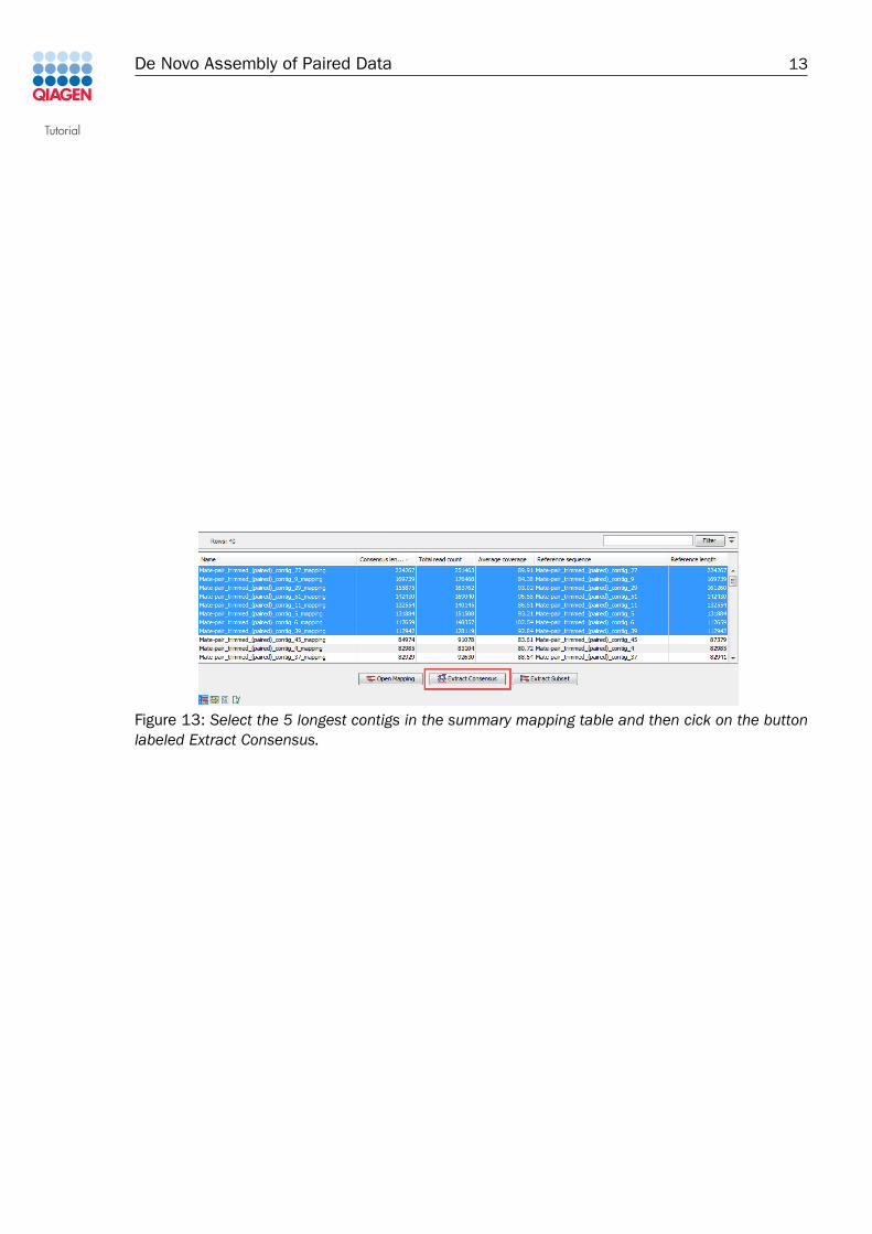
You can extract the output from the de novo assembly stage as a sequence list if you wish. Thiscan be useful when working with downstream programs that expect sequences as input, e.g.,running a BLAST search, or if you wish to export just the contig sequences from the Workbench.Here, we go through the steps to export contig sequences from the mappings were generated.

1. Highlight the rows of the summary mapping table relating to the contigs you wish to extract.In figure 13, the 5 longest contigs have been selected.

2. Click on the button labeled Extract Consensus (figure 13).

Tutorial

De Novo Assembly of Paired Data 12

Figure 11: Finding the pair mates for broken pair reads in a particular region.

Figure 12: Choosing to include overlapping annotations.

3. Choose to save the output.

Tutorial

De Novo Assembly of Paired Data 13

Figure 13: Select the 5 longest contigs in the summary mapping table and then cick on the buttonlabeled Extract Consensus.