Tutorial on Optimal Control Theory: Application to the LQ...
55
Tutorial on Optimal Control Theory: Application to the LQ problem Séminaire COPHY 27 mars 2014 Marc JUNGERS
Transcript of Tutorial on Optimal Control Theory: Application to the LQ...
Tutorial on Optimal ControlTheory: Application to the LQ
problem
Séminaire COPHY27 mars 2014
Marc JUNGERS

Issue of the presentation
Provide some elements to cope with optimization problems in theframework of optimal control theory :• Euler-Lagrange equations• Pontryaguin Maximum Principle (necessary conditions of optimality)• Dynamic Programming (sufficient conditions of optimality)
How these tools may be applied to the Linear Quadratic problem ?
Introduction 2 / 55 M. Jungers
Outline of the talk
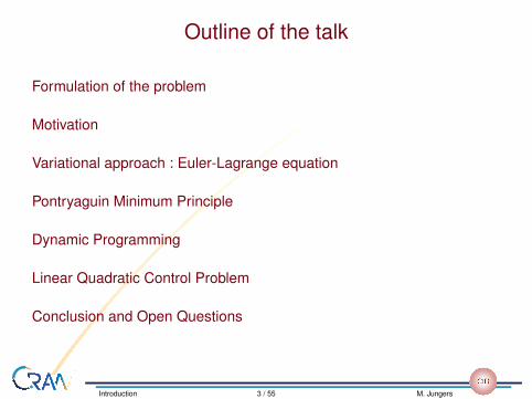
Formulation of the problem
Motivation
Variational approach : Euler-Lagrange equation
Pontryaguin Minimum Principle
Dynamic Programming
Linear Quadratic Control Problem
Conclusion and Open Questions
Introduction 3 / 55 M. Jungers
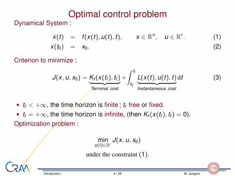
Optimal control problemDynamical System :
x(t) = f (x(t),u(t), t), x ∈ Rn, u ∈ Rr . (1)x(t0) = x0. (2)
Criterion to minimize :
J(x ,u, x0) = Kf (x(tf ), tf )︸ ︷︷ ︸Terminal cost
+
∫ tf
t0L(x(t),u(t), t)︸ ︷︷ ︸Instantaneous cost
dt (3)
• tf < +∞, the time horizon is finite ; tf free or fixed.• tf = +∞, the time horizon is infinite, (then Kf (x(tf ), tf ) = 0).
Optimization problem :
minu(t)∈Rr
J(x ,u, x0)
under the constraint (1).
Introduction 4 / 55 M. Jungers
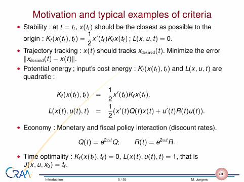
Motivation and typical examples of criteria• Stability : at t = tf , x(tf ) should be the closest as possible to the
origin : Kf (x(tf ), tf ) =12
x ′(tf )Kf x(tf ) ; L(x ,u, t) = 0.
• Trajectory tracking : x(t) should tracks xdesired(t). Minimize the error‖xdesired(t)− x(t)‖.
• Potential energy ; input’s cost energy : Kf (x(tf ), tf ) and L(x ,u, t) arequadratic :
Kf (x(tf ), tf ) =12
x ′(tf )Kf x(tf );
L(x(t),u(t), t) =12
(x ′(t)Q(t)x(t) + u′(t)R(t)u(t)).
• Economy : Monetary and fiscal policy interaction (discount rates).
Q(t) = e2αtQ; R(t) = e2αtR.
• Time optimality : Kf (x(tf ), tf ) = 0, L(x(t),u(t), t) = 1, that isJ(x ,u, x0) = tf .
Introduction 5 / 55 M. Jungers

Formulation of the problem
Motivation
Variational approach : Euler-Lagrange equation
Pontryaguin Minimum Principle
Dynamic Programming
Linear Quadratic Control Problem
Conclusion and Open Questions
Introduction 6 / 55 M. Jungers
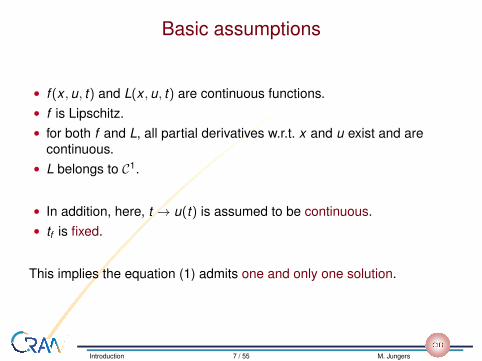
Basic assumptions
• f (x ,u, t) and L(x ,u, t) are continuous functions.• f is Lipschitz.• for both f and L, all partial derivatives w.r.t. x and u exist and are
continuous.• L belongs to C1.
• In addition, here, t → u(t) is assumed to be continuous.• tf is fixed.
This implies the equation (1) admits one and only one solution.
Introduction 7 / 55 M. Jungers
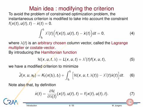
Main idea : modifying the criterionTo avoid the problem of constrained optimization problem, theinstantaneous criterion is modified to take into account the constraintf (x(t),u(t), t)− x(t) = 0.
∫ tf
t0λ′(t)
(f (x(t),u(t), t)− x(t)
)dt = 0, (4)
where λ(t) is an arbitrary chosen column vector, called the Lagrangemultiplier or costate-vector.By introducing the Hamiltonian function
H(x ,u, t , λ) = L(x ,u, t) + λ′(t)f (x ,u, t), (5)
we have a modified criterion to minimize
J(x ,u, x0) = Kf (x(tf ), tf ) +
∫ tf
t0
[H(x ,u, t , λ(t))− λ′(t)x(t)
]dt . (6)
Note also that, by definition
x(t) =∂H∂λ(t)
(x(t),u(t), t) = f (x(t),u(t), t). (7)
Introduction 8 / 55 M. Jungers

Refomulation of the criterion
By using the integration by parts
−∫ tf
t0)
λ′(t)x(t)dt = −λ′(tf )x(tf ) + λ′(t0)x0 +
∫ tf
t0λ′(t)x(t)dt , (8)
one gets
J =
∫ tf
t0
[H(x ,u, t , λ(t))+λ′(t)x(t)
]dt+
[Kf (x(tf ), tf )−λ′(tf )x(tf )
]+λ′(t0)x0.
(9)
Introduction 9 / 55 M. Jungers

First order necessary conditions (I)
By assuming that u∗(t) is a continuous optimal control input, solution ofthe optimization problem. The associated trajectory is denoted x∗(t).
Considering
u(t) = u∗(t) + δu(t); (10)
x(t) = x∗(t) + δx(t) (11)
x!(t)
x!(t) + !x(t)
!x(tf )
!x(t0)
1
leads to the inequality
J(x∗,u∗, x0) ≤ J(x∗ + δx ,u∗ + δu, x0), ∀δx , δu. (12)
The first order necessary condition consists in the fact that J(x∗,u∗, x0)is an extremum.
Introduction 10 / 55 M. Jungers
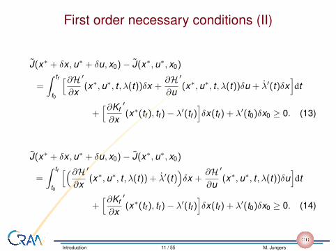
First order necessary conditions (II)
J(x∗ + δx ,u∗ + δu, x0)− J(x∗,u∗, x0)
=
∫ tf
t0
[∂H∂x
′(x∗,u∗, t , λ(t))δx +
∂H∂u
′(x∗,u∗, t , λ(t))δu + λ′(t)δx
]dt
+[∂Kf
∂x
′(x∗(tf ), tf )− λ′(tf )
]δx(tf ) + λ′(t0)δx0 ≥ 0. (13)
J(x∗ + δx ,u∗ + δu, x0)− J(x∗,u∗, x0)
=
∫ tf
t0
[(∂H∂x
′(x∗,u∗, t , λ(t)) + λ′(t)
)δx +
∂H∂u
′(x∗,u∗, t , λ(t))δu
]dt
+[∂Kf
∂x
′(x∗(tf ), tf )− λ′(tf )
]δx(tf ) + λ′(t0)δx0 ≥ 0. (14)
Introduction 11 / 55 M. Jungers
First order necessary conditions (III)
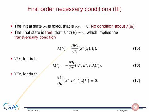
• The initial state x0 is fixed, that is δx0 = 0. No condition about λ(t0).• The final state is free, that is δx(tf ) 6= 0, which implies the
transversality condition
λ(tf ) =∂Kf
∂x(x∗(tf ), tf ). (15)
• ∀δx , leads to
λ(t) = −∂H∂x
(x∗,u∗, t , λ(t)). (16)
• ∀δx , leads to∂H∂u
(x∗,u∗, t , λ(t)) = 0. (17)
Introduction 12 / 55 M. Jungers
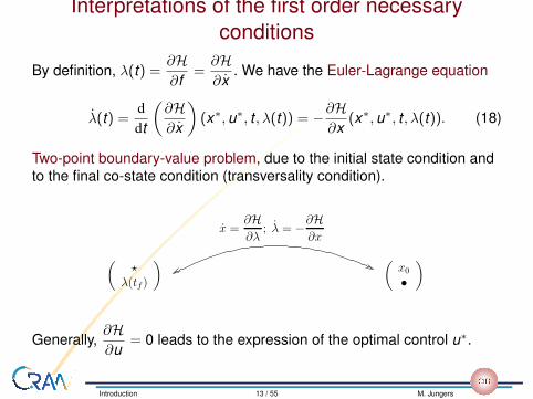
Interpretations of the first order necessaryconditions
By definition, λ(t) =∂H∂f
=∂H∂x
. We have the Euler-Lagrange equation
λ(t) =ddt
(∂H∂x
)(x∗,u∗, t , λ(t)) = −∂H
∂x(x∗,u∗, t , λ(t)). (18)
Two-point boundary-value problem, due to the initial state condition andto the final co-state condition (transversality condition).
!!
"(tf)
" !x0
•
"
x =#H#"
; " = !#H#x
1
Generally,∂H∂u
= 0 leads to the expression of the optimal control u∗.
Introduction 13 / 55 M. Jungers
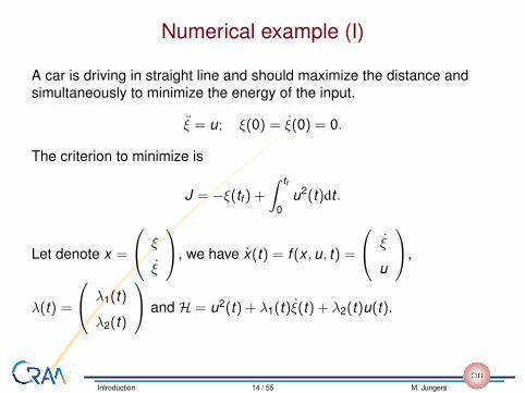
Numerical example (I)
A car is driving in straight line and should maximize the distance andsimultaneously to minimize the energy of the input.
ξ = u; ξ(0) = ξ(0) = 0.
The criterion to minimize is
J = −ξ(tf ) +
∫ tf
0u2(t)dt .
Let denote x =
ξ
ξ
, we have x(t) = f (x ,u, t) =
ξ
u
,
λ(t) =
λ1(t)
λ2(t)
and H = u2(t) + λ1(t)ξ(t) + λ2(t)u(t).
Introduction 14 / 55 M. Jungers
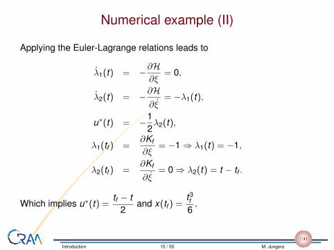
Numerical example (II)
Applying the Euler-Lagrange relations leads to
λ1(t) = −∂H∂ξ
= 0,
λ2(t) = −∂H∂ξ
= −λ1(t),
u∗(t) = −12λ2(t),
λ1(tf ) =∂Kf
∂ξ= −1⇒ λ1(t) = −1,
λ2(tf ) =∂Kf
∂ξ= 0⇒ λ2(t) = t − tf .
Which implies u∗(t) =tf − t
2and x(tf ) =
t3f6
.
Introduction 15 / 55 M. Jungers
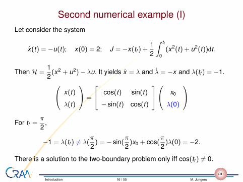
Second numerical example (I)Let consider the system
x(t) = −u(t); x(0) = 2; J = −x(tf ) +12
∫ tf
0(x2(t) + u2(t))dt .
Then H =12
(x2 + u2)− λu. It yields x = λ and λ = −x and λ(tf ) = −1.
x(t)
λ(t)
=
cos(t) sin(t)
− sin(t) cos(t)
x0
λ(0)
For tf =π
2,
−1 = λ(tf ) 6= λ(π
2) = − sin(
π
2)x0 + cos(
π
2)λ(0) = −2.
There is a solution to the two-boundary problem only iff cos(tf ) 6= 0.
Introduction 16 / 55 M. Jungers

Third numerical example (I)
Let consider the system with two inputs
x(t) = u1(t) + u2(t); x(0) = 0.
The criterion to minimize is
J = −x(tf ) +
∫ tf
0(u2
1(t)− u22(t))dt .
Then H = u21(t)− u2
2(t) + λ(t)[u1(t) + u2(t)].
Introduction 17 / 55 M. Jungers

Third numerical example (II)Applying the Euler-Lagrange relations leads to
λ(t) = −∂H∂x
= 0 ⇒ λ(t) = Cste,
∂H∂u1
= 0 ⇒ u1(t) = −12λ,
∂H∂u2
= 0 ⇒ u2(t) = +12λ,
λ(tf ) =∂(−xf )
∂xf= −1.
That implies λ(t) = −1, u1(t) = −u2(t) = −12
and x(t) = 0 and finallyJ∗ = 0. Nevertheless for u1(t) = u2(t) = 1, we have x(t) = 2t andJ = −2tf < 0 = J∗. J∗ is not the minimum, but a saddle-point.
Further necessary conditions are required.
Introduction 18 / 55 M. Jungers
Second order necessary conditions
The solution consists in a mimimum and not only in an extremum.
∂2H∂u2 > 0.
Link with the convexity of the criterion and implicit function theorem.
Introduction 19 / 55 M. Jungers
Formulation of the problem
Motivation
Variational approach : Euler-Lagrange equation
Pontryaguin Minimum Principle
Dynamic Programming
Linear Quadratic Control Problem
Conclusion and Open Questions
Introduction 20 / 55 M. Jungers
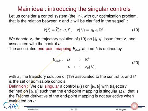
Main idea : introducing the singular controlsLet us consider a control system (the link with our optimization problem,that is the relation between x and z will be clarified in the sequel) :
z(t) = f (z,u, t), z(t0) = z0 ∈ R`. (19)
We denote zu the trajectory solution of (19) on [t0, tf ] issue from z0 andassociated with the control u.The associated end-point mapping Ez0,tf at time tf is defined by
Ez0,tf : U −→ R`
u 7−→ zu(tf ),(20)
with zu the trajectory solution of (19) associated to the control u, and Uis the set of admissible controls.Definition : We call singular a control u(t) on [t0, tf ] with trajectorydefined on [t0, tf ] such that the end-point mapping is singular at u, that isthe Fréchet derivative of the end-point mapping is not surjective whenevaluated on u.
Introduction 21 / 55 M. Jungers
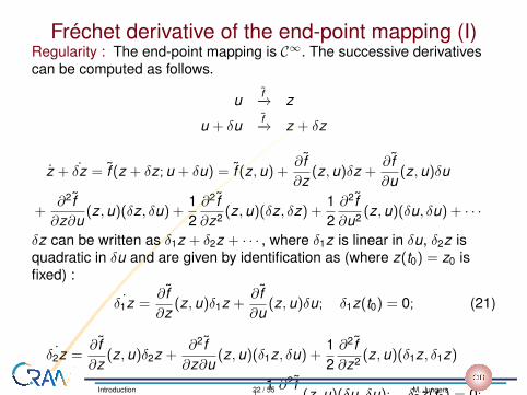
Fréchet derivative of the end-point mapping (I)Regularity : The end-point mapping is C∞. The successive derivativescan be computed as follows.
u f−→ z
u + δu f−→ z + δz
z + ˙δz = f (z + δz; u + δu) = f (z,u) +∂ f∂z
(z,u)δz +∂ f∂u
(z,u)δu
+∂2 f∂z∂u
(z,u)(δz, δu) +12∂2 f∂z2 (z,u)(δz, δz) +
12∂2 f∂u2 (z,u)(δu, δu) + · · ·
δz can be written as δ1z + δ2z + · · · , where δ1z is linear in δu, δ2z isquadratic in δu and are given by identification as (where z(t0) = z0 isfixed) :
˙δ1z =∂ f∂z
(z,u)δ1z +∂ f∂u
(z,u)δu; δ1z(t0) = 0; (21)
˙δ2z =∂ f∂z
(z,u)δ2z +∂2 f∂z∂u
(z,u)(δ1z, δu) +12∂2 f∂z2 (z,u)(δ1z, δ1z)
+12∂2 f∂u2 (z,u)(δu, δu); δ2z(t0) = 0;Introduction 22 / 55 M. Jungers
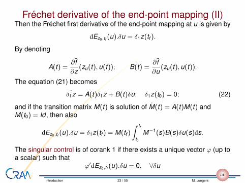
Fréchet derivative of the end-point mapping (II)Then the Fréchet first derivative of the end-point mapping at u is given by
dEz0,tf (u).δu = δ1z(tf ).
By denoting
A(t) =∂ f∂z
(zu(t),u(t)); B(t) =∂ f∂u
(zu(t),u(t));
The equation (21) becomes
˙δ1z = A(t)δ1z + B(t)δu; δ1z(t0) = 0; (22)
and if the transition matrix M(t) is solution of M(t) = A(t)M(t) andM(t0) = Id , then also
dEz0,tf (u).δu = δ1z(tf ) = M(tf )∫ tf
t0M−1(s)B(s)δu(s)ds.
The singular control is of corank 1 if there exists a unique vector ϕ (up toa scalar) such that
ϕ′dEz0,tf (u).δu = 0, ∀δu
Introduction 23 / 55 M. Jungers
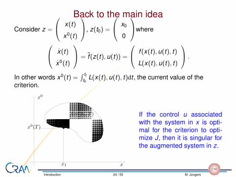
Back to the main ideaConsider z =
x(t)
x0(t)
, z(t0) =
x0
0
where
x(t)
x0(t)
= f (z(t),u(t)) =
f (x(t),u(t), t)
L(x(t),u(t), t)
.
In other words x0(t) =∫ tf
t0L(x(t),u(t), t)dt , the current value of the
criterion.
102 CHAPITRE 7. PRINCIPE DU MAXIMUM DE PONTRYAGIN
et notons x = (x, x0), f = (f, f0). Le problème revient donc à chercher unetrajectoire solution de (7.3) joignant les points x0 = (x0, 0) et x1 = (x1, x
0(T )),et minimisant la dernière coordonnée x0(T ).
L’ensemble des états accessibles à partir de x0 pour le système (7.3) estAcc(x0, T ) =
!u(·)
x(T, x0, u).
Le lemme crucial est alors le suivant.
Lemme 7.1.1. Si le contrôle u associé au système de contrôle (7.1) est optimalpour le coût (7.2), alors il est singulier sur [0, T ] pour le système augmenté(7.3).
Démonstration. Notons x la trajectoire associée, solution du système augmenté(7.3), issue de x0 = (x0, 0). Le contrôle u étant optimal pour le coût (7.2), il enrésulte que le point x(T ) appartient à la frontière de l’ensemble Acc(x0, T ) (voirfigure 7.1). En e!et sinon, il existerait un voisinage du point x(T ) = (x1, x
0(T ))dans Acc(x0, T ) contenant un point y(T ) solution du système (7.3) et tel que l’onait y0(T ) < x0(T ), ce qui contredirait l’optimalité du contrôle u. Par conséquent,d’après la proposition 5.3.1, le contrôle u est un contrôle singulier pour le systèmeaugmenté (7.3) sur [0, T ].
x
x0
x1
x0(T )
Acc(x0, T )
Fig. 7.1 – Ensemble accessible augmenté.
Dans la situation du lemme, d’après la proposition 5.3.4, il existe une ap-plication p : [0, T ] !" IRn+1 \ {0} telle que (x, p, u) soit solution du systèmehamiltonien
˙x(t) =!H
!p(t, x(t), p(t), u(t)), ˙p(t) = !!H
!x(t, x(t), p(t), u(t)), (7.4)
!H
!u(t, x(t), p(t), u(t)) = 0 (7.5)
où H(t, x, p, u) = #p, f(t, x, u)$.
If the control u associatedwith the system in x is opti-mal for the criterion to opti-mize J, then it is singular forthe augmented system in z.
Introduction 24 / 55 M. Jungers
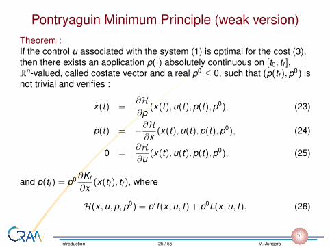
Pontryaguin Minimum Principle (weak version)Theorem :If the control u associated with the system (1) is optimal for the cost (3),then there exists an application p(·) absolutely continuous on [t0, tf ],Rn-valued, called costate vector and a real p0 ≤ 0, such that (p(tf ),p0) isnot trivial and verifies :
x(t) =∂H∂p
(x(t),u(t),p(t),p0), (23)
p(t) = −∂H∂x
(x(t),u(t),p(t),p0), (24)
0 =∂H∂u
(x(t),u(t),p(t),p0), (25)
and p(tf ) = p0 ∂Kf
∂x(x(tf ), tf ), where
H(x ,u,p,p0) = p′f (x ,u, t) + p0L(x ,u, t). (26)
Introduction 25 / 55 M. Jungers

Pontryaguin Minimum Principle : sketch of proof
ϕ′dEz0,tf (u).δu = 0
implies that
ϕ′M(tf )M−1(s)B(s) = 0 almost everywhere on [t0, tf ].
Let define
p(t)
p0(t)
′
= ϕ′M(tf )M−1(t). Then
•
p(tf )
p0(tf )
= ϕ not trivial !
• (p′(t); p0) = −(p′(t); p0)
∂f∂x
0∂L∂x
0
.
•
p(t)
p0(t)
′
B(t) = 0 =
p(t)
p0(t)
′
∂f∂u∂L∂u
.
Introduction 26 / 55 M. Jungers

Pontryaguin Minimum Principle (strong version)
Theorem :If the control u U-valued associated with the system (1) is optimal for thecost (3), then there exists an application p(·) absolutely continuous on[t0, tf ], Rn-valued, called costate vector and a real p0 ≤ 0, such that(p(tf ),p0) is not trivial and verifies :
x(t) =∂H∂p
(x(t),u(t),p(t),p0), (27)
p(t) = −∂H∂x
(x(t),u(t),p(t),p0), (28)
⇒ u∗(t) = argminu∈UH(x(t),u(t),p(t),p0), (29)
and p(tf ) = p0 ∂Kf
∂x(x(tf ), tf ), where
H(x ,u,p,p0) = p′f (x ,u, t) + p0L(x ,u, t). (30)
Introduction 27 / 55 M. Jungers
Pontryaguin Minimum Principle (strong version)
Interpretation :More difficult to prove. A larger set of admissible controls (u not anymorecontinuous) is considered. PMP and Euler-Lagrange Theorem differ onthe fact that the PMP tells us that the Hamiltonian is minimized at theoptimal trajectory and that it is also applicable when the minimum isattained at the boundary of U . See also that p0 cannot be null.
Introduction 28 / 55 M. Jungers

Numerical exampleLet us consider the system x = u, with the criterion
∫ tft0
x(t)dt − 2x(tf )and the constraint ‖u‖ ≤ 1. We have the Hamiltonian H = x + pu,leading to p(t) = −1, p(tf ) = −2. One gets p(t) = tf − t − 2. Furthermore
u∗(t) = argminu(t)∈[−1,1](x(t) + p(t)u(t)) =
1 if p(t) < 0
undefined if p(t) = 0
−1 if p(t) > 0.
0 0.5 1 1.5 2 2.5 3 3.5 4 4.5 51
0
1
t
u* (t) p
our t
f=1
0 0.5 1 1.5 2 2.5 3 3.5 4 4.5 51
0
1
t
u* (t) p
our t
f=2
0 0.5 1 1.5 2 2.5 3 3.5 4 4.5 51
0
1
t
u* (t) p
our t
f=3
0 0.5 1 1.5 2 2.5 3 3.5 4 4.5 51
0
1
t
u* (t) p
our t
f=4
If tf ≤ 2 : u∗(t) = 1.
If tf ≥ 2 :
u∗(t) =
1 if tf − 2 < t ≤ tf ,
−1 if 0 ≤ t < tf − 2.
Introduction 29 / 55 M. Jungers
Formulation of the problem
Motivation
Variational approach : Euler-Lagrange equation
Pontryaguin Minimum Principle
Dynamic Programming
Linear Quadratic Control Problem
Conclusion and Open Questions
Introduction 30 / 55 M. Jungers
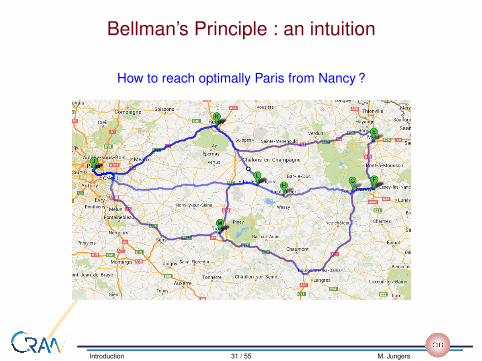
Bellman’s Principle : an intuition
How to reach optimally Paris from Nancy ?
Introduction 31 / 55 M. Jungers
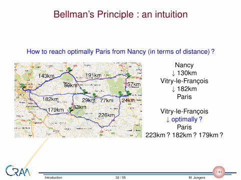
Bellman’s Principle : an intuition
How to reach optimally Paris from Nancy (in terms of distance) ?
Nancy↓ 130km
Vitry-le-François↓ 182km
Paris
Vitry-le-François↓ optimally ?
Paris223km ? 182km ? 179km ?
Introduction 32 / 55 M. Jungers
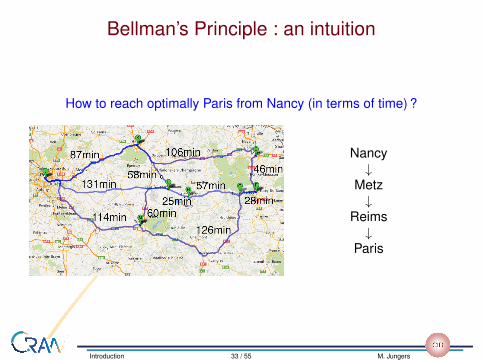
Bellman’s Principle : an intuition
How to reach optimally Paris from Nancy (in terms of time) ?
Nancy↓
Metz↓
Reims↓
Paris
Introduction 33 / 55 M. Jungers

Bellman’s Principle : sufficient conditions ofoptimality
Dynamic Programming (DP) is a commonly used method of optimallysolving complex problems by breaking them down into simpler problems.
Principle : An optimal policy has the property that whatever the initialstate and initial decision are, the remaining decisions must constitute anoptimal policy with regard to the state resulting from the first decision.
CA
B
1
“it’s better to be smart from the beginning, than to be stupid for a timeand then become smart”
Introduction 34 / 55 M. Jungers

Value function (I)Let us define the value function as the optimal criterion on the restrictedtime-horizon : [t , tf ], always ending at tf and starting at time t with theinitial condition x(t) :
V (t , x(t)) = J∗|[t,tf ] = minu|[t,tf ]
(Kf (x(tf ), tf ) +
∫ tf
tL(x(s),u(s), s)ds
). (31)
We have (with the minimum taken under x(t) = f (x(t),u(t), t))
V (t , x(t)) = minu|[t,tf ]
(∫ t+∆t
tL(x(s),u(s), s)ds
︸ ︷︷ ︸Cost between [t, t + ∆t]
+ V (t + ∆t , x(t + ∆t))︸ ︷︷ ︸Optimal between [t + ∆t, tf ] from x(t + ∆t)
).
x = x(t)
x(t + !t)
t t + !t tf
x = x(t)
1
Introduction 35 / 55 M. Jungers
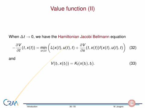
Value function (II)
When ∆t → 0, we have the Hamiltonian Jacobi Bellmann equation
−∂V∂t
(t , x(t)) = minu∈U
(L(x(t),u(t), t) +
∂V∂x
(t , x(t))f (x(t),u(t), t))
(32)
andV (tf , x(tf )) = Kf (x(tf ), tf ). (33)
Introduction 36 / 55 M. Jungers

Dynamic Programming
Let V (t , x) defined by (31), and assume that both partial derivatives of
V (t , x) exist,∂V∂x
is continuous and moreoverddt
V (t , x(t)) exists, then
−∂V∂t
(t , x(t)) = minu∈U
(L(x(t),u(t), t) +
∂V∂x
(t , x(t))f (x(t),u(t), t))
; (34)
V (tf , x(tf )) = Kf (x(tf ), tf ) (35)
and
u∗(t) = argminu∈U
(L(x(t),u(t), t) +
∂V∂x
(t , x(t))f (x(t),u(t), t))
(36)
Introduction 37 / 55 M. Jungers

Numerical example
Let consider x(t) = x(t)u(t), with u ∈ [−1,1] and J = x(tf ). If x0 > 0,then u = −1 and if x0 < 0, then u = 1. If x0 = 0, J = 0.
V (t , x) =
e−(tf−t) if x > 0,
e(tf−t) if x < 0,
0 if x = 0,
No C1 solution to HJB equation. Viscosity Solution for HJB equation isrequired.
Introduction 38 / 55 M. Jungers

Formulation of the problem
Motivation
Variational approach : Euler-Lagrange equation
Pontryaguin Minimum Principle
Dynamic Programming
Linear Quadratic Control Problem
Conclusion and Open Questions
Introduction 39 / 55 M. Jungers

Linear Quadratic control problem
System :
x(t) = Ax(t) + Bu(t), x ∈ Rn, u ∈ Rr .
x(t0) = x0.
Criterion to minimize :
J = x ′(tf )Kf x(tf ) +12
∫ tf
t0(x ′(t)Qx(t) + u′(t)Ru(t)) dt
Assumptions :Q = Q′ ≥ 0n, R = R′ > 0r .
Introduction 40 / 55 M. Jungers
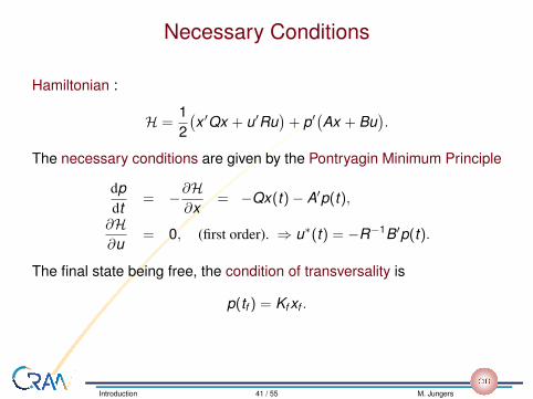
Necessary Conditions
Hamiltonian :
H =12(x ′Qx + u′Ru
)+ p′
(Ax + Bu
).
The necessary conditions are given by the Pontryagin Minimum Principle
dpdt
= −∂H∂x
= −Qx(t)− A′p(t),
∂H∂u
= 0, (first order). ⇒ u∗(t) = −R−1B′p(t).
The final state being free, the condition of transversality is
p(tf ) = Kf xf .
Introduction 41 / 55 M. Jungers

Two Boundary Problem
Resolve x
p
= H
x
p
=
A −S
−Q −A′
x
p
where S = BR−1B′, with the two boundary conditions
x(t0) = x0, p(tf ) = Kf x(tf ).
How to solve this kind of problem ?
Introduction 42 / 55 M. Jungers
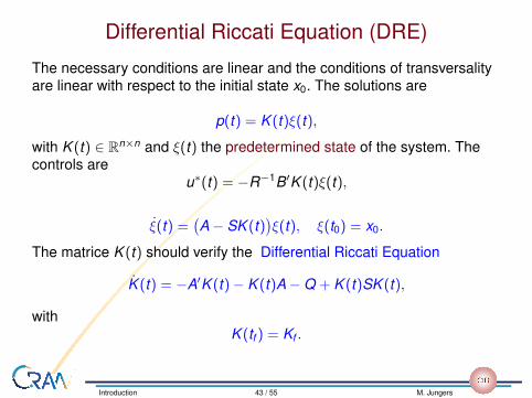
Differential Riccati Equation (DRE)
The necessary conditions are linear and the conditions of transversalityare linear with respect to the initial state x0. The solutions are
p(t) = K (t)ξ(t),
with K (t) ∈ Rn×n and ξ(t) the predetermined state of the system. Thecontrols are
u∗(t) = −R−1B′K (t)ξ(t),
ξ(t) =(A− SK (t)
)ξ(t), ξ(t0) = x0.
The matrice K (t) should verify the Differential Riccati Equation
K (t) = −A′K (t)− K (t)A−Q + K (t)SK (t),
withK (tf ) = Kf .
Introduction 43 / 55 M. Jungers
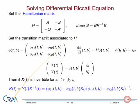
Solving Differential Riccati EquationSet the Hamiltonian matrix
H =
A −S
−Q −A′
, where S = BR−1B′.
Set the transition matrix associated to H
φ(t , tf ) =
φ11(t , tf ) φ12(t , tf )
φ21(t , tf ) φ22(t , tf )
,
dφdt
(t , tf ) = Hφ(t , tf ), φ(tf , tf ) = I2n.
X (t)
Y (t)
= φ(t , tf )
In
Kf
Then if X (t) is invertible for all t ∈ [t0, tf ]
K (t) = Y (t)X−1(t) =(φ21(t , tf ) + φ22(t , tf )Kf
)(φ11(t , tf ) + φ12(t , tf )Kf
)−1.
Introduction 44 / 55 M. Jungers

ExampleMinimize
J = Kf x2(1) +
∫ tf
0
(x2(t) + u2(t)
)dt ,
under the constraint
x(t) = u(t), x(0) = x0 = 1.
H =
0 −1
−1 0
⇒ φ(t , tf ) =
12
e−(t−tf ) + e(t−tf ) e−(t−tf ) − e(t−tf )
e−(t−tf ) − e(t−tf ) e−(t−tf ) + e(t−tf )
So we obtain
K (t , tf ) =(1− e2(t−tf )) + Kf (1 + e2(t−tf ))
(1 + e2(t−tf )) + Kf (1− e2(t−tf ))
Introduction 45 / 55 M. Jungers
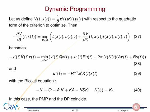
Dynamic Programming
Let us define V (t , x(t)) =12
x ′(t)K (t)x(t) with respect to the quadraticform of the criterion to optimize. Then
−∂V∂t
(t , x(t)) = minu∈U
(L(x(t),u(t), t) +
∂V∂x
(t , x(t))f (x(t),u(t), t))
(37)
becomes
−x ′(t)K (t)x(t) = minu∈U
(x ′(t)Qx(t) + u′(t)Ru(t) + 2x ′(t)K (t)(Ax(t) + Bu(t)))
(38)and
u∗(t) = −R−1B′K (t)x(t) (39)
with the Riccati equation :
−K = Q + A′K + KA− KSK ; K (tf ) = Kf . (40)
In this case, the PMP and the DP coincide.
Introduction 46 / 55 M. Jungers

Explosion in finite time
The Riccati equation may have no solution on the interval [t0, tf ], due toexplosion in finite time (which are characteristic of nonlinear equations).
For examplek(t) = 1 + k2(t), k(0) = 0 (41)
has a solution t 7→ tan(t), which exploses in finite time at t =π
2.
Introduction 47 / 55 M. Jungers
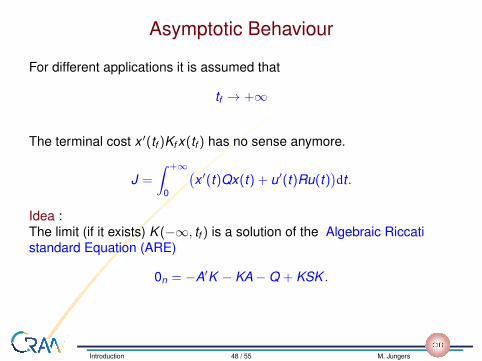
Asymptotic Behaviour
For different applications it is assumed that
tf → +∞
The terminal cost x ′(tf )Kf x(tf ) has no sense anymore.
J =
∫ +∞
0
(x ′(t)Qx(t) + u′(t)Ru(t)
)dt .
Idea :The limit (if it exists) K (−∞, tf ) is a solution of the Algebraic Riccatistandard Equation (ARE)
0n = −A′K − KA−Q + KSK .
Introduction 48 / 55 M. Jungers
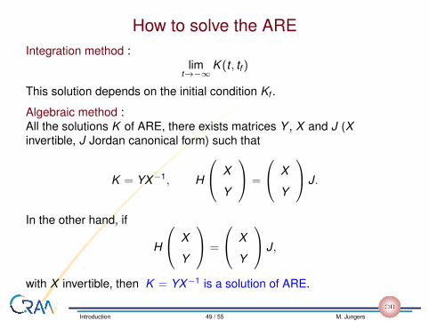
How to solve the AREIntegration method :
limt→−∞
K (t , tf )
This solution depends on the initial condition Kf .
Algebraic method :All the solutions K of ARE, there exists matrices Y , X and J (Xinvertible, J Jordan canonical form) such that
K = YX−1, H
X
Y
=
X
Y
J.
In the other hand, if
H
X
Y
=
X
Y
J,
with X invertible, then K = YX−1 is a solution of ARE.
Introduction 49 / 55 M. Jungers
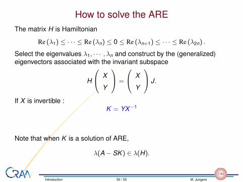
How to solve the AREThe matrix H is Hamiltonian
Re (λ1) ≤ · · · ≤ Re (λn) ≤ 0 ≤ Re (λn+1) ≤ · · · ≤ Re (λ2n) .
Select the eigenvalues λ1, · · · , λn and construct by the (generalized)eigenvectors associated with the invariant subspace
H
X
Y
=
X
Y
J.
If X is invertible :K = YX−1
Note that when K is a solution of ARE,
λ(A− SK ) ∈ λ(H).
Introduction 50 / 55 M. Jungers

Example
integration method
limtf→+∞
K (t , tf ) = +1
This limit does not depend on Kf .
algebraic method
H = VDV−1, V =
1 1
1 −1
, D =
−1 0
0 1
The only one stabilizing solution is given by the eigenvalue −1 and the
eigenvector
1
1
.
K = YX−1 = 1 A− SK = −1.
Introduction 51 / 55 M. Jungers
Formulation of the problem
Motivation
Variational approach : Euler-Lagrange equation
Pontryaguin Minimum Principle
Dynamic Programming
Linear Quadratic Control Problem
Conclusion and Open Questions
Introduction 52 / 55 M. Jungers
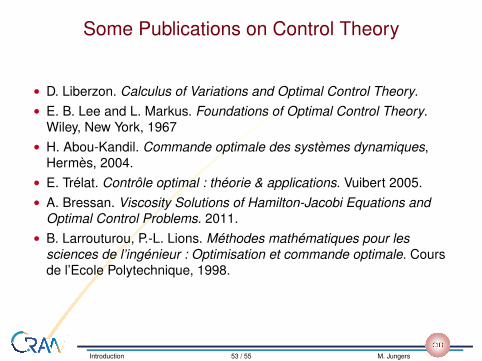
Some Publications on Control Theory
• D. Liberzon. Calculus of Variations and Optimal Control Theory.• E. B. Lee and L. Markus. Foundations of Optimal Control Theory.
Wiley, New York, 1967• H. Abou-Kandil. Commande optimale des systèmes dynamiques,
Hermès, 2004.• E. Trélat. Contrôle optimal : théorie & applications. Vuibert 2005.• A. Bressan. Viscosity Solutions of Hamilton-Jacobi Equations and
Optimal Control Problems. 2011.• B. Larrouturou, P.-L. Lions. Méthodes mathématiques pour les
sciences de l’ingénieur : Optimisation et commande optimale. Coursde l’Ecole Polytechnique, 1998.
Introduction 53 / 55 M. Jungers
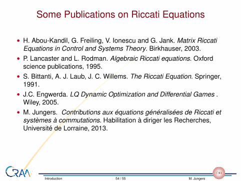
Some Publications on Riccati Equations
• H. Abou-Kandil, G. Freiling, V. Ionescu and G. Jank. Matrix RiccatiEquations in Control and Systems Theory. Birkhauser, 2003.
• P. Lancaster and L. Rodman. Algebraic Riccati equations. Oxfordscience publications, 1995.
• S. Bittanti, A. J. Laub, J. C. Willems. The Riccati Equation. Springer,1991.
• J.C. Engwerda. LQ Dynamic Optimization and Differential Games .Wiley, 2005.
• M. Jungers. Contributions aux équations généralisées de Riccati etsystèmes à commutations. Habilitation à diriger les Recherches,Université de Lorraine, 2013.
Introduction 54 / 55 M. Jungers