HAL Id: inria-00630050https://hal.inria.fr/inria-00630050

Submitted on 7 Oct 2011

HAL is a multi-disciplinary open accessarchive for the deposit and dissemination of sci-entific research documents, whether they are pub-lished or not. The documents may come fromteaching and research institutions in France orabroad, or from public or private research centers.

L’archive ouverte pluridisciplinaire HAL, estdestinée au dépôt et à la diffusion de documentsscientifiques de niveau recherche, publiés ou non,émanant des établissements d’enseignement et derecherche français ou étrangers, des laboratoirespublics ou privés.

Tutorial on Differential GamesMarc Quincampoix

To cite this version:Marc Quincampoix. Tutorial on Differential Games. SADCO Summer School 2011 - Optimal Control,Sep 2011, London, United Kingdom. <inria-00630050>

Differential Games III

Marc QuincampoixUniversite de Bretagne Occidentale ( Brest-France)

SADCO, London, September 2011

Contents

1. I Introduction: A Pursuit Game and Isaacs Theory

2. II Strategies

3. III Dynamic Programming Principle

4. IV Existence of Value, Viscosity Solutions

5. I V Games on the space of measures, Incomplete in-formation

Joint Work P. Cardaliaguet , M.Q

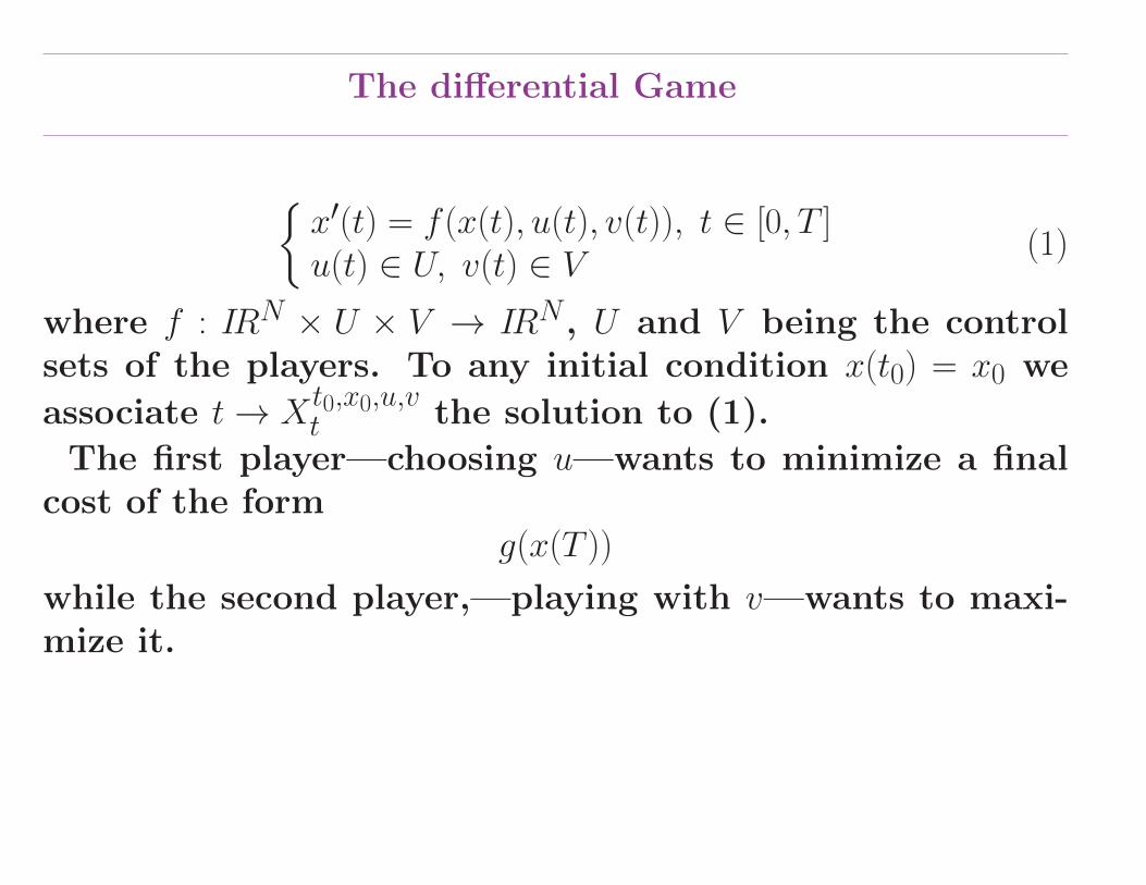
The differential Game

{x′(t) = f (x(t), u(t), v(t)), t ∈ [0, T ]u(t) ∈ U, v(t) ∈ V (1)

where f : IRN × U × V → IRN , U and V being the controlsets of the players. To any initial condition x(t0) = x0 we

associate t→ Xt0,x0,u,vt the solution to (1).

The first player—choosing u—wants to minimize a finalcost of the form

g(x(T ))

while the second player,—playing with v—wants to maxi-mize it.

the state-space x0 is only unperfectly known by the play-ers : they only know that the initial position is randomlydistributed under some fixed probability measure µ0. Bothplayers are assumed to know this probability µ0, and havea perfect knowledge of the control of the other player.

So the ”lack” of information is very specific :

• it is symmetric for both player

• it is only concerned with the current position of thegame.

We denote by M the Borel probability measures µ s.t.∫IRN|x|2dµ(x) < +∞ .

Assumptions

(i) U and V are compact subsets of some finitedimensional spaces

(ii) f : IRN × U × V → IRN is continuous andLipschitz continuous with respect to

(iii) ∀(x, u, v), |f (x, u, v)| ≤M

(iv) g : IRN → IR is Lipschitz continuous and bounded

(2)

U(t0) = {u : [t0, T ]→ U, Lebesgue measurable}V(t0) = {v : [t0, T ]→ V, Lebesgue measurable}

Strategies

Definition 1 A NAD strategy is a map α : V(t0) → U(t0)such that there is some τ > 0 such that ∀t,∀v1, v2 ∈ V(t0), v1 = v2 on [t0, t] ⇒ α(v1) = α(v2) on [t0, t + τ ].

A(t0) is the set of such α. Symmetrically, B(t0) is the setof NAD strategies β : U(t0)→ V(t0) for the second player.

Lemma 2 ∀(α, β) ∈ A(t0)× B(t0), ∃!(u0, v0) ∈ U(t0)× V(t0),

α(v0) = u0 and β(u0) = v0 .

Xt0,x,α,βt := X

t0,x,u0,v0t ∀t ∈ [t0, T ] .

Payoffs and Values

g : IRN 7→ IR which is Lipschitz and bounded. For any(t0, µ0) ∈ [0, T )×M and for any (u, v) ∈ U(t0)× V(t0) we set

J(t0, µ0, u, v) =

∫IRN

g(Xt0,x,u,vT

)dµ(x) .

For any pair of strategies (α, β) ∈ A(t0)× B(t0), we define

J(t0, µ0, α, β) = J(t0, µ0, u0, v0)

where (u0, v0) ∈ U(t0) × V(t0) is associated to (α, β) by theLemma

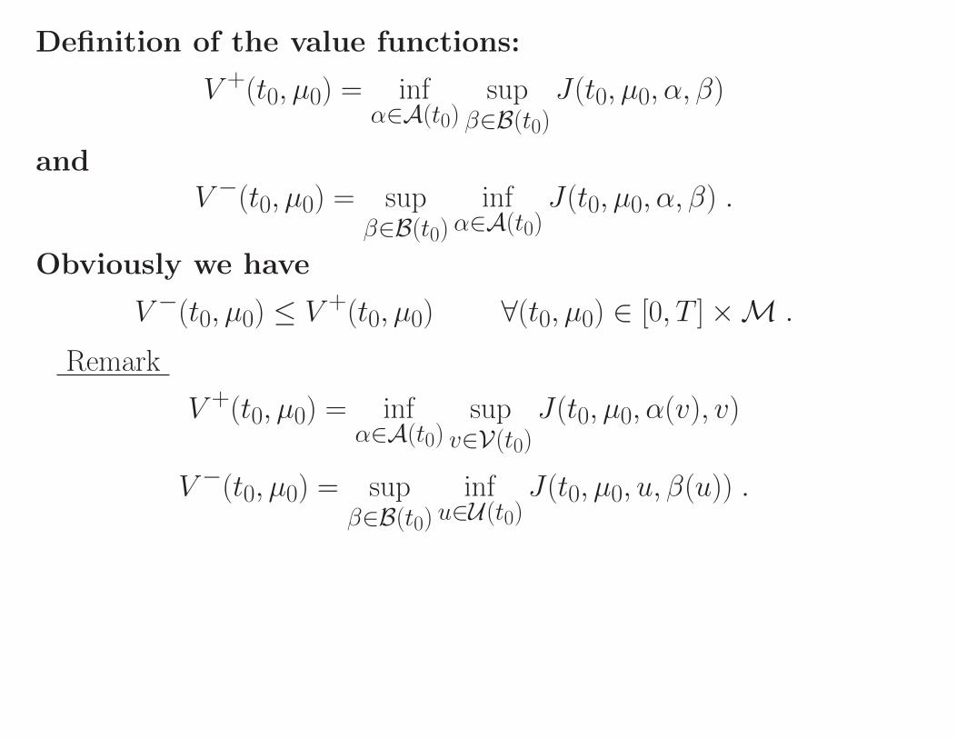
Definition of the value functions:

V +(t0, µ0) = infα∈A(t0)

supβ∈B(t0)

J(t0, µ0, α, β)

andV −(t0, µ0) = sup

β∈B(t0)inf

α∈A(t0)J(t0, µ0, α, β) .

Obviously we have

V −(t0, µ0) ≤ V +(t0, µ0) ∀(t0, µ0) ∈ [0, T ]×M .

Remark

V +(t0, µ0) = infα∈A(t0)

supv∈V(t0)

J(t0, µ0, α(v), v)

V −(t0, µ0) = supβ∈B(t0)

infu∈U(t0)

J(t0, µ0, u, β(u)) .

Preliminaries on Probability Measures

For µ ∈M, we denote by L2µ(IRN , IR) (resp. L2

µ(IRN , IRN ))

the set of µ−measurables maps p : IRN → IR (resp. p :IRN → IRN) such that ‖p‖L2

µ:=∫IRN |p|

2dµ < +∞

For µ ∈ M and ϕ : IRN → IRN a Borel measurable withlinear growth, ϕ]µ is the push-forward of µ by ϕ,

ϕ]µ(A) = µ(ϕ−1(A)

)∀A ⊂ IRN , Borel measurable

or, equivalently, such that, ∀f : IRN → IR, Borel measurableand bounded,∫

IRNfd(ϕ]µ) =

∫IRN

f (ϕ(x))dµ(x) .

Wasserstein Distance cf book of Villani

d(µ, ν) = inf

(∫

IR2N|x− y|2dγ

)12

(3)

where the infimum is taken over all the probability mea-sures γ in IR2N such that

π1]γ = µ and π2]γ = ν , (4)

π1 and π2 being respectively the projections on the firstand the second coordinates: π1(x, y) = x and π2(x, y) = y.A measure γ satisfying (4) is an admissible transport planfrom µ to ν. The optimal γ are called optimal plans.

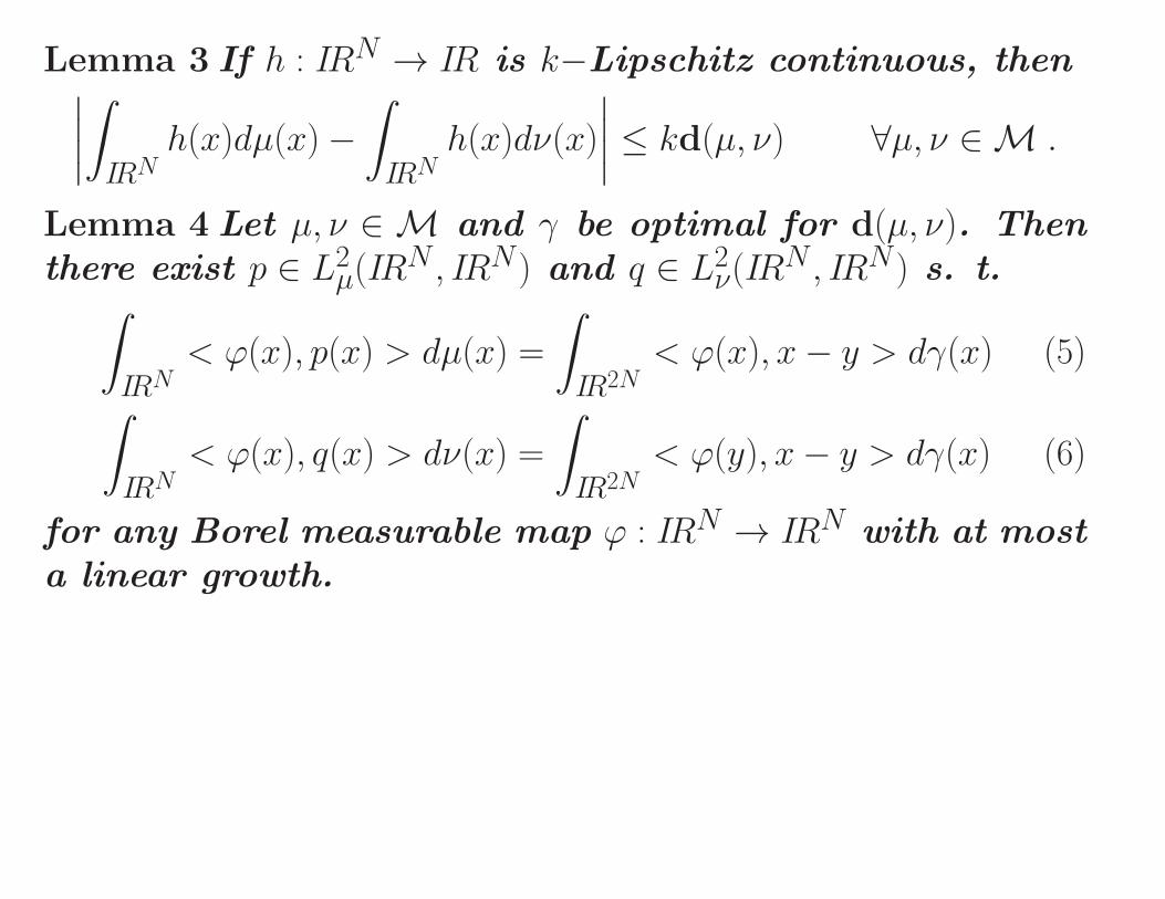
Lemma 3 If h : IRN → IR is k−Lipschitz continuous, then∣∣∣∣∫IRN

h(x)dµ(x)−∫IRN

h(x)dν(x)

∣∣∣∣ ≤ kd(µ, ν) ∀µ, ν ∈M .

Lemma 4 Let µ, ν ∈ M and γ be optimal for d(µ, ν). Thenthere exist p ∈ L2

µ(IRN , IRN ) and q ∈ L2ν(IRN , IRN ) s. t.∫

IRN< ϕ(x), p(x) > dµ(x) =

∫IR2N

< ϕ(x), x− y > dγ(x) (5)∫IRN

< ϕ(x), q(x) > dν(x) =

∫IR2N

< ϕ(y), x− y > dγ(x) (6)

for any Borel measurable map ϕ : IRN → IRN with at mosta linear growth.

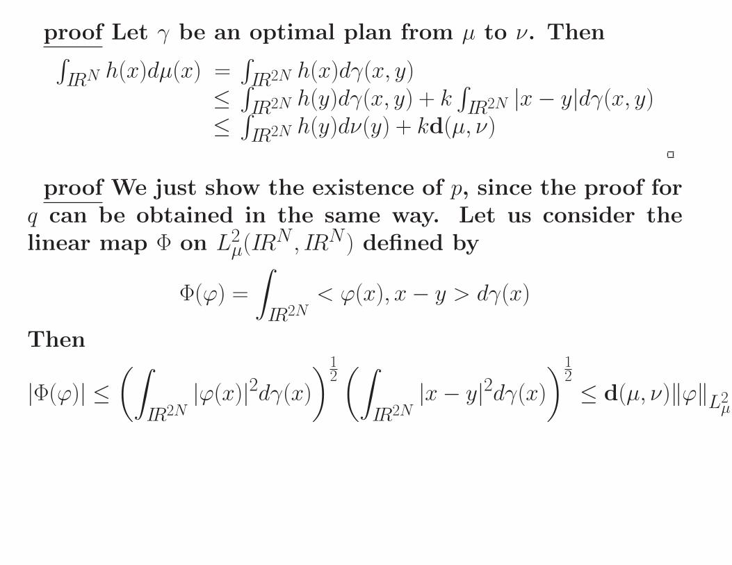
proof Let γ be an optimal plan from µ to ν. Then∫IRN h(x)dµ(x) =

∫IR2N h(x)dγ(x, y)

≤∫IR2N h(y)dγ(x, y) + k

∫IR2N |x− y|dγ(x, y)

≤∫IR2N h(y)dν(y) + kd(µ, ν)

proof We just show the existence of p, since the proof forq can be obtained in the same way. Let us consider thelinear map Φ on L2

µ(IRN , IRN ) defined by

Φ(ϕ) =

∫IR2N

< ϕ(x), x− y > dγ(x)

Then

|Φ(ϕ)| ≤(∫

IR2N|ϕ(x)|2dγ(x)

)12(∫

IR2N|x− y|2dγ(x)

)12≤ d(µ, ν)‖ϕ‖L2

µ

for any ϕ ∈ L2µ(IRN , IRN ). Therefore Φ is bounded on L2

µ(IRN , IRN ),

whence the existence of p ∈ L2µ(IRN , IRN ) from Riesz Rep-

resentation Theorem.

Regularity of the Values

Proposition 5 The value functions V + and V − are Lips-chitz continuous.

proof for V +

We shall first prove that the values are Lipschitz contin-uous with respect to the second variable. Fix t0 ∈ [0, T ],µ0 ∈ M, ν0 ∈ M and ε > 0. There exists an nonanticipativestrategy αε ∈ A(t0) such that

V +(t0, ν0) ≤ supβ∈B(t0)

J(t0, ν0, αε, β) ≤ V +(t0, ν0) + ε.

HenceV +(t0, µ0)− V +(t0, ν0) ≤

ε + supβ∈B(t0)

J(t0, µ0, αε, β)− supβ∈B(t0)

J(t0, ν0, αε, β)

≤ 2ε + J(t0, µ0, αε, βε)− J(t0, ν0, αε, βε)

where βε ∈ B(t0) is such that

supβ∈B(t0)

J(t0, µ0, αε, β)−ε ≤ J(t0, µ0, αε, βε) ≤ supβ∈B(t0)

J(t0, µ0, αε, β).

ThusV +(t0, µ0)− V +(t0, ν0) ≤

2ε +

∫IRN

g(Xt0,x,αε,βεT

)dµ0(x)−

∫IRN

g(Xt0,x,αε,βεT

)dν0(x)

≤ k2ekTd(µ0, ν0) + 2ε

thanks to Lemma 3 and because x 7→ Xt0,x,u,vT is k2ekT Lips-

chitz.

Consider now 0 < t0 < s0 < T and the strategy αε . Letu0 ∈ U(t0) and v0 ∈ V(t0) two given control. We define the

nonanticipative strategy α1 ∈ A(s0) as follows

∀v ∈ V(s0), α1(v) := αε(v1)

where v1(t) = v0(t) if t ∈ [t0, s0) and v1(t) = v(t) if t ∈ [s0, T ].

V +(s0, µ0)− V +(t0, µ0)≤ ε + supβ∈B(s0) J(s0, µ0, α1, β)− supβ∈B(t0) J(t0, µ0, αε, β)

≤ 2ε + J(s0, µ0, α1, βε)− J(t0, µ0, αε, β1)

where βε ∈ B(s0) is such that

supβ∈B(s0)

J(s0, µ0, α1, β)−ε ≤ J(s0, µ0, α1, βε) ≤ supβ∈B(s0)

J(s0, µ0, α1, β)

and β1 ∈ B(t0) is defined as follows:

∀u ∈ U(t0), β1(u)(t) = v0(t) if t ∈ [t0, s0) and β1(u)|[s0,T ] =

βε(u|[s0,T ]). Hence

V +(s0, µ0)− V +(t0, µ0)

≤ 2ε +

∫IRN

g(Xs0,x,α1,βεT

)dµ0(x)−

∫IRN

g(Xt0,x,αε,β1T

)dµ0(x)

= 2ε +

∫IRN

g(Xs0,x,α1,βεT

)− g

(Xs0,X

t0,x,α1,v0s0

,α1,βεT

)dµ0(x)

by noticing that

Xt0,x,αε,β1T = X

s0,Xt0,x,α1,v0s0

,α1,βεT .

Consequently

V +(s0, µ0)− V +(t0, µ0) ≤ 2ε + Mk2ekT (t0 − s0),

using the fact that |x−Xt0,x,α1,v0s0 | ≤M(t0 − s0)|

Dynamic Proggramming

Proposition 6 [Dynamic programming] Let (t0, t1, µ0) ∈ [0, T )×[0, T ]×M be fixed with t0 < t1. Then

V +(t0, µ0) = infα∈A(t0)

supβ∈B(t0)

V +(t1, X

t0,·,α,βt1

]µ0

)and

V −(t0, µ0) = supβ∈B(t0)

infα∈A(t0)

V −(t1, X

t0,·,α,βt1

]µ0

)

proof We only prove the dynamic programming for

V −(t0, µ0) = supβ∈B(t0)

infu∈U(t0)

J(t0, µ0, u, β(u)) .

V −(t0, µ0) = W (t0, t1, µ0) where we set

W (t0, t1, µ0) = supβ∈B(t0)

infu∈U(t0)

V −(t1, X

t0,·,u,βt1

]µ0

)Let us prove first that V −(t0, µ0) ≤ W (t0, t1, µ0). Fix β0 ∈B(t0) and u0 ∈ U(t0). Define β1 ∈ B(t1) as follows

∀u ∈ U(t1), β1(u) := β0(u1)

where u1(t) = u0(t) if t ∈ [t0, t1) and u1(t) = u(t) if t ∈ [s0, T ].

Clearly β1 is nonanticipative such that

∀t ∈ [t1, T ], Xt0,x,u,β0(u)t = X

t1,Xt0,x,u0,β0(u0)t1

,u,β1(u)

t .

Hence for any u ∈ U(t1),

J(t1, Xt0,·,u0,β0(u0)t1

]µ0, u, β1) =

=

∫IRN

g(Xt1,x,u,β1T

)d(X

t0,·,u0,β0(u0)t1

]µ0)(x) =∫IRN

g(Xt0,x,u1,β0(u1)T

)dµ0(x)

Soinf

u∈U(t1)J(t1, X

t0,·,u0,β0(u0)t1

]µ0, u, β1) =

vinf

u∈U(t0) withu|[t0,t1]=u0|[t0,t1]

J(t0, µ0, u, β0).

Hence

V −(t1, Xt0,·,u0,β0(u0)t1

) ≥ infu∈U(t0) withu|[t0,t1]=u0|[t0,t1]

J(t0, µ0, u, β0).

Consequently, u0 and β0 being arbitrary, we have V −(t0, µ0) ≤W (t0, t1, µ0).

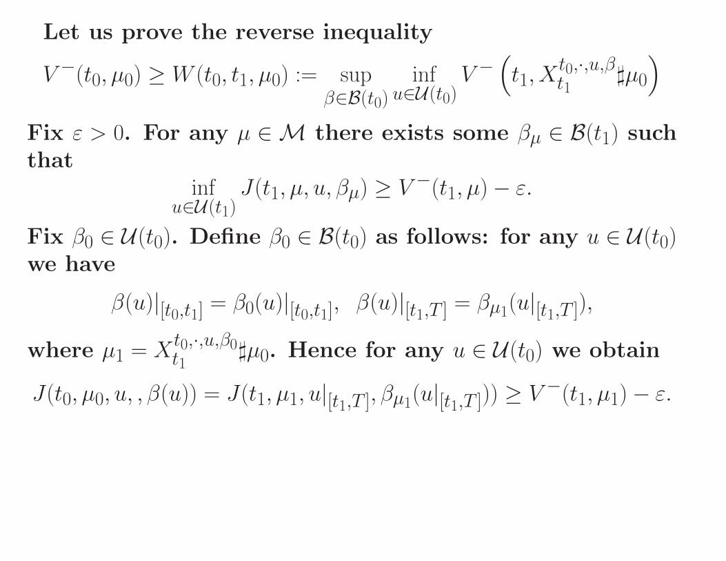
Let us prove the reverse inequality

V −(t0, µ0) ≥ W (t0, t1, µ0) := supβ∈B(t0)

infu∈U(t0)

V −(t1, X

t0,·,u,βt1

]µ0

)Fix ε > 0. For any µ ∈ M there exists some βµ ∈ B(t1) suchthat

infu∈U(t1)

J(t1, µ, u, βµ) ≥ V −(t1, µ)− ε.

Fix β0 ∈ U(t0). Define β0 ∈ B(t0) as follows: for any u ∈ U(t0)we have

β(u)|[t0,t1] = β0(u)|[t0,t1], β(u)|[t1,T ] = βµ1(u|[t1,T ]),

where µ1 = Xt0,·,u,β0t1

]µ0. Hence for any u ∈ U(t0) we obtain

J(t0, µ0, u, , β(u)) = J(t1, µ1, u|[t1,T ], βµ1(u|[t1,T ])) ≥ V −(t1, µ1)− ε.

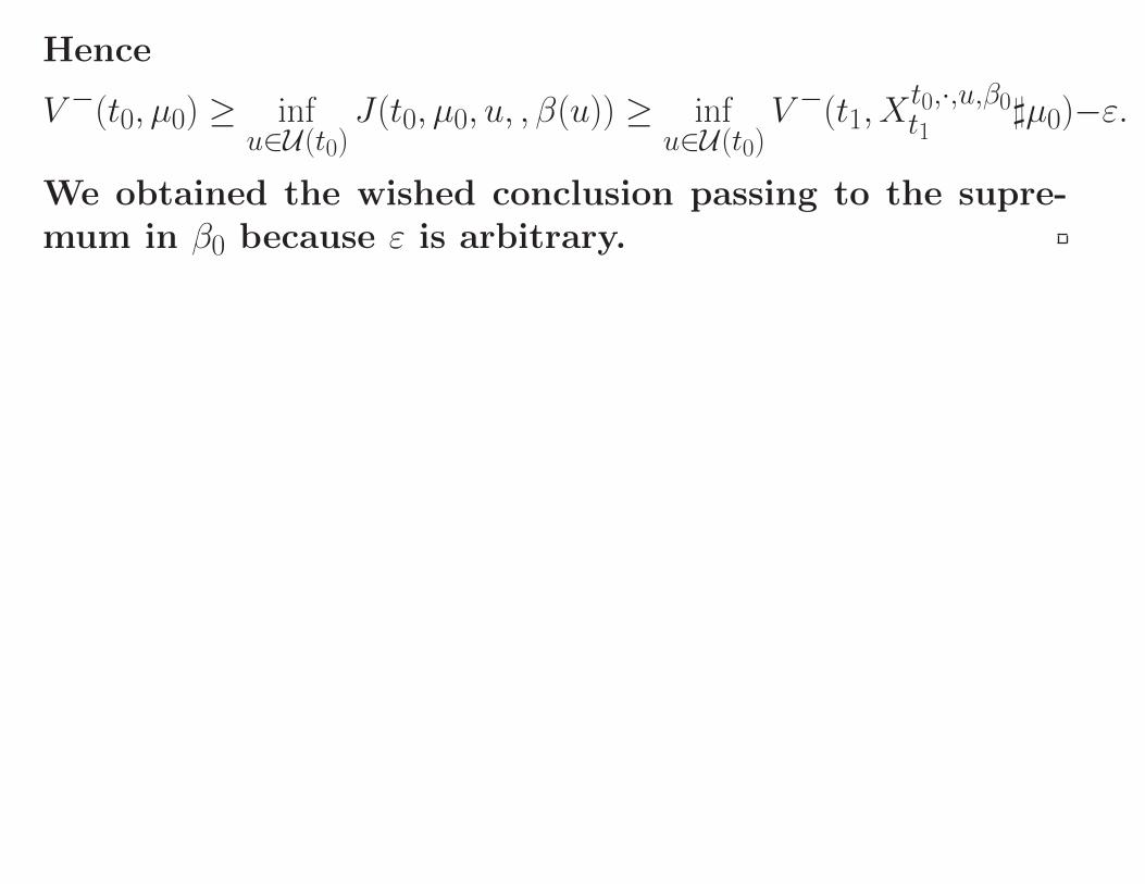
Hence

V −(t0, µ0) ≥ infu∈U(t0)

J(t0, µ0, u, , β(u)) ≥ infu∈U(t0)

V −(t1, Xt0,·,u,β0t1

]µ0)−ε.

We obtained the wished conclusion passing to the supre-mum in β0 because ε is arbitrary.

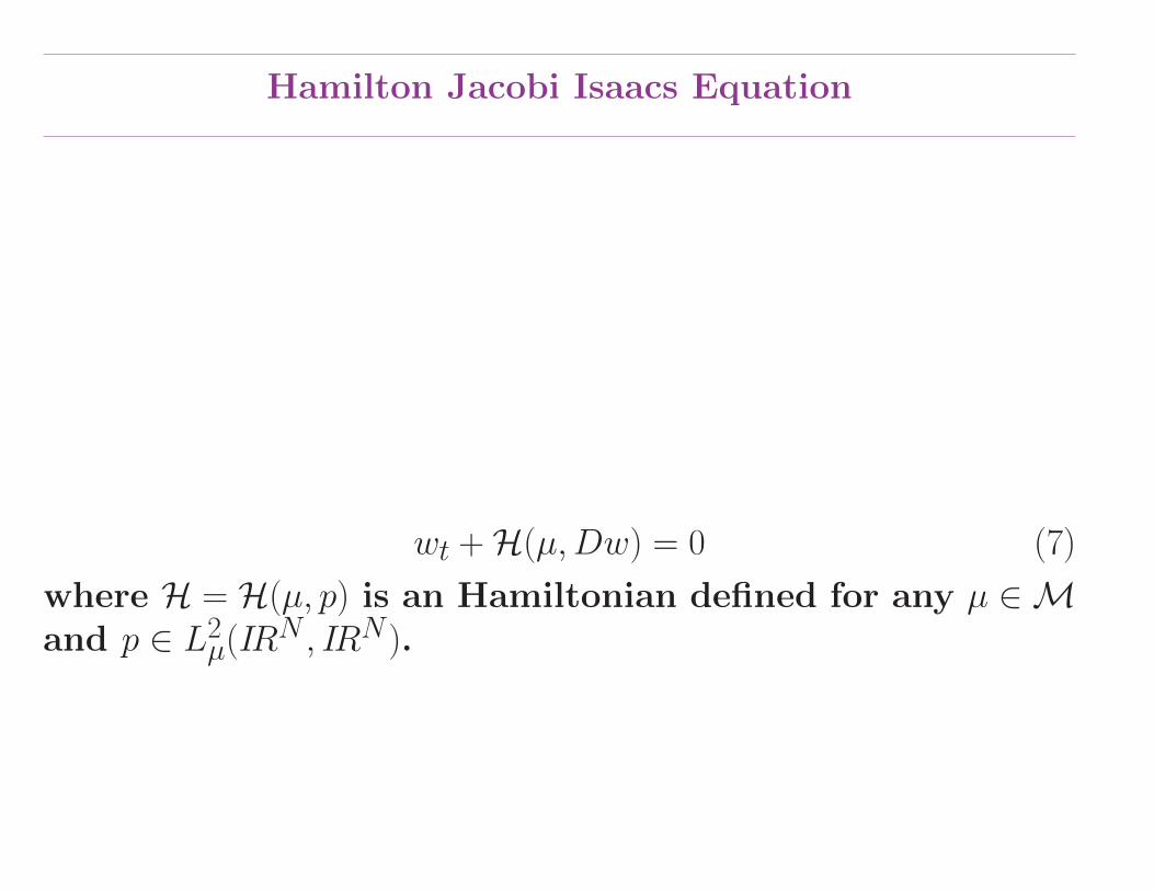
Hamilton Jacobi Isaacs Equation

wt +H(µ,Dw) = 0 (7)

where H = H(µ, p) is an Hamiltonian defined for any µ ∈Mand p ∈ L2

µ(IRN , IRN ).

Definition 7 (Sub- and super-differential) Let w : [0, T ]×M→IR be a function, (t0, µ0) ∈ (0, T )×M and let δ > 0. (pt, pµ) ∈IR×L2

µ(IRN , IRN ) belongs to the δ-super-differential D+δ w(t0, µ0)

to w at (t0, µ0) if, ∀ϕ ∈ Cb(IRN , IRN ),

lim sup‖ϕ‖

L2µ→0, t→t0

[w(t, (idIRN + ϕ)]µ0)− w(t0, µ0)− pt(t− t0)

−∫IRN

< ϕ(x), pµ(x) > dµ0(x)]1

‖ϕ‖L2µ

+ |t− t0|≤ δ

A pair (pt, pµ) ∈ IR × L2µ(IRN , IRN ) belongs to the δ-sub-

differential D−δ w(t0, µ0) to w at (t0, µ0) if (−pt,−pµ) belongsto the δ-super-differential to −w at (t0, µ0).

Solutions of Hamilton-Jacobi equation

Definition 8 We say that a map w : [0, T ] ×M → IR is asub-solution of the HJ equation (7) if w is upper semi-continuous and if, for any (t0, µ0) ∈ (0, T ) × M, for any(pt, pµ) ∈ D+

δ w(t0, µ0), we have for any δ > 0,

pt +H(µ0, pµ) ≥ −Cδ (8)

where C > 0 is a constant which depends only of H.

In a similar way, w is a super-solution of the HJ equa-tion (7) if w is lower semicontinuous and if, for any(t0, µ0) ∈ (0, T )×M, for any (pt, pµ) ∈ D−δ w(t0, µ0), we have

pt +H(µ0, pµ) ≤ Cδ . (9)

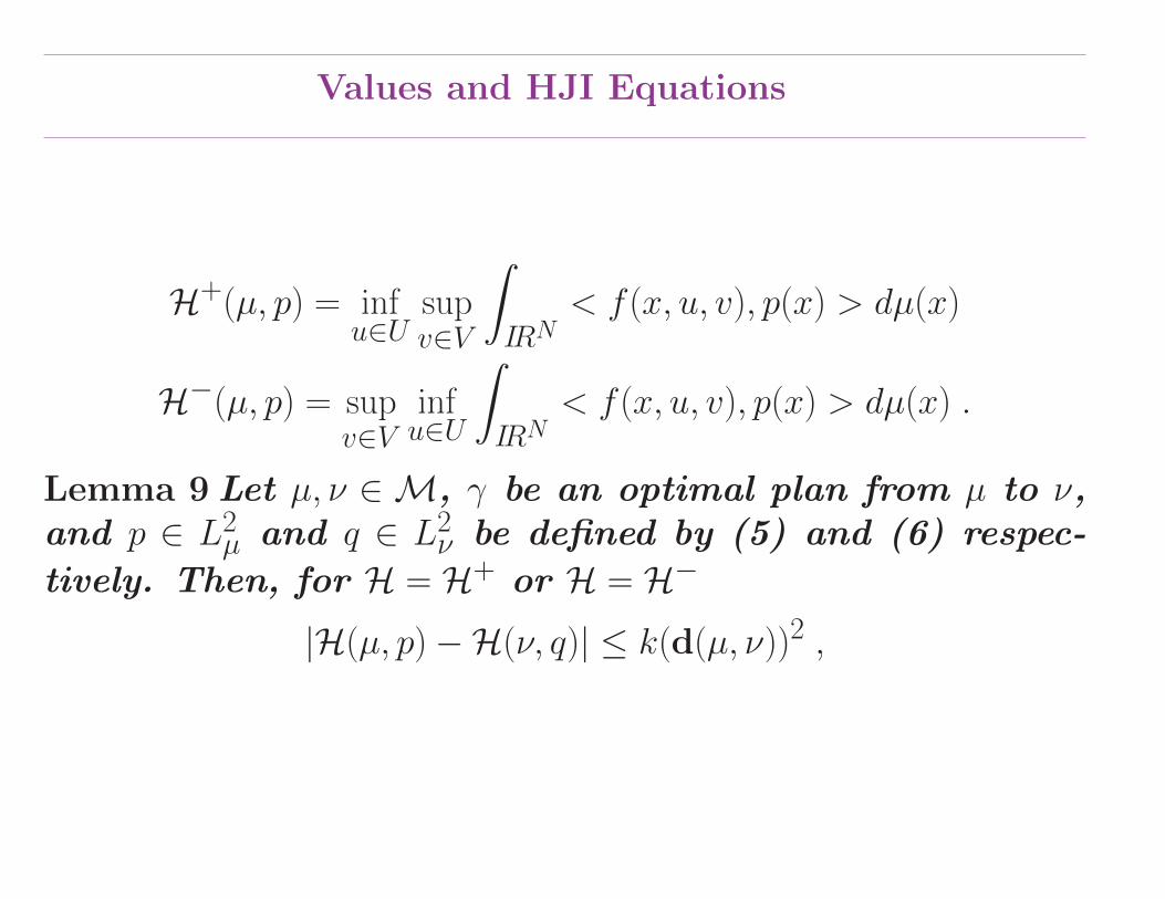
Values and HJI Equations

H+(µ, p) = infu∈U

supv∈V

∫IRN

< f (x, u, v), p(x) > dµ(x)

H−(µ, p) = supv∈V

infu∈U

∫IRN

< f (x, u, v), p(x) > dµ(x) .

Lemma 9 Let µ, ν ∈ M, γ be an optimal plan from µ to ν,and p ∈ L2

µ and q ∈ L2ν be defined by (5) and (6) respec-

tively. Then, for H = H+ or H = H−

|H(µ, p)−H(ν, q)| ≤ k(d(µ, ν))2 ,

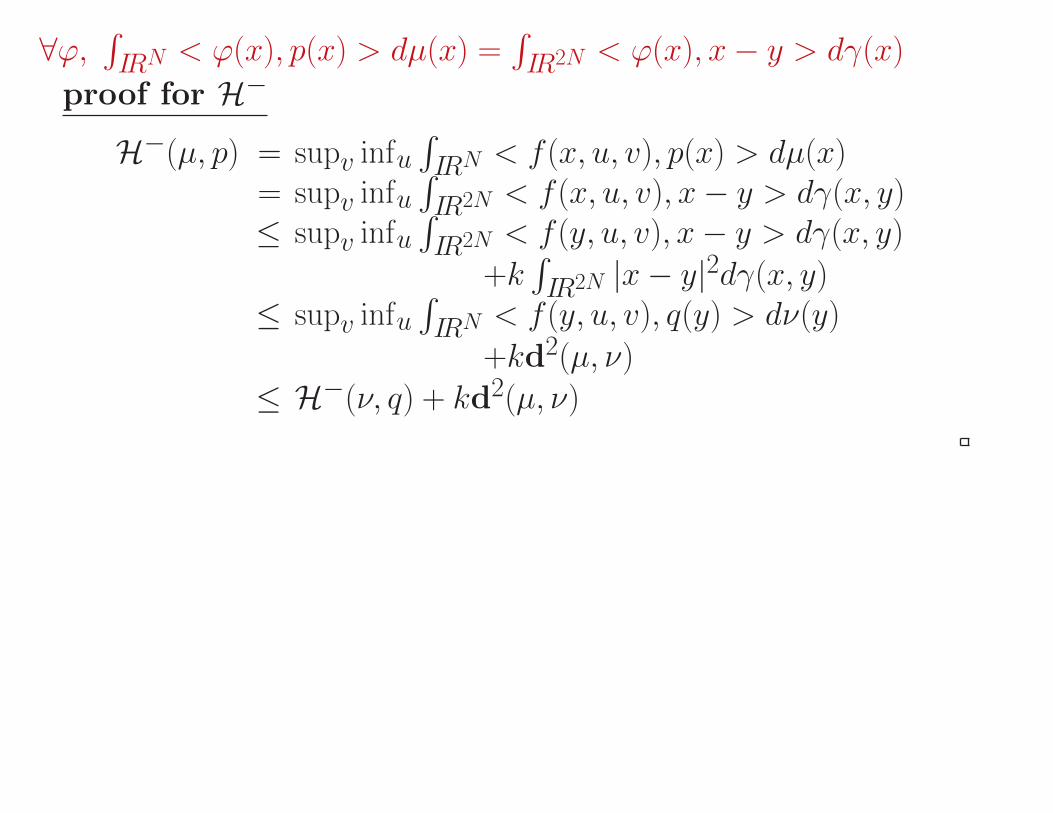
∀ϕ,∫IRN < ϕ(x), p(x) > dµ(x) =

∫IR2N < ϕ(x), x− y > dγ(x)

proof for H−

H−(µ, p) = supv infu∫IRN < f (x, u, v), p(x) > dµ(x)

= supv infu∫IR2N < f (x, u, v), x− y > dγ(x, y)

≤ supv infu∫IR2N < f (y, u, v), x− y > dγ(x, y)

+k∫IR2N |x− y|2dγ(x, y)

≤ supv infu∫IRN < f (y, u, v), q(y) > dν(y)

+kd2(µ, ν)

≤ H−(ν, q) + kd2(µ, ν)

Proposition 10 The upper value function V + is a solutionto HJI with H := H+ while the lower value function V − isa solution to HJI with H := H−.

proof of V + is a subsolution

Fix (t0, µ0) ∈ (0, T )×M, δ > 0 and (pt, pµ) ∈ D+δ V

+(t0, µ0).

We will prove that

pt +H(µ0, pµ) ≥ −δ (10)

Consider t ∈ (t0, T ). For any α ∈ A(t0) and β ∈ B(t0) defineϕα,β ∈ Cb(IRN , IRN ) such that

(idIRN + ϕα,β)(x) = Xt0,x,α,βt = x +

∫ t

t0

f (x(s), u(s), v(s))ds,

where (u, v) is associated with (α, β) and x(s) = Xt0,x,α,βs .

V +(t,Xt0,·,α,vt ]µ0) − V +(t0, µ0)− pt(t− t0)

−∫IRN

<

∫ t

t0

f (Xt0,x,α,βs , u(s), v(s))ds, pµ(x) > dµ(x)

≤ (‖ϕα,β‖L2µ

+ |t− t0|)(ε(t, ϕα,β) + δ)

(11)

where ε(t, ϕα,β)→ 0 as t→ t0 and ϕα,β → 0 in L2µ. Passing to

the sup on v and inf on α, we obtain by DDP

0 ≤ infα∈A(t0)

supv∈V(t0)

[

∫IRN

<

∫ t

t0

f (Xt0,x,α(v),vs , α(v)(s), v(s))ds, pµ(x) > dµ(x)

+pt(t− t0) + (‖ϕα(v),v‖L2µ

+ |t− t0|)(δ + ε(t, ϕα,β))]

for ‖ϕα(v),v‖L2µ

+ |t− t0| small enough.

For t close enough to t0 we obtain

0 ≤ infu∈U

supv∈V(t0)

[

∫IRN

<

∫ t

t0

f (x, u, v(s))ds, pµ(x) > dµ(x)

+pt(t− t0) + (‖ϕu,v‖L2µ

+ |t− t0|)(δ + ε(t, ϕu,v))]

when we restrict the infimum to nonanticipative strategiesα which has constant control values. Hence

0 ≤ infu∈U

supv∈V

[(t− t0)

∫IRN

< f (x, u, v)ds, pµ(x) > dµ(x)

+pt(t− t0) + (‖ϕu,v‖L2µ

+ |t− t0|)(δ + ε(t, ϕu,v))]

Dividing this inequality by t − t0 and letting t → t+0 gives,since ‖ϕu,v‖L2

µ= O(t− t0),

pt +H(µ0, pµ)) ≥ −(1 + M)δ .

Comparison Principle for HJI

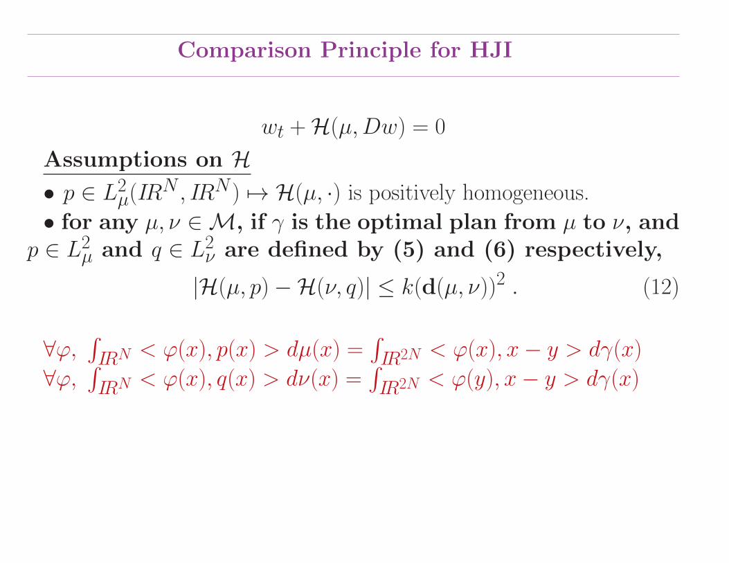
wt +H(µ,Dw) = 0

Assumptions on H• p ∈ L2

µ(IRN , IRN ) 7→ H(µ, ·) is positively homogeneous.

• for any µ, ν ∈M, if γ is the optimal plan from µ to ν, andp ∈ L2

µ and q ∈ L2ν are defined by (5) and (6) respectively,

|H(µ, p)−H(ν, q)| ≤ k(d(µ, ν))2 . (12)

∀ϕ,∫IRN < ϕ(x), p(x) > dµ(x) =

∫IR2N < ϕ(x), x− y > dγ(x)

∀ϕ,∫IRN < ϕ(x), q(x) > dν(x) =

∫IR2N < ϕ(y), x− y > dγ(x)

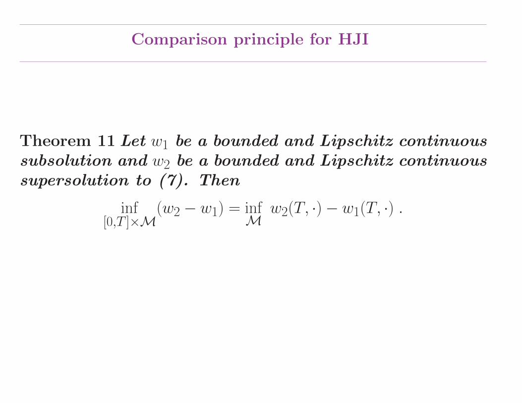
Comparison principle for HJI

Theorem 11 Let w1 be a bounded and Lipschitz continuoussubsolution and w2 be a bounded and Lipschitz continuoussupersolution to (7). Then

inf[0,T ]×M

(w2 − w1) = infM

w2(T, ·)− w1(T, ·) .

Proof of Comparison Principle

A = infµ∈M

w2(T, µ)− w1(T, µ) .

Since H is independant of w, w1−A is still a subsolution.So we suppose without loss of generality that A = 0.

By Contradiction

−ξ := infµ∈M, t∈[0,T ]

w2(t, µ)− w1(t, µ) < 0 .

And choose (t0, µ0) ∈ [0, T ]×M such that

(w2 − w1)(t0, µ0) < −ξ/2. (13)

Let C > 0 such that ∀δ > 0

∀(pt, pµ) ∈ D+δ w1(t0, µ0), pt +H(µ0, pµ) ≥ −Cδ

∀(pt, pµ) ∈ D−δ w2(t0, µ0) pt +H(µ0, pµ) ≤ Cδ .

Fixε > 0, η > 0 and δ > 0 sufficiently small such that

ξ > 2ηT +k2ε

2and 2Cδ + 2k(δ + k)2ε < η . (14)

We consider the following continuous function defined on([0, T ]×M)2:

Φ(s, µ, t, ν) = −w1(s, µ) + w2(t, ν) + 1ε

(d2(µ, ν) + (t− s)2

)− ηs .

Define

(µ, ν, s, t) ∈ Arg min[0,T ]×M

Φ

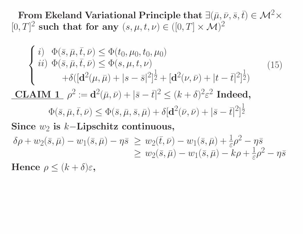
From Ekeland Variational Principle that ∃(µ, ν, s, t) ∈M2×[0, T ]2 such that for any (s, µ, t, ν) ∈ ([0, T ]×M)2

i) Φ(s, µ, t, ν) ≤ Φ(t0, µ0, t0, µ0)ii) Φ(s, µ, t, ν) ≤ Φ(s, µ, t, ν)

+δ([d2(µ, µ) + |s− s|2]12 + [d2(ν, ν) + |t− t|2]

12)

(15)

CLAIM 1 ρ2 := d2(µ, ν) + |s− t|2 ≤ (k + δ)2ε2 Indeed,

Φ(s, µ, t, ν) ≤ Φ(s, µ, s, µ) + δ[d2(ν, ν) + |s− t|2]12

Since w2 is k−Lipschitz continuous,

δρ + w2(s, µ)− w1(s, µ)− ηs ≥ w2(t, ν)− w1(s, µ) + 1ερ

2 − ηs≥ w2(s, µ)− w1(s, µ)− kρ + 1

ερ2 − ηs

Hence ρ ≤ (k + δ)ε,

Assume s, t ∈ (0, T ). Let γ be the optimal transport planbetween µ and ν and p ∈ L2(µ) and q ∈ L2(ν) associated.

CLAIM 2(2

ε(s− t)− η, 2

εp

)∈ D+

δ w1(s, µ),

(2

ε(s− t), 2

εq

)∈ D−δ w2(t, ν),

From (15)-ii), we have for any (s, µ),

Φ(s, µ, t, ν) ≤ Φ(s, µ, t, ν) + δ[d2(µ, µ) + |s− s|2]12.

w1(s, µ) ≤ w1(s, µ) + 1ε(d

2(µ, ν)− d2(µ, ν) + (s− t)2 − (s− t)2)

+δ[d2(µ, µ) + |s− s|2]12 + η(s− s)

(16)We will replace µ by (idIRN + ϕ)]µ with ϕ ∈ Cb(IRN , IRN )

Estimation

Observe γ′ = (idIRN + ϕ, idIRN)]γ is an admissible transportplan from (idIRN + ϕ)]µ to ν. Hence

d2((idIRN + ϕ)]µ, ν)− d2(µ, ν) ≤∫IR2N |x− y|2dγ′(x, y)−

∫IR2N |x− y|2dγ(x, y)

=∫IR2N (|x + ϕ(x)− y|2 − |x− y|2)dγ(x, y)

=∫IR2N (2 < x− y, ϕ(x) > +|ϕ(x)|2)dγ(x, y)

=∫IRN < 2p(x), ϕ(x) > dµ(x) + ‖ϕ‖2

L2µ

(from the def. of p)

w1(s, (idIRN + ϕ)]µ) ≤ w1(s, µ) + 1ε

∫IRN < 2p(x), ϕ(x) > dµ(x) + ‖ϕ‖2

L2µ)

+1ε(s− s)[(s− s) + 2(s− t)] + δ[d2(µ, µ) + |s− s|2]

12 + η(s− s)

So

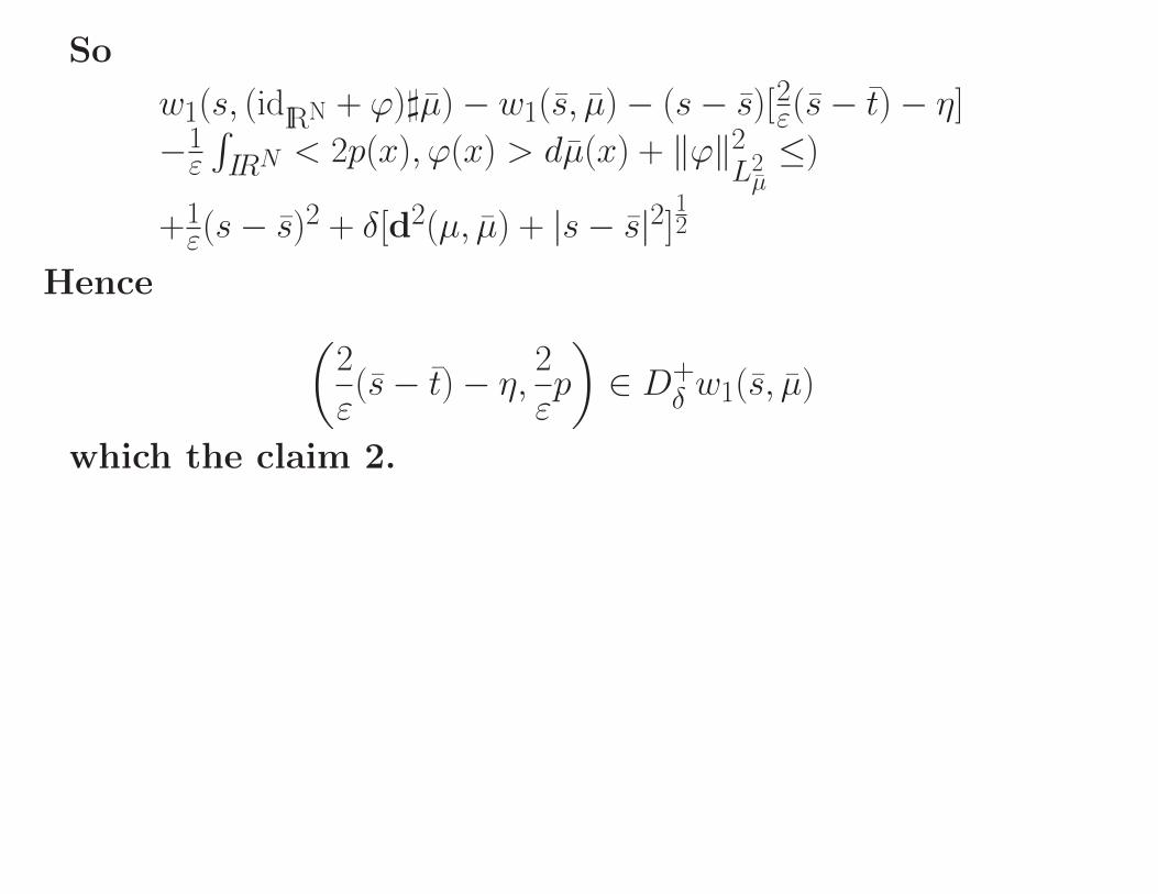
w1(s, (idIRN + ϕ)]µ)− w1(s, µ)− (s− s)[2ε(s− t)− η]

−1ε

∫IRN < 2p(x), ϕ(x) > dµ(x) + ‖ϕ‖2

L2µ≤)

+1ε(s− s)

2 + δ[d2(µ, µ) + |s− s|2]12

Hence (2

ε(s− t)− η, 2

εp

)∈ D+

δ w1(s, µ)

which the claim 2.

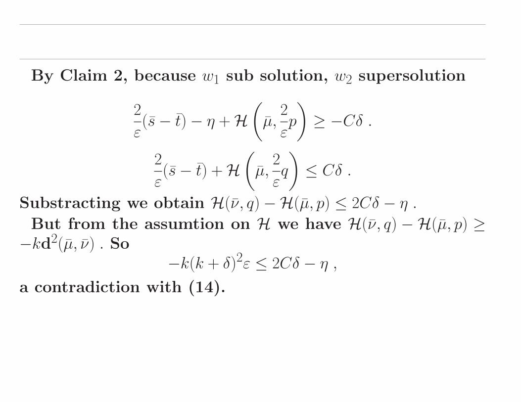
By Claim 2, because w1 sub solution, w2 supersolution

2

ε(s− t)− η +H

(µ,

2

εp

)≥ −Cδ .

2

ε(s− t) +H

(µ,

2

εq

)≤ Cδ .

Substracting we obtain H(ν, q)−H(µ, p) ≤ 2Cδ − η .But from the assumtion on H we have H(ν, q) −H(µ, p) ≥−kd2(µ, ν) . So

−k(k + δ)2ε ≤ 2Cδ − η ,a contradiction with (14).

We have to check that s and t cannot be equal to 0 or T .Let us assume for instance that s = T . We first note that

Φ(t0, µ0, t0, µ0) = w2(t0, µ0)− w1(t0, µ0)− ηt0 ≤ −ξ/2

From (Ekeland), i), we have

Φ(s, µ, t, ν) ≤ Φ(t0, µ0, t0, µ0) ≤ −ξ/2 .

Since s = T and w2 is k−Lipschitz continuous, we get (set-

ting as before ρ := [d2(ν, ν) + |s− t|2]12)

−ξ/2 ≥ w2(t, ν)− w1(T, µ) + 1ερ

2 − ηT≥ w2(T, µ)− w1(T, µ)− kρ + 1

ερ2 − ηT

≥ −kρ + 1ερ

2 − ηT ,

A contradiction with the choices of η, δ, ε and the estima-tion of ρ.

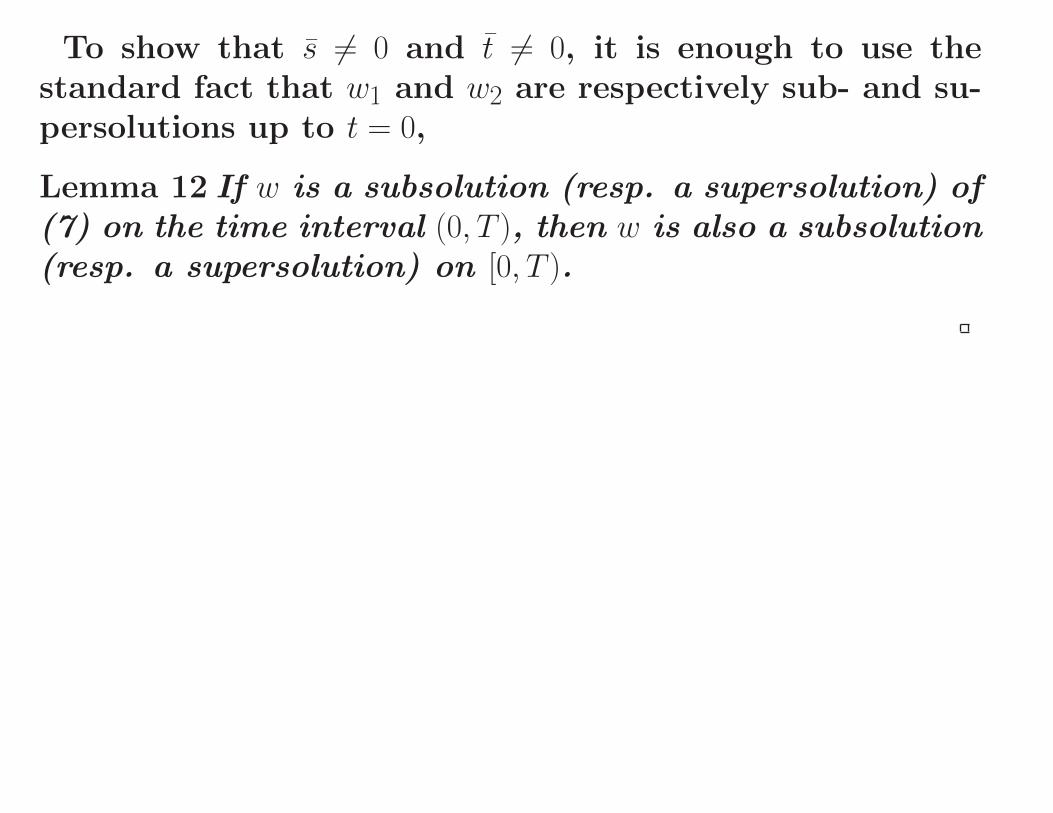
To show that s 6= 0 and t 6= 0, it is enough to use thestandard fact that w1 and w2 are respectively sub- and su-persolutions up to t = 0,

Lemma 12 If w is a subsolution (resp. a supersolution) of(7) on the time interval (0, T ), then w is also a subsolution(resp. a supersolution) on [0, T ).

Uniqueness Result for HJI

Corollary 13 There exists at most one lipschitz continuoussolution of (7) satisfying

w(T, µ) =

∫IRN

g(x)dµ(x) ,∀µ ∈M.

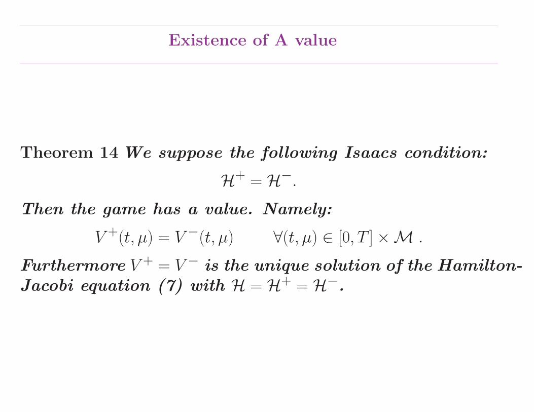
Existence of A value

Theorem 14 We suppose the following Isaacs condition:

H+ = H−.Then the game has a value. Namely:

V +(t, µ) = V −(t, µ) ∀(t, µ) ∈ [0, T ]×M .

Furthermore V + = V − is the unique solution of the Hamilton-Jacobi equation (7) with H = H+ = H−.

Thank You for your Attention