Tutorial Intro. to Modern Formal Methods: Mechanized ... · Some Different Approaches to Formal...
161
Tutorial Intro. to Modern Formal Methods: Mechanized Formal Analysis Using Model Checking, Theorem Proving SMT Solving, Abstraction, and Static Analysis With SAL, PVS, and Yices, and more John Rushby Computer Science Laboratory SRI International Menlo Park CA USA John Rushby Formal Calculation: 1
Transcript of Tutorial Intro. to Modern Formal Methods: Mechanized ... · Some Different Approaches to Formal...

Tutorial Intro. to Modern Formal Methods:
Mechanized Formal Analysis
Using Model Checking, Theorem Proving
SMT Solving, Abstraction, and Static Analysis
With SAL, PVS, and Yices, and more
John Rushby
Computer Science Laboratory
SRI International
Menlo Park CA USA
John Rushby Formal Calculation: 1

Some Different Approaches to Formal Analysis
(of safety properties of concurrent systems
defined as transition relations)
. . . to be demonstrated on a concrete example
Namely, Lamport’s Bakery Algorithm
• Explicit, symbolic, bounded model checking
• Deduction (theorem proving)
• Abstraction and model checking
• Automated abstraction (failure tolerant theorem proving)
• Bounded model checking (for infinite state systems)
Focus is on pragmatics and tools (many demos), not theory
If there is time and interest, will also look at test generation,
static analysis, and timed systems
John Rushby Formal Calculation: 2
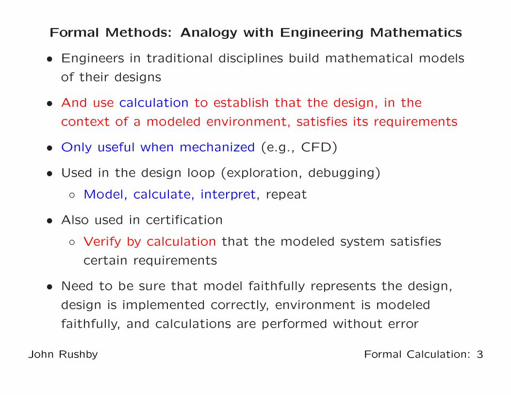
Formal Methods: Analogy with Engineering Mathematics
• Engineers in traditional disciplines build mathematical models
of their designs
• And use calculation to establish that the design, in the
context of a modeled environment, satisfies its requirements
• Only useful when mechanized (e.g., CFD)
• Used in the design loop (exploration, debugging)
◦ Model, calculate, interpret, repeat
• Also used in certification
◦ Verify by calculation that the modeled system satisfies
certain requirements
• Need to be sure that model faithfully represents the design,
design is implemented correctly, environment is modeled
faithfully, and calculations are performed without error
John Rushby Formal Calculation: 3
Formal Methods: Analogy with Engineering Math (ctd.)
• Formal methods: same idea, applied to computational
systems
• The applied math of Computer Science is formal logic
• So the models are formal descriptions in some logical system
◦ E.g., a program reinterpreted as a mathematical formula
rather than instructions to a machine
• And calculation is mechanized by automated deduction:
theorem proving, model checking, static analysis, etc.
• Formal calculations (can) cover all modeled behaviors
• If the model is accurate, this provides verification
• If the model is approximate, can still be good for debugging
(aka. refutation)
John Rushby Formal Calculation: 4
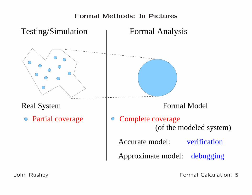
Formal Methods: In Pictures
Testing/Simulation Formal Analysis
Complete coverage
Formal ModelReal System
Partial coverage(of the modeled system)
Accurate model:
Approximate model:
verification
debugging
John Rushby Formal Calculation: 5
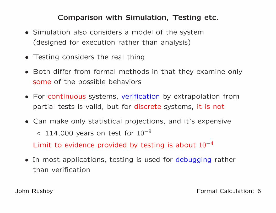
Comparison with Simulation, Testing etc.
• Simulation also considers a model of the system
(designed for execution rather than analysis)
• Testing considers the real thing
• Both differ from formal methods in that they examine only
some of the possible behaviors
• For continuous systems, verification by extrapolation from
partial tests is valid, but for discrete systems, it is not
• Can make only statistical projections, and it’s expensive
◦ 114,000 years on test for 10−9
Limit to evidence provided by testing is about 10−4
• In most applications, testing is used for debugging rather
than verification
John Rushby Formal Calculation: 6
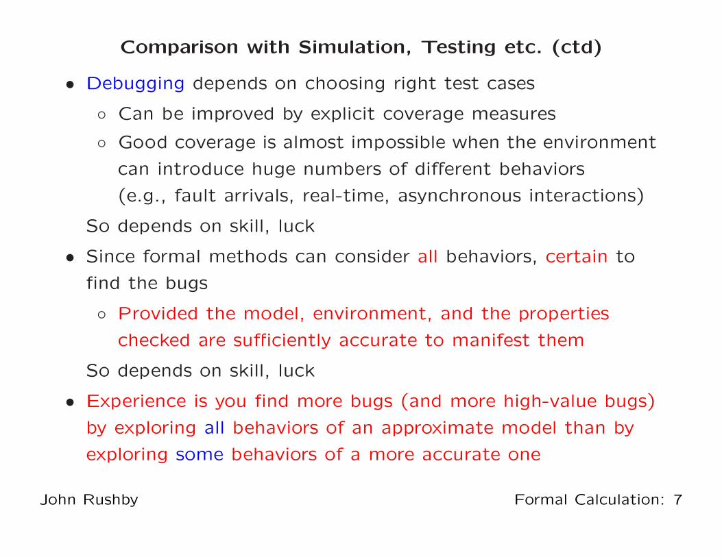
Comparison with Simulation, Testing etc. (ctd)
• Debugging depends on choosing right test cases
◦ Can be improved by explicit coverage measures
◦ Good coverage is almost impossible when the environment
can introduce huge numbers of different behaviors
(e.g., fault arrivals, real-time, asynchronous interactions)
So depends on skill, luck
• Since formal methods can consider all behaviors, certain to
find the bugs
◦ Provided the model, environment, and the properties
checked are sufficiently accurate to manifest them
So depends on skill, luck
• Experience is you find more bugs (and more high-value bugs)
by exploring all behaviors of an approximate model than by
exploring some behaviors of a more accurate one
John Rushby Formal Calculation: 7
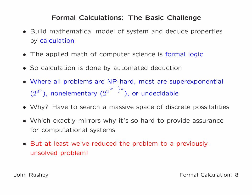
Formal Calculations: The Basic Challenge
• Build mathematical model of system and deduce properties
by calculation
• The applied math of computer science is formal logic
• So calculation is done by automated deduction
• Where all problems are NP-hard, most are superexponential
(22n
), nonelementary (222
...
}n
), or undecidable
• Why? Have to search a massive space of discrete possibilities
• Which exactly mirrors why it’s so hard to provide assurance
for computational systems
• But at least we’ve reduced the problem to a previously
unsolved problem!
John Rushby Formal Calculation: 8

Formal Calculations: Meeting The Basic Challenge
Ways to cope with the massive computational complexity
• Use human guidance
◦ That’s interactive theorem proving—e.g., PVS
• Restrict attention to specific kinds of problems
◦ E.g., model checking—focuses on state machines etc.
• Use approximate models, incomplete search
◦ model checkers are often used this way
• Aim at something other than verification
◦ E.g., bug finding, test case generation
• Verify weak properties
◦ That’s what static analysis typically does
• Give up soundness and/or completeness
◦ Again, that’s what static analysis typically does
John Rushby Formal Calculation: 9

Let’s do an example: Bakery
John Rushby Formal Calculation: 10
The Bakery Algorithm for Distributed Mutual Exclusion
• Idea is based on the way people queue for service in US
delicatessens and bakeries (or Vietnam Airlines in HCMC)
• A machine dispenses tickets printed with numbers that
increase monotonically
• People who want service take a ticket
• The unserved person with the lowest numbered ticket is
served next
◦ Safe: at most one person is served
(i.e., is in the “critical section”) at a time
◦ Live: each person is eventually served
• Preserve the idea without centralized ticket dispenser
John Rushby Formal Calculation: 11

Informal Protocol Description
• Works for n ≥ 1 processes
• Each process has a ticket register, initially zero
• When it wants to enter its critical section, a process sets its
ticket greater than that of any other process
• Then it waits until its ticket is smaller than that of any other
process with a nonzero ticket
• At which point it enters its critical section
• Resets its ticket to zero when it exits its critical section
• Show that at most one process is in its critical section at any
time (i.e., mutual exclusion)
John Rushby Formal Calculation: 12
Formal Modeling and Analysis
• Build a mathematical model of the protocol
• Analyze it for a desired property
• Must choose how much detail to include in the model
◦ Too much detail: analysis may be infeasible
◦ Too little detail: analysis may be inaccurate
(i.e., fail to detect bugs, or report spurious ones)
◦ Must also choose a modeling style that supports intended
form of analysis
• Requires judgment (skill, luck) to do this
John Rushby Formal Calculation: 13

Modeling the Example System and its Properties:
Accuracy and Level of Detail
• The protocol uses shared memory and is sensitive to the
atomicity of concurrent reads and writes
• And to the memory model (on multiprocessors with relaxed
memory models, reads and writes from different processors
may be reordered)
• And to any faults the memory may exhibit
• If we wish to examine the mutual exclusion property of a
particular implementation of the protocol, we will need to
represent the memory model, fault model, and atomicity
employed—which will be quite challenging
• Abstractly (or at first), we may prefer to focus on the
behavior of the protocol in an ideal environment with
fault-free sequentially consistent atomic memory
John Rushby Formal Calculation: 14
Modeling the Example System and its Properties (ctd.)
• Also, although the protocol is suitable for n processes, we
may prefer to focus on the important special case n = 2
• And although each process will perform activities other than
the given protocol, we will abstract these details away and
assume each process is in one of three phases
idle: performing work outside its critical section
trying: to enter its critical section
critical: performing work inside its critical section
John Rushby Formal Calculation: 15
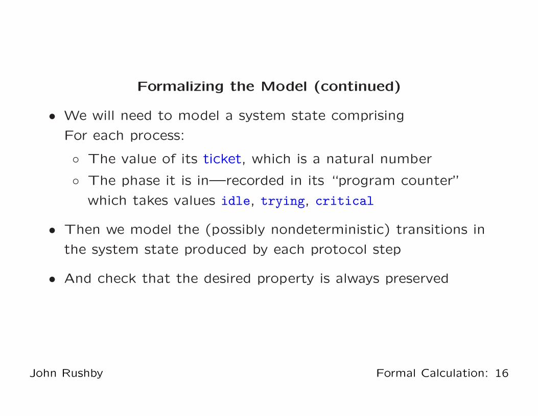
Formalizing the Model (continued)
• We will need to model a system state comprising
For each process:
◦ The value of its ticket, which is a natural number
◦ The phase it is in—recorded in its “program counter”
which takes values idle, trying, critical
• Then we model the (possibly nondeterministic) transitions in
the system state produced by each protocol step
• And check that the desired property is always preserved
John Rushby Formal Calculation: 16
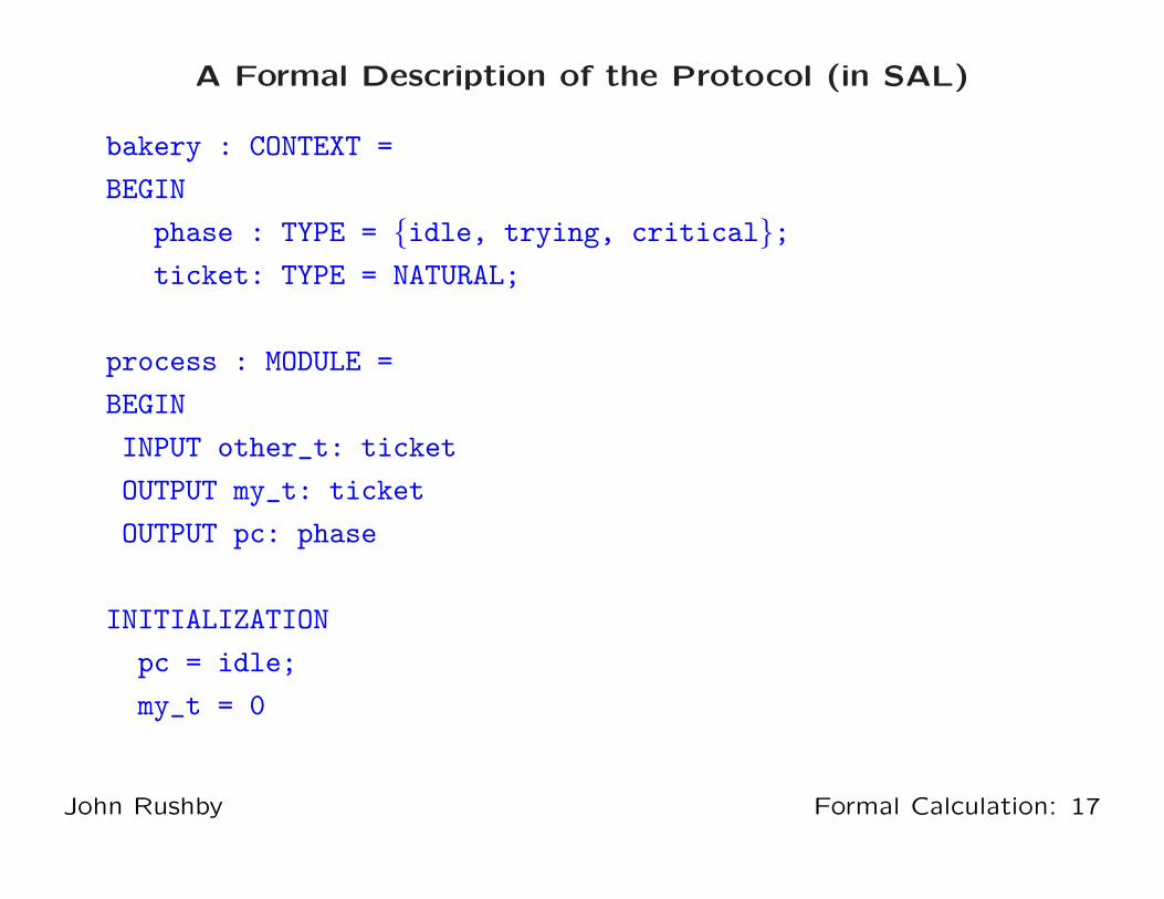
A Formal Description of the Protocol (in SAL)
bakery : CONTEXT =
BEGIN
phase : TYPE = {idle, trying, critical};
ticket: TYPE = NATURAL;
process : MODULE =
BEGIN
INPUT other_t: ticket
OUTPUT my_t: ticket
OUTPUT pc: phase
INITIALIZATION
pc = idle;
my_t = 0
John Rushby Formal Calculation: 17
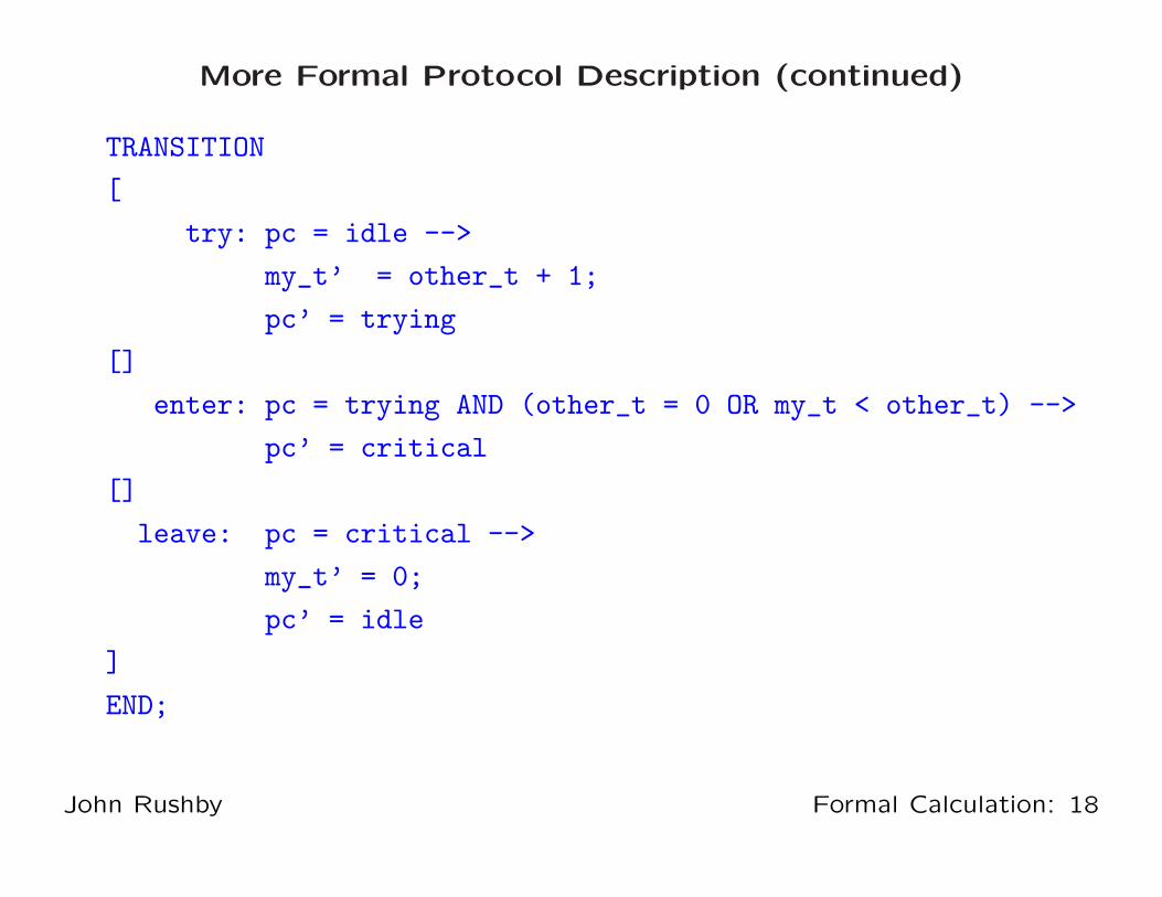
More Formal Protocol Description (continued)
TRANSITION
[
try: pc = idle -->
my_t’ = other_t + 1;
pc’ = trying
[]
enter: pc = trying AND (other_t = 0 OR my_t < other_t) -->
pc’ = critical
[]
leave: pc = critical -->
my_t’ = 0;
pc’ = idle
]
END;
John Rushby Formal Calculation: 18

More Formal Protocol Description (continued again)
P1 : MODULE = RENAME pc TO pc1 IN process;
P2 : MODULE = RENAME other_t TO my_t,
my_t TO other_t,
pc TO pc2 IN process;
system : MODULE = P1 [] P2;
safety: THEOREM
system |- G(NOT (pc1 = critical AND pc2 = critical));
END
John Rushby Formal Calculation: 19

Analyzing the Specification Using Model Checking
• They are called model checkers because they check whether
a system, interpreted as an automaton, is a (Kripke) model
of a property expressed as a temporal logic formula
• The simplest type of model checker is one that does explicit
state exploration
◦ Basically, a simulator that remembers the states it’s seen
before and backtracks to explore all of them (either
depth-first, breadth-first, or a combination)
◦ Defeated by the state explosion problem at around a few
tens of millions of states
• To get further, need symbolic representations (a short
formula can represent many explicit states)
◦ Symbolic model checkers use BDDs
◦ Bounded model checkers use SAT and SMT solvers
John Rushby Formal Calculation: 20
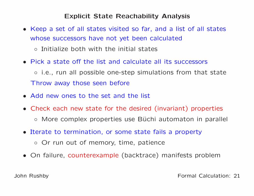
Explicit State Reachability Analysis
• Keep a set of all states visited so far, and a list of all states
whose successors have not yet been calculated
◦ Initialize both with the initial states
• Pick a state off the list and calculate all its successors
◦ i.e., run all possible one-step simulations from that state
Throw away those seen before
• Add new ones to the set and the list
• Check each new state for the desired (invariant) properties
◦ More complex properties use Buchi automaton in parallel
• Iterate to termination, or some state fails a property
◦ Or run out of memory, time, patience
• On failure, counterexample (backtrace) manifests problem
John Rushby Formal Calculation: 21
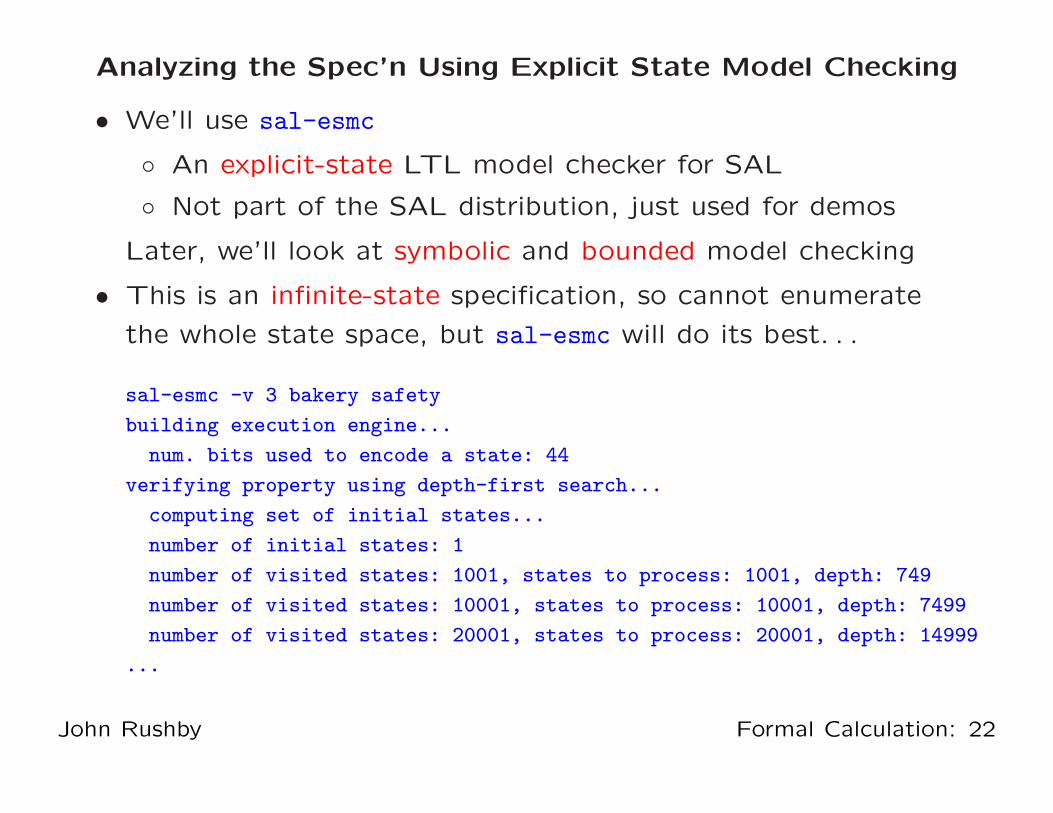
Analyzing the Spec’n Using Explicit State Model Checking
• We’ll use sal-esmc
◦ An explicit-state LTL model checker for SAL
◦ Not part of the SAL distribution, just used for demos
Later, we’ll look at symbolic and bounded model checking
• This is an infinite-state specification, so cannot enumerate
the whole state space, but sal-esmc will do its best. . .
sal-esmc -v 3 bakery safety
building execution engine...
num. bits used to encode a state: 44
verifying property using depth-first search...
computing set of initial states...
number of initial states: 1
number of visited states: 1001, states to process: 1001, depth: 749
number of visited states: 10001, states to process: 10001, depth: 7499
number of visited states: 20001, states to process: 20001, depth: 14999
...
John Rushby Formal Calculation: 22
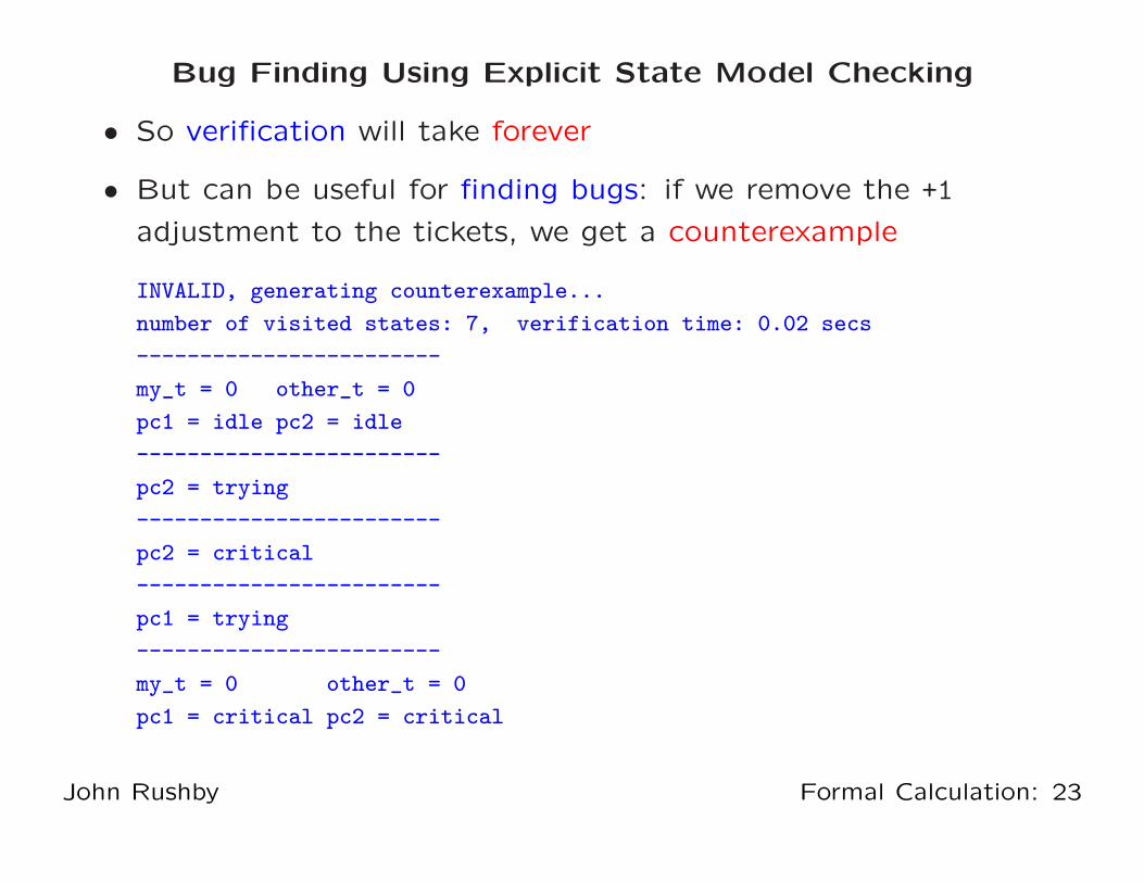
Bug Finding Using Explicit State Model Checking
• So verification will take forever
• But can be useful for finding bugs: if we remove the +1
adjustment to the tickets, we get a counterexample
INVALID, generating counterexample...
number of visited states: 7, verification time: 0.02 secs
------------------------
my_t = 0 other_t = 0
pc1 = idle pc2 = idle
------------------------
pc2 = trying
------------------------
pc2 = critical
------------------------
pc1 = trying
------------------------
my_t = 0 other_t = 0
pc1 = critical pc2 = critical
John Rushby Formal Calculation: 23
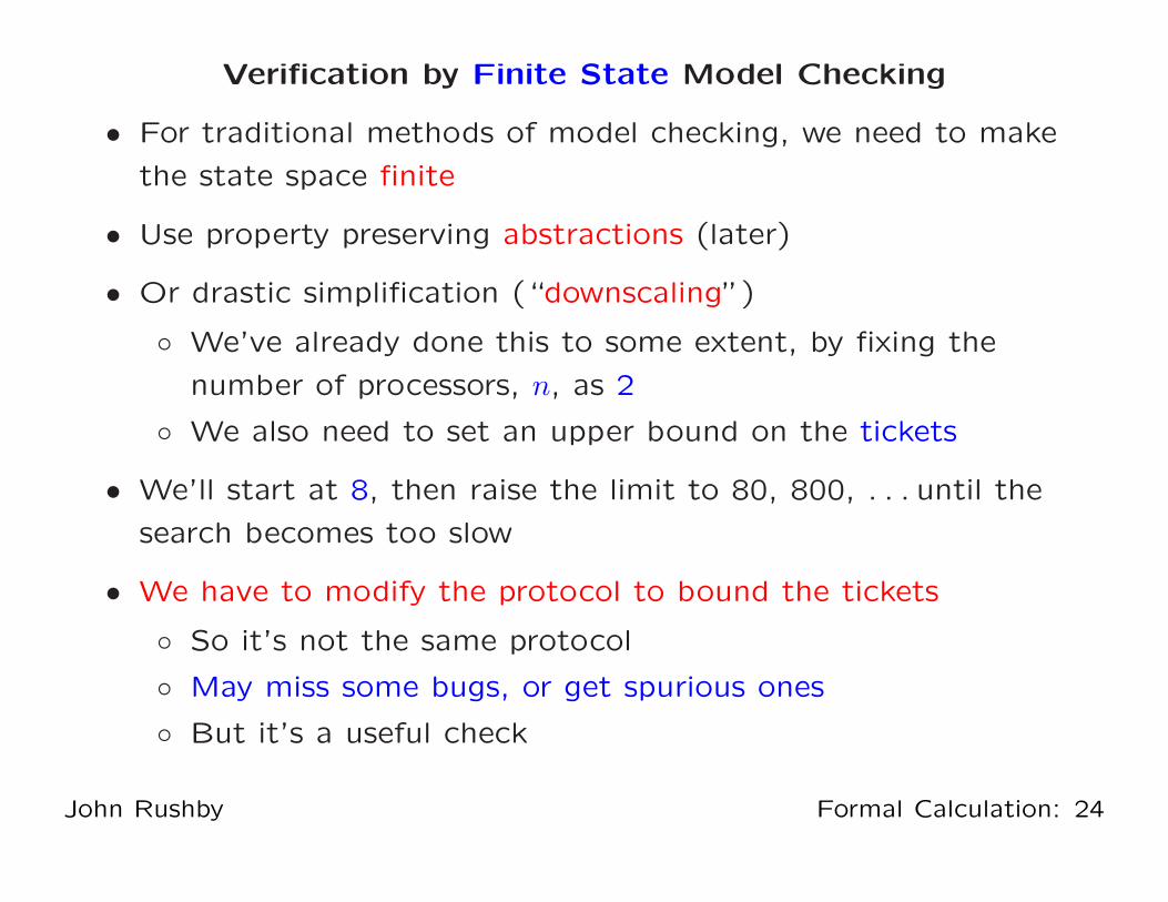
Verification by Finite State Model Checking
• For traditional methods of model checking, we need to make
the state space finite
• Use property preserving abstractions (later)
• Or drastic simplification (“downscaling”)
◦ We’ve already done this to some extent, by fixing the
number of processors, n, as 2
◦ We also need to set an upper bound on the tickets
• We’ll start at 8, then raise the limit to 80, 800, . . . until the
search becomes too slow
• We have to modify the protocol to bound the tickets
◦ So it’s not the same protocol
◦ May miss some bugs, or get spurious ones
◦ But it’s a useful check
John Rushby Formal Calculation: 24

The Bounded Specification in SAL
bakery : CONTEXT =
BEGIN
phase : TYPE = {idle, trying, critical};
max: NATURAL = 8;
ticket: TYPE = [0..max];
process : MODULE =
BEGIN
INPUT other_t: ticket
OUTPUT my_t: ticket
OUTPUT pc: phase
INITIALIZATION
pc = idle;
my_t = 0
John Rushby Formal Calculation: 25
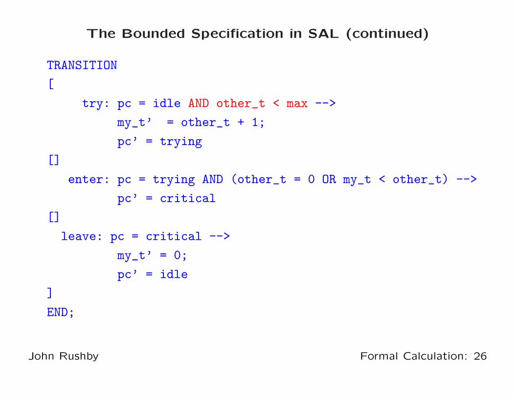
The Bounded Specification in SAL (continued)
TRANSITION
[
try: pc = idle AND other_t < max -->
my_t’ = other_t + 1;
pc’ = trying
[]
enter: pc = trying AND (other_t = 0 OR my_t < other_t) -->
pc’ = critical
[]
leave: pc = critical -->
my_t’ = 0;
pc’ = idle
]
END;
John Rushby Formal Calculation: 26

The Bounded Specification in SAL (continued again)
P1 : MODULE = RENAME pc TO pc1 IN process;
P2 : MODULE = RENAME other_t TO my_t,
my_t TO other_t,
pc TO pc2 IN process;
system : MODULE = P1 [] P2;
safety: THEOREM
system |- G(NOT (pc1 = critical AND pc2 = critical));
END
John Rushby Formal Calculation: 27

Results of Model Checking
• For max = 800, sal-esmc reports
sal-esmc -v 3 smallbakery safety
num. bits used to encode a state: 24
verifying property using depth-first search...
computing set of initial states...
number of initial states: 1
number of visited states: 1001, states to process: 1001, depth: 749
number of visited states: 2001, states to process: 2001, depth: 1499
number of visited states: 3001, states to process: 3001, depth: 2249
number of visited states: 4002, states to process: 804, depth: 602
number of visited states: 5002, states to process: 1804, depth: 1352
number of visited states: 6002, states to process: 2804, depth: 2102
number of visited states: 6397
verification time: 0.54 secs
proved.
• For max = 8000, number of visited states grows to 63,997,
and time to 23.86 secs
John Rushby Formal Calculation: 28
More Explicit State Checks
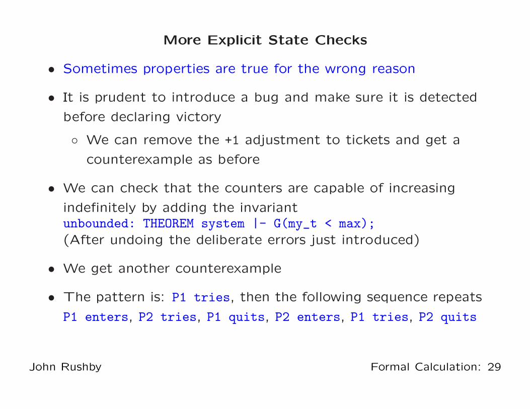
• Sometimes properties are true for the wrong reason
• It is prudent to introduce a bug and make sure it is detected
before declaring victory
◦ We can remove the +1 adjustment to tickets and get a
counterexample as before
• We can check that the counters are capable of increasing
indefinitely by adding the invariantunbounded: THEOREM system |- G(my_t < max);
(After undoing the deliberate errors just introduced)
• We get another counterexample
• The pattern is: P1 tries, then the following sequence repeats
P1 enters, P2 tries, P1 quits, P2 enters, P1 tries, P2 quits
John Rushby Formal Calculation: 29

Benefits of Explicit State Model Checking
• Can only explore a few million states, but that’s enough
when there are plenty of bugs to find
• Can use hashing (supertrace) to go further
• Can have arbitrarily complex transition relation
◦ Language can include any datatypes and operations
supported by the API
• Breadth first search finds short counterexamples
◦ Can write special search strategies to target specific
cases, or to ignore others (symmetry, partial order)
• LTL is handled via Buchi automata
• Can evaluate functions, not just predicates, on the reachable
states: can calculate worst-cases, do optimization
But it runs out of steam on big examples
John Rushby Formal Calculation: 30
Analysis by Symbolic Model Checking (SMC)
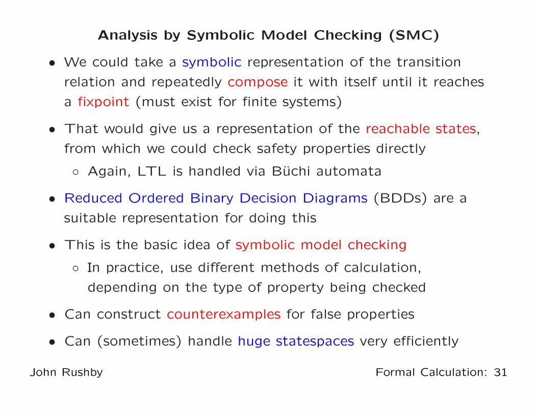
• We could take a symbolic representation of the transition
relation and repeatedly compose it with itself until it reaches
a fixpoint (must exist for finite systems)
• That would give us a representation of the reachable states,
from which we could check safety properties directly
◦ Again, LTL is handled via Buchi automata
• Reduced Ordered Binary Decision Diagrams (BDDs) are a
suitable representation for doing this
• This is the basic idea of symbolic model checking
◦ In practice, use different methods of calculation,
depending on the type of property being checked
• Can construct counterexamples for false properties
• Can (sometimes) handle huge statespaces very efficiently
John Rushby Formal Calculation: 31

Symbolic Model Checking (ctd)
• Our symbolic representation is a purely Boolean one
• So we have to compile the transition relation down to what
is essentially a circuit
◦ Bounded integers represented by bitvectors of suitable size
◦ Addition requires the circuit for a boolean adder
◦ Similarly for other datatypes and operations
• We are doing a kind of circuit synthesis
• May fail for large or complex transition relations
• BDD operations depend on finding a good variable ordering
• Automated heuristics usually effective to about 600 state bits
• After that, manual ordering, special tricks are needed
• Seldom get beyond 1,000 state bits
John Rushby Formal Calculation: 32
Symbolic Model Checking with SAL
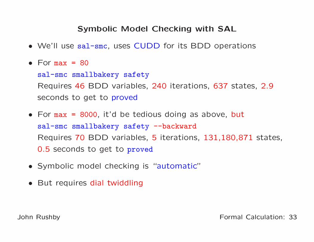
• We’ll use sal-smc, uses CUDD for its BDD operations
• For max = 80
sal-smc smallbakery safety
Requires 46 BDD variables, 240 iterations, 637 states, 2.9
seconds to get to proved
• For max = 8000, it’d be tedious doing as above, but
sal-smc smallbakery safety --backward
Requires 70 BDD variables, 5 iterations, 131,180,871 states,
0.5 seconds to get to proved
• Symbolic model checking is “automatic”
• But requires dial twiddling
John Rushby Formal Calculation: 33

More Checks With Symbolic Model Checking
• Do the tickets always increase without bound?bounded: LEMMA system |- F(my_t > 3);
• The counterexample to this liveness property is a prefix,
followed by a loop (lasso)
• The pattern is P1 tries, enters, leaves, and then repeats
• Does P1 ever get into the critical region?liveness: THEOREM system |- F(pc1 = critical);
Same counterexample as above (with P2 rather than P1)
• If it tries, does it always succeed?response: THEOREM system |-
G(pc1 = trying => F(pc1 = critical));
Proved
John Rushby Formal Calculation: 34
Yet More Checks With Symbolic Model Checking
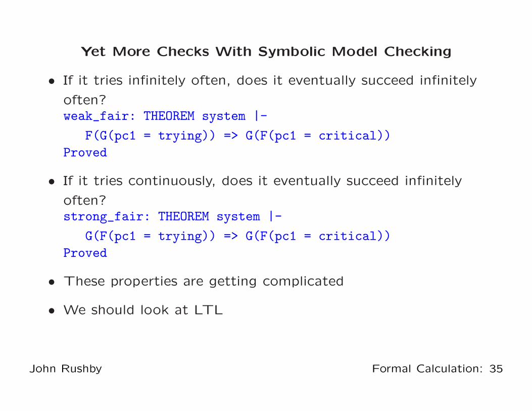
• If it tries infinitely often, does it eventually succeed infinitely
often?weak_fair: THEOREM system |-
F(G(pc1 = trying)) => G(F(pc1 = critical))
Proved
• If it tries continuously, does it eventually succeed infinitely
often?strong_fair: THEOREM system |-
G(F(pc1 = trying)) => G(F(pc1 = critical))
Proved
• These properties are getting complicated
• We should look at LTL
John Rushby Formal Calculation: 35
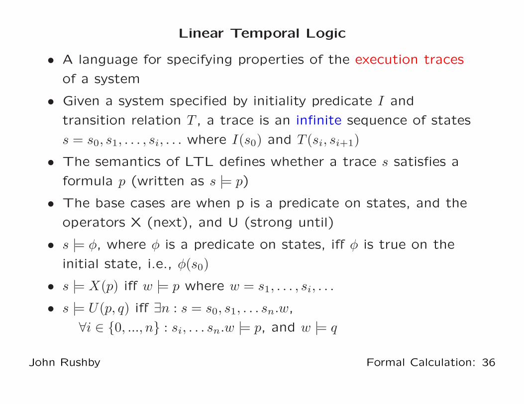
Linear Temporal Logic
• A language for specifying properties of the execution traces
of a system
• Given a system specified by initiality predicate I and
transition relation T , a trace is an infinite sequence of states
s = s0, s1, . . . , si, . . . where I(s0) and T (si, si+1)
• The semantics of LTL defines whether a trace s satisfies a
formula p (written as s |= p)
• The base cases are when p is a predicate on states, and the
operators X (next), and U (strong until)
• s |= φ, where φ is a predicate on states, iff φ is true on the
initial state, i.e., φ(s0)
• s |= X(p) iff w |= p where w = s1, . . . , si, . . .
• s |= U(p, q) iff ∃n : s = s0, s1, . . . sn.w,
∀i ∈ {0, ..., n} : si, . . . sn.w |= p, and w |= q
John Rushby Formal Calculation: 36
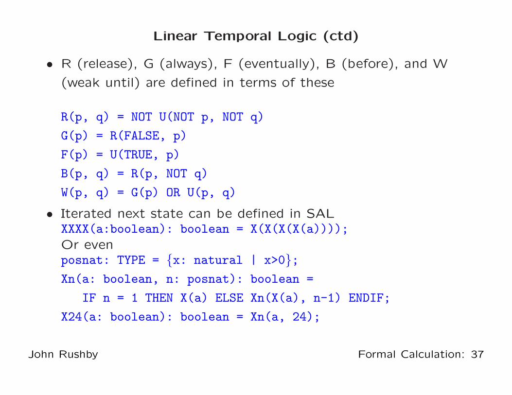
Linear Temporal Logic (ctd)
• R (release), G (always), F (eventually), B (before), and W
(weak until) are defined in terms of these
R(p, q) = NOT U(NOT p, NOT q)
G(p) = R(FALSE, p)
F(p) = U(TRUE, p)
B(p, q) = R(p, NOT q)
W(p, q) = G(p) OR U(p, q)
• Iterated next state can be defined in SALXXXX(a:boolean): boolean = X(X(X(X(a))));
Or evenposnat: TYPE = {x: natural | x>0};
Xn(a: boolean, n: posnat): boolean =
IF n = 1 THEN X(a) ELSE Xn(X(a), n-1) ENDIF;
X24(a: boolean): boolean = Xn(a, 24);
John Rushby Formal Calculation: 37
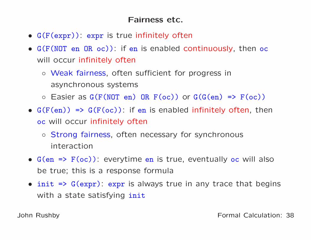
Fairness etc.
• G(F(expr)): expr is true infinitely often
• G(F(NOT en OR oc)): if en is enabled continuously, then oc
will occur infinitely often
◦ Weak fairness, often sufficient for progress in
asynchronous systems
◦ Easier as G(F(NOT en) OR F(oc)) or G(G(en) => F(oc))
• G(F(en)) => G(F(oc)): if en is enabled infinitely often, then
oc will occur infinitely often
◦ Strong fairness, often necessary for synchronous
interaction
• G(en => F(oc)): everytime en is true, eventually oc will also
be true; this is a response formula
• init => G(expr): expr is always true in any trace that begins
with a state satisfying init
John Rushby Formal Calculation: 38
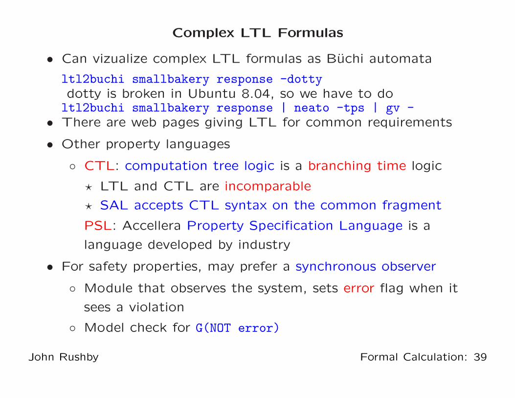
Complex LTL Formulas
• Can vizualize complex LTL formulas as Buchi automata
ltl2buchi smallbakery response -dottydotty is broken in Ubuntu 8.04, so we have to doltl2buchi smallbakery response | neato -tps | gv -
• There are web pages giving LTL for common requirements
• Other property languages
◦ CTL: computation tree logic is a branching time logic
⋆ LTL and CTL are incomparable
⋆ SAL accepts CTL syntax on the common fragment
PSL: Accellera Property Specification Language is a
language developed by industry
• For safety properties, may prefer a synchronous observer
◦ Module that observes the system, sets error flag when it
sees a violation
◦ Model check for G(NOT error)
John Rushby Formal Calculation: 39

From Symbolic to Bounded Model Checking
• Using a different example, sal-smc -v 3 om1 validity
◦ Oral Messages algorithm with n “relays”
• With 3 relays, 10,749,517,287 reachable states
• With 4 relays, 66,708,834,289,920 reachable states
• With 5 relays, run out of patience waiting for counterexample
• Bounded model checkers are specialized to finding
counterexamples
• Sometimes can handle bigger problems than SMC
John Rushby Formal Calculation: 40
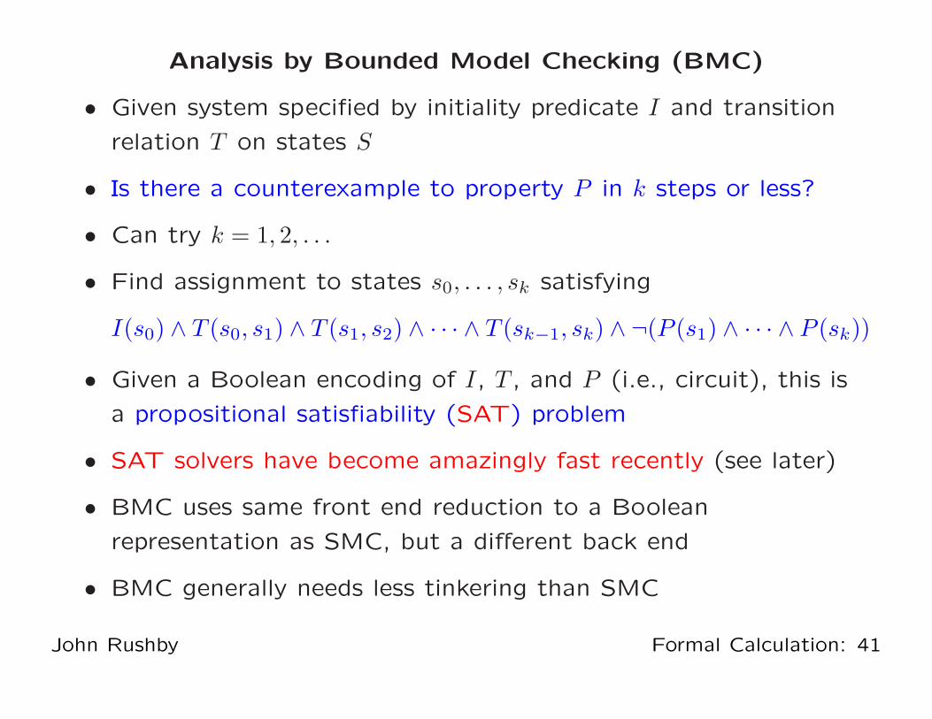
Analysis by Bounded Model Checking (BMC)
• Given system specified by initiality predicate I and transition
relation T on states S
• Is there a counterexample to property P in k steps or less?
• Can try k = 1, 2, . . .
• Find assignment to states s0, . . . , sk satisfying
I(s0) ∧ T (s0, s1) ∧ T (s1, s2) ∧ · · · ∧ T (sk−1, sk) ∧ ¬(P (s1) ∧ · · · ∧ P (sk))
• Given a Boolean encoding of I, T , and P (i.e., circuit), this is
a propositional satisfiability (SAT) problem
• SAT solvers have become amazingly fast recently (see later)
• BMC uses same front end reduction to a Boolean
representation as SMC, but a different back end
• BMC generally needs less tinkering than SMC
John Rushby Formal Calculation: 41
Bounded Model Checking with SAL
• We’ll use sal-bmc, Yices as its SAT solver (can use many
others); the depth k defaults to 10
• Finds the counterexample in the OM1 example in a few
secondssal-bmc -v 3 om1 validity -d 3
• And also all these examplessal-bmc -v 3 smallbakery liveness
sal-bmc -v 3 smallbakery bounded
sal-bmc -v 3 smallbakery unbounded -d 20
• But what about the true property?sal-bmc -v 3 smallbakery safety -d 20
Can keep increasing the depth, but what does that tell us?
John Rushby Formal Calculation: 42

Extending BMC to Verification
• We should require that s0, . . . , ska are distinct
◦ Otherwise there’s a shorter counterexample
• And we should not allow any but s0 to satisfy I
◦ Otherwise there’s a shorter counterexample
• If there’s no path of length k satisfying these two constraints,
and no counterexample has been found of length less than k,
then we have verified P
◦ By finding its finite diameter
• Seldom feasible in practice
John Rushby Formal Calculation: 43

Alternatively, Automated Induction via BMC
• Ordinary inductive invariance (for P):
Basis: I(s0) ⊃ P (s0)
Step: P (r0) ∧ T (r0, r1) ⊃ P (r1)
• Extend to induction of depth k:
Basis: No counterexample of length k or less
Step: P (r0)∧T (r0, r1)∧P (r1)∧ · · ·∧P (rk−1)∧T (rk−1, rk) ⊃ P (rk)
These are close relatives of the BMC formulas
• Induction for k = 2, 3, 4 . . . may succeed where k = 1 does not
• Note that counterexamples help debug invariant
• Can easily extend to use lemmas
John Rushby Formal Calculation: 44
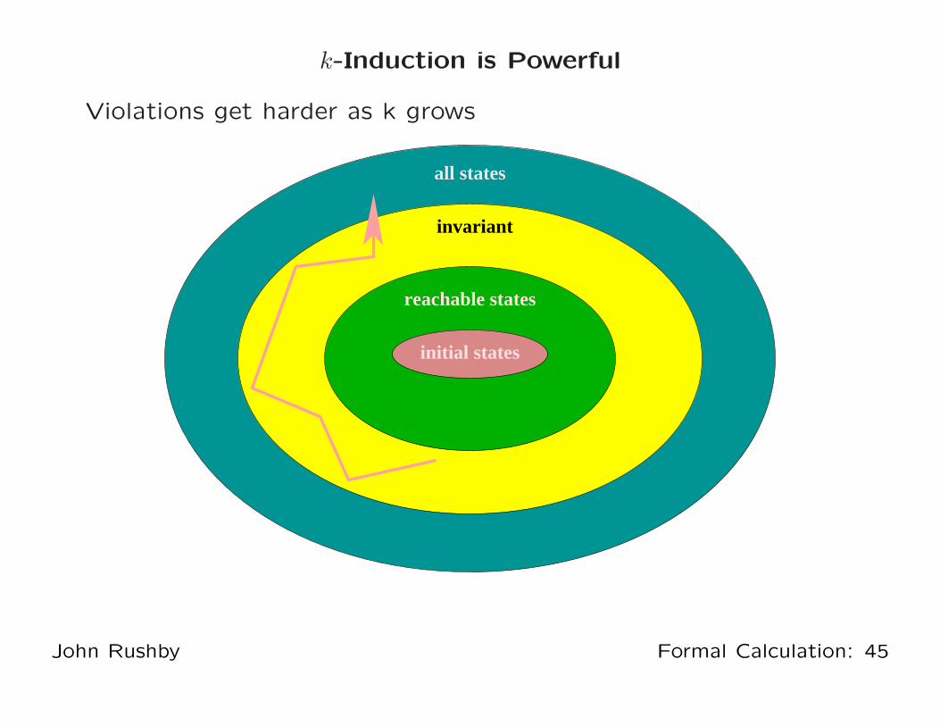
k-Induction is Powerful
Violations get harder as k grows
invariant
reachable states
all states
initial states
John Rushby Formal Calculation: 45

Verification by k-Induction
• Looking at an inductive counterexample can help suggest
lemmas (idea is to make the initial state infeasible)sal-bmc -v 3 -d 2 -i smallbakery safety -ice
• Here’s a simple lemma
aux: LEMMA system |- G((my_t = 0 => pc1 = idle)
AND (other_t = 0 => pc2 = idle));
• Can prove with sal-smc, or with 1-induction
sal-bmc -v 3 -d 1 -i smallbakery aux
• Can then verify safety with 2-induction using this lemma
sal-bmc -v 3 -d 2 -i smallbakery safety -l aux
John Rushby Formal Calculation: 46

Aside: BMC Can Also Solve Sudoku
John Rushby Formal Calculation: 47

Bounded Model Checking for Infinite State Systems
• We can discharge the BMC and k-induction efficiently for
Boolean encodings of finite state systems because SAT
solvers do efficient search
• If we could discharge these formulas over richer theories, we
could do BMC and k-induction for state machines over these
theories
• So how about if we combine a SAT solver with decision
procedures for useful theories like arithmetic?
• That’s what an SMT solver does (details later)
◦ Satisfiability Modulo Theories
• BMC using an SMT solver yields an infinite bounded model
checker
◦ i.e., a bounded model checker for infinite state systems
John Rushby Formal Calculation: 48
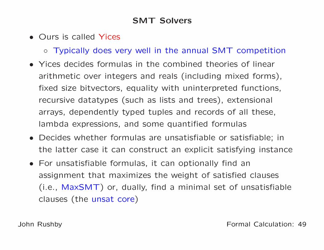
SMT Solvers
• Ours is called Yices
◦ Typically does very well in the annual SMT competition
• Yices decides formulas in the combined theories of linear
arithmetic over integers and reals (including mixed forms),
fixed size bitvectors, equality with uninterpreted functions,
recursive datatypes (such as lists and trees), extensional
arrays, dependently typed tuples and records of all these,
lambda expressions, and some quantified formulas
• Decides whether formulas are unsatisfiable or satisfiable; in
the latter case it can construct an explicit satisfying instance
• For unsatisfiable formulas, it can optionally find an
assignment that maximizes the weight of satisfied clauses
(i.e., MaxSMT) or, dually, find a minimal set of unsatisfiable
clauses (the unsat core)
John Rushby Formal Calculation: 49
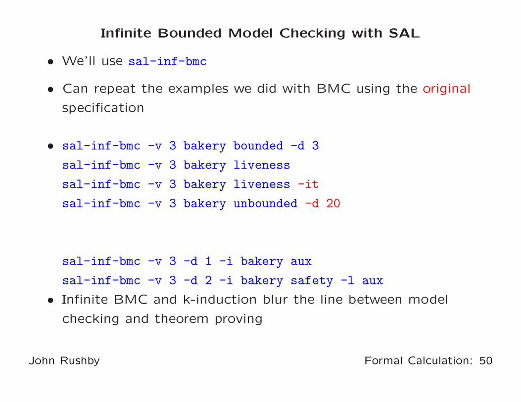
Infinite Bounded Model Checking with SAL
• We’ll use sal-inf-bmc
• Can repeat the examples we did with BMC using the original
specification
• sal-inf-bmc -v 3 bakery bounded -d 3
sal-inf-bmc -v 3 bakery liveness
sal-inf-bmc -v 3 bakery liveness -it
sal-inf-bmc -v 3 bakery unbounded -d 20
sal-inf-bmc -v 3 -d 1 -i bakery aux
sal-inf-bmc -v 3 -d 2 -i bakery safety -l aux
• Infinite BMC and k-induction blur the line between model
checking and theorem proving
John Rushby Formal Calculation: 50
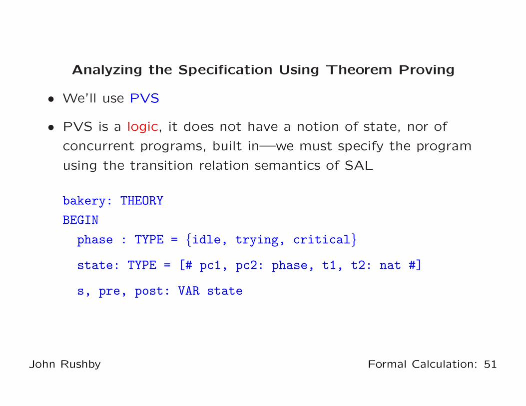
Analyzing the Specification Using Theorem Proving
• We’ll use PVS
• PVS is a logic, it does not have a notion of state, nor of
concurrent programs, built in—we must specify the program
using the transition relation semantics of SAL
bakery: THEORY
BEGIN
phase : TYPE = {idle, trying, critical}
state: TYPE = [# pc1, pc2: phase, t1, t2: nat #]
s, pre, post: VAR state
John Rushby Formal Calculation: 51
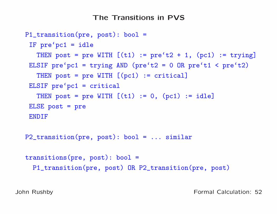
The Transitions in PVS
P1_transition(pre, post): bool =
IF pre‘pc1 = idle
THEN post = pre WITH [(t1) := pre‘t2 + 1, (pc1) := trying]
ELSIF pre‘pc1 = trying AND (pre‘t2 = 0 OR pre‘t1 < pre‘t2)
THEN post = pre WITH [(pc1) := critical]
ELSIF pre‘pc1 = critical
THEN post = pre WITH [(t1) := 0, (pc1) := idle]
ELSE post = pre
ENDIF
P2_transition(pre, post): bool = ... similar
transitions(pre, post): bool =
P1_transition(pre, post) OR P2_transition(pre, post)
John Rushby Formal Calculation: 52

Initialization and Invariant in PVS
init(s): bool = s‘pc1 = idle AND s‘pc2 = idle
AND s‘t1 = 0 AND s‘t2 = 0
safe(s): bool = NOT(s‘pc1 = critical AND s‘pc2 = critical)
% To prove that a property P is an invariant, we prove it is *inductive*
% This is similar to Amir Pnueli’s rule for Universal Invariance
% Except we strengthen the actual property rather than have an auxiliary
indinv(inv: pred[state]): bool =
FORALL s: init(s) => inv(s)
AND FORALL pre, post:
inv(pre) AND transitions(pre, post) => inv(post)
first_try: LEMMA indinv(safe)
John Rushby Formal Calculation: 53
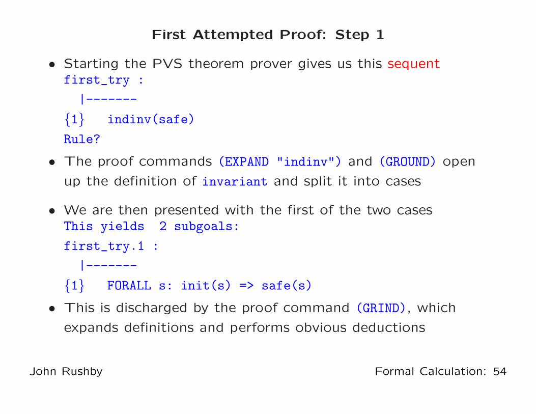
First Attempted Proof: Step 1
• Starting the PVS theorem prover gives us this sequentfirst_try :
|-------
{1} indinv(safe)
Rule?
• The proof commands (EXPAND "indinv") and (GROUND) open
up the definition of invariant and split it into cases
• We are then presented with the first of the two casesThis yields 2 subgoals:
first_try.1 :
|-------
{1} FORALL s: init(s) => safe(s)
• This is discharged by the proof command (GRIND), which
expands definitions and performs obvious deductions
John Rushby Formal Calculation: 54

First Attempted Proof: Step 2
• This completes the proof of first_try.1.
first_try.2 :
|-------
{1} FORALL pre, post:
safe(pre) AND transitions(pre, post) => safe(post)
• The commands (SKOSIMP), (EXPAND "transitions"), and
(GROUND) eliminate the quantification and split transitions
into separate cases for processes 1 and 2first_try.2.1 :
{-1} P1_transition(pre!1, post!1)
[-2] safe(pre!1)
|-------
[1] safe(post!1)
• (EXPAND "P1 transition") and (BDDSIMP) split the proof into
four cases according to the kind of step made by the process
John Rushby Formal Calculation: 55
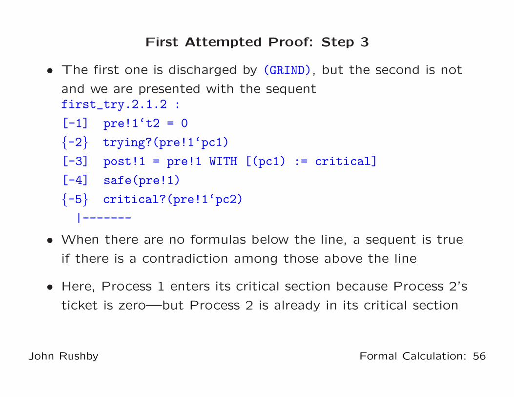
First Attempted Proof: Step 3
• The first one is discharged by (GRIND), but the second is not
and we are presented with the sequentfirst_try.2.1.2 :
[-1] pre!1‘t2 = 0
{-2} trying?(pre!1‘pc1)
[-3] post!1 = pre!1 WITH [(pc1) := critical]
[-4] safe(pre!1)
{-5} critical?(pre!1‘pc2)
|-------
• When there are no formulas below the line, a sequent is true
if there is a contradiction among those above the line
• Here, Process 1 enters its critical section because Process 2’s
ticket is zero—but Process 2 is already in its critical section
John Rushby Formal Calculation: 56
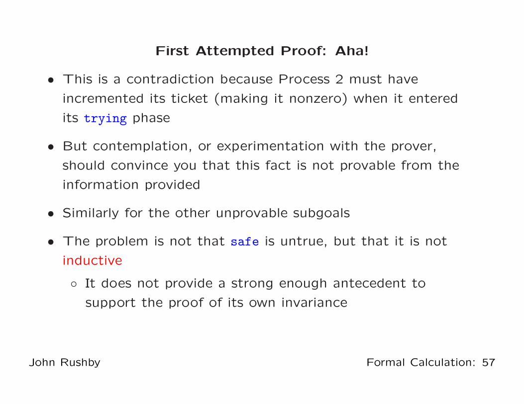
First Attempted Proof: Aha!
• This is a contradiction because Process 2 must have
incremented its ticket (making it nonzero) when it entered
its trying phase
• But contemplation, or experimentation with the prover,
should convince you that this fact is not provable from the
information provided
• Similarly for the other unprovable subgoals
• The problem is not that safe is untrue, but that it is not
inductive
◦ It does not provide a strong enough antecedent to
support the proof of its own invariance
John Rushby Formal Calculation: 57
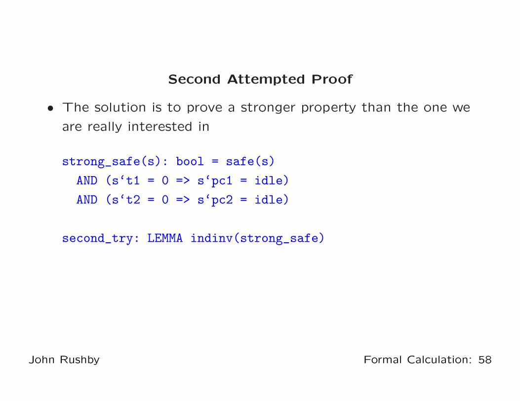
Second Attempted Proof
• The solution is to prove a stronger property than the one we
are really interested in
strong_safe(s): bool = safe(s)
AND (s‘t1 = 0 => s‘pc1 = idle)
AND (s‘t2 = 0 => s‘pc2 = idle)
second_try: LEMMA indinv(strong_safe)
John Rushby Formal Calculation: 58
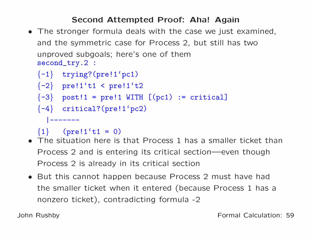
Second Attempted Proof: Aha! Again
• The stronger formula deals with the case we just examined,
and the symmetric case for Process 2, but still has two
unproved subgoals; here’s one of themsecond_try.2 :
{-1} trying?(pre!1‘pc1)
{-2} pre!1‘t1 < pre!1‘t2
{-3} post!1 = pre!1 WITH [(pc1) := critical]
{-4} critical?(pre!1‘pc2)
|-------
{1} (pre!1‘t1 = 0)• The situation here is that Process 1 has a smaller ticket than
Process 2 and is entering its critical section—even though
Process 2 is already in its critical section
• But this cannot happen because Process 2 must have had
the smaller ticket when it entered (because Process 1 has a
nonzero ticket), contradicting formula -2
John Rushby Formal Calculation: 59

Third Attempted Proof
• Again we need to strengthen the invariant to carry along this
fact
• inductive_safe(s):bool = strong_safe(s)
AND ((s‘pc1 = critical AND s‘pc2 = trying) => s‘t1 < s‘t2)
AND ((s‘pc2 = critical AND s‘pc1 = trying) => s‘t1 > s‘t2)
third_try: LEMMA indinv(inductive_safe)
• Finally, we have a invariant that is inductive—and is proved
with (GRIND)
John Rushby Formal Calculation: 60
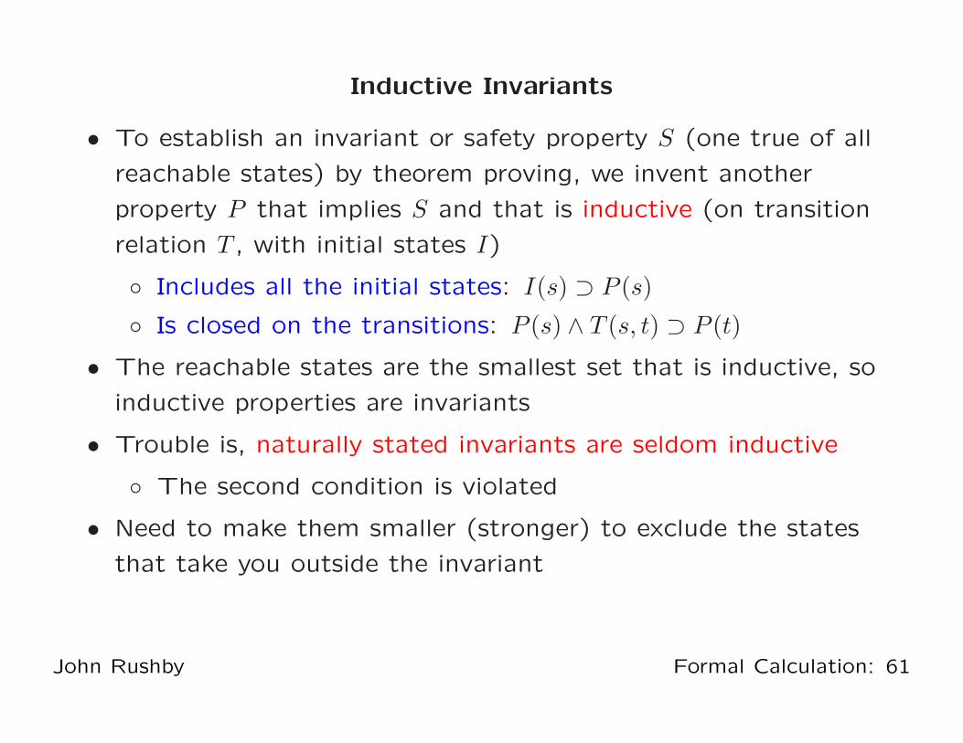
Inductive Invariants
• To establish an invariant or safety property S (one true of all
reachable states) by theorem proving, we invent another
property P that implies S and that is inductive (on transition
relation T , with initial states I)
◦ Includes all the initial states: I(s) ⊃ P (s)
◦ Is closed on the transitions: P (s) ∧ T (s, t) ⊃ P (t)
• The reachable states are the smallest set that is inductive, so
inductive properties are invariants
• Trouble is, naturally stated invariants are seldom inductive
◦ The second condition is violated
• Need to make them smaller (stronger) to exclude the states
that take you outside the invariant
John Rushby Formal Calculation: 61

Noninductive Invariants In Pictures
inductiveinvariant
invariant
reachable states
all states
initial states
John Rushby Formal Calculation: 62

Strengthening Invariants To Make Them Inductive
• Postulate a new invariant that excludes the states (so far
discovered) that take you outside the desired invariant
• Show that the conjunction of the new and the desired
invariant is inductive
• Iterate until success or exasperation
John Rushby Formal Calculation: 63

Inductive Invariants In Pictures
reachable states
all states
initial states
invariant
John Rushby Formal Calculation: 64

Strengthening Invariants To Make Them Inductive
• Iterate until success or exasperation
• Process can be made systematic
◦ Each strengthening was suggested by a failed proof
But is always tedious
• Bounded retransmission protocol required 57 such iterations
◦ Took a couple of months to complete
(Havelund and Shankar)
• Notice that each conjunct must itself be an invariant
(the very property we are trying to establish)
• Disjunctive invariants are an alternative for some problems
(see my CAV 2000 paper)
John Rushby Formal Calculation: 65
Pros and Cons of Theorem Proving
• Theorem proving can handle infinite state systems
• And accurate models
◦ Sometimes less says more–e.g., fault tolerance
• And general properties
(not just those expressible in temporal logic)
• But it’s hard (and not everyone finds it fun)
◦ Everything is possible but nothing is easy
◦ Especially strengthening of invariants
• Interaction focuses on proof, and idiosyncrasies of the prover,
not on the design being evaluated
◦ “Interactive theorem proving is a waste of human talent”
• It’s all or nothing
◦ No incremental return for incremental effort
John Rushby Formal Calculation: 66
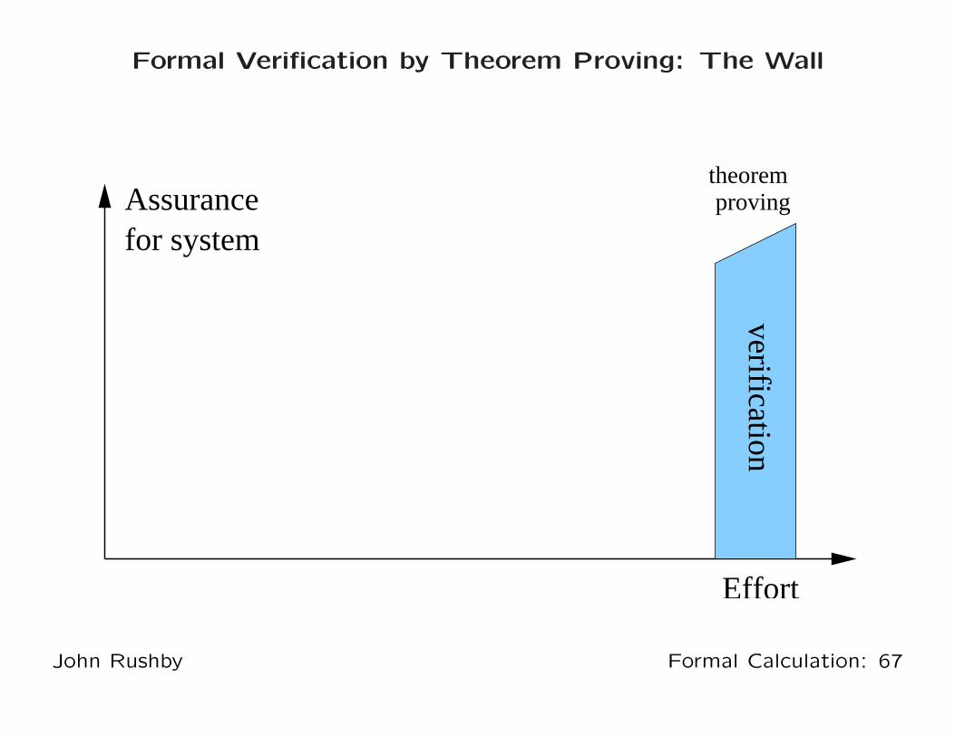
Formal Verification by Theorem Proving: The Wall
theoremproving
Effort
verificationfor systemAssurance
John Rushby Formal Calculation: 67

Aside: Design Choices in PVS
• Aside from the need to strengthen the invariant, PVS did OK
on this example (and does so on many more)
• We only used a fraction of its linguistic resources
◦ Higher-order logic with dependent predicate subtyping
◦ Recursive abstract data types and inductive types
◦ Parameterized theories and interpretations
◦ . . . and most of it is efficiently executable
• It automatically discharged subgoals by deciding properties
over abstract data types (enumeration types are a degenerate
case), integer arithmetic, record updates, prop’nl calculus
• In larger examples, it also has to choose when to open up a
definition, and when to apply a rewrite
• What makes PVS (and other verification systems) effective is
that it has tightly integrated automation for all of these
John Rushby Formal Calculation: 68

Top-Level Design Choices in PVS
• Specification language is a higher-order logic with subtyping
◦ Typechecking is undecidable: uses theorem proving
• User supplies top-level strategic guidance to the prover
◦ Invoking appropriate proof methods (induction etc.)
◦ Identifying necessary lemmas
◦ Suggesting case-splits
◦ Recovering when automation fails
• Automation takes care of the details, through a hierarchy of
techniques
1. Decision procedures
2. Rewriting (automates application of lemmas)
3. Heuristics (guess at case-splits, instantiations)
4. User-supplied strategies (cf. tactics in HOL)
John Rushby Formal Calculation: 69

Decision Procedures
Many important theories are decidable
• Propositional calculus
(a ∧ b) ∨ ¬a = a ⊃ b
• Equality with uninterpreted function symbols
x = y ∧ f(f(f(x))) = f(x) ⊃ f(f(f(f(f(y))))) = f(x)
• Function, record, and tuple updates
f with [(x) := y](z)def= if z = x then y else f(z)
• Linear Arithmetic (over integers and rationals)
x ≤ y ∧ x ≤ 1 − y ∧ 2 × x ≥ 1 ⊃ 4 × x = 2
But we need to decide combinations of theories
2 × car(x) − 3 × cdr(x) = f(cdr(x)) ⊃
f(cons(4 × car(x) − 2 × f(cdr(x)), y)) = f(cons(6 × cdr(x), y))
John Rushby Formal Calculation: 70
Combined Decision Procedures
• Some combinations of decidable theories are not decidable
◦ E.g., quantified theory of integer arithmetic (Presburger)
and equality over uninterpreted function symbols
• Need to make pragmatic compromises
◦ E.g., stick to ground (unquantified) theories and leave
quantification to heuristics at a higher level
• Two basic methods for combining decision procedures
◦ Nelson-Oppen: fewest restrictions
◦ Shostak: faster, yields a canonizer for combined theory
• Shostak’s method is used in PVS
◦ Over 20 years from first paper to fully correct treatment
◦ Now formally verified (in PVS)
by Jonathan Ford
John Rushby Formal Calculation: 71
Integrated Decision Procedures
• It’s not enough to have good decision procedures available to
discharge the leaves of a proof
◦ The endgame: PVS can use Yices for that
• They need to be used in simplification, which involves
recursive examination of subformulas: repeatedly adding,
subtracting, asserting, and denying subformulas
• And integrated with rewriting, where they used in matching
and (recursively) to decide conditions or top-level
if-then-else’s
• So the API to the decision procedures must be quite rich
John Rushby Formal Calculation: 72

Disruptive Innovation
Performance
Time
Low-end disruption is when low-end technology overtakes the
performance of high-end (Christensen)
John Rushby Formal Calculation: 73

SMT Solvers: Disruptive Innovation in Theorem Proving
• SMT stands for Satisfiability Modulo Theories
• SMT solvers extend decision procedures with the ability to
handle arbitrary propositional structure
◦ Traditionally, case analysis is handled heuristically in the
theorem prover front end
⋆ Have to be careful to avoid case explosion
◦ SMT solvers use the brute force of modern SAT solving
• Or, dually, they generalize SAT solving by adding the ability
to handle arithmetic and other decidable theories
• Application to verification
◦ Via bounded model checking and k-induction
John Rushby Formal Calculation: 74

SAT Solving
• Find satisfying assignment to a propositional logic formula
• Formula can be represented as a set of clauses
◦ In CNF: conjunction of disjunctions
◦ Find an assignment of truth values to variable that makes
at least one literal in each clause TRUE
◦ Literal: an atomic proposition A or its negation A
• Example: given following 4 clauses
◦ A,B
◦ C ,D
◦ E
◦ A, D, E
One solution is A, C, E, D
(A, D, E is not and cannot be extended to be one)
• Do this when there are 1,000,000s of variables and clauses
John Rushby Formal Calculation: 75
SAT Solvers
• SAT solving is the quintessential NP-complete problem
• But now amazingly fast in practice (most of the time)
◦ Breakthroughs (starting with Chaff) since 2001
⋆ Building on earlier innovations in SATO, GRASP
◦ Sustained improvements, honed by competition
• Has become a commodity technology
◦ MiniSAT is 700 SLOC
• Can think of it as massively effective search
◦ So use it when your problem can be formulated as SAT
• Used in bounded model checking and in AI planning
◦ Routine to handle 10300 states
John Rushby Formal Calculation: 76
SAT Plus Theories
• SAT can encode operations and relations on bounded
integers
◦ Using bitvector representation
◦ With adders etc. represented as Boolean circuits
And other finite data types and structures
• But cannot do not unbounded types (e.g., reals),
or infinite structures (e.g., queues, lists)
• And even bounded arithmetic can be slow when large
• There are fast decision procedures for these theories
• But their basic form works only on conjunctions
• General propositional structure requires case analysis
◦ Should use efficient search strategies of SAT solvers
That’s what an SMT solver does
John Rushby Formal Calculation: 77
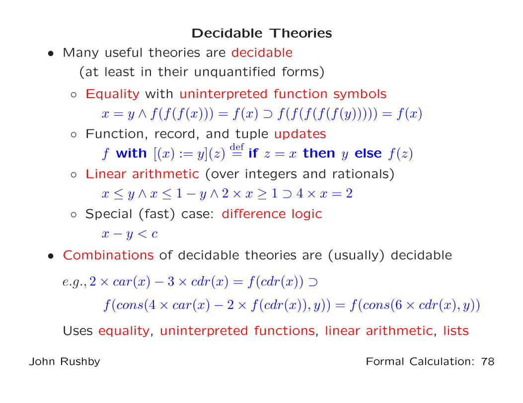
Decidable Theories
• Many useful theories are decidable
(at least in their unquantified forms)
◦ Equality with uninterpreted function symbols
x = y ∧ f(f(f(x))) = f(x) ⊃ f(f(f(f(f(y))))) = f(x)
◦ Function, record, and tuple updates
f with [(x) := y](z)def= if z = x then y else f(z)
◦ Linear arithmetic (over integers and rationals)
x ≤ y ∧ x ≤ 1 − y ∧ 2 × x ≥ 1 ⊃ 4 × x = 2
◦ Special (fast) case: difference logic
x − y < c
• Combinations of decidable theories are (usually) decidable
e.g., 2 × car(x) − 3 × cdr(x) = f(cdr(x)) ⊃
f(cons(4 × car(x) − 2 × f(cdr(x)), y)) = f(cons(6 × cdr(x), y))
Uses equality, uninterpreted functions, linear arithmetic, lists
John Rushby Formal Calculation: 78

SMT Solving
• Individual and combined decision procedures decide
conjunctions of formulas in their decided theories
• SMT allows general propositional structure
◦ e.g., (x ≤ y ∨ y = 5) ∧ (x < 0 ∨ y ≤ x) ∧ x 6= y
. . . possibly continued for 1000s of terms
• Should exploit search strategies of modern SAT solvers
• So replace the terms by propositional variables
◦ i.e., (A ∨ B) ∧ (C ∨ D) ∧ E
• Get a solution from a SAT solver (if none, we are done)
◦ e.g., A, D, E
• Restore the interpretation of variables and send the
conjunction to the core decision procedure
◦ i.e., x ≤ y ∧ y ≤ x ∧ x 6= y
John Rushby Formal Calculation: 79
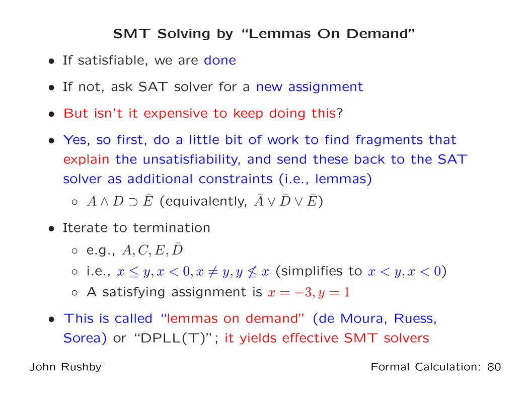
SMT Solving by “Lemmas On Demand”
• If satisfiable, we are done
• If not, ask SAT solver for a new assignment
• But isn’t it expensive to keep doing this?
• Yes, so first, do a little bit of work to find fragments that
explain the unsatisfiability, and send these back to the SAT
solver as additional constraints (i.e., lemmas)
◦ A ∧ D ⊃ E (equivalently, A ∨ D ∨ E)
• Iterate to termination
◦ e.g., A, C, E, D
◦ i.e., x ≤ y, x < 0, x 6= y, y 6≤ x (simplifies to x < y, x < 0)
◦ A satisfying assignment is x = −3, y = 1
• This is called “lemmas on demand” (de Moura, Ruess,
Sorea) or “DPLL(T)”; it yields effective SMT solvers
John Rushby Formal Calculation: 80
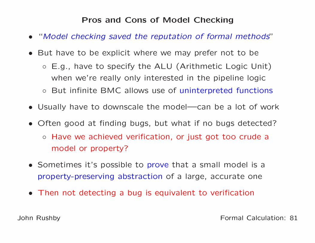
Pros and Cons of Model Checking
• “Model checking saved the reputation of formal methods”
• But have to be explicit where we may prefer not to be
◦ E.g., have to specify the ALU (Arithmetic Logic Unit)
when we’re really only interested in the pipeline logic
◦ But infinite BMC allows use of uninterpreted functions
• Usually have to downscale the model—can be a lot of work
• Often good at finding bugs, but what if no bugs detected?
◦ Have we achieved verification, or just got too crude a
model or property?
• Sometimes it’s possible to prove that a small model is a
property-preserving abstraction of a large, accurate one
• Then not detecting a bug is equivalent to verification
John Rushby Formal Calculation: 81

Model Checking: An Island
theoremproving
checkingmodel
Effort
refutation
verificationAssurancefor system
John Rushby Formal Calculation: 82

Combining Model Checking and Theorem Proving
• Model checking a downscaled instance is a useful prelude to
theorem proving the general case
• But a more interesting combination is to use model checking
as part of a proof for the general case
• One approach is to create a finite state property-preserving
abstraction of the original protocol
◦ Theorem proving shows abstraction preserves the property
◦ Model checking shows abstraction satisfies the property
Instead of proving indinv(safe), we invoke a model
checker to show abs system |- G(safe) [LTL]
Can actually do all of this within PVS, because it includes a
symbolic model checker (for CTL)
◦ Built on a decision procedure for finite µ-calculus
◦ We use it to prove init(s) => AG(safe)(s) [CTL]
John Rushby Formal Calculation: 83
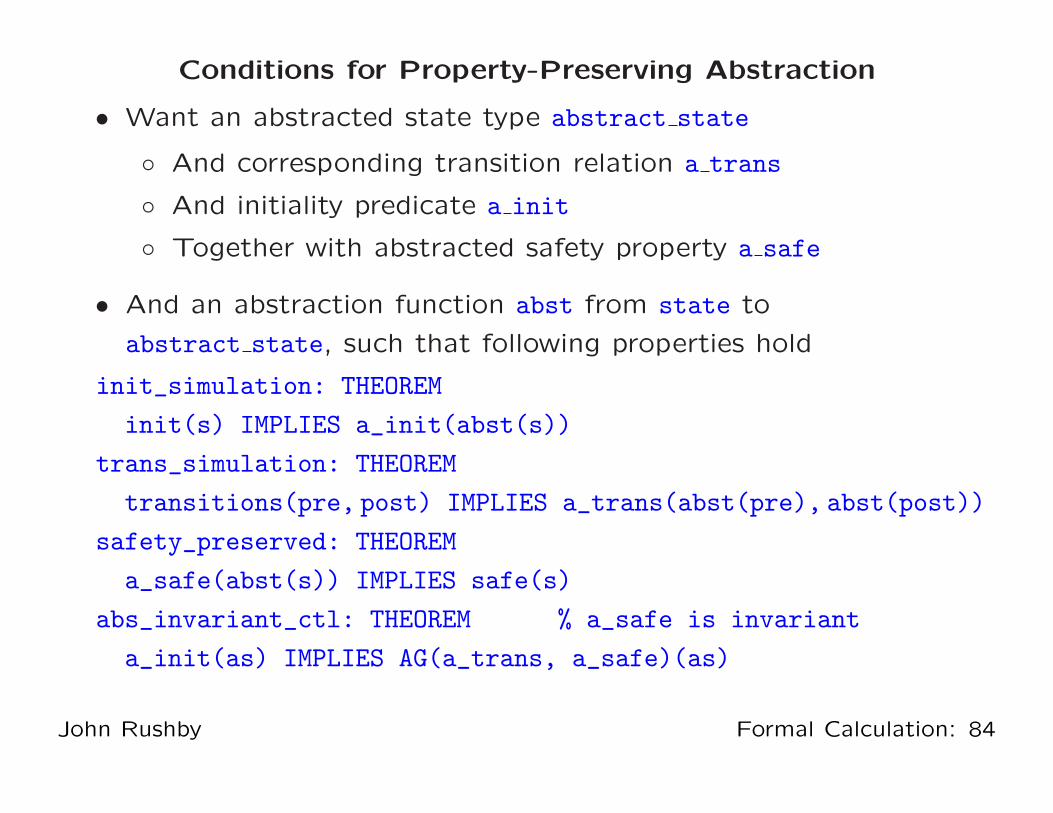
Conditions for Property-Preserving Abstraction
• Want an abstracted state type abstract state
◦ And corresponding transition relation a trans
◦ And initiality predicate a init
◦ Together with abstracted safety property a safe
• And an abstraction function abst from state to
abstract state, such that following properties hold
init_simulation: THEOREM
init(s) IMPLIES a_init(abst(s))
trans_simulation: THEOREM
transitions(pre, post) IMPLIES a_trans(abst(pre), abst(post))
safety_preserved: THEOREM
a_safe(abst(s)) IMPLIES safe(s)
abs_invariant_ctl: THEOREM % a_safe is invariant
a_init(as) IMPLIES AG(a_trans, a_safe)(as)
John Rushby Formal Calculation: 84

Abstracted Model
• It doesn’t matter to the protocol what the actual values of
the tickets are
• All that matters is whether or not each of them is zero, and
whether one is less than the other
• We can use Booleans to represent these relations
◦ This is called predicate abstraction
• So introduce the abstracted (finite) state typeabstract_state: TYPE =
[# pc1, pc2: phase,
t1_is_0, t2_is_0, t1_lt_t2: bool #]
as, a_pre, a_post: VAR abstract_state
John Rushby Formal Calculation: 85
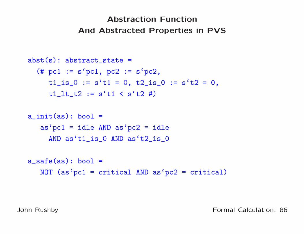
Abstraction Function
And Abstracted Properties in PVS
abst(s): abstract_state =
(# pc1 := s‘pc1, pc2 := s‘pc2,
t1_is_0 := s‘t1 = 0, t2_is_0 := s‘t2 = 0,
t1_lt_t2 := s‘t1 < s‘t2 #)
a_init(as): bool =
as‘pc1 = idle AND as‘pc2 = idle
AND as‘t1_is_0 AND as‘t2_is_0
a_safe(as): bool =
NOT (as‘pc1 = critical AND as‘pc2 = critical)
John Rushby Formal Calculation: 86

More of the Abstracted Specification
a_P1_transition(a_pre, a_post): bool =
IF a_pre‘pc1 = idle
THEN a_post = a_pre WITH [(t1_is_0) := false,
(t1_lt_t2) := false,
(pc1) := trying]
ELSIF a_pre‘pc1 = trying
AND (a_pre‘t2_is_0 OR a_pre‘t1_lt_t2)
THEN a_post = a_pre WITH [(pc1) := critical]
ELSIF a_pre‘pc1 = critical
THEN a_post = a_pre WITH [(t1_is_0) := true,
(t1_lt_t2) := NOT a_pre‘t2_is_0,
(pc1) := idle]
ELSE a_post = a_pre
ENDIF
John Rushby Formal Calculation: 87
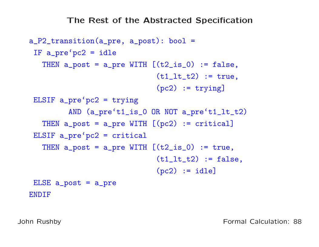
The Rest of the Abstracted Specification
a_P2_transition(a_pre, a_post): bool =
IF a_pre‘pc2 = idle
THEN a_post = a_pre WITH [(t2_is_0) := false,
(t1_lt_t2) := true,
(pc2) := trying]
ELSIF a_pre‘pc2 = trying
AND (a_pre‘t1_is_0 OR NOT a_pre‘t1_lt_t2)
THEN a_post = a_pre WITH [(pc2) := critical]
ELSIF a_pre‘pc2 = critical
THEN a_post = a_pre WITH [(t2_is_0) := true,
(t1_lt_t2) := false,
(pc2) := idle]
ELSE a_post = a_pre
ENDIF
John Rushby Formal Calculation: 88
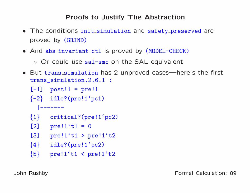
Proofs to Justify The Abstraction
• The conditions init simulation and safety preserved are
proved by (GRIND)
• And abs invariant ctl is proved by (MODEL-CHECK)
◦ Or could use sal-smc on the SAL equivalent
• But trans simulation has 2 unproved cases—here’s the firsttrans_simulation.2.6.1 :
[-1] post!1 = pre!1
{-2} idle?(pre!1‘pc1)
|-------
{1} critical?(pre!1‘pc2)
[2] pre!1‘t1 = 0
[3] pre!1‘t1 > pre!1‘t2
{4} idle?(pre!1‘pc2)
{5} pre!1‘t1 < pre!1‘t2
John Rushby Formal Calculation: 89

The Problem Justifying The Abstraction
• The problem here is that when the two tickets are equal but
nonzero, the concrete protocol drops through to the ELSE
case and requires the pre and post states to be the same
• But in the abstracted protocol, this situation can satisfy the
condition for Process 2 to enter its critical section
◦ Because NOT a pre‘t1 lt t2 abstracts pre‘t1 >= pre‘t2
rather than pre‘t1 > pre‘t2
• But this situation can never arise, because each ticket is
always incremented to be strictly greater than the other
• We can prove this as an invariantnot_eq(s): bool = s‘t1 = s‘t2 => s‘t1 = 0
extra: LEMMA indinv(not_eq)
• This is proved with (GRIND)
John Rushby Formal Calculation: 90
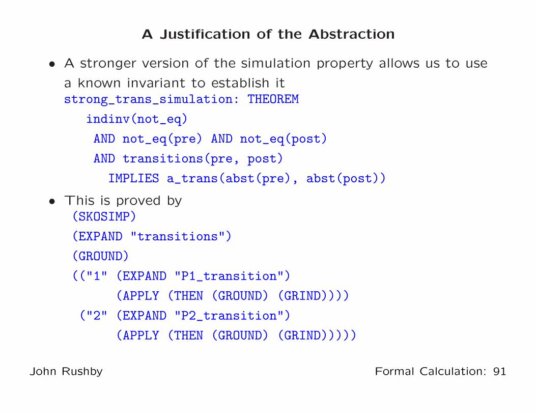
A Justification of the Abstraction
• A stronger version of the simulation property allows us to use
a known invariant to establish itstrong_trans_simulation: THEOREM
indinv(not_eq)
AND not_eq(pre) AND not_eq(post)
AND transitions(pre, post)
IMPLIES a_trans(abst(pre), abst(post))
• This is proved by(SKOSIMP)
(EXPAND "transitions")
(GROUND)
(("1" (EXPAND "P1_transition")
(APPLY (THEN (GROUND) (GRIND))))
("2" (EXPAND "P2_transition")
(APPLY (THEN (GROUND) (GRIND)))))
John Rushby Formal Calculation: 91
Pros and Cons of Manually-Constructed Abstractions
• Justifying the abstraction is usually almost as hard as proving
the property directly
• And generally requires auxiliary invariants
• Bounded retransmission protocol required 45 of the original
57 invariants to justify an abstraction
• But there’s the germ of an idea here
John Rushby Formal Calculation: 92
Abstraction Is The Bridge
Between Deductive and Algorithmic Methods
And Between Refutation and Verification
eorem Proving
straction mposition
eckingdel
John Rushby Formal Calculation: 93
Failure-Tolerant Theorem Proving
• Model checking is based on search
• Safe to do because the search space is bounded,
and efficient because we know its structure
• Verification systems (theorem provers aimed at verification)
tend to avoid search at the top level
◦ Too big a space to search, too little known about it
◦ When they do search, they have to rely on heuristics
◦ Which often fail
• Classical verification poses correctness as one “big theorem”
◦ So failure to prove it (when true) is catastrophic
• Instead, let’s try “failure-tolerant” theorem proving
◦ Prove lots of small theorems instead of one big one
◦ In a context where some failures can be tolerated
John Rushby Formal Calculation: 94

Contexts for Failure-Tolerant Theorem Proving
• Extended static checking (see later)
• Property preserving abstractions
◦ Instead of justifying an abstraction,
◦ Use deduction to calculate it
• Given a transition relation G on S and property P , a
property-preserving abstraction yields a transition relation G
on S and property P such that
G |= P ⇒ G |= P
Where G and P that are simple to analyze (e.g., finite state)
• A good abstraction typically (for safety properties)
introduces nondeterminism while preserving the property
• Note that abstraction is not the inverse of refinement
John Rushby Formal Calculation: 95
Calculating an Abstraction
• We need to figure out if we need a transition between any
pair of abstract states
• Given abstraction function φ : [S→S] we have
G(s1, s2) ⇔ ∃s1, s2 : s1 = φ(s1) ∧ s2 = φ(s2) ∧ G(s1, s2)
• We’ll use highly automated theorem proving on these
formulas: include transition iff the formula is proved
◦ There’s a chance we may fail to prove true formulas
◦ This will produce unsound abstractions
• So turn the problem around and calculate when we don’t
need a transition: omit transition iff the formula is proved
¬G(s1, s2) ⇔ ⊢ ∀s1, s2 : s1 6= φ(s1) ∨ s2 6= φ(s2) ∨ ¬G(s1, s2)
• Now theorem-proving failure affects accuracy, not soundness
John Rushby Formal Calculation: 96
Automated Abstraction
• The method described is automated in InVeSt
◦ An adjunct to PVS developed in conjunction with Verimag
• A different method (due to Saıdi and Shankar) is
implemented in PVS
◦ Exponentially more efficient
• The abstraction is specified in the proof command by giving
the concrete function or predicate that defines the value of
each abstract state variable
John Rushby Formal Calculation: 97
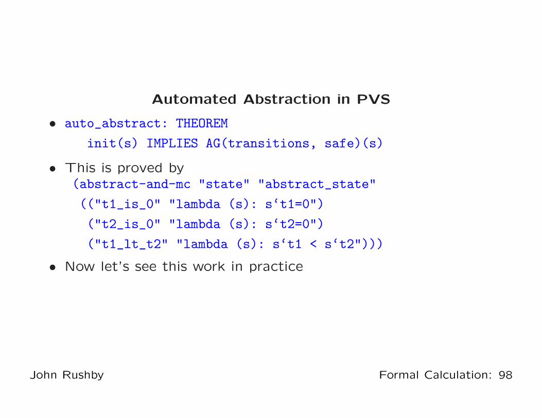
Automated Abstraction in PVS
• auto_abstract: THEOREM
init(s) IMPLIES AG(transitions, safe)(s)
• This is proved by(abstract-and-mc "state" "abstract_state"
(("t1_is_0" "lambda (s): s‘t1=0")
("t2_is_0" "lambda (s): s‘t2=0")
("t1_lt_t2" "lambda (s): s‘t1 < s‘t2")))
• Now let’s see this work in practice
John Rushby Formal Calculation: 98

Other Kinds of Abstraction
• We’ve seen predicate abstraction [Graf and Saıdi]
• I’ll briefly sketch data abstraction and hybrid abstraction
John Rushby Formal Calculation: 99

Data Abstraction [Cousot & Cousot]
• Replace concrete variable x over datatype C by an abstract
variable x′ over datatype A through a mapping h : [C→A]
• Examples: Parity, mod N , zero-nonzero, intervals,
cardinalities, {0, 1, many}, {empty, nonempty}
• Syntactically replace functions f on C by abstracted
functions f on A
• Given f : [C→C], construct f : [A→set [A]]:
(observe how data abstraction introduces nondeterminism)
b ∈ f(a) ⇔ ∃x : a = h(x) ∧ b = h(f(x))
b 6∈ f(a) ⇔ ⊢ ∀x : a = h(x) ⇒ b 6= h(f(x))
• Theorem-proving failure affects accuracy, not soundness
John Rushby Formal Calculation: 100

Data Abstraction Example
Replace natural numbers by {0, 1, many}
Calculate behavior of subtraction on {0, 1, many}
− 0 1 many
0 0 − −
1 1 0 −
many many {1, many} {0, 1, many}
0 /∈ (many − 1) iff ∀x ∈ {2, 3, 4, . . .} : x − 1 6= 0
John Rushby Formal Calculation: 101

Data Abstraction for Matlab (Hybrid Systems)
Stateflow
model
Simulink model
Mixed continuous/discrete (i.e., hybrid) system
John Rushby Formal Calculation: 102

Simulate One Trajectory at a Time
Stateflow
model
Simulink model
Just like testing: when have you done enough?
John Rushby Formal Calculation: 103
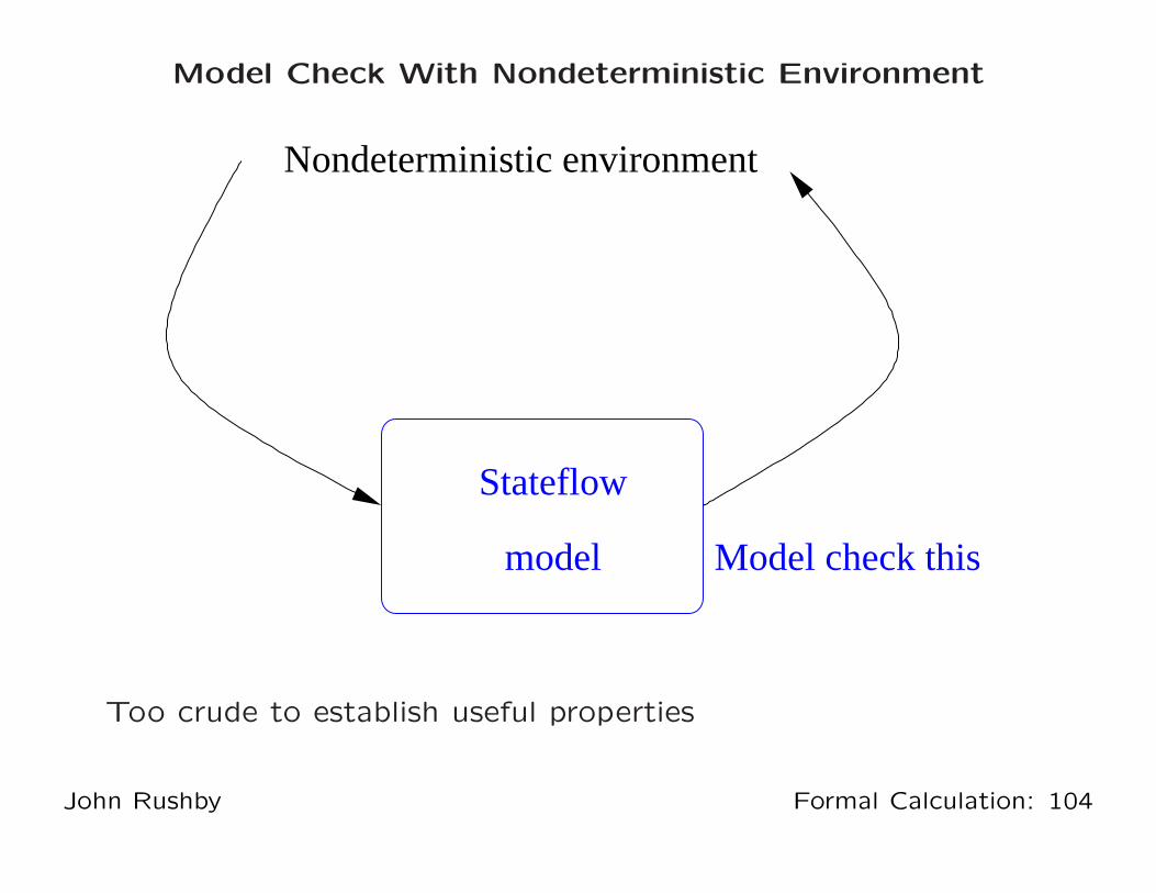
Model Check With Nondeterministic Environment
Stateflow
model Model check this
Nondeterministic environment
Too crude to establish useful properties
John Rushby Formal Calculation: 104
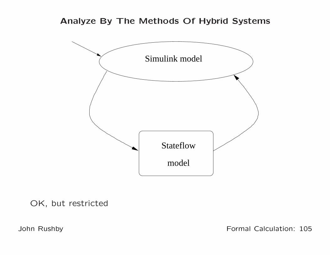
Analyze By The Methods Of Hybrid Systems
Stateflow
model
Simulink model
OK, but restricted
John Rushby Formal Calculation: 105

Model Check With Sound Discretization Of The
Continuous Environment
discrete
approximation
model
Stateflow
Model check all of this
Just right
John Rushby Formal Calculation: 106
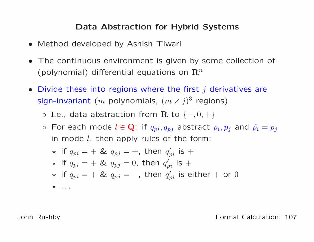
Data Abstraction for Hybrid Systems
• Method developed by Ashish Tiwari
• The continuous environment is given by some collection of
(polynomial) differential equations on Rn
• Divide these into regions where the first j derivatives are
sign-invariant (m polynomials, (m × j)3 regions)
◦ I.e., data abstraction from R to {−, 0, +}
◦ For each mode l ∈ Q: if qpi, qpj abstract pi, pj and pi = pj
in mode l, then apply rules of the form:
⋆ if qpi = + & qpj = +, then q′pi is +
⋆ if qpi = + & qpj = 0, then q′pi is +
⋆ if qpi = + & qpj = −, then q′pi is either + or 0
⋆ . . .
John Rushby Formal Calculation: 107
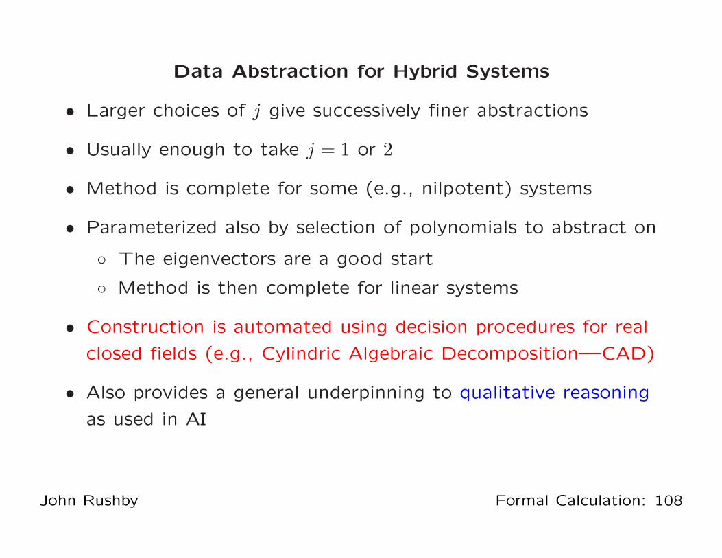
Data Abstraction for Hybrid Systems
• Larger choices of j give successively finer abstractions
• Usually enough to take j = 1 or 2
• Method is complete for some (e.g., nilpotent) systems
• Parameterized also by selection of polynomials to abstract on
◦ The eigenvectors are a good start
◦ Method is then complete for linear systems
• Construction is automated using decision procedures for real
closed fields (e.g., Cylindric Algebraic Decomposition—CAD)
• Also provides a general underpinning to qualitative reasoning
as used in AI
John Rushby Formal Calculation: 108
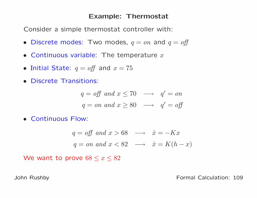
Example: Thermostat
Consider a simple thermostat controller with:
• Discrete modes: Two modes, q = on and q = off
• Continuous variable: The temperature x
• Initial State: q = off and x = 75
• Discrete Transitions:
q = off and x ≤ 70 −→ q′ = on
q = on and x ≥ 80 −→ q′ = off
• Continuous Flow:
q = off and x > 68 −→ x = −Kx
q = on and x < 82 −→ x = K(h − x)
We want to prove 68 ≤ x ≤ 82
John Rushby Formal Calculation: 109
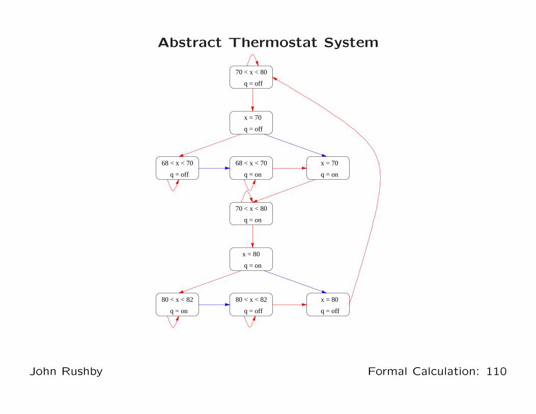
Abstract Thermostat System
70 < x < 80
q = off
68 < x < 70
q = on
q = off
70 < x < 80
x = 70
q = on
q = on
x = 80
80 < x < 82
q = off
68 < x < 70
q = on
q = onq = off
x = 70
80 < x < 82 x = 80
q = off
John Rushby Formal Calculation: 110

Pros and Cons of Automated Abstraction
• Good match between local theorem proving,
and global model checking
• Quality of the abstraction depends on information provided
by the user (predicates, polynomials etc.)
◦ It’s easier to guess useful predicates than invariants
◦ Can guess additional ones if inadequate
◦ Or let counterexamples suggest refinements (CEGAR)
⋆ A general approach can be discerned here: find quick
solutions and fix them up, rather than deliberate in
hope of finding good solutions
And the deductive power applied
◦ Which may increase if provided with known invariants
John Rushby Formal Calculation: 111

Truly Integrated, Iterated Analysis!
• Recast the goal as one of calculating and accumulating
properties about a design (symbolic analysis)
• Rather than just verifying or refuting a specific property
• Properties convey information and insight, and provide
leverage to construct new abstractions
◦ And hence more properties
• Requires restructuring of verification tools
◦ So that many work together
◦ And so that they return symbolic values and properties
rather than just yes/no results of verifications
• This is what SAL is about: Symbolic Analysis Laboratory
◦ Next generation will have a tool bus
John Rushby Formal Calculation: 112

Integrated, Iterated Analysis
John Rushby Formal Calculation: 113

Refutation and Verification
• By allowing unsound abstractions
G |= P 6⇒ G |= P
We can do refutation as well as verification
• Then, by selecting abstractions (sound/unsound) and
properties (little/big) we can fill in the space between
refutation and verification
• Refutation lowers the barrier to entry
• Provides economic incentive: discovery of high value bugs
◦ Can estimate the cost of each bug found
◦ And can directly compare with other technologies
• Yet allows smooth transition to verification
John Rushby Formal Calculation: 114

From Refutation To Verification
checkingmodel
provingtheorem
& inf−BMC
Effort
Assurancefor system
refutation
verification
automated abstraction
John Rushby Formal Calculation: 115
Filling the Remaining Gap
• Model checking for refutation and (via automated
abstraction and inf-BMC) for verification imposes a much
smaller barrier to adoption than old-style formal verification
• But the barrier is still there
• What about really low cost/low threat kinds of formal
analysis?
• Make the formal methods disappear inside traditional tools
and methods
◦ We call these invisible formal methods
◦ And it’s where a lot of the action and opportunity is
John Rushby Formal Calculation: 116
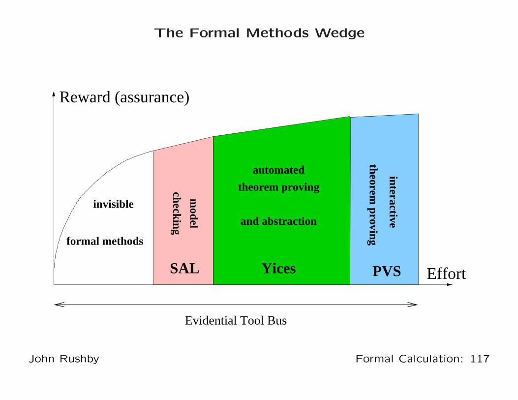
The Formal Methods Wedge
theorem proving
interactive
model
checking
Reward (assurance)
PVSSAL
automated
theorem proving
and abstraction
invisible
formal methods
EffortYices
Evidential Tool Bus
John Rushby Formal Calculation: 117
Examples of Invisible Formal Methods
Stronger Checking in Traditional Tools
• Various forms of extended static checking
◦ Failed proof generates a possibly spurious warning
• Static analysis: typestate, shape analysis, abstract
interpretation etc.
• PVS-like type system (predicate subtypes) for any language
◦ Traditional type systems have to be trivially decidable
◦ But can gain enormous error detection by adding a
component that requires theorem proving (lots of small
theorems, failure generates a spurious warning)
• The verifying compiler (aka. verified systems roadmap)
John Rushby Formal Calculation: 118

Examples of Invisible Formal Methods
Better Tools for Traditional Activities
• Statechart/Stateflow property checkers
(cf. Reactis, Honeywell, SRI, Mathworks)
◦ Show me a path that activates this state
◦ Can this state and that be active simultaneously?
• Checker synthesizers (cf. IBM FOCS)
• Completeness/Consistency checkers for tabular specifications
(cf. Ontario Hydro, RSML, SCR)
• Test case generators (cf. Verimag/IRISA TGV and STG,
SAL-ATG)
There’s an entire industry in this space, with many companies
make a living from modest technology (but very good
understanding of their markets)
John Rushby Formal Calculation: 119
Static Program Analysis
John Rushby Formal Calculation: 120

The Bug That Stopped The Zunes
Real time clock sets days to number of days since 1 Jan 1980
year = ORIGINYEAR; /* = 1980 */
while (days > 365) {
if (IsLeapYear(year)) {
if (days > 366) {
days -= 366;
year += 1;
} else... loops forever on last day of a leap year
} else {
days -= 365;
year += 1;
}
}
Coverage-based testing will find this
John Rushby Formal Calculation: 121

A Hasty Fix
while (days > 365) {
if (IsLeapYear(year)) {
if (days > 365) {
days -= 366;
year += 1;
}
} else {
days -= 365;
year += 1;
}
}
• Fixes the loop but now days can end up as zero
• Coverage-based testing might not find this
• Boundary condition testing would
• But I think the point is clear. . .
John Rushby Formal Calculation: 122
The Problem With Testing
• Is that it only samples the set of possible behaviors
• And unlike physical systems (where many engineers gained
their experience), software systems are discontinuous
• There is no sound basis for extrapolating from tested to
untested cases
• So we need to consider all possible cases. . . how is this
possible?
• It’s possible with symbolic methods
• Cf. x2 − y2 = (x − y)(x + y) vs. 5*5-3*3 = (5-3)*(5+3)
• Static Analysis is about totally automated ways to do this
John Rushby Formal Calculation: 123
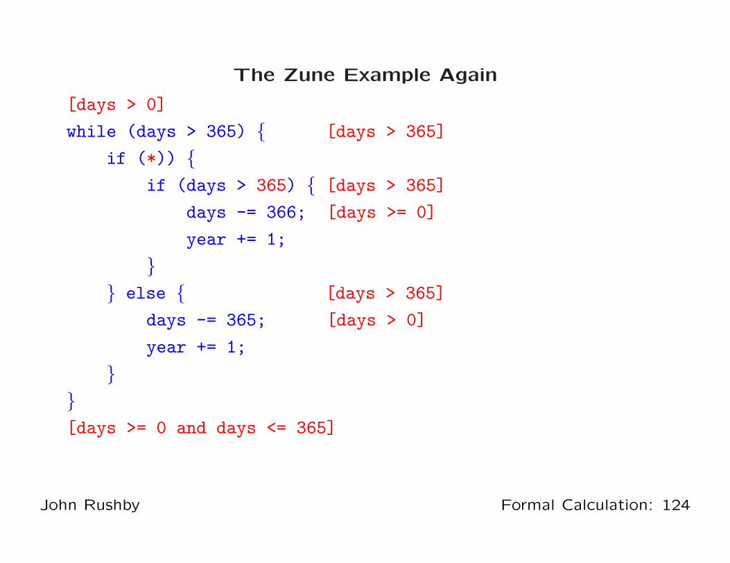
The Zune Example Again
[days > 0]
while (days > 365) { [days > 365]
if (*)) {
if (days > 365) { [days > 365]
days -= 366; [days >= 0]
year += 1;
}
} else { [days > 365]
days -= 365; [days > 0]
year += 1;
}
}
[days >= 0 and days <= 365]
John Rushby Formal Calculation: 124
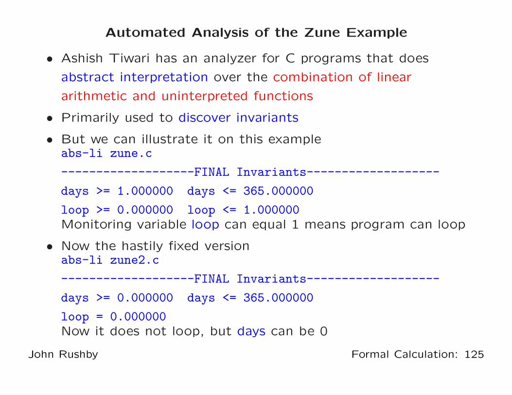
Automated Analysis of the Zune Example
• Ashish Tiwari has an analyzer for C programs that does
abstract interpretation over the combination of linear
arithmetic and uninterpreted functions
• Primarily used to discover invariants
• But we can illustrate it on this exampleabs-li zune.c
-------------------FINAL Invariants-------------------
days >= 1.000000 days <= 365.000000
loop >= 0.000000 loop <= 1.000000Monitoring variable loop can equal 1 means program can loop
• Now the hastily fixed versionabs-li zune2.c
-------------------FINAL Invariants-------------------
days >= 0.000000 days <= 365.000000
loop = 0.000000Now it does not loop, but days can be 0
John Rushby Formal Calculation: 125

Approximations
• We were lucky that we could do the previous example with
full symbolic arithmetic
• Usually, the formulas get bigger and bigger as we accumulate
information from loop iterations (we’ll see an example later)
• So it’s common to approximate or abstract information to
try and keep the formulas manageable
• Here, instead of the natural numbers 0, 1, 2, . . . , we could
use
◦ zero, small, big
◦ Where big abstracts everything bigger than 365, small is
everything from 1 to 365, and zero is 0
◦ Arithmetic becomes nondeterministic
⋆ e.g., small+small = small | big
John Rushby Formal Calculation: 126
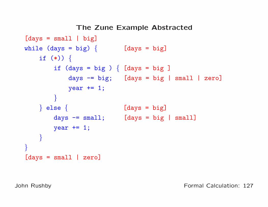
The Zune Example Abstracted
[days = small | big]
while (days = big) { [days = big]
if (*)) {
if (days = big ) { [days = big ]
days -= big; [days = big | small | zero]
year += 1;
}
} else { [days = big]
days -= small; [days = big | small]
year += 1;
}
}
[days = small | zero]
John Rushby Formal Calculation: 127

The Zune Example Abstracted Again
Suppose we abstracted to {negative, zero, positive}
[days = positive]
while (days = positive) { [days = positive]
if (*)) {
if (days = positive ) { [days = positive ]
days -= positive; [days = negative | zero | positive]
year += 1;
}
} else { [days = positive]
days -= positive; [days = negative | zero | positive]
year += 1;
} }
[days = negative | zero]
We’ve lost too much information: have a false alarm that days
can go negative (pointer analysis is sometimes this crude)
John Rushby Formal Calculation: 128

We Have To Approximate, But There’s A Price
• It’s no accident that we sometimes lose precision
• Rice’s Theorem says there are inherent limits on what can be
accomplished by automated analysis of programs
◦ Sound (miss no errors)
◦ Complete (no false alarms)
◦ Automatic
◦ Allow arbitrary (unbounded) memory structures
◦ Final results
Choose at most 4 of the 5
John Rushby Formal Calculation: 129

Approximations
reachable states
approximation
Sound approximations include all the behaviors and reachable
states of the real system, but are easier to compute
John Rushby Formal Calculation: 130
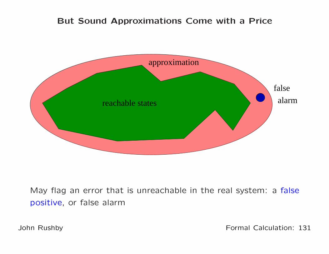
But Sound Approximations Come with a Price
reachable states
approximation
alarm
false
May flag an error that is unreachable in the real system: a false
positive, or false alarm
John Rushby Formal Calculation: 131

Unsound Approximations Come with a Price, Too
reachable states
underapproximation
false
negative
Can miss real errors: a false negative
John Rushby Formal Calculation: 132

Predicate Abstraction
• The Zune example used data abstraction
◦ A kind of abstract interpretation
• Replaces variables of complex data types by simpler
(often finite) ones
◦ e.g., integers replaced by {negative, zero, positive}
• But sometimes this doesn’t work
◦ Just replaces individual variables
◦ Often its the relationship between variables that matters
• Predicate abstraction replaces some relationships (predicates)
by Boolean variables
John Rushby Formal Calculation: 133

Another Example
start with r unlocked
do {
lock(r)
old = new
if (*) {
unlock(r)
new++
}
}
while old != new
want r to be locked at this point
unlock(r)
John Rushby Formal Calculation: 134

Abstracted Example
The significant relationship seems to be old == new
Replace this by eq, throw away old and new
[!locked]
do {
lock(r) [locked]
eq = true [locked, eq]
if (*) {
unlock(r) [!locked, eq]
eq = false [!locked, !eq]
}
} [locked, eq] or [!locked, !eq]
while not eq
[locked, eq]
unlock(r)
John Rushby Formal Calculation: 135

Yet Another Example
z := n; x := 0; y := 0;
while (z > 0) {
if (*) {
x := x+1;
z := z-1;
} else {
y := y+1;
z := z-1;
}
}
want y!= 0, given x != z, n > 0
• The invariant needed is x + y + z = n
• But neither this nor its fragments appear in the program or
the desired property
John Rushby Formal Calculation: 136

Let’s Just Go Ahead
First time into the loop
[n > 0]
z := n; x := 0; y := 0;
while (z > 0) { [x = 0, y = 0, z = n]
if (*) {
x := x+1;
z := z-1; [x = 1, y = 0, z = n-1]
} else {
y := y+1;
z := z-1; [x = 0, y = 1, z = n-1]
} [x = 1, y = 0, z = n-1] or [x = 0, y = 1, z = n-1]
}
Next time around the loop we’ll have 4 disjuncts, then 8, then
16, and so on
This won’t get us anywhere useful
John Rushby Formal Calculation: 137
Widening the Abstraction
• We could try eliminate disjuncts
• Look for a conjunction that is implied by each of the disjuncts
• One such is [x+y = 1, z = n-1]
• Then we’d need to do the same thing with
[x+y = 1, z = n-1] or [x = 0, y = 0, z = n]
• That gives [x + y + z = n]
• There are techniques that can do this automatically
• This is where a lot of the research action is
John Rushby Formal Calculation: 138

Tradeoffs
• We’re trying to guarantee absence of errors in a certain class
• Equivalently, trying to verify properties of a certain class
• Terminology is in terms of finding errors
TP True Positive: found a real error
FP False Positive: false alarm
TN True Negative: no error, no alarm—OK
FN False Negative: missed error
• Then we have
Sound: no false negatives
Recall: TP/(TP+FN) measures how (un)sound
TP+FN is number of real errors
Complete: no false alarms
Precision: TP/(TP+FP) measures how (in)complete
TP+FP is number of alarms
John Rushby Formal Calculation: 139
Tradeoff Space
• Basic tradeoff is between soundness and completeness
• For assurance, we need soundness
◦ When told there are no errors, there must be none
So have to accept false alarms
• But the main market for static analysis is bug finding in
general-purpose software, where they aim merely to reduce
the number of bugs, not to eliminate them
• Their general customers will not tolerate many false alarms,
so tool vendors give up soundness
• Will consider the implications later
• Other tradeoffs are possible
◦ Give up full automation: e.g., require user annotation
John Rushby Formal Calculation: 140
Tradeoffs In Practice
Testing is complete but unsound
Spark Ada with its Examiner is sound but not fully
automatic
Abstract Interpretation (e.g., PolySpace) is sound but
incomplete, and may not terminate
• Astree is pragmatically complete for its domain
Pattern matchers (e.g. Lint, Findbugs) are not based on
semantics of program execution, neither sound nor complete
• But pragmatically effective for bug finding
Commercial tools (e.g., Coverity, Code Sonar, Fortify,
KlocWork, LDRA) are neither sound nor complete
• Pragmatically effective
• Different tools use different methods, have different
capabilities, make different tradeoffs
John Rushby Formal Calculation: 141

Properties Checked
• The properties checked are usually implicit
◦ e.g., uninitialized variables, divide by zero (and other
exceptions), null pointer dereference, buffer overrun
• Much of this is compensating for deficiencies of C and C++
◦ Some tools support Ada, Java, not much for MBD
◦ But Mathworks has Design Verifier for Simulink
• Some tools support user-specified checks, but. . .
• Some tools look at resources
◦ e.g., memory leaks, locks (not freed, freed twice, use
after free)
• Some (e.g., AbsInt) can do quantitative analysis
◦ e.g., worst case execution time, maximum stack height
John Rushby Formal Calculation: 142
Real Software
• It’s not enough to check individual programs
• Need information from calls to procedures, subroutines
◦ Analyze each in isolation, then produce a procedure
summary for use by others
• Need summaries for libraries, operating system calls
• Analyzer must integrate with the build process
• Must present the information in a useful and attractive way
• Much of the engineering in commercial tools goes here
John Rushby Formal Calculation: 143
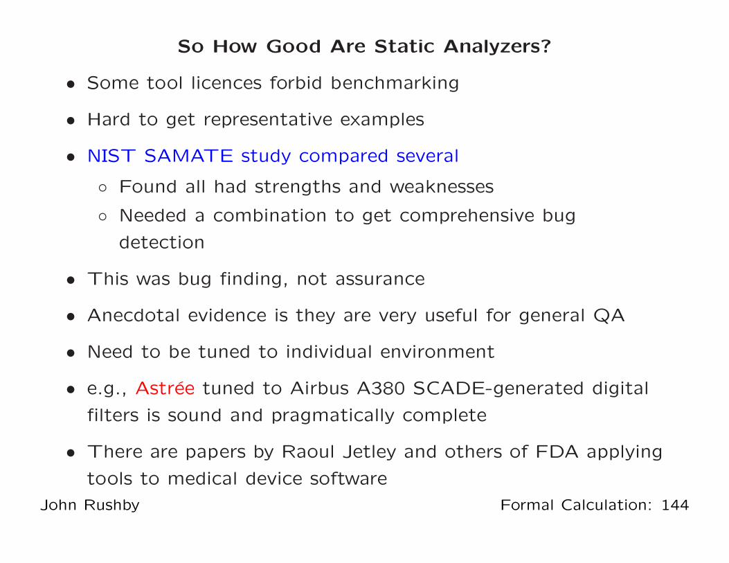
So How Good Are Static Analyzers?
• Some tool licences forbid benchmarking
• Hard to get representative examples
• NIST SAMATE study compared several
◦ Found all had strengths and weaknesses
◦ Needed a combination to get comprehensive bug
detection
• This was bug finding, not assurance
• Anecdotal evidence is they are very useful for general QA
• Need to be tuned to individual environment
• e.g., Astree tuned to Airbus A380 SCADE-generated digital
filters is sound and pragmatically complete
• There are papers by Raoul Jetley and others of FDA applying
tools to medical device software
John Rushby Formal Calculation: 144
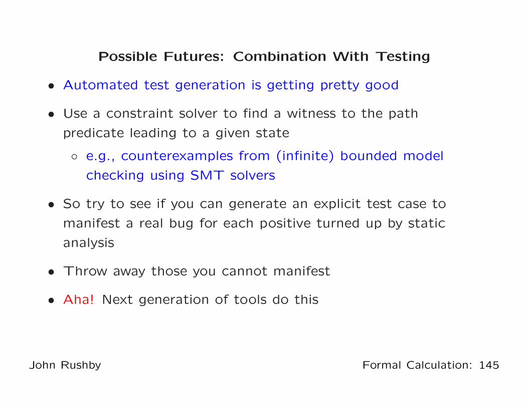
Possible Futures: Combination With Testing
• Automated test generation is getting pretty good
• Use a constraint solver to find a witness to the path
predicate leading to a given state
◦ e.g., counterexamples from (infinite) bounded model
checking using SMT solvers
• So try to see if you can generate an explicit test case to
manifest a real bug for each positive turned up by static
analysis
• Throw away those you cannot manifest
• Aha! Next generation of tools do this
John Rushby Formal Calculation: 145

Automated Test Generation
John Rushby Formal Calculation: 146

Test Generation
• Observe that a counterexample to an assertion: “control
cannot reach this point” is a structural test case
• So BMC can be used for automated test generation
• Actually, a customized combination of SMC and BMC works
best
◦ Use SMC to reach first control point, then use BMC to
extend to further control points
◦ Get long tests that probe deep into the system
◦ Can add test purposes that constrain the kinds of tests
generated
⋆ e.g., Change the gear input by 1 at every step
◦ Easily built because checkers are scriptable (in Scheme)
John Rushby Formal Calculation: 147

Core Of The SAL-ATG Test Generation Script(define (extend-search module goal-list
path scan prune innerslice start step stop)
(let ((new-goal-list (if prune (goal-reduce scan goal-list path)
(minimal-goal-reduce scan goal-list path))))
(cond ((null? new-goal-list) (cons ’() path))
((> start stop) (cons new-goal-list path))
(else
(let* ((goal (list->goal new-goal-list module))
(mod (if innerslice
(sal-module/slice-for module goal) module))
(new-path
(let loop ((depth start))
(cond ((> depth stop) ’())
((sal-bmc/extend-path
path mod goal depth ’ics))
(else (loop (+ depth step)))))))
(if (pair? new-path)
(extend-search mod new-goal-list new-path scan
prune innerslice start step stop)
(cons new-goal-list path)))))))
John Rushby Formal Calculation: 148

Outer Loop Of The SAL-ATG Test Generation Script
(define (iterative-search module goal-list
scan prune slice innerslice bmcinit start step stop)
(let* ((goal (list->goal goal-list module))
(mod (if slice (sal-module/slice-for module goal) module))
(path (if bmcinit
(sal-bmc/find-path-from-initial-state
mod goal bmcinit ’ics)
(sal-smc/find-path-from-initial-state mod goal))))
(if path
(extend-search mod goal-list path scan prune
innerslice start step stop)
#f)))
John Rushby Formal Calculation: 149

Example: Shift Scheduler in StateFlow
[gear ==3]
[gear == 3]
[V <= shift_speed_32]
[gear == 1]
[V > shift_speed_23]
[V > shift_speed_34]
[V <= shift_speed_21] [V > shift_speed_12] [V <= shift_speed_43]
[V > shift_speed_23]
[V <= shift_speed_23]
[gear == 2]
[gear == 4]
[V <= shift_speed_43]
[V > shift_speed_34]
[gear == 2][V <= shift_speed_21]
[V > shift_speed_12]
third_gearentry: to_gear=3;first_gear
entry: to_gear = 1;
transition12
[ctr > DELAY]
shift_pending_aentry: ctr=0; to_gear=1;during: ctr=ctr+1;
shifting_aentry: to_gear=2;
transition23
[ctr > DELAY]
shift_pending2entry: ctr=0; to_gear=2;during: ctr=ctr + 1;
shifting2entry: to_gear=3;
transition34
[ctr > DELAY]
shift_pending3entry: ctr=0; to_gear=3;during: ctr = ctr+1;
shifting3entry: to_gear=4;
fourth_gearentry: to_gear =4;
second_gearentry: to_gear=2;
transition43
[ctr > DELAY]
shift_pending_dentry: ctr=0; to_gear =4;during: ctr=ctr+1;
shifting_dentry: to_gear=3;
transition32
[ctr > DELAY]
shift_pending_centry: ctr=0; to_gear=3;during: ctr=ctr+1;
shifting_centry: to_gear=2;
transition21
[ctr > DELAY]
shift_pending_bentry: ctr=0; to_gear=2;during: ctr = ctr+1;
shifting_bentry: to_gear=1;
Demo: sal-atg -v 3 trans ga monitored system
trans ga goals.scm -ed 15 –incremental –testpurpose
John Rushby Formal Calculation: 150
Timed Systems
John Rushby Formal Calculation: 151

Verification of Real Time Programs
• Continuous time excludes automation by finite state methods
• Timed automata methods (e.g., Uppaal)
◦ Handle continuous time
◦ But are defeated by the case explosion when (discrete)
faults are considered as well
• SMT solvers can handle both dimensions
◦ With discrete time, can have a clock module that
advances time one tick at a time
⋆ Each module sets a timeout, waits for the clock to
reach that value, then does its thing, and repeats
◦ Better: move the timeout to the clock module and let it
advance time all the way to the next timeout
⋆ These are Timeout Automata (Dutertre and Sorea):
and they work for continuous time
John Rushby Formal Calculation: 152
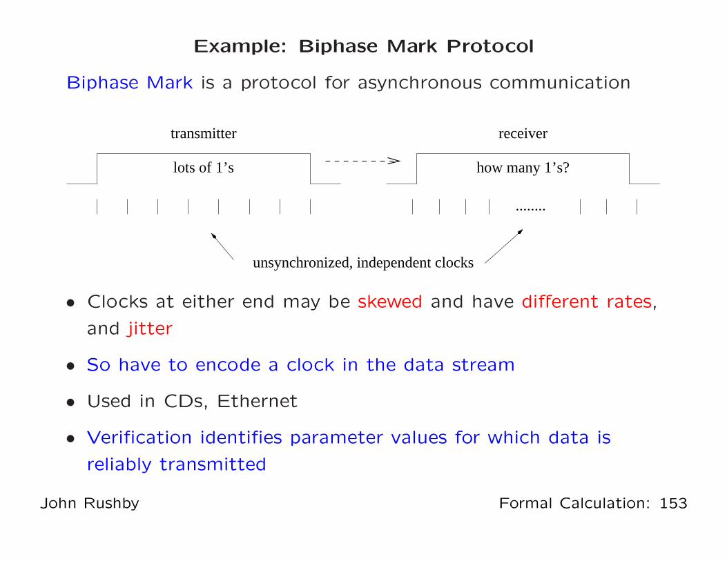
Example: Biphase Mark Protocol
Biphase Mark is a protocol for asynchronous communication
receiver
lots of 1’s how many 1’s?
........
unsynchronized, independent clocks
transmitter
• Clocks at either end may be skewed and have different rates,
and jitter
• So have to encode a clock in the data stream
• Used in CDs, Ethernet
• Verification identifies parameter values for which data is
reliably transmitted
John Rushby Formal Calculation: 153

Example: Biphase Mark Protocol (ctd)
• Flip the signal at the begining of every bit cell
• For a 1 bit, flip it in the middle, too
• For a 0 bit, leave it constant
BMP encoding
1 1 0 1 0 0 1 1 1 0 1 1
Original bitsream
Prove this works provided the sender and reciever clocks run at
similar rates
John Rushby Formal Calculation: 154
Biphase Mark Protocol Verification
• Verified by human-guided proof in ACL2 by J Moore (1994)
• Three different verifications used PVS
◦ One by Groote and Vaandrager used PVS + UPPAAL
required 37 invariants, 4,000 proof steps, hours of prover
time to check
◦ Also done by Dand Van Hung
John Rushby Formal Calculation: 155

Verification Systems vs. SMT-Based Model Checkers
PVS SAL
Backends SMT Solver
Actually, both kinds will coexist as part of the evidential tool
bus—another talk
John Rushby Formal Calculation: 156

Biphase Mark Protocol Verification (ctd)
• Brown and Pike recently did it with sal-inf-bmc
◦ Used timeout automata to model timed aspects
◦ Statement of theorem discovered systematically using
disjunctive invariants (7 disjuncts)
◦ Three lemmas proved automatically with 1-induction,
◦ Theorem proved automatically using 5-induction
◦ Verification takes seconds to check
• Adapted verification to 8-N-1 protocol (used in UARTs)
◦ Automated proofs more reusable than step-by-step ones
◦ Additional lemma proved with 13-induction
◦ Theorem proved with 3-induction (7 disjuncts)
◦ Revealed a bug in published application note
John Rushby Formal Calculation: 157
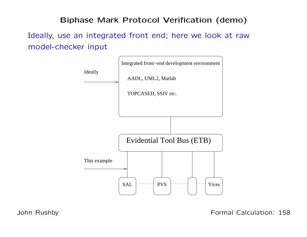
Biphase Mark Protocol Verification (demo)
Ideally, use an integrated front end; here we look at raw
model-checker input
This example
Evidential Tool Bus (ETB)
SAL PVS Yices
Integrated front−end development environment
AADL, UML2, Matlab
TOPCASED, SSIV etc.
Ideally
John Rushby Formal Calculation: 158

Summary
• The challenge faced by formal methods analysis tools is how
to search a huge space efficiently
• Theorem proving has developed efficient methods of local
search (decision procedures etc.)
• Model checking showed that efficient global search was
possible
• Now, methods are emerging that combine insights from both
approaches in a promising way
• And there a pragmatic focus on finding methods for using
the (still limited) capabilities of formal analysis tools to
address useful, but partial issues in big, real systems
• I have never felt more optimistic about the prospects for
formal analysis tools
John Rushby Formal Calculation: 159
Acknowledgments
• Very little of this is my work
• Most of it the work of my colleagues: Bruno Dutertre,
Leonardo de Moura, Sam Owre, Shankar, Ashish Tiwari
• With valuable contributions from Saddek Bensalem, Pavol
Cerny, Judy Crow, Jean-Christophe Filliatre, Klaus Havelund,
Friedrich von Henke, Yassine Lakhnech, Pat Lincoln, Cesar
Munoz, Holger Pfeifer, Lee Pike, Harald Rueß, Vlad Rusu,
Hassen Saıdi, Eli Singerman, Maria Sorea, Dave
Stringer-Calvert, Mike Whalen, and many others
John Rushby Formal Calculation: 160

To Learn More
• Check out papers and technical reports at
http://fm.csl.sri.com
• Information about PVS, and the system itself, is available
from http://pvs.csl.sri.com
◦ Version 4.0 is open source
◦ Built in Allegro and CMU Lisp for Linux, Mac
• Yices: http://yices.csl.sri.com
◦ Version 2.x is free binary
◦ Written in C
◦ Available as a library for C
• SAL: http://sal.csl.sri.com
◦ Version 2.4 is open source
◦ Written in Scheme, C++
John Rushby Formal Calculation: 161