Tutorial in Econometrics Part II: Sieve Inferences on Semi ... · PDF fileTutorial in...
66
Tutorial in Econometrics Part II: Sieve Inferences on Semi-nonparametric Models Xiaohong Chen (Yale) NUS, IMS, May 16, 2014 Chen () Tutorial in Econometrics Part II: Sieve Inferences on Semi-nonparametric Models NUS, IMS, May 16, 2014 1 / 42
Transcript of Tutorial in Econometrics Part II: Sieve Inferences on Semi ... · PDF fileTutorial in...
Tutorial in Econometrics Part II:Sieve Inferences on Semi-nonparametric Models
Xiaohong Chen (Yale)
NUS, IMS, May 16, 2014
Chen () Tutorial in Econometrics Part II: Sieve Inferences on Semi-nonparametric ModelsNUS, IMS, May 16, 2014 1 / 42
Outline of the Tutorial in Econometrics Part II
1 Introduction; Motivating empirical examples.2 Sieve extremum (M, MD, GMM...) estimation; Sieve two-step.3 Asymp. normality of sieve estimates.4 Sieve Wald statistic; sieve variance estimation.5 Sieve QLR statistics.6 Sieve F statistic for weakly dependent data.7 Concluding remarks.
Chen () Tutorial in Econometrics Part II: Sieve Inferences on Semi-nonparametric ModelsNUS, IMS, May 16, 2014 2 / 42
1. Introduction
Chen () Tutorial in Econometrics Part II: Sieve Inferences on Semi-nonparametric ModelsNUS, IMS, May 16, 2014 3 / 42
Introduction
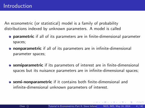
An econometric (or statistical) model is a family of probabilitydistributions indexed by unknown parameters. A model is called
parametric if all of its parameters are in �nite-dimensional parameterspaces;
nonparametric if all of its parameters are in in�nite-dimensionalparameter spaces;
semiparametric if its parameters of interest are in �nite-dimensionalspaces but its nuisance parameters are in in�nite-dimensional spaces;
semi-nonparametric if it contains both �nite-dimensional andin�nite-dimensional unknown parameters of interest.
Chen () Tutorial in Econometrics Part II: Sieve Inferences on Semi-nonparametric ModelsNUS, IMS, May 16, 2014 4 / 42
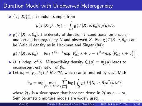
Duration Model with Unobserved Heterogeneity
fTi ,Xigni=1 a random sample from
p(T jX , β0, h0) =ZUg(T jX , u, β0)fU (u)du,
g(T jX , u, β0): the density of duration T conditional on a scalarunobserved heterogeneity U and observed X . Ex. g(T jX , u, β0) canbe Weibull density as in Heckman and Singer (84):
g(T jX , u, β0) = θ0,1T θ0,1�1 exphθ00,2X + u � T θ0,1 exp
�θ00,2X + u
�i.
U is indep. of X . Misspecifying density fU (u) � h20(u) leads toinconsistent estimation of θ0.Let α0 = (β0, h0) 2 B �H, which can estimated by sieve MLE:
bαn = arg maxβ2B , h2Hn
n
∑i=1logf
ZUg(Ti jXi , u, β)h2(u)dug
where Hn is a sieve space that becomes dense in H as n! ∞.Semiparametric mixture models are widely used.
Chen () Tutorial in Econometrics Part II: Sieve Inferences on Semi-nonparametric ModelsNUS, IMS, May 16, 2014 5 / 42
Shape-invariant system of Engel curves with endogenousexpenditure
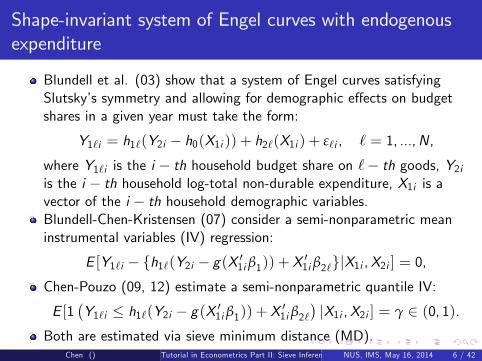
Blundell et al. (03) show that a system of Engel curves satisfyingSlutsky�s symmetry and allowing for demographic e¤ects on budgetshares in a given year must take the form:
Y1`i = h1`(Y2i � h0(X1i )) + h2`(X1i ) + ε`i , ` = 1, ...,N,
where Y1`i is the i � th household budget share on `� th goods, Y2iis the i � th household log-total non-durable expenditure, X1i is avector of the i � th household demographic variables.Blundell-Chen-Kristensen (07) consider a semi-nonparametric meaninstrumental variables (IV) regression:
E [Y1`i � fh1`(Y2i � g(X 01i β1)) + X 01i β2`gjX1i ,X2i ] = 0,Chen-Pouzo (09, 12) estimate a semi-nonparametric quantile IV:
E [1�Y1`i � h1`(Y2i � g(X 01i β1)) + X 01i β2`
�jX1i ,X2i ] = γ 2 (0, 1).
Both are estimated via sieve minimum distance (MD).Chen () Tutorial in Econometrics Part II: Sieve Inferences on Semi-nonparametric ModelsNUS, IMS, May 16, 2014 6 / 42
Nonlinear habit-based asset pricing models
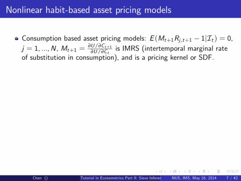
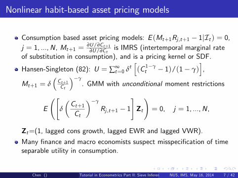
Consumption based asset pricing models: E (Mt+1Rj ,t+1 � 1jIt ) = 0,j = 1, ...,N, Mt+1 =
∂U/∂Ct+1∂U/∂Ct
is IMRS (intertemporal marginal rateof substitution in consumption), and is a pricing kernel or SDF.
Hansen-Singleton (82): U = ∑∞t=0 δt
h(C 1�γt � 1)/(1� γ)
i,
Mt+1 = δ�Ct+1Ct
��γ. GMM with unconditional moment restrictions
E
"δ
�Ct+1Ct
��γ
Rj ,t+1 � 1#Zt
!= 0, j = 1, ...,N,
Zt=(1, lagged cons growth, lagged EWR and lagged VWR).Many �nance and macro economists suspect misspeci�cation of timeseparable utility in consumption.
Chen () Tutorial in Econometrics Part II: Sieve Inferences on Semi-nonparametric ModelsNUS, IMS, May 16, 2014 7 / 42

Nonlinear habit-based asset pricing models
Consumption based asset pricing models: E (Mt+1Rj ,t+1 � 1jIt ) = 0,j = 1, ...,N, Mt+1 =
∂U/∂Ct+1∂U/∂Ct
is IMRS (intertemporal marginal rateof substitution in consumption), and is a pricing kernel or SDF.
Hansen-Singleton (82): U = ∑∞t=0 δt
h(C 1�γt � 1)/(1� γ)
i,
Mt+1 = δ�Ct+1Ct
��γ. GMM with unconditional moment restrictions
E
"δ
�Ct+1Ct
��γ
Rj ,t+1 � 1#Zt
!= 0, j = 1, ...,N,
Zt=(1, lagged cons growth, lagged EWR and lagged VWR).
Many �nance and macro economists suspect misspeci�cation of timeseparable utility in consumption.
Chen () Tutorial in Econometrics Part II: Sieve Inferences on Semi-nonparametric ModelsNUS, IMS, May 16, 2014 7 / 42
Nonlinear habit-based asset pricing models
Consumption based asset pricing models: E (Mt+1Rj ,t+1 � 1jIt ) = 0,j = 1, ...,N, Mt+1 =
∂U/∂Ct+1∂U/∂Ct
is IMRS (intertemporal marginal rateof substitution in consumption), and is a pricing kernel or SDF.
Hansen-Singleton (82): U = ∑∞t=0 δt
h(C 1�γt � 1)/(1� γ)
i,
Mt+1 = δ�Ct+1Ct
��γ. GMM with unconditional moment restrictions
E
"δ
�Ct+1Ct
��γ
Rj ,t+1 � 1#Zt
!= 0, j = 1, ...,N,
Zt=(1, lagged cons growth, lagged EWR and lagged VWR).Many �nance and macro economists suspect misspeci�cation of timeseparable utility in consumption.
Chen () Tutorial in Econometrics Part II: Sieve Inferences on Semi-nonparametric ModelsNUS, IMS, May 16, 2014 7 / 42
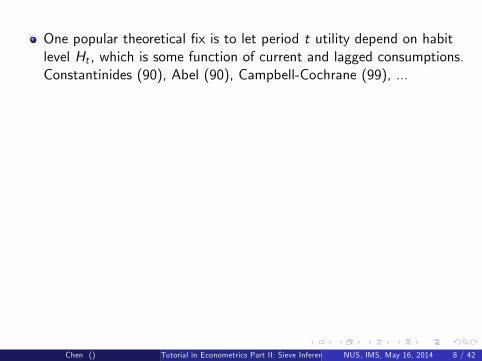
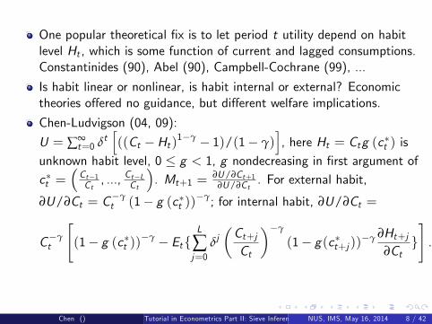
One popular theoretical �x is to let period t utility depend on habitlevel Ht , which is some function of current and lagged consumptions.Constantinides (90), Abel (90), Campbell-Cochrane (99), ...
Is habit linear or nonlinear, is habit internal or external? Economictheories o¤ered no guidance, but di¤erent welfare implications.
Chen-Ludvigson (04, 09):
U = ∑∞t=0 δt
h((Ct �Ht )1�γ � 1)/(1� γ)
i, here Ht = Ctg (c�t ) is
unknown habit level, 0 � g < 1, g nondecreasing in �rst argument ofc�t =
�Ct�1Ct, ..., Ct�LCt
�. Mt+1 =
∂U/∂Ct+1∂U/∂Ct
. For external habit,
∂U/∂Ct = C�γt (1� g (c�t ))
�γ; for internal habit, ∂U/∂Ct =
C�γt
"(1� g (c�t ))
�γ � EtfL
∑j=0
δj�Ct+jCt
��γ
(1� g(c�t+j ))�γ ∂Ht+j∂Ct
g#.
Chen () Tutorial in Econometrics Part II: Sieve Inferences on Semi-nonparametric ModelsNUS, IMS, May 16, 2014 8 / 42
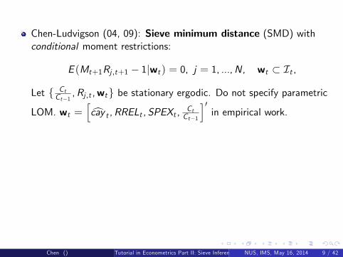
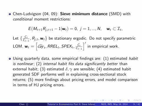
Chen-Ludvigson (04, 09): Sieve minimum distance (SMD) withconditional moment restrictions:
E (Mt+1Rj ,t+1 � 1jwt ) = 0, j = 1, ...,N, wt � It ,
Let f CtCt�1
,Rj ,t ,wtg be stationary ergodic. Do not specify parametric
LOM. wt =h ccay t ,RRELt ,SPEXt , Ct
Ct�1
i0in empirical work.
Using quarterly data, some empirical �ndings are: (1) estimated habitis nonlinear ; (2) internal habit �ts data signi�cantly better thanexternal habit; (3) estimated δ,γ are sensible; (4) estimated habitgenerated SDF performs well in explaining cross-sectional stockreturns; (5) more �ndings about pricing errors, and model comparisonin terms of HJ pricing errors.
Chen () Tutorial in Econometrics Part II: Sieve Inferences on Semi-nonparametric ModelsNUS, IMS, May 16, 2014 9 / 42
Semi-nonparametric GARCH + residual copula models
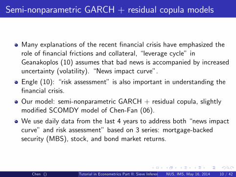
Many explanations of the recent �nancial crisis have emphasized therole of �nancial frictions and collateral, �leverage cycle� inGeanakoplos (10) assumes that bad news is accompanied by increaseduncertainty (volatility). �News impact curve�.
Engle (10): �risk assessment� is also important in understanding the�nancial crisis.
Our model: semi-nonparametric GARCH + residual copula, slightlymodi�ed SCOMDY model of Chen-Fan (06).
We use daily data from the last 4 years to address both �news impactcurve�and risk assessment�based on 3 series: mortgage-backedsecurity (MBS), stock, and bond market returns.
Chen () Tutorial in Econometrics Part II: Sieve Inferences on Semi-nonparametric ModelsNUS, IMS, May 16, 2014 10 / 42
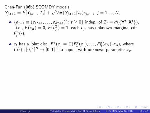
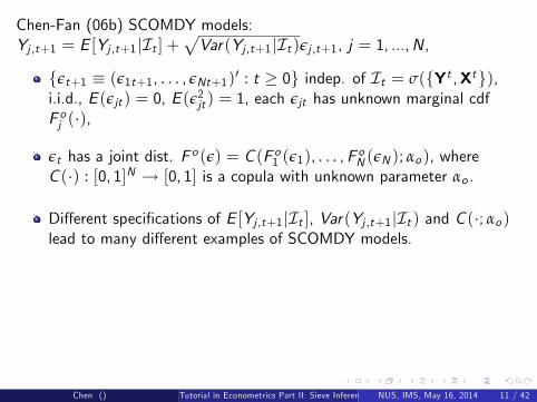
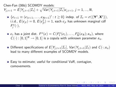
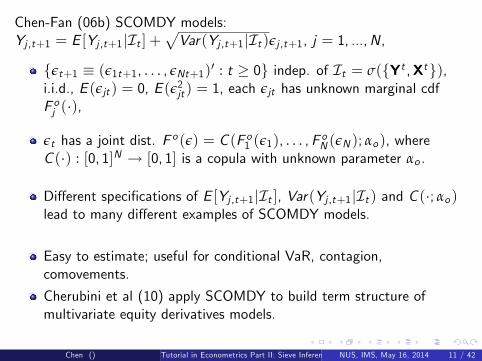
Chen-Fan (06b) SCOMDY models:Yj ,t+1 = E [Yj ,t+1jIt ] +
pVar(Yj ,t+1jIt )εj ,t+1, j = 1, ...,N,
fεt+1 � (ε1t+1, . . . , εNt+1)0 : t � 0g indep. of It = σ(fYt ,Xtg),i.i.d., E (εjt ) = 0, E (ε2jt ) = 1, each εjt has unknown marginal cdfF oj (�),
εt has a joint dist. F o (ε) = C (F o1 (ε1), . . . ,F oN (εN ); αo ), whereC (�) : [0, 1]N ! [0, 1] is a copula with unknown parameter αo .
Di¤erent speci�cations of E [Yj ,t+1jIt ], Var(Yj ,t+1jIt ) and C (�; αo )lead to many di¤erent examples of SCOMDY models.
Easy to estimate; useful for conditional VaR, contagion,comovements.
Cherubini et al (10) apply SCOMDY to build term structure ofmultivariate equity derivatives models.
Chen () Tutorial in Econometrics Part II: Sieve Inferences on Semi-nonparametric ModelsNUS, IMS, May 16, 2014 11 / 42
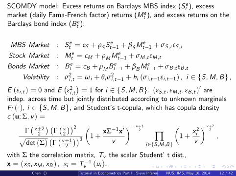
SCOMDY model: Excess returns on Barclays MBS index (Set ), excessmarket (daily Fama-French factor) returns (Me
t ), and excess returns on theBarclays bond index (Bet ):
MBS Market : Set = cS + ρSSet�1 + βSM
et�1 + σS ,t εS ,t
Stock Market : Met = cM + ρMM
et�1 + σM ,t εM ,t
Bonds Market : Bet = cB + ρMBet�1 + βBM
et�1 + σB ,t εB ,t
Volatility : σ2i ,t = ωi + θiσ2i ,t�1 + hi (σi ,t�1εi ,t�1) , i 2 fS ,M,Bg ,
E (εi ,t ) = 0 and E�ε2i ,t�= 1 for i 2 fS ,M,Bg. (εS ,t , εM ,t , εB ,t )0 are
indep. across time but jointly distributed according to unknown marginalsFi (�), i 2 fS ,M,Bg, and Student�s t-copula, which has copula densityc (u;Σ, v) =
Γ� v+2
2
� �Γ� v2
��2pdet (Σ)
�Γ� v+1
2
��3 �1+ x�1x0
v
�� v+32
∏i2fS ,M ,Bg
�1+
x2iv
� v+22
,
with Σ the correlation matrix, Tv the scalar Student�t dist.,x = (xS , xM , xB ) , xi = T�1v (ui ).
Chen () Tutorial in Econometrics Part II: Sieve Inferences on Semi-nonparametric ModelsNUS, IMS, May 16, 2014 12 / 42
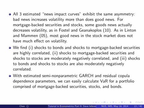
All 3 estimated �news impact curves� exhibit the same asymmetry:bad news increases volatility more than does good news. Formortgage-backed securities and stocks, some goods news actuallydecreases volatility, as in Fostel and Geanakoplos (10). As in Lintonand Mammen (05), most good news in the stock market does nothave much e¤ect on volatility.
We �nd (i) shocks to bonds and shocks to mortgage-backed securitiesare highly correlated, (ii) shocks to mortgage-backed securities andshocks to stocks are moderately negatively correlated, and (iii) shocksto bonds and shocks to stocks are also moderately negativelycorrelated.
With estimated semi-nonparametric GARCH and residual copuladependence parameters, we can easily calculate VaR for a portfoliocomprised of mortgage-backed securities, stocks, and bonds.
Chen () Tutorial in Econometrics Part II: Sieve Inferences on Semi-nonparametric ModelsNUS, IMS, May 16, 2014 13 / 42
2. Sieve Extremum Estimation
Chen () Tutorial in Econometrics Part II: Sieve Inferences on Semi-nonparametric ModelsNUS, IMS, May 16, 2014 14 / 42
Sieve extremum estimation
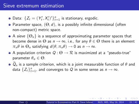
Data: fZt = (Y 0t ,X 0t )0gnt=1 is stationary, ergodic.
Parameter space, (Θ, d), is a possibly in�nite dimensional (oftennon-compact) metric space.
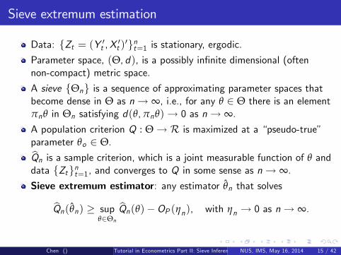
A sieve fΘng is a sequence of approximating parameter spaces thatbecome dense in Θ as n! ∞, i.e., for any θ 2 Θ there is an elementπnθ in Θn satisfying d(θ,πnθ)! 0 as n! ∞.A population criterion Q : Θ ! R is maximized at a �pseudo-true�parameter θo 2 Θ.bQn is a sample criterion, which is a joint measurable function of θ anddata fZtgnt=1, and converges to Q in some sense as n! ∞.Sieve extremum estimator: any estimator θ̂n that solves
bQn(θ̂n) � supθ2Θn
bQn(θ)�OP (ηn), with ηn ! 0 as n! ∞.
Chen () Tutorial in Econometrics Part II: Sieve Inferences on Semi-nonparametric ModelsNUS, IMS, May 16, 2014 15 / 42
Sieve extremum estimation
Data: fZt = (Y 0t ,X 0t )0gnt=1 is stationary, ergodic.Parameter space, (Θ, d), is a possibly in�nite dimensional (oftennon-compact) metric space.
A sieve fΘng is a sequence of approximating parameter spaces thatbecome dense in Θ as n! ∞, i.e., for any θ 2 Θ there is an elementπnθ in Θn satisfying d(θ,πnθ)! 0 as n! ∞.
A population criterion Q : Θ ! R is maximized at a �pseudo-true�parameter θo 2 Θ.bQn is a sample criterion, which is a joint measurable function of θ anddata fZtgnt=1, and converges to Q in some sense as n! ∞.Sieve extremum estimator: any estimator θ̂n that solves
bQn(θ̂n) � supθ2Θn
bQn(θ)�OP (ηn), with ηn ! 0 as n! ∞.
Chen () Tutorial in Econometrics Part II: Sieve Inferences on Semi-nonparametric ModelsNUS, IMS, May 16, 2014 15 / 42
Sieve extremum estimation
Data: fZt = (Y 0t ,X 0t )0gnt=1 is stationary, ergodic.Parameter space, (Θ, d), is a possibly in�nite dimensional (oftennon-compact) metric space.
A sieve fΘng is a sequence of approximating parameter spaces thatbecome dense in Θ as n! ∞, i.e., for any θ 2 Θ there is an elementπnθ in Θn satisfying d(θ,πnθ)! 0 as n! ∞.A population criterion Q : Θ ! R is maximized at a �pseudo-true�parameter θo 2 Θ.
bQn is a sample criterion, which is a joint measurable function of θ anddata fZtgnt=1, and converges to Q in some sense as n! ∞.Sieve extremum estimator: any estimator θ̂n that solves
bQn(θ̂n) � supθ2Θn
bQn(θ)�OP (ηn), with ηn ! 0 as n! ∞.
Chen () Tutorial in Econometrics Part II: Sieve Inferences on Semi-nonparametric ModelsNUS, IMS, May 16, 2014 15 / 42
Sieve extremum estimation
Data: fZt = (Y 0t ,X 0t )0gnt=1 is stationary, ergodic.Parameter space, (Θ, d), is a possibly in�nite dimensional (oftennon-compact) metric space.
A sieve fΘng is a sequence of approximating parameter spaces thatbecome dense in Θ as n! ∞, i.e., for any θ 2 Θ there is an elementπnθ in Θn satisfying d(θ,πnθ)! 0 as n! ∞.A population criterion Q : Θ ! R is maximized at a �pseudo-true�parameter θo 2 Θ.bQn is a sample criterion, which is a joint measurable function of θ anddata fZtgnt=1, and converges to Q in some sense as n! ∞.
Sieve extremum estimator: any estimator θ̂n that solves
bQn(θ̂n) � supθ2Θn
bQn(θ)�OP (ηn), with ηn ! 0 as n! ∞.
Chen () Tutorial in Econometrics Part II: Sieve Inferences on Semi-nonparametric ModelsNUS, IMS, May 16, 2014 15 / 42
Sieve extremum estimation
Data: fZt = (Y 0t ,X 0t )0gnt=1 is stationary, ergodic.Parameter space, (Θ, d), is a possibly in�nite dimensional (oftennon-compact) metric space.
A sieve fΘng is a sequence of approximating parameter spaces thatbecome dense in Θ as n! ∞, i.e., for any θ 2 Θ there is an elementπnθ in Θn satisfying d(θ,πnθ)! 0 as n! ∞.A population criterion Q : Θ ! R is maximized at a �pseudo-true�parameter θo 2 Θ.bQn is a sample criterion, which is a joint measurable function of θ anddata fZtgnt=1, and converges to Q in some sense as n! ∞.Sieve extremum estimator: any estimator θ̂n that solves
bQn(θ̂n) � supθ2Θn
bQn(θ)�OP (ηn), with ηn ! 0 as n! ∞.
Chen () Tutorial in Econometrics Part II: Sieve Inferences on Semi-nonparametric ModelsNUS, IMS, May 16, 2014 15 / 42
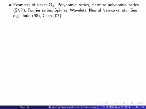
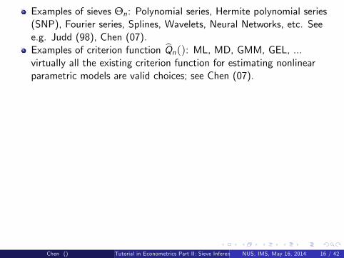
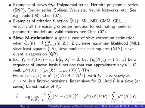
Examples of sieves Θn: Polynomial series, Hermite polynomial series(SNP), Fourier series, Splines, Wavelets, Neural Networks, etc. Seee.g. Judd (98), Chen (07).
Examples of criterion function bQn(): ML, MD, GMM, GEL, ...virtually all the existing criterion function for estimating nonlinearparametric models are valid choices; see Chen (07).Sieve M-estimation: a special case of sieve extremum estimationwhen bQn(θ) = 1
n ∑nt=1 l(θ,Zt ). E.g., sieve maximum likelihood (ML),
sieve least squares (LS), sieve nonlinear least squares (NLS), sievequantile regression (QR).Ex: Yt = θo (Xt ) + εt , E [εt jXt ] = 0. Let fpj (X ), j = 1, 2, ...g be asequence of known basis functions that can approximate any θ 2 Θwell. pkn (X ) = (p1(X ), ..., pkn (X ))
0. ThenΘn = fh : h(x) = pkn (x)0A : A 2 Rkng, with kn ! ∞ slowly asn! ∞, is a �nite-dimensional linear sieve for Θ. And bθ is a sieve (orseries) LS estimator of θo :
bθ = arg maxθ2Θn
�1n
n
∑t=1[Yt � θ(Xt )]2 = pkn (�)0(P 0P)�
n
∑t=1pkn (Xt )Yt .
Chen () Tutorial in Econometrics Part II: Sieve Inferences on Semi-nonparametric ModelsNUS, IMS, May 16, 2014 16 / 42
Examples of sieves Θn: Polynomial series, Hermite polynomial series(SNP), Fourier series, Splines, Wavelets, Neural Networks, etc. Seee.g. Judd (98), Chen (07).Examples of criterion function bQn(): ML, MD, GMM, GEL, ...virtually all the existing criterion function for estimating nonlinearparametric models are valid choices; see Chen (07).
Sieve M-estimation: a special case of sieve extremum estimationwhen bQn(θ) = 1
n ∑nt=1 l(θ,Zt ). E.g., sieve maximum likelihood (ML),
sieve least squares (LS), sieve nonlinear least squares (NLS), sievequantile regression (QR).Ex: Yt = θo (Xt ) + εt , E [εt jXt ] = 0. Let fpj (X ), j = 1, 2, ...g be asequence of known basis functions that can approximate any θ 2 Θwell. pkn (X ) = (p1(X ), ..., pkn (X ))
0. ThenΘn = fh : h(x) = pkn (x)0A : A 2 Rkng, with kn ! ∞ slowly asn! ∞, is a �nite-dimensional linear sieve for Θ. And bθ is a sieve (orseries) LS estimator of θo :
bθ = arg maxθ2Θn
�1n
n
∑t=1[Yt � θ(Xt )]2 = pkn (�)0(P 0P)�
n
∑t=1pkn (Xt )Yt .
Chen () Tutorial in Econometrics Part II: Sieve Inferences on Semi-nonparametric ModelsNUS, IMS, May 16, 2014 16 / 42

Examples of sieves Θn: Polynomial series, Hermite polynomial series(SNP), Fourier series, Splines, Wavelets, Neural Networks, etc. Seee.g. Judd (98), Chen (07).Examples of criterion function bQn(): ML, MD, GMM, GEL, ...virtually all the existing criterion function for estimating nonlinearparametric models are valid choices; see Chen (07).Sieve M-estimation: a special case of sieve extremum estimationwhen bQn(θ) = 1
n ∑nt=1 l(θ,Zt ). E.g., sieve maximum likelihood (ML),
sieve least squares (LS), sieve nonlinear least squares (NLS), sievequantile regression (QR).
Ex: Yt = θo (Xt ) + εt , E [εt jXt ] = 0. Let fpj (X ), j = 1, 2, ...g be asequence of known basis functions that can approximate any θ 2 Θwell. pkn (X ) = (p1(X ), ..., pkn (X ))
0. ThenΘn = fh : h(x) = pkn (x)0A : A 2 Rkng, with kn ! ∞ slowly asn! ∞, is a �nite-dimensional linear sieve for Θ. And bθ is a sieve (orseries) LS estimator of θo :
bθ = arg maxθ2Θn
�1n
n
∑t=1[Yt � θ(Xt )]2 = pkn (�)0(P 0P)�
n
∑t=1pkn (Xt )Yt .
Chen () Tutorial in Econometrics Part II: Sieve Inferences on Semi-nonparametric ModelsNUS, IMS, May 16, 2014 16 / 42
Examples of sieves Θn: Polynomial series, Hermite polynomial series(SNP), Fourier series, Splines, Wavelets, Neural Networks, etc. Seee.g. Judd (98), Chen (07).Examples of criterion function bQn(): ML, MD, GMM, GEL, ...virtually all the existing criterion function for estimating nonlinearparametric models are valid choices; see Chen (07).Sieve M-estimation: a special case of sieve extremum estimationwhen bQn(θ) = 1
n ∑nt=1 l(θ,Zt ). E.g., sieve maximum likelihood (ML),
sieve least squares (LS), sieve nonlinear least squares (NLS), sievequantile regression (QR).Ex: Yt = θo (Xt ) + εt , E [εt jXt ] = 0. Let fpj (X ), j = 1, 2, ...g be asequence of known basis functions that can approximate any θ 2 Θwell. pkn (X ) = (p1(X ), ..., pkn (X ))
0. ThenΘn = fh : h(x) = pkn (x)0A : A 2 Rkng, with kn ! ∞ slowly asn! ∞, is a �nite-dimensional linear sieve for Θ. And bθ is a sieve (orseries) LS estimator of θo :
bθ = arg maxθ2Θn
�1n
n
∑t=1[Yt � θ(Xt )]2 = pkn (�)0(P 0P)�
n
∑t=1pkn (Xt )Yt .
Chen () Tutorial in Econometrics Part II: Sieve Inferences on Semi-nonparametric ModelsNUS, IMS, May 16, 2014 16 / 42
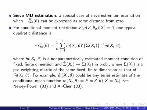
Sieve MD estimation: a special case of sieve extremum estimationwhen �bQn(θ) can be expressed as some distance from zero.
For conditional moment restriction E [ρ(Z , θo )jX ] = 0, one typicalquadratic distance is
�bQn(θ) = 1n
n
∑t=1
bm(Xt , θ)0fbΣ(Xt )g�1 bm(Xt , θ),where bm(Xt , θ) is a nonparametrically estimated moment condition of�xed, �nite dimension and bΣ(Xt )! Σ(Xt ) in prob., where Σ(Xt ) is apsd weighting matrix of the same �xed, �nite dimension as that ofbm(Xt , θ). For example, bm(Xt , θ) could be any series estimate of theconditional mean function m(Xt , θ) = E [ρ(Z , θ)jX = Xt ]; seeNewey-Powell (03) and Ai-Chen (03).
Chen () Tutorial in Econometrics Part II: Sieve Inferences on Semi-nonparametric ModelsNUS, IMS, May 16, 2014 17 / 42
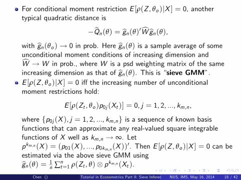
For conditional moment restriction E [ρ(Z , θo )jX ] = 0, anothertypical quadratic distance is
�bQn(θ) = bgn(θ)0cW bgn(θ),with bgn(θo )! 0 in prob. Here bgn(θ) is a sample average of someunconditional moment conditions of increasing dimension andcW ! W in prob., where W is a psd weighting matrix of the sameincreasing dimension as that of bgn(θ). This is �sieve GMM�.E [ρ(Z , θo )jX ] = 0 i¤ the increasing number of unconditionalmoment restrictions hold:
E [ρ(Zt , θo )p0j (Xt )] = 0, j = 1, 2, ..., km,n,
where fp0j (X ), j = 1, 2, ..., km,ng is a sequence of known basisfunctions that can approximate any real-valued square integrablefunctions of X well as km,n ! ∞. Letpkm,n (X ) = (p01(X ), ..., p0km,n (X ))
0. Then E [ρ(Z , θo )jX ] = 0 can beestimated via the above sieve GMM usingbgn(θ) = 1
n ∑nt=1 ρ(Zt , θ) pkm,n (Xt ).
Chen () Tutorial in Econometrics Part II: Sieve Inferences on Semi-nonparametric ModelsNUS, IMS, May 16, 2014 18 / 42
Why method of sieves?
1 Easy to compute. Once when the unknown functions areapproximated by �nite dimensional sieves, the implementation is thesame as any parametric nonlinear extremum estimation.
2 Easier to impose shape (monotonicity, concavity), additivity,non-negativity and other restrictions on unknown functions.
3 Can simultaneously obtain optimal convergence rates for unknownfunctions and root-n normality for regular functionals (such as �nitedimensional parameter); see Chen-Shen (98, sieve M estimation fortime series); Chen-Pouzo (09, sieve MD for iid)
Chen () Tutorial in Econometrics Part II: Sieve Inferences on Semi-nonparametric ModelsNUS, IMS, May 16, 2014 19 / 42
Estimation methods for unknown functionals
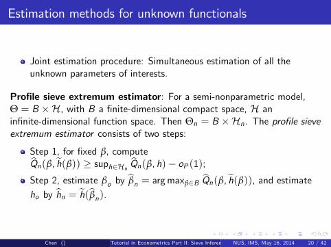
Joint estimation procedure: Simultaneous estimation of all theunknown parameters of interests.
Pro�le sieve extremum estimator: For a semi-nonparametric model,Θ = B �H, with B a �nite-dimensional compact space, H anin�nite-dimensional function space. Then Θn = B �Hn. The pro�le sieveextremum estimator consists of two steps:
Step 1, for �xed β, computebQn(β,eh(β)) � suph2Hn bQn(β, h)� oP (1);Step 2, estimate βo by bβn = argmaxβ2B bQn(β,eh(β)), and estimateho by bhn = eh(bβn).
Chen () Tutorial in Econometrics Part II: Sieve Inferences on Semi-nonparametric ModelsNUS, IMS, May 16, 2014 20 / 42
Estimation methods for unknown functionals
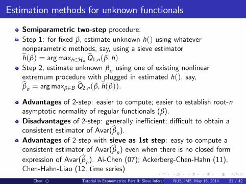
Semiparametric two-step procedure:Step 1: for �xed β, estimate unknown h() using whatevernonparametric methods, say, using a sieve estimatoreh(β) = argmaxh2Hn bQ1,n(β, h)Step 2, estimate unknown βo using one of existing nonlinearextremum procedure with plugged in estimated h(), say,bβn = argmaxβ2B bQ2,n(β,eh(β)).Advantages of 2-step: easier to compute; easier to establish root-nasymptotic normality of regular functionals (β).Disadvantages of 2-step: generally ine¢ cient; di¢ cult to obtain aconsistent estimator of Avar(bβn).Advantages of 2-step with sieve as 1st step: easy to compute aconsistent estimator of Avar(bβn) even when there is no closed formexpression of Avar(bβn). Ai-Chen (07); Ackerberg-Chen-Hahn (11),Chen-Hahn-Liao (12, time series)
Chen () Tutorial in Econometrics Part II: Sieve Inferences on Semi-nonparametric ModelsNUS, IMS, May 16, 2014 21 / 42
Example: Semi-nonparametric copula-based Markov model
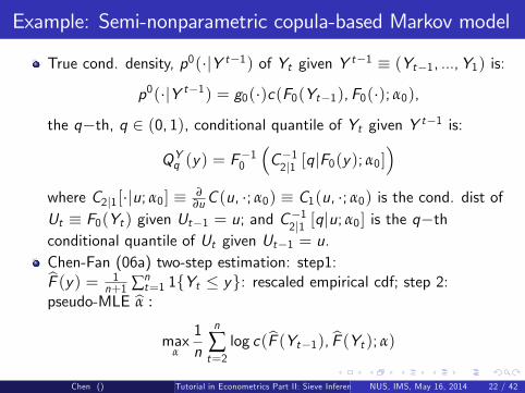
True cond. density, p0(�jY t�1) of Yt given Y t�1 � (Yt�1, ...,Y1) is:
p0(�jY t�1) = g0(�)c(F0(Yt�1),F0(�); α0),
the q�th, q 2 (0, 1), conditional quantile of Yt given Y t�1 is:
QYq (y) = F�10
�C�12j1 [qjF0(y); α0]
�where C2j1[�ju; α0] � ∂
∂uC (u, �; α0) � C1(u, �; α0) is the cond. dist ofUt � F0(Yt ) given Ut�1 = u; and C�12j1 [qju; α0] is the q�thconditional quantile of Ut given Ut�1 = u.Chen-Fan (06a) two-step estimation: step1:bF (y) = 1
n+1 ∑nt=1 1fYt � yg: rescaled empirical cdf; step 2:
pseudo-MLE bα :
maxα
1n
n
∑t=2log c(bF (Yt�1), bF (Yt ); α)
Chen () Tutorial in Econometrics Part II: Sieve Inferences on Semi-nonparametric ModelsNUS, IMS, May 16, 2014 22 / 42
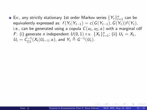
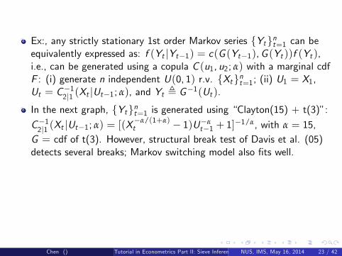
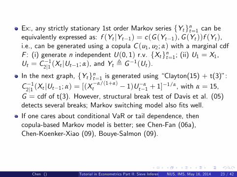
Ex:, any strictly stationary 1st order Markov series fYtgnt=1 can beequivalently expressed as: f (Yt jYt�1) = c(G (Yt�1),G (Yt ))f (Yt ),i.e., can be generated using a copula C (u1, u2; α) with a marginal cdfF : (i) generate n independent U(0, 1) r.v. fXtgnt=1; (ii) U1 = X1,Ut = C�12j1 (Xt jUt�1; α), and Yt , G�1(Ut ).
In the next graph, fYtgnt=1 is generated using �Clayton(15) + t(3)�:C�12j1 (Xt jUt�1; α) = [(X
�α/(1+α)t � 1)U�α
t�1 + 1]�1/α, with α = 15,
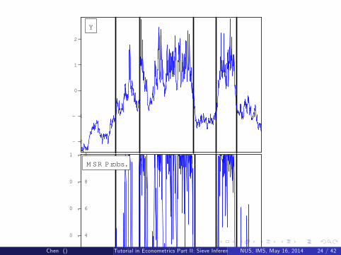
G = cdf of t(3). However, structural break test of Davis et al. (05)detects several breaks; Markov switching model also �ts well.
If one cares about conditional VaR or tail dependence, thencopula-based Markov model is better; see Chen-Fan (06a),Chen-Koenker-Xiao (09), Bouye-Salmon (09).
Chen () Tutorial in Econometrics Part II: Sieve Inferences on Semi-nonparametric ModelsNUS, IMS, May 16, 2014 23 / 42
Ex:, any strictly stationary 1st order Markov series fYtgnt=1 can beequivalently expressed as: f (Yt jYt�1) = c(G (Yt�1),G (Yt ))f (Yt ),i.e., can be generated using a copula C (u1, u2; α) with a marginal cdfF : (i) generate n independent U(0, 1) r.v. fXtgnt=1; (ii) U1 = X1,Ut = C�12j1 (Xt jUt�1; α), and Yt , G�1(Ut ).In the next graph, fYtgnt=1 is generated using �Clayton(15) + t(3)�:C�12j1 (Xt jUt�1; α) = [(X
�α/(1+α)t � 1)U�α
t�1 + 1]�1/α, with α = 15,
G = cdf of t(3). However, structural break test of Davis et al. (05)detects several breaks; Markov switching model also �ts well.
If one cares about conditional VaR or tail dependence, thencopula-based Markov model is better; see Chen-Fan (06a),Chen-Koenker-Xiao (09), Bouye-Salmon (09).
Chen () Tutorial in Econometrics Part II: Sieve Inferences on Semi-nonparametric ModelsNUS, IMS, May 16, 2014 23 / 42
2
1
0
1
2
0 . 0
0 . 2
0 . 4
0 . 6
0 . 8
1 . 0
1 0 02 0 03 0 04 0 05 0 06 0 07 0 08 0 09 0 01 0 0 0
M SR Probs.
Y
Chen () Tutorial in Econometrics Part II: Sieve Inferences on Semi-nonparametric ModelsNUS, IMS, May 16, 2014 24 / 42
Chen () Tutorial in Econometrics Part II: Sieve Inferences on Semi-nonparametric ModelsNUS, IMS, May 16, 2014 25 / 42
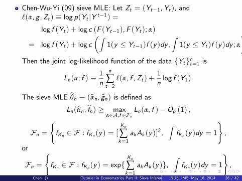
Chen-Wu-Yi (09) sieve MLE: Let Zt = (Yt�1,Yt ), and`(α, g ,Zt ) � log p(Yt jY t�1) =
log f (Yt ) + log c (F (Yt�1),F (Yt ); α)
= log f (Yt ) + log c�Z
1(y � Yt�1)f (y)dy ,Z1(y � Yt )f (y)dy ; α
�Then the joint log-likelihood function of the data fYtgnt=1 is
Ln(α, f ) �1n
n
∑t=2`(α, f ,Zt ) +
1nlog f (Y1).
The sieve MLE bθn � (bαn, bgn) is de�ned asLn(bαn,bfn) � max
α2A,f 2FnLn(α, f )�Op (1) ,
Fn =(fKn 2 F : fKn (y) = [
Kn
∑k=1
akAk (y)]2,ZfKn (y)dy = 1
),
or
Fn =(fKn 2 F : fKn (y) = expf
Kn
∑k=1
akAk (y)g,ZfKn (y)dy = 1
),
Chen () Tutorial in Econometrics Part II: Sieve Inferences on Semi-nonparametric ModelsNUS, IMS, May 16, 2014 26 / 42
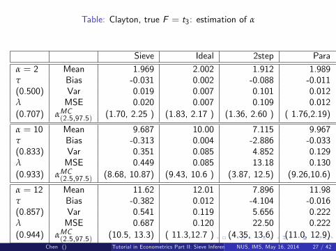
Table: Clayton, true F = t3: estimation of α
Sieve Ideal 2step Para Mis-N Mis-EVα = 2 Mean 1.969 2.002 1.912 1.989 2.400 2.957τ Bias -0.031 0.002 -0.088 -0.011 0.400 0.957(0.500) Var 0.019 0.007 0.101 0.012 0.103 0.056λ MSE 0.020 0.007 0.109 0.012 0.264 0.971(0.707) αMC(2.5,97.5) (1.70, 2.25 ) (1.83, 2.17 ) (1.36, 2.60 ) ( 1.76,2.19) (1.99,3.28) ( 2.57, 3.36 )
α = 10 Mean 9.687 10.00 7.115 9.967 11.42 11.57τ Bias -0.313 0.004 -2.886 -0.033 1.425 1.570(0.833) Var 0.351 0.085 4.852 0.129 0.577 1.194λ MSE 0.449 0.085 13.18 0.130 2.607 3.659(0.933) αMC(2.5,97.5) (8.68, 10.87) (9.43, 10.6 ) (3.87, 12.5) (9.26,10.6) ( 10.33,12.9) (9.68, 12.9)
α = 12 Mean 11.62 12.01 7.896 11.98 13.67 13.82τ Bias -0.382 0.012 -4.104 -0.016 1.668 1.816(0.857) Var 0.541 0.119 5.656 0.222 0.770 1.917λ MSE 0.687 0.120 22.50 0.222 3.552 5.214(0.944) αMC(2.5,97.5) (10.5, 13.3) ( 11.3,12.7 ) (4.35, 13.6) (11.0, 12.9) ( 12.3, 15.7) (11.4, 15.4)
Chen () Tutorial in Econometrics Part II: Sieve Inferences on Semi-nonparametric ModelsNUS, IMS, May 16, 2014 27 / 42
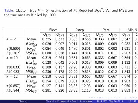
Table: Clayton, true F = t3: estimation of F . Reported Bias2, Var and MSE arethe true ones multiplied by 1000.
Sieve 2step Para Mis-N Mis-EVQ1/3 Q2/3 Q1/3 Q2/3 Q1/3 Q2/3 Q1/3 Q2/3 Q1/3 Q2/3
α = 2 Mean 0.325 0.673 0.333 0.666 0.333 0.667 0.347 0.557 0.382 0.614Bias2103 0.026 0.007 0.011 0.013 0.009 0.009 0.282 12.84 2.710 3.145
τ(0.500) Var103 0.054 0.049 1.430 0.801 0.002 0.002 1.921 5.651 0.755 0.947λ(0.707) MSE103 0.080 0.056 1.441 0.814 0.011 0.011 2.203 18.49 3.465 4.092α = 10 Mean 0.319 0.664 0.331 0.666 0.333 0.667 0.364 0.584 0.371 0.624
Bias2103 0.128 0.042 0.001 0.013 0.009 0.009 1.132 7.452 1.642 2.123τ(0.833) Var103 0.109 0.137 22.28 9.800 0.003 0.003 0.711 3.410 2.103 4.192λ(0.933) MSE103 0.236 0.178 22.29 9.813 0.012 0.012 1.843 10.86 3.744 6.315α = 12 Mean 0.318 0.661 0.331 0.665 0.333 0.667 0.374 0.598 0.375 0.633
Bias2103 0.154 0.079 0.001 0.023 0.010 0.010 1.903 5.242 2.052 1.351τ(0.857) Var103 0.127 0.141 28.83 12.08 0.003 0.003 0.950 2.662 2.494 4.934λ(0.944) MSE103 0.281 0.220 28.83 12.10 0.013 0.013 2.853 7.904 4.547 6.286
Chen () Tutorial in Econometrics Part II: Sieve Inferences on Semi-nonparametric ModelsNUS, IMS, May 16, 2014 28 / 42

Table: Clayton, true F = t3: estimation of 0.01 conditional quantile
Sieve Ideal 2step Para Mis-N Mis-EV
α = 5 IntBias2103 36.26 0.000 150.0 0.172 900.7 704.8τ(0.714) IntVar103 32.15 5.450 985.3 10.18 463.7 313.4λ(0.871) IntMSE103 68.41 5.450 1135 10.35 1364 1018
α = 10 IntBias2103 7.712 0.000 527.3 0.040 815.3 427.4τ(0.833) IntVar103 19.36 2.475 855.3 3.716 361.7 202.7λ(0.933) IntMSE103 27.07 2.475 1383 3.756 1177 630.1
α = 12 IntBias2103 2.851 0.000 367.7 0.004 181.1 175.9τ(0.857) IntVar103 6.236 1.068 590.9 1.578 59.44 46.12λ(0.944) IntMSE103 9.086 1.069 958.7 1.582 240.5 222.0
For each α, evaluation is based on the common support of 1000 MC simulateddata. Reported integrated Bias2, integrated Var and the integrated MSE are the
true ones multiplied by 1000.
Chen () Tutorial in Econometrics Part II: Sieve Inferences on Semi-nonparametric ModelsNUS, IMS, May 16, 2014 29 / 42
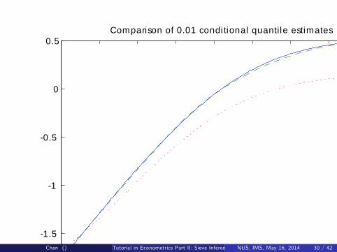
1.5 1 0.5 0 0.5 1 1.5 2 2.52
1.5
1
0.5
0
0.5Comparison of 0.01 conditional quantile estimates
true=solid, sieve=dashed, 2step=dotted
Chen () Tutorial in Econometrics Part II: Sieve Inferences on Semi-nonparametric ModelsNUS, IMS, May 16, 2014 30 / 42

3. Limiting distributions of sieve estimates.
Chen () Tutorial in Econometrics Part II: Sieve Inferences on Semi-nonparametric ModelsNUS, IMS, May 16, 2014 31 / 42

Limiting dist. of plug-in sieve estimates of regularfunctionals
pn normality of semiparametric 2-step GMM estimators: Newey
(94), Chen-Linton-Keilegom (03), Chen (07, beta-mixing, non-smoothcriterion).pn normality of sieve simultaneous M-estimator; e¢ ciency of sieve
MLE: Chen-Shen (98, beta-mixing)pn normality and inference of sieve MD estimator of
semi-nonparametric conditional moment restrictions: Ai-Chen (03,iid), Ai-Chen (07, could be misspeci�ed, iid), Chen-Pouzo (09, iid).
Chen () Tutorial in Econometrics Part II: Sieve Inferences on Semi-nonparametric ModelsNUS, IMS, May 16, 2014 32 / 42
Limiting dist. of plug-in sieve estimates of irregularfunctionals
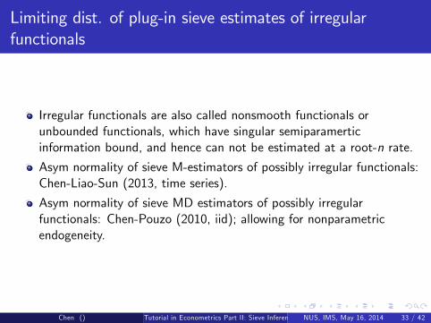
Irregular functionals are also called nonsmooth functionals orunbounded functionals, which have singular semiparamerticinformation bound, and hence can not be estimated at a root-n rate.
Asym normality of sieve M-estimators of possibly irregular functionals:Chen-Liao-Sun (2013, time series).
Asym normality of sieve MD estimators of possibly irregularfunctionals: Chen-Pouzo (2010, iid); allowing for nonparametricendogeneity.
Chen () Tutorial in Econometrics Part II: Sieve Inferences on Semi-nonparametric ModelsNUS, IMS, May 16, 2014 33 / 42
4. Sieve Wald statistics; consistent sieve varianceestimation.
Chen () Tutorial in Econometrics Part II: Sieve Inferences on Semi-nonparametric ModelsNUS, IMS, May 16, 2014 34 / 42
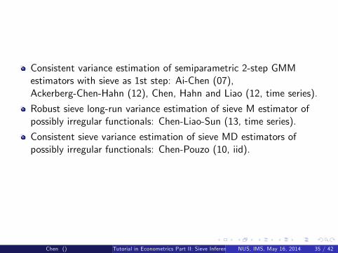
Consistent variance estimation of semiparametric 2-step GMMestimators with sieve as 1st step: Ai-Chen (07),Ackerberg-Chen-Hahn (12), Chen, Hahn and Liao (12, time series).
Robust sieve long-run variance estimation of sieve M estimator ofpossibly irregular functionals: Chen-Liao-Sun (13, time series).
Consistent sieve variance estimation of sieve MD estimators ofpossibly irregular functionals: Chen-Pouzo (10, iid).
Chen () Tutorial in Econometrics Part II: Sieve Inferences on Semi-nonparametric ModelsNUS, IMS, May 16, 2014 35 / 42
Sieve MD estimates of irregular functionals: Chen-Pouzo
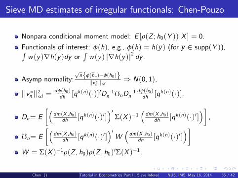
Nonpara conditional moment model: E [ρ(Z ; h0(Y ))jX ] = 0.Functionals of interest: φ(h), e.g., φ(h) = h(y) (for y 2 supp(Y )),Rw(y)rh(y)dy or
Rw(y) jrh(y)j2 dy .
Asymp normality:pnfφ(bhn)�φ(h0)g
jjv �n jjsd) N(0, 1),
jjv �n jj2sd =dφ(h0)dh [qk (n)(�)]0D�1n fnD�1n
dφ(h0)dh [qk (n)(�)],
Dn= E��
dm(X ,h0)dh [qk (n)(�)0]
�0Σ(X )�1
�dm(X ,h0)
dh [qk (n)(�)0]��,
fn= E��
dm(X ,h0)dh [qk (n)(�)0]
�0W�dm(X ,h0)
dh [qk (n)(�)0]��
W = Σ(X )�1ρ(Z , h0)ρ(Z , h0)0Σ(X )�1.
Chen () Tutorial in Econometrics Part II: Sieve Inferences on Semi-nonparametric ModelsNUS, IMS, May 16, 2014 36 / 42
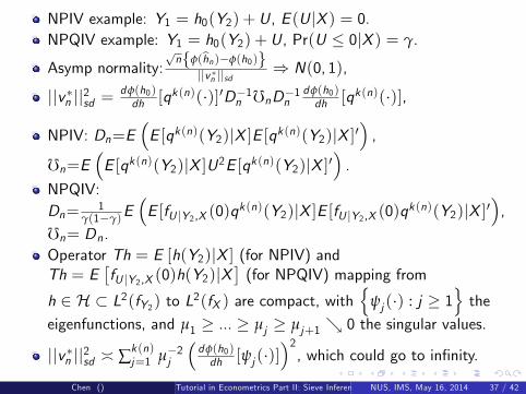
NPIV example: Y1 = h0(Y2) + U, E (U jX ) = 0.NPQIV example: Y1 = h0(Y2) + U, Pr(U � 0jX ) = γ.
Asymp normality:pnfφ(bhn)�φ(h0)g
jjv �n jjsd) N(0, 1),
jjv �n jj2sd =dφ(h0)dh [qk (n)(�)]0D�1n fnD�1n
dφ(h0)dh [qk (n)(�)],
NPIV: Dn=E�E [qk (n)(Y2)jX ]E [qk (n)(Y2)jX ]0
�,
fn=E�E [qk (n)(Y2)jX ]U2E [qk (n)(Y2)jX ]0
�.
NPQIV:Dn= 1
γ(1�γ)E�E [fU jY2,X (0)q
k (n)(Y2)jX ]E [fU jY2,X (0)qk (n)(Y2)jX ]0�,
fn= Dn.Operator Th = E [h(Y2)jX ] (for NPIV) andTh = E
�fU jY2,X (0)h(Y2)jX
�(for NPQIV) mapping from
h 2 H � L2(fY2) to L2(fX ) are compact, withn
ψj (�) : j � 1othe
eigenfunctions, and µ1 � ... � µj � µj+1 & 0 the singular values.
jjv �n jj2sd � ∑k (n)j=1 µ�2j
�dφ(h0)dh [ψj (�)]
�2, which could go to in�nity.
Chen () Tutorial in Econometrics Part II: Sieve Inferences on Semi-nonparametric ModelsNUS, IMS, May 16, 2014 37 / 42
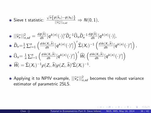
Sieve t statistic:pnfφ(bhn)�φ(h0)g
jjbv �n jjn,sd ) N(0, 1),
jjbv �n jj2n,sd = dφ(bh)dh [q
k (n)(�)]0 bD�1n bfn bD�1n dφ(bh)dh [q
k (n)(�)],
bDn= 1n ∑n
i=1
�d bm(Xi ,bh)
dh [qk (n)(�)0]�0 bΣ(Xi )�1 � d bm(Xi ,bh)dh [qk (n)(�)0]
�,
bfn= 1n ∑n
i=1
�d bm(Xi ,bh)
dh [qk (n)(�)0]�0cWi
�d bm(Xi ,bh)
dh [qk (n)(�)0]�
cWi = bΣ(Xi )�1ρ(Zi ,bh)ρ(Zi ,bh)0bΣ(Xi )�1.Applying it to NPIV example, jjbv �n jj2n,sd becomes the robust varianceestimator of parametric 2SLS.
Chen () Tutorial in Econometrics Part II: Sieve Inferences on Semi-nonparametric ModelsNUS, IMS, May 16, 2014 38 / 42
5. Sieve QLR statistics.
6. Sieve F statistic for weakly dependent data.
Chen () Tutorial in Econometrics Part II: Sieve Inferences on Semi-nonparametric ModelsNUS, IMS, May 16, 2014 39 / 42
7. Conclusion and future research
Chen () Tutorial in Econometrics Part II: Sieve Inferences on Semi-nonparametric ModelsNUS, IMS, May 16, 2014 40 / 42
Concluding remarks
Semi-nonparametric methods are useful for complicated nonlinearnon-Gaussian, nonseparable structural models.
Multi-step estimation is typical for complicated dynamic models.
Large sample properties (consistency, rate, limiting distribution) ofsieve M-estimation for weakly dependent time series models arerelatively complete; sieve Wald, QLR tests are also available and easyto implement
Large sample properties (consistency, rate, limiting distribution) ofsieve MD-estimation (or sieve GMM) for cross-section and small-Tpanel data structural models are relatively complete.
Sieve Wald, score and QLR tests, and their bootstrap versions basedon sieve MD for possible irregular functionals are developed.(Chen-Pouzo, 2013). This allows for inference on general class ofsemi-nonparametric conditional moment models involvingnonparametric endogeneity.
Chen () Tutorial in Econometrics Part II: Sieve Inferences on Semi-nonparametric ModelsNUS, IMS, May 16, 2014 41 / 42
Concluding remarks, future research
There is few result on higher order re�nements.
There is few result on simulation based methods forsemi-nonparametric time series models with nonlinear non-Gaussianlatent structures.
Choice of smoothing parameters and lag length.
Chen () Tutorial in Econometrics Part II: Sieve Inferences on Semi-nonparametric ModelsNUS, IMS, May 16, 2014 42 / 42