Tutorial — ICTAC 2004 Functional Predicate Calculus and ... · Functional Predicate Calculus and...

Tutorial — ICTAC 2004

Functional Predicate Calculus and Generic Functionals

in Software Engineering

Raymond Boute INTEC — Ghent University

13:30–13:40 0. Introduction: purpose and approach

13:40–14:30 Lecture A: Mathematical preliminaries and generic functionals1. Preliminaries: formal calculation with equality, propositions, sets

2. Functions and introduction to concrete generic functionals

14:30–15:00 (Half-hour break)

15:00–15:55 Lecture B: Functional predicate calculus; general applications

3. Functional predicate calculus: calculating with quantifiers4. General applications to functions, functionals, relations, induction

15:55–16:05 (Ten-minute break)

16:05–17:00 Lecture C: Applications in computer and software engineering

5. Applications of generic functionals in computing science6. Applications of formal calculation in programming theories

(given time) 7. Formal calculation as unification with classical engineering

0

Next topic


Lecture A: Mathematical preliminaries and generic functionals13:40–14:10 1. Preliminaries: formal calculation with equality, propositions, sets

14:10–14:30 2. Functions and introduction to concrete generic functionals

14:30–15:00 Half hour break

Lecture B: Functional predicate calculus and general applications

15:00–15:30 3. Functional predicate calculus: calculating with quantifiers15:30–15:55 4. General applications to functions, functionals, relations, induction

15:55–16:05 Ten-minute break

Lecture C: Applications in computer and software engineering

16:05–16:40 5. Applications of generic functionals in computing science16:40–17:00 6. Applications of formal calculation in programming theories


Note: depending on the definitive program for tutorials, times indicated may shift.

1

0 Introduction: Purpose and Approach

0.0 Purpose: strengthening link between theoretical CS and Engineering

0.1 Principle: formal calculation

0.2 Realization of the goal: Functional Mathematics (Funmath)

0.3 What you can get out of this

2

0.0 Purpose: strengthening link between theoretical CS and Engineering

• Remark by Parnas:

Professional engineers can often be distinguished from other designers by the engi-

neers’ ability to use mathematical models to describe and analyze their products.

• Observation: difference in practice

– In classical engineering (electrical, mechanical, civil): established de facto

– In software “engineering”: mathematical models rarely used

(occasionally in critical systems under the name “Formal Methods”)

C. Michael Holloway: [software designers want to be(come) engineers]

• Causes

– Different degree of preparation,

– Divergent mathematical methodology and style

3

• Methodology rift mirrors style breach throughout mathematics

– In long-standing areas of mathematics (algebra, analysis, etc.):

style of calculation essentially formal (“letting symbols do the work”)

Examples:

From: Blahut / data compacting

1

n

∑

x

pn(x|θ)ln(x)

≤ 1

n

∑

x

pn(x|θ)[1− log qn(x)]

=1

n+

1

nL(pn;qn) + Hn(θ)

=1

n+

1

nd(pn,G) + Hn(θ)

≤ 2

n+ Hn(θ)

From: Bracewell / transforms

F (s) =

∫ +∞

−∞e−|x|e−i2πxsdx

= 2

∫ +∞

0

e−x cos 2πxs dx

= 2 Re

∫ +∞

0

e−xei2πxsdx

= 2 Re−1

i2πs− 1

=2

4π2s2 + 1.

4

– Major defect: supporting logical arguments highly informal

“The notation of elementary school arithmetic, which nowadays everyone

takes for granted, took centuries to develop. There was an intermediatestage called syncopation, using abbreviations for the words for addition,

square, root, etc. For example Rafael Bombelli (c. 1560) would write

R. c. L. 2 p. di m. 11 L for our 3√

2 + 11i.

Many professional mathematicians to this day use the quantifiers (∀,∃)in a similar fashion,

∃δ > 0 s.t. |f(x)− f(x0)| < ǫ if |x− x0| < δ, for all ǫ > 0,

in spite of the efforts of [Frege, Peano, Russell] [. . .]. Even now, mathe-matics students are expected to learn complicated (ǫ-δ)-proofs in analy-

sis with no help in understanding the logical structure of the arguments.Examiners fully deserve the garbage that they get in return.”

(P. Taylor, “Practical Foundations of Mathematics”)

– Similar situation in Computing Science: even in formal areas (semantics),

style of theory development is similar to analysis texts.

5

0.1 Principle: formal calculation

• Mathematical styles

– “formal” = manipulating expressions on the basis of their form

– “informal” = manipulating expressions on the basis of their meaning

• Advantages of formality

– Usual arguments: precision, reliability of design etc. well-known

– Equally (or more) important: guidance in expression manipulation

Calculations guided by the shape of the formulas

UT FACIANT OPUS SIGNA(Maxim of the conferences on Mathematics of Program Construction)

• Ultimate goal: making formal calculation as elegant and practical for logic andcomputer engineering as shown by calculus and algebra for classical engineering

6

Goal has been achieved (illustration; calculation rules introduced later)

Proposition 2.1. for any function f : R→/ R, any subset S of D f and any

a adherent to S, (i) ∃ (L : R . L islimf a)⇒ ∃ (L : R . L islimf ⌉S a),(ii) ∀L : R . ∀M : R . L islimf a ∧M islimf ⌉S a⇒ L = M .

Proof for (ii): Letting b R δ abbreviate ∀x : S . |x− a| < δ ⇒ |f x− b| < ǫ,

L islimf a ∧M islimf ⌉S a

⇒ 〈Hint in proof for (i)〉 L islimf ⌉S a ∧M islimf ⌉S a

≡ 〈Def. islim, hypoth.〉 ∀ (ǫ : R>0 . ∃ δ : R>0 . L R δ) ∧ ∀ (ǫ : R>0 . ∃ δ : R>0 . M R δ)

≡ 〈Distributivity ∀/∧〉 ∀ ǫ : R>0 . ∃ (δ : R>0 . L R δ) ∧ ∃ (δ : R>0 . M R δ)

≡ 〈Rename, dstr. ∧/∃〉 ∀ ǫ : R>0 . ∃ δ : R>0 . ∃ δ′ : R>0 . L R δ ∧M R δ′

⇒ 〈Closeness lemma〉 ∀ ǫ : R>0 . ∃ δ : R>0 . ∃ δ′ : R>0 . a ∈ Ad S ⇒ |L−M | < 2 · ǫ≡ 〈Hypoth. a ∈ Ad S〉 ∀ ǫ : R>0 . ∃ δ : R>0 . ∃ δ′ : R>0 . |L−M | < 2 · ǫ≡ 〈Const. pred. sub ∃〉 ∀ ǫ : R>0 . |L−M | < 2 · ǫ≡ 〈Vanishing lemma〉 L−M = 0

≡ 〈Leibniz, group +〉 L = M

7

0.2 Realization of the goal: Functional Mathematics (Funmath)

• Unifying formalism for continuous and discrete mathematics

– Formalism = notation (language) + formal manipulation rules

• Characteristics

– Principle: functions as first-class objects and basis for unification

– Language: very simple (4 constructs only)

Synthesizes common notations, without their defects

Synthesizes new useful forms of expression, in particular: “point-free”,

e.g. square = times ◦ duplicate versus square x = x times x

– Formal rules: calculational

Why not use “of the shelf” (existing) mathematical conventions?

Answer: too many defects prohibit design of formal calculation rules.

8

• Remark: the need for defect-free notation

Examples of defects in common mathematical conventions

Examples A: defects in often-used conventions relevant to systems theory

– Ellipsis, i.e., dots (. . .) as in a0 + a1 + · · ·+ an

Common use violates Leibniz’s principle (substitution of equals for equals)

Example: ai = i2 and n = 7 yields 0+1+· · ·+49 (probably not intended!)

– Summation sign∑

not as well-understood as often assumed.

Example: error in Mathematica:∑n

i=1

∑mj=i 1 = n·(2·m−n+1)

2

Taking n := 3 and m := 1 yields 0 instead of the correct sum 1.

– Confusing function application with the function itself

Example: y(t) = x(t) ∗ h(t) where ∗ is convolution.

Causes incorrect instantiation, e.g., y(t− τ) = x(t− τ) ∗ h(t− τ)

9

Examples B: ambiguities in conventions for sets

– Patterns typical in mathematical writing:

(assuming logical expression p, arbitrary expression p

Patterns {x ∈ X | p} and {e | x ∈ X}Examples {m ∈ Z | m < n} and {n ·m | m ∈ Z}

The usual tacit convention is that ∈ binds x. This seems innocuous, BUT

– Ambiguity is revealed in case p or e is itself of the form y ∈ Y .

Example: let Even := {2 ·m | m ∈ Z} in

Patterns {x ∈ X | p} and {e | x ∈ X}Examples {n ∈ Z | n ∈ Even} and {n ∈ Even | n ∈ Z}

Both examples match both patterns, thereby illustrating the ambiguity.

– Worse: such defects prohibit even the formulation of calculation rules!

Formal calculation with set expressions rare/nonexistent in the literature.

Underlying cause: overloading relational operator ∈ for binding of a dummy.This poor convention is ubiquitous (not only for sets), as in ∀x ∈ R . x2 ≥ 0.

10

0.3 What you can get out of this

(As for all mathematics: with regular practice)

• Ability to calculate with quantifiers as smoothly as usually done with derivatives

and integrals

Note: the same for functionals, pointwise and point-free expressions

• Easier to explore new areas through formalization. Two steps:

– Formalize concepts using defect-free notation

– Use formal reasoning to assist “common” intuition

• Also for better understanding other people’s work (literature, other sources):formalize while removing defects, use formal calculation for exploration.

– Traditional student’s way: staring at a formula until understanding dawns(if ever)

– Calculational way: start formal calculation with the formula to “get a feel”

11

Next topic


Lecture A: Mathematical preliminaries and generic functionals

13:40–14:10 1. Preliminaries: formal calculation with equality, propositions, sets










12

1 Formal calculation with equality, propositions, sets

1.0 Simple expressions and equality

1.0.0 Syntax of simple expressions and equational formulas

1.0.1 Substitution and formal calculation with equality

1.1 Pointwise and point-free styles

1.1.0 Lambda calculus as a consistent method for handling dummies

1.1.1 Combinator calculus as an archetype for point-free formalisms

1.2 Calculational proposition logic and binary algebra

1.2.0 Syntax, conventions and calculational logic with implication and negation

1.2.1 Quick calculation rules and proof techniques; rules for derived operators

1.2.2 Binary Algebra and formal calculation with conditional expressions

1.3 Formal calculation with sets via proposition calculus

13

1.0 Simple expressions and equality

1.0.0 Syntax of simple expressions and equational formulas

a. Syntax of simple expressions Convention: terminal symbols underscored

expression ::= variable | constant0 | applicationapplication ::= (cop1 expression) | (expression cop2 expression)

Variables and constants are domain-dependent. Example (arithmetic):

variable ::= x | y | z cop1 ::= succ | predconstant0 ::= a | b | c cop2 ::= + | ·

Alternative style (Observe the conventions, e.g., variable is a nonterminal, V

its syntactic category, v an element of V , mostly using the same initial letter)

Ev: [[v]] where v is a variable from VE0: [[c]] where c is a constant from C0

E1: [[(φ e)]] where φ is an operator from C1 and e an expressionE2: [[(e ⋆ e′)]] where ⋆ is an operator from C2 and e and e′ expressions

14

b. Syntax of equational formulas [and a sneak preview of semantics]

formula ::= expression = expression

A sneak preview of semantics

• Informal

What does x + y mean? This clearly depends on x and y.

What does x + y = y + x mean? Usually the commutativity of +.

• Formal: later exercise

• For the time being: IGNORE semantics

We calculate FORMALLY, that is: without thinking about meaning!

The CALCULATION RULES obviate relying on meaning aspects.

15

1.0.1 Substitution and formal calculation with equality

a. Formalizing substitution

We define a “postfix” operator [v := d] (written after its argument),parametrized by variable v and expression d,

Purpose: e[v := d] is the result of substituting d for w in e.

We formalize this by recursion on the structure of the argument expression.

ref. image definition for [v := d] for arbitrary

Sv: w[v := d] = (v = w) ? d [[w]] variable w in VS0: c[v := d] = [[c]] constant c in C0

S1: (φ e)[v := d] = [[(φ e[v := d])]] φ in C1 and e in ES2: (e ⋆ e′)[v := d] = [[(e[v := d] ⋆ e′[v := d])]] ⋆ :C2, e :E and e′ : E

Legend for conditionals c ? b a (“if c then b else a”) is c ? e1 e0 = ec.

Remarks

• Straightforward extension to simultaneous substitution: [v′, v′′ := d′, d′′]

• Convention: often we write [vd for [v := d] (saves horizontal space).

16

b. Example (detailed calculation)

(a · succ x + y)[x := z · b]= 〈Normalize〉 ‘((a · (succ x)) + y)’[x := (z · b)]= 〈Rule S2〉 [[((a · (succ x))[x := (z · b)] + y[x := (z · b)])]]= 〈Rule S2〉 [[((a[x := (z · b)] · (succ x)[x := (z · b)]) + y[x := (z · b)])]]= 〈Rule S1〉 [[((a[x := (z · b)] · (succ x[x := (z · b)])) + y[x := (z · b)])]]= 〈Rule S0〉 [[((a · (succ x[x := (z · b)])) + y[x := (z · b)])]]= 〈Rule SV〉 ‘((a · (succ (z · b))) + y)’

= 〈Opt. par.〉 ‘a · succ (z · b) + y’

Observe how the rules (repeated below) distribute s over the variables.

ref. image definition for [v := d] for arbitrary

Sv: w[v := d] = (v = w) ? d [[w]] variable w in V

S0: c[v := d] = [[c]] constant c in C0

S1: (φ e)[v := d] = [[(φ e[v := d])]] φ in C1 and e in E

S2: (e ⋆ e′)[v := d] = [[(e[v := d] ⋆ e′[v := d])]] ⋆ :C2, e :E and e′ : E

17

c. Formal deduction: general

• An inference rule is a little table of the form

Premsq

where Prems is a collection of formulas (the premisses)

and q is a formula (the conclusion or direct consequence).

• It is used as follows. Given a collection Hpths (the hypotheses).Then a formula q is a consequence of Hpths, written

Hpths |− q,

in case

– either q is a formula in the collection Hpths

– or q is the conclusion of an inference rule where the premisses areconsequences of Hpths

An axiom is a hypothesis expressly designated as such (i.e., as an axiom).A theorem is a consequence of hypotheses that are axioms exclusively.

(Note: axioms are chosen s. t. they are valid in some useful context.)

18

d. Deduction with equality

The inference rules for equality are:

0. Instantiation (strict):p

p[v := e](α)

1. Leibniz’s principle (non-strict): d′ = d′′e[v := d′] = e[v := d′′]

(β)

2. Symmetry of equality (non-strict): e = e′e′ = e

(γ)

3. Transitivity of equality (non-strict):e = e′, e′ = e′′

e = e′′(δ)

Remarks

• An inference rule is strict if all of its premises must be theorems.Example: instantiating the axiom x · y = y · x with [x, y := (a + b), −b]

• Reflexivity of = is captured by Leibniz (if v does not occur in e).

19

e. Equational calculation: embedding the inference rules into the format

e0 = 〈justification0〉 e1

= 〈justification1〉 e1 and so on.

Using an inference rule with single premiss p and conclusion e′ = e′′ is written

e′ = 〈p〉 e′′, capturing each of the inference rules as follows.

(α) Instantiation Premiss p is a theorem of the form d′ = d′′, and hence the

conclusion p[v := e] is d′[v := e] = d′′[v := e] which has the form e′ = e′′.Example: (a + b) · −b =〈x · y = y · x〉 −b · (a + b).

(β) Leibniz Premiss p, not necessarily a theorem, is of the form d′ = d′′ and

the conclusion e[v := d′] = e[v := d′′] is of the form e′ = e′′.Example: if y = a · x, then we may write x + y =〈y = a · x〉 x + a · x.

(γ) Symmetry Premiss p, not necessarily a theorem, is of the form e′′ = e′.However, this simple step is usually taken tacitly.

(δ) Transitivity has two equalities for premisses. It is used implicitly to justify

chaining e0 = e1 and e1 = e2 in the format shown to conclude e0 = e2.

20

1.1 Pointwise and point-free styles

1.1.0 Lambda calculus as a consistent method for handling dummies

a. Syntax of “pure” lambda terms

• Syntax: the expressions are (lambda) terms, defined by

term ::= variable | (term term) | (λvariable.term)

We write Λ for the syntactic category. Metavariables: L ..R for terms, u,

v, w for variables. Shorthands for certain ”useful” terms: C, D, I etc,.

• Conventions for making certain parentheses and dots optional

– Optional: outer parentheses in (MN), and in (λv.M) if standing by

itself or as an abstrahend, e.g., λv.MN for λv.(MN), not (λv.M)N .

– Application “associates to the left”, e.g., (LMN) stands for ((LM)N).

– Nested abstractions may be merged by writing λu.λv.M as λuv.M .

So λx.y(λxy.xz(λz.xyz))yz is (λx.(((y(λx.(λy.((xz)(λz.((xy)z))))))y)z)).

• A form (MN) is an application and (λv.M) an abstraction. In (λv.M),

the λv. is the abstractor and M the abstrahend or the scope of λv.

21

b. Bound and free variables

• Definitions

Every occurrence of v in λv.M is called bound.

Occurrences that are not bound are called free.

A term without free variables is a closed term or a (lambda-)combinator.

Bound variables are also called dummies.

• Examples

(i) In λx.y(λxy.xz(λz.xyz))yz, number all occurrences from 0 to 11.

Only free occurrences: those of y and z in positions 1, 5, 10, 11.

(ii) An operator ϕ for the set of variables that occur free in a term:

ϕ [[v]] = ι v ϕ [[(MN)]] = ϕ M ∪ ϕN ϕ [[(λv.M)]] = (ϕ M) \ (ι v)

Legend: ι for singleton sets, ∪ for set union, \ for set difference.

(iii) Typical (and important) combinators are λxyz.x(yz) and λxyz.xzy

and λx.(λy.x(yy))(λy.x(yy)), abbreviated C, T, Y respectively.

22

c. Axioms and substitution rules

• Idea: ensure correct generalization of (λv.e) d = e[v := d], i.e.,

Axiom, β-conversion: (λv.M) N = M [v := N ]

This requires defining M [v := N ] for lambda terms.

• Avoiding name clashes inherent in naıve substitution, as in

((λx.(λy.xy))y)x = 〈β-convers.〉 ((λy.xy)[x := y])x= 〈Naıve subst.〉 (λy.yy)x (wrong!)

Avoidance principle: choice of dummy names is incidental.

• Resulting substitution rules

Svar: v[wL = (v = w) ? L [[v]]Sapp: (MN)[wL = (M [wL N [wL)

Sabs: (λv.M)[wL = (λu.M [vu[wL) (new u)

Variant: (λv.M)[wL= (v = w) ? (λv.M) (v 6∈ ϕ L) ? (λv.M [wL) (λu.M [vu[wL),

Checks for name clashes; if there are none, taking new u is unnecessary.

23

d. Calculation rules and axiom variants

• The rules of equality: symmetry, transitivity and Leibniz’s principle:

M = NN = M

L = M M = NL = N

M = NL[v := M ] = L[v := N ]

• The proper axioms common to most variants of the lambda calculus

Axiom, β-conversion: (λv.M)N = M [vNAxiom, α-conversion: (λv.M) = (λw.M [vw) provided w 6∈ ϕ M

Certain authors consider α-conversion subsumed by syntactic equality.

• Specific additional axioms characterizing variants of the lambda calculus.

(i) Rule ξ: M = Nλv.M = λv.N

(note: extends Leibniz’s principle)

(ii) Rule η (or η-conversion): (λv.Mv) = M provided v 6∈ ϕ M

(iii) Rule ζ (or extensionality): Mv = NvM = N provided v 6∈ ϕ (M, N)

Note: given the basic rules, rule ζ is equivalent to ξ and η combined.

Henceforth we assume all these rules.

24

e. Redexes and the Church-Rosser property

• Redexes

– A β-redex is a term of the form (λv.M)N . Example: (λxy.yx)(λx.y)

– A η-redex is a term of the form λv.Mv (met v 6∈ ϕ M).

– Warning example: λx.x(λy.y)x contains no redex.

• Normal forms

– A βη-normal form (or normal form) is a term containing no redex.

– A term has a normal form if it can be reduced to a normal form.

Examples:

∗ (λxyz.x(yz))(λx.y) has normal form λuz.y .

∗ λxyz.yxz has normal form λxy.yx .

∗ (λx.xx)(λx.xx) has no normal form.

• Church-Rosser property: a term has at most one normal form.

25

1.1.1 Combinator calculus as an archetype for point-free formalisms

a. Syntax and calculation rules

• Syntax (CFG): term ::= K | S | (term term)

Conventions: outer parentheses optional, application associates to the left.

• Calculation rules: These are

– The rules for equality: symmetry, transitivity, “Leibniz”.Since there are no variables, “Leibniz” is written M = N

LM = LN and M = NML = NL .

– The axioms: KLM = L and SPQR = PR(QR)

– Extensionality: if ML = NL for any L, then M = N .

Calculation example: let M and N be arbitrary combinator terms, then

SKMN = 〈by S -axiom〉 KN(MN) = 〈by K -axiom〉 N

By extensionality, SKM is an identity operator. Abbreviation I :=SKK .

26

b. Converting lambda terms into combinator terms

• Method (Note: combinators may mix with lambda terms: “Cλ-terms”).

– De-abstractor: for every v, define a syntactic operator v on Cλ-terms:

Argument term Definition Reference

Variable v itself: vv = I (Rule I)Variable w ( 6= v): vw = Kw (Rule K’)

Constant c: vc = K c (Rule K”)Application: v(MN) = S (vM)(vN) (Rule S)

Abstraction: v(λw.M) = v(wM) (Rule D)

Property (metatheorem): For any Cλ-term M , λv.M = vM .

– Shortcuts: for any Cλ-term M with v 6∈ ϕ M ,

vM = KM (Rule K),v(Mv) = M (Rule η).

Rule K subsumes rules K’ and K”.

27

• Example: converting T (namely, λxyz.xzy) into a combinator term T .

T = xyzxzy by rule D. Start with zxzy separately, to avoid rewriting xy.

zxzy = 〈Rule S〉 S(zxz)(zy)= 〈Rule η〉 Sx(zy)

= 〈Rule K〉 Sx(Ky)

ySx(Ky) = 〈Rule S〉 S(ySx)(yKy)

= 〈Rule η〉 S(ySx)K= 〈Rule K〉 S(K (Sx))K

xS(K (Sx))K = 〈Rule S〉 S(xS (K (Sx)))(xK )

= 〈Rule S〉 S(S(xS)(xK (Sx)))(xK )= 〈Rule K〉 S(S(KS)(xK (Sx)))(KK )

= 〈Rule S〉 S(S(KS)(S(xK )(xSx)))(KK )= 〈Rule η〉 S(S(KS)(S(xK )S))(KK )= 〈Rule K〉 S(S(KS)(S(KK )S))(KK )

For practical use, we shall define a more convenient set of generic functionals

which also include types and calculation rules for them. — (this is for later)

28

1.2 Calculational proposition logic and binary algebra

1.2.0 Syntax, conventions and calculational logic with implication and negation

(Principles familiar, but for practicality we present more calculation rules)

a. The language follows the syntax of simple expressions

proposition ::= variable | constant | applicationapplication ::= (cop1 proposition) | (proposition cop2 proposition)

Variables are chosen near the end of the alphabet, e.g., x, y, z.Lowercase letters around p, q, r are metavariables standing for propositions.

b. Implication (⇒) is at the start the only propositional operator (others follow).

In p ⇒ q, we call p the antecedent and q the consequent. The rules for

reducing parentheses in expressions with ⇒ are the following.

• Outer parentheses may always be omitted.

• x⇒ y ⇒ z stands for x⇒ (y ⇒ z) (right associativity convention).

Warning: do not read x⇒ y ⇒ z as (x⇒ y)⇒ z.

29

c. Inference rule, axioms and deduction

• Rules for implication (recall: instantiation is strict)

Inference rule, Instantiation of theorems:p

p[v := q](INS)

Inference rule, Modus Ponens:p⇒ q , p

q (MP)

Axioms, Weakening: x⇒ y ⇒ x (W⇒)

(left) Distributivity: (x⇒ y ⇒ z)⇒ (x⇒ y)⇒ (x⇒ z) (D⇒)

• Their use in deduction: if H is a collection of propositions (hypotheses),we say that q is a consequence of H, written H q, if q is either

(i) an axiom, or (ii) a proposition in H, or

(iii) the conclusion of INS where the premisses are theorems (empty H).

(iv) the conclusion of MP where the premisses are consequences of H.

IfH is empty, we write q forH q, and q is a theorem. Being a theorem

or a consequence of the hypotheses is called the status of a proposition.A (formal) proof or deduction is a record of how H q is established.

30

d. Replacing classical formats for deduction by calculational style

Running example: the theorem of reflexivity (R⇒), namely x⇒ x

(i) Typical roof in classical statement list style (the numbers are for reference)

0. INS D⇒ (x⇒ (x⇒ x)⇒ x)⇒ (x⇒ x⇒ x)⇒ (x⇒ x)1. INS W⇒ x⇒ (x⇒ x)⇒ x2. MP 0, 1 (x⇒ x⇒ x)⇒ (x⇒ x)

3. INS W⇒ x⇒ x⇒ x4. MP 2, 3 x⇒ x

(ii) Typical proof in classical sequent style

(x⇒ y ⇒ z)⇒ (x⇒ y)⇒ x⇒ z(x⇒ (x⇒ x)⇒ x)⇒ (x⇒ x⇒ x)⇒ x⇒ x

Ix⇒ y ⇒ x

x⇒ (x⇒ x)⇒ xI

(x⇒ x⇒ x)⇒ x⇒ xM

x⇒ y ⇒ xx⇒ x⇒ x I

x⇒ x M

Criticisms: unnecessary duplications, style far from algebra and calculus

31

Two steps for achieving calculational style

• Intermediate ”stepping stone” (just example, omitting technicalities)

〈W⇒〉 x⇒ (x⇒ x)⇒ x

⇓ 〈D⇒〉 (x⇒ x⇒ x)⇒ x⇒ x× 〈W⇒〉 x⇒ x

• Final step: replace pseudo-calculational “labels” ⇓ and × by operators

in the language (here ⇒), via two theorems.

– Metatheorem, Transitivity (T⇒): p⇒ q , q ⇒ r p⇒ r .This subsumes ⇓ -steps since it justifies chaining of the form

p ⇒ 〈Justification for p⇒ q〉 q

⇒ 〈Justification for q ⇒ r〉 r,

– Theorem, modus ponens as a formula (P⇒): x⇒ (x⇒ y)⇒ yThis subsumes ×-steps since it justifies writing

p⇒ q ⇒ 〈Justification for p〉 q

32

e. Some representative calculation rules

Rules that prove often useful in practice are given a suggestive name.

This is a valuable mnemonic aid for becoming familiar with them.The terminology is due to the “calculational school” (Dijkstra, Gries e.a.).

Name (rules for ⇒) Formula Ref.

Weakening x⇒ y ⇒ x W⇒Distributivity (left) (x⇒ y ⇒ z)⇒ (x⇒ y)⇒ (x⇒ z) D⇒Reflexivity x⇒ x R⇒Right Monotonicity (x⇒ y)⇒ (z ⇒ x)⇒ (z ⇒ y) RM⇒MP as a formula x⇒ (x⇒ y)⇒ y MP⇒Shunting (x⇒ y ⇒ z)⇒ x⇒ y ⇒ z SH⇒Left Antimonotonicity (x⇒ y)⇒ (y ⇒ z)⇒ (x⇒ z) LA⇒

Metatheorems (following from RM and SA respectively)

Name of metatheorem Formulation Ref.

Weakening the Consequent p⇒ q (r ⇒ p)⇒ (r⇒ q) (WC)Strengthening the Antecedent p⇒ q (q ⇒ r)⇒ (p⇒ r) (SA)

33

f. A first proof shortcut: the deduction (meta)theorem

• Motivation: common practice in informal reasoning:

if asked to prove p⇒ q, one assumes p (hypothesis) and deduces q.

The proof so given is a demonstration for p q, not one for p⇒ q.A proof for p⇒ q is different and usually much longer.

• Significance of the deduction theorem: justification of this shortcut

– A demonstration for p q implies existence of one for p⇒ q.

– More: the proof of the deduction theorem is constructive: an algo-rithm for transforming a demonstration for p q into a one for p⇒ q.

Proving p⇒ q by deriving q from p is called assuming the antecedent.

• Formal statement

Deduction theorem: If H& p q then H p⇒ q

– Convention: H& p is the collection H of hypotheses augmented by p.

– Converse of the deduction theorem: If H p⇒ q then H& p q.

Proof: a deduction for H p⇒ q is a deduction for H& p p⇒ q.Adding the single step × 〈p〉 q yields a deduction for H& p q.

34

g. Introducing the truth constant

• Strictly speaking, no truth constant is needed: any theorem can serve.

Lemma: theorems as right zero and left identity for “⇒”.Any theorem t has the following properties (exercise).

– Right zero: x⇒ t. Also: t⇒ (x⇒ t) and (x⇒ t)⇒ t.

– Left identity: x⇒ (t⇒ x) and (t⇒ x)⇒ x.

• In view of the algebraic use of ⇒, we introduce the constant 1 by

Axiom, the truth constant: 1

Theorem: 1 as right zero and left identity for “⇒”

– Right zero: x⇒ 1. Also: 1⇒ (x⇒ 1) and (x⇒ 1)⇒ 1.

– Left identity: x⇒ (1⇒ x) and (1⇒ x)⇒ x.

Proof: direct consequences of the preceding lemma.

35

h. Completing the calculus with negation (¬), a 1-place function symbol

Axiom, Contrapositive: (¬ x⇒ ¬ y)⇒ y ⇒ x (CP⇒)

Some initial theorems and their proofs

• Theorem, Contradictory antecedents: ¬ x⇒ x⇒ y (CA⇒)

Proof: on sight. Corollary: (meta), contradictory hypotheses: p ,¬ p q

• Theorem, Skew idempotency of “⇒”: (¬ x⇒ x)⇒ x (SI⇒)

Proof: subtle; unfortunately seems to need a “rabbit out of a hat”.

1 ⇒ 〈CA⇒〉 ¬ x⇒ x⇒ ¬ (¬ x⇒ x)

⇒ 〈LD⇒〉 (¬ x⇒ x)⇒ ¬ x⇒ ¬ (¬ x⇒ x)⇒ 〈WC by CP⇒〉 (¬ x⇒ x)⇒ (¬ x⇒ x)⇒ x

⇒ 〈AB⇒〉 (¬ x⇒ x)⇒ x

After this, all further theorems are relatively straightforward.

36

Some important calculation rules for negation

• Convention: (¬0 p) stands for p and (¬n+1 p) for ¬ (¬n p).This avoids accumulation of parentheses as in ¬ (¬ (¬ p)).

• Most frequently useful rules

Name (rules for ¬/⇒) Formula Ref.

Contrapositive (¬ x⇒ ¬ y)⇒ y ⇒ x CP⇒Contradictory antecedents ¬ x⇒ x⇒ y CA⇒Skew idempotency of “⇒” (¬ x⇒ x)⇒ x SI⇒Double negation ¬2 x⇒ x and x⇒ ¬2 x DNContrapositive Reversed (x⇒ y)⇒ (¬ y ⇒ ¬ x) CPRContrapositive Strengthened (¬ x⇒ ¬ y)⇒ (¬ x⇒ y)⇒ x CPS

Dilemma (¬ x⇒ y)⇒ (x⇒ y)⇒ y DIL

37

i. Introducing the falsehood constant

Axiom, the falsehood constant: ¬ 0

Some simple properties:

• 0⇒ x

• (x⇒ 0)⇒ ¬ x and ¬ x⇒ (x⇒ 0)

• 1⇒ ¬ 0 and ¬ 1⇒ 0

38

1.2.1 Quick calculation rules and proof techniques; rules for derived operators

a. Quick calculation rules

• Lemma, Binary cases: for any proposition p and variable v,

– (0-case) ¬ v ⇒ p[v0⇒ p and ¬ v ⇒ p⇒ p[v0– (1-case) v ⇒ p[v1⇒ p and v ⇒ p⇒ p[v1

Proof: structural induction (discussed later)

• Lemma, Case analysis: for any proposition p and variable v,

p[v0⇒ p[v1⇒ p and, equivalently, p[v0 & p[v1 p

Significance: to prove or verify p, it suffices proving p[v0 and p[v1.After a little practice, this can be done by inspectionor head calculation.

• An implicative variant of a theorem attributed to Shannon:

Shannon expansion with implication: for any proposition p and variable v,

Accumulation: (¬ v ⇒ p[v0)⇒ (v ⇒ p[v1)⇒ pWeakening: p⇒ ¬ v ⇒ p[v0 and p⇒ v ⇒ p[v1

39

b. Brief summary of derived operators and calculation rules

i. Logical equivalence, with symbol ≡ (lowest precedence) and Axioms:

Antisymmetry of ⇒: (x⇒ y)⇒ (y ⇒ x)⇒ (x ≡ y) (AS⇒)Weakening of ≡: (x ≡ y)⇒ x⇒ y and (x ≡ y)⇒ y ⇒ x (W≡)

Theorem Given p, q, let s be specified by p⇒ q ⇒ s and s⇒ p and s⇒ q.Then s :=¬ (p⇒ ¬ q) satisfies the spec, and any solution s′ satisfies s ≡ s′.

Main property of ≡: logical equivalence is propositional equality

• It is an equivalence relation

Reflexivity: x ≡ x (R≡)Symmetry: (x ≡ y)⇒ (y ≡ x) (S≡)

Transitivity: (x ≡ y)⇒ (y ≡ z)⇒ (x ≡ z) (T≡)

• It obeys Leibniz’s principle:

Leibniz: (x ≡ y)⇒ (p[vx≡ p[vy) (L≡)

40

Some earlier theorems in equational form and some new ones

Name Formula Ref.

Shunting with “⇒” x⇒ y ⇒ z ≡ y ⇒ x⇒ z ESH⇒Contrapositive (x⇒ y) ≡ (¬ y ⇒ ¬ x) ECP⇒Left identity for “⇒” 1⇒ x ≡ x LE⇒Right negator for “⇒” x⇒ 0 ≡ ¬ x RN⇒Identity for “≡” (1 ≡ x) ≡ x E≡Negator for “≡” (0 ≡ x) ≡ ¬ x N≡Double negation (equationally) ¬2 x ≡ x EDN

Negation of the constants ¬ 0 ≡ 1 and ¬ 1 ≡ 0

Semidistributivity ¬/≡ ¬ (x ≡ y) ≡ (¬ x ≡ y) SD¬/⇒Associativity of ≡ ((x ≡ y) ≡ z) ≡ (x ≡ (y ≡ z)) A≡Shannon by equivalence p ≡ ¬ x⇒ p[x0 ≡ x⇒ p[x1Left distributivity ⇒/≡ z ⇒ (x ≡ y) ≡ z ⇒ x ≡ z ⇒ y LD⇒/≡Right skew distrib. ⇒/≡ (x ≡ y)⇒ z ≡ x⇒ z ≡ ¬ y ⇒ z SD⇒/≡

41

ii. Propositional inequality with symbol ≡/ and axiom

Axiom, propositional inequality: (x ≡/ y) ≡ ¬ (x ≡ y)

Via the properties of ≡, one quickly deduces the following algebraic laws

Name Formula Ref.

Irreflexivity ¬ (x ≡/ x) IR≡/Symmetry (x ≡/ y) ≡ (y ≡/ x) S≡/Associativity: ((x ≡/ y) ≡/ z) ≡ (x ≡/ (y ≡/ z)) A≡/Mutual associativity ((x ≡/ y) ≡ z) ≡ (x ≡/ (y ≡ z)) MA≡//≡Mutual interchangeability: x ≡/ y ≡ z ≡ x ≡ y ≡/ z MI≡//≡

Formulas with (only) ≡ and ≡/ depend only on even/odd number of occur-rences.

42

iii. Disjunction (∨) and conjunction (∧)

These operators have highest precedence. An equational axiomatization is:

Axiom, Disjunction: x ∨ y ≡ ¬ x⇒ y

Axiom, Conjunction: x ∧ y ≡ ¬ (x⇒ ¬ y)

An immediate consequence (using EDN) is the following theorem (De Morgan)

¬ (x ∨ y) ≡ ¬ x ∧ ¬ y ¬ (x ∧ y) ≡ ¬ x ∧ ¬ y (DM)

There are dozens of other useful theorems about conjunction and disjunction.Most are well-known, being formally identical to those from switching algebra.Example: proposition calculus constitutes a Boolean algebra w.r.t. ∨ and ∧.

Others are unknown in switching algebra but very useful in calculation, e.g.,

Theorem, Shunting ∧: x ∧ y ⇒ z ≡ x⇒ y ⇒ z (SH∧)

Caution: with emphasizing parentheses, ((x ∧ y)⇒ z) ≡ (x⇒ (y ⇒ z)).

43

1.2.2 Binary Algebra and formal calculation with conditional expressions

a. Minimax algebra: algebra of the least upper bound (∨) and greatest lower

bound (∧) operators over R′ := R ∪ {−∞, +∞}. One definition is

a∨ b ≤ c ≡ a ≤ c ∧ b ≤ c and c ≤ a∧ b ≡ c ≤ a ∧ c ≤ b

Here ≤ is a total ordering, yielding an explicit form a∧ b = (b ≤ a) ? b a

and laws that can be taken as alternative definitions

c ≤ a∨ b ≡ c ≤ a ∨ c ≤ b and a∨ b ≤ c ≡ a ≤ c ∧ b ≤ c

Typical properties/laws: (derivable by high school algebra, duality saving work)

• Laws among the ∨ and ∧ operators: commutativity a∨ b = b∨ a, associa-tivity a∨ (b∨ c) = (a∨ b)∨ c, distributivity a∨ (b∧ c) = (a∨ b)∧ (a∨ c),

monotonicity a ≤ b⇒ a∨ c ≤ b∨ c and so on, plus their duals.

• Combined with other arithmetic operators: rich algebra of laws, e.g., dis-

tributivity: a+(b∨ c) = (a+b)∨ (a+c) and a−(b∨ c) = (a−b)∧ (a−c).

44

b. Binary algebra: algebra of ∨ and ∧ as restrictions of ∨ and ∧ to B := {0, 1}.

• Illustration for the 16 functions from B2 to B:

x, y 0 1 2 3 4 5 6 7 8 9 10 11 12 13 14 15

0,0 0 1 0 1 0 1 0 1 0 1 0 1 0 1 0 10,1 0 0 1 1 0 0 1 1 0 0 1 1 0 0 1 11,0 0 0 0 0 1 1 1 1 0 0 0 0 1 1 1 1

1,1 0 0 0 0 0 0 0 0 1 1 1 1 1 1 1 1

B ∨− < > ≡/ ∧− ∧ ≡ 〉〉 ⇒ 〈〈 ⇐ ∨R′ < > 6= ∧ = 〉〉 ≤ 〈〈 ≥ ∨

• Remark: ≡ is just the restriction of = to booleans, BUT:

Many advantages in keeping ≡ as a separate operator: fewer parentheses(≡ lowest precedence), highlighting associativity of ≡ (not shared by =).

• All laws of minimax algebra particularize to laws over B, for instance,

a∨ b ≤ c ≡ a ≤ c ∧ b ≤ c and c ≤ a∧ b ≡ c ≤ a ∧ c ≤ b yield

a ∨ b⇒ c ≡ (a⇒ c) ∧ (b⇒ c) and c⇒ a ∧ b ≡ (c⇒ a) ∧ (c⇒ b)

45

c. Relation to various other algebras and calculi (SKIP IF TIME IS SHORT)

Just some examples, also explaining our preference for B := {0, 1}.

• Fuzzy logic, usually defined on the interval [0, 1].

Basic operators are restrictions of ∨ and ∧ to [0, 1].

We define fuzzy predicates on a set X as functions from X to [0, 1], withordinary predicates (to {0, 1}) a simple limiting case.

• Basic arithmetic: {0, 1} embedded in numbers without separate mapping.

This proves especially useful in software specification and word problems.

• Combinatorics: a characteristic function “CP = 1 if P x, 0 otherwise” isoften introduced (admitting a regrettable design decision?) when calcu-lations threaten to become unwieldy.

In our formalism, the choice {0, 1} makes this unnecessary.

• Modulo 2 arithmetic (as a Boolean ring or Galois field), as in coding theory.Associativity of ≡ is counterintuitive for “logical equivalence” with {f,t}.With {0, 1} it is directly clear from the equality (a ≡ b) = (a⊕ b) ⊕ 1,

linking it to modulo-2 arithmetic, where associativity of ⊕ is intuitive.

46

d. Calculating with conditional expressions, formally

Design decisions making the approach described here possible.

• Defining tuples as functions taking natural numbers as arguments:

(a, b, c) 0 = a and (a, b, c) 1 = b and (a, b, c) 2 = c

• Embedding proposition calculus in arithmetic: constants 0, 1 as numbers.

• Generic functionals: function composition (◦) and transposition (—U):

(f ◦ g) x = f (g x) and fUy x = f x y

Remark: types ignored for the time being (types give rise to later variants).

Observe the analogy with the lambda combinators:

C := λfxy.f(xy) and T := λfxy.fyx

47

Conditionals as binary indexing: definition and calculation rules

• Syntax and axiom: the general form is c ? b a; furthermore,

Axiom for conditionals: c ? b a = (a, b) c

• Deriving calculation rules using the distributivity laws for —U and ◦:

(f, g, h)Ux = f x, g x, h x and f ◦ (x, y, z) = f x, f y, f z.

Theorem, distributivity laws for conditionals:

(c ? f g) x = c ? f x g x and f (c ? x y) = c ? f x f y.

Proof: given for one variant only, the other being very similar.

(c ? f g) x = 〈Def. conditional〉 (g, f) c x

= 〈Def. transposition〉 (g, f)Ux c

= 〈Distributivity —U〉 (g x, f x) c

= 〈Def. conditional〉 c ? f x g x.

48

• Particular case where a and b (and, of course, c) are all binary:

c ? b a ≡ (c⇒ b) ∧ (¬ c⇒ a)

Proof:

c ? b a ≡ 〈Def. cond.〉 (a, b) c

≡ 〈Shannon〉 (c ∧ (a, b) 1) ∨ (¬ c ∧ (a, b) 0)

≡ 〈Def. tuples〉 (c ∧ b) ∨ (¬ c ∧ a)

≡ 〈Binary alg.〉 (¬ c ∨ b) ∧ (c ∨ a)

≡ 〈Defin. ⇒〉 (c⇒ b) ∧ (¬ c⇒ a)

• Finally, since predicates are functions and (z =) is a predicate,

z = (c ? x y) ≡ (c⇒ z = x) ∧ (¬ c⇒ z = y)

Proof:

z = (c ? x y) ≡ 〈Distributivity〉 c ? (z = x) (z = y)

≡ 〈Preceding law〉 (c⇒ z = x) ∧ (¬ c⇒ z = y)

These laws are all one ever needs for working with conditionals!

49

1.3 Formal calculation with sets via proposition calculus

1.3.0 Rationale of the formalization

a. Relation to axiomatizations

• Intuitive notion of sets assumed known

• The approach is aimed at formal calculation with sets

• Largely independent of particular axiomatizations (portability)

b. Set membership (∈) as the basic set operator

• Syntax: e ∈ X with (normally)

e any expression, X a set expression (introduced soon)

• Examples: (p ∧ q) ∈ B π/2 ∈ R f ++ g ∈×(F ++ G)

Note: (e ∈ X) ∈ B for any e and X

Warning: never overload the relational operator ∈ with binding. So,

Poor syntax are ∀x ∈ X . p and {x ∈ X | p} and∑

n ∈ N . 1/n2

Problem-free are ∀x :X . p and {x :X | p} and∑

n : N . 1/n2 (later).

50

1.3.1 Equality for sets

Henceforth, X, Y , etc. are metasymbols for set expressions, unless stated otherwise.

a. Leibniz’s principle e = e′ ⇒ d[ve= d[ve′ as the universal guideline

• Particularization to sets d = e⇒ (d ∈ X ≡ e ∈ X) but, more relevant,

X = Y ⇒ (x ∈ X ≡ x ∈ Y )

• By (WC⇒): (p⇒ X = Y )⇒ p⇒ (x ∈ X ≡ x ∈ Y )

b. Set extensionality as the converse of Leibniz’s principle for sets

Inference rule (strict):p⇒ (x ∈ X ≡ y ∈ Y )

p⇒ X = Y (x a new variable)

Role of p is proof-technical: the deduction theorem and chaining calculations

p ⇒ 〈Calculations〉 x ∈ X ≡ x ∈ Y⇒ 〈Extensionality〉 X = Y

Warning: such a proof is for p⇒ X = Y , not (x ∈ X ≡ x ∈ Y )⇒ X = Y .

51

1.3.2 Set expressions, operators and their calculation rules

a. Set symbols (constants): B (binary), N (natural), Z (integer), etc.

Empty set ∅, with axiom x 6∈ ∅, abbreviating ¬ (x ∈ ∅)

b. Operators and axioms (defined by reduction to proposition calculus)

• Singleton set injector ι with axiom x ∈ ι y ≡ x = y

We do not use { } for singletons, but for a more useful purpose.

• Function range R, or synonym { } (axioms later). Property (proof later)

e ∈ {v :X | p} ≡ e ∈ X ∧ p[ve provided x 6∈ ϕ X

• Combining operators: ∪ (union), ∩ (intersection), \ (difference). Axioms

x ∈ X ∪ Y ≡ x ∈ X ∨ x ∈ Yx ∈ X ∩ Y ≡ x ∈ X ∧ x ∈ Y

x ∈ X \Y ≡ x ∈ X ∧ x 6∈ Y

• Relational operator: subset (⊆). Axiom: X ⊆ Y ≡ Y = X ∪ Y

52

Next topic












53

2 Functions and introduction to concrete generic functionals

2.0 Motivation

2.1 Functions as first-class mathematical objects

2.1.0 Rationale of the formulation

2.1.1 Equality for functions

2.1.2 Function expressions

2.2 A first introduction to concrete generic functionals

2.2.0 Principle

2.2.1 Functionals designed generically: first batch (those useful for predicate calculus)

2.2.2 Elastic extensions for generic operators

54

2.0 Motivation

a. General (in the context of mathematics and computing)

• Thus far in this tutorial, formulations were either untyped (lambda calcu-

lus) or implicitly singly typed (simple algebras, proposition algebra)

• In the practice of mathematics, sets are ubiquitous

• In declarative formalisms, sets provide flxible typing

• Functions are perhaps the most powerful single concept in mathematics.

Arguably also in computing: power/elegance of functional programming

b. Specific (in the context of a functional formalism, as considered here)

• Functions are a fundamental concept (not identified with sets of pairs)

• Sets are extremely useful for defining function domains

• The functional predicate calculus is based on predicates as functions

• The “reach” of quantification is captured by function domains.

55

2.1 Functions as first-class mathematical objects

2.1.0 Rationale of the formulation

a. Relation to common set-based axiomatizations: a function is not a set of pairs,which is just a set-theoretical representation called the graph of the function.

b. A function is defined by its domain (argument type) and its mapping, usually

A domain axiom of the form D f = X or x ∈ D f ≡ p (f 6∈ ϕ p)A mapping axiom of the form x ∈ D f ⇒ q

Existence and uniqueness are proof obligations (trivial for explicit mappings).

c. Example: the function double can be defined by a domain axiomD double = Z

together with a mapping axiom n ∈ D double ⇒ double n = 2 · n.

d. Example: the function halve can be defined by

• Domain axiom D halve = {n : Z | n/2 ∈ Z}Equivalently: n ∈ D halve ≡ n ∈ Z ∧ n/2 ∈ Z

• Mapping axiom n ∈ D halve ⇒ halve n = n/2Equivalently (implicit): n ∈ D halve ⇒ n = double (halve n)

56

2.1.1 Equality for functions

Henceforth, f , g, etc. are metasymbols for functions, unless stated otherwise.

a. Leibniz’s principle particularizes to x = y ⇒ f x = f y; more relevant:f = g ⇒ f x = g x and f = g ⇒ D f = D g. With “guards” for arguments

f = g ⇒ D f = D g ∧ (x ∈ D f ∧ x ∈ D g ⇒ f x = g x) (1)

By (WC⇒): (p⇒ f = g)⇒ q ⇒ D f = D g ∧ (x ∈ D f ∩D g ⇒ f x = g x)

b. Function extensionality as the converse of Leibniz’s principle: with new x,

(strict inf. rule)p⇒ D f = D g ∧ (x ∈ D f ∩ D g ⇒ f x = g x)

p⇒ f = g(2)

Role of p is proof-technical, esp. chaining calculations

p ⇒ 〈Calculations〉 D f = D g ∧ (x ∈ D f ∩ D g ⇒ f x = g x)⇒ 〈Extensionality〉 f = g

Warning: such a proof is for p⇒ f = gnot for D f = D g ∧ (x ∈ D f ∩ D g ⇒ f x = g x)⇒ f = g.

57

2.1.2 Function expressions

a. Four kinds of function expressions: functions as better-than-first-class objects

• Two kinds already introduced for simple expressions:Identifiers (variables, constants) and Applications (e.g., f

−

and f ◦ g).

• Two new kinds, fully completing our language syntax (nothing more!)

– Tuplings of the form e, e′, e′′; domain axiom: D (e, e′, e′′) = {0, 1, 2},mapping: (e, e′, e′′) 0 = e and (e, e′, e′′) 1 = e′ and (e, e′, e′′) 2 = e′′.

– Abstractions of the form (assuming v 6∈ ϕ X)

v : X ∧. p . e

v is a variable, X a set expression, p a proposition, e any expression.The filter ∧. p is optional, and v : X . e stands for v :X ∧. 1 . e.

Axioms for abstraction (+ substitution rules as in lambda calculus):

Domain axiom: d ∈ D (v : X ∧. p . e) ≡ d ∈ X ∧ p[vd (3)Mapping axiom: d ∈ D (v : X ∧. p . e)⇒ (v :X ∧. p . e) d = e[vd (4)

58

b. Some examples regarding abstraction

• Consider n : Z∧. n ≥ 0 . 2 · n The domain axiom yields

m ∈ D (n : Z∧. n ≥ 0 . 2 · n) ≡ 〈Domain axm〉 m ∈ Z ∧ (n ≥ 0)[nm≡ 〈Substitution〉 m ∈ Z ∧ m ≥ 0≡ 〈Definition N〉 m ∈ N

Hence D (n : Z∧. n ≥ 0 . 2 · n) = N by set extensionality.

If x + y ∈ D (n : Z∧. n ≥ 0 . 2 · n) or, equivalently, x + y ∈ N,

(n : Z∧. n ≥ 0 . 2 · n) (x + y) = 〈Mapping axm〉 (2 · n)[nx+y

= 〈Substitution〉 2 · (x + y)

• Similarly, double = n : Z . 2 · n and halve = n : Z∧. n/2 ∈ Z . n/2

• Defining the constant function definer (•) by

X • e = v :X . e, assuming v 6∈ ϕ e (5)

and the empty function ε and the single point function definer 7→ by

ε := ∅ • e and x 7→ y = ι x • y (6)

59

c. Remark Abstractions look unlike common mathematics.

Yet, we shall show their use in synthesizing traditional notations formally cor-

rect and more general, while preserving easily recognizable form and meaning .

For instance,∑

n : S . n2 will denote the sum of all n2 as n “ranges” over S

What used to be vague intuitive notions will acquire formal calculation rules.

d. Equality for abstractions

Instantiating function equality with f := v : X ∧. p . d and g := v : Y ∧. q . e yields:

Theorem, equality for abstractions

By Leibniz: (v :X ∧. p . d) = (v :Y ∧. q . e)

⇒ (v ∈ X ∧ p ≡ v ∈ Y ∧ q) ∧ (v ∈ X ∧ p⇒ d = e)By extensionality: (property conveniently separated in 2 parts)

domain part: v ∈ X ∧ p ≡ v ∈ Y ∧ q (v : X ∧. p . e) = (v : Y ∧. q . e)mapping part: v ∈ X ∧ p⇒ d = e (v :X ∧. p . d) = (v :X ∧. p . e)

60

2.2 A first introduction to concrete generic functionals

2.2.0 Principle

a. Motivation

• In a functional formalism, shared by many more mathematical objects.

• Support point-free formulations and conversion between formulations.

• Avoid restrictions of similar operators in traditional mathematics e.g.,

– The usual f ◦ g requires R g ⊆ D f , in which case D (f ◦ g) = D g

– The usual f− requires f injective, in which case D f− = R f

b. Approach used here: no restrictions on the argument function(s)

• Instead, refine domain of the result function (say, f) via its domain axiomx ∈ D f ≡ x ∈ X∧p ensuring that, in the mapping axiom x ∈ D f ⇒ q,

q does not contain out-of-domain applications in case x ∈ D f (guarded)

• Conservational, i.e., for previously known functionals: preserve properties,

but for new functionals: exploit design freedom

61

2.2.1 Functionals designed generically: first batch

a. One function argument (function modifiers, domain modulators)

i. Filtering (↓)Function filtering generalizes η-conversion f = x :D f . f x:For any function f and predicate P ,

f ↓ P = x :D f ∩ D P ∧. P x . f x (7)

Set filtering: x ∈ X ↓ P ≡ x ∈ X ∩ P ∧ P x .

Shorthand: ab for a ↓ b, yielding convenient abbreviations like f<n and R≥0.

ii. Function restriction ( ⌉ ): the usual domain restriction:

f ⌉X = f ↓ (X • 1). (8)

62

b. Two function arguments (function combiners)

i. Composition (◦) generalizes traditional composition:For any functions f and g (without restriction),

x ∈ D (f ◦ g) ≡ x ∈ D g ∧ g x ∈ D f

x ∈ D (f ◦ g) ⇒ (f ◦ g) x = f (g x).

Equivalently (using abstraction): f ◦ g = x :D g ∧. g x ∈ D f . f (g x)

Conservational: if the traditionalR g ⊆ D f is satisfied, then D (f ◦ g) = D g.

ii. Dispatching (&) and parallel (‖) For any functions f and g,

D (f & g) = D f ∩ D g x ∈ D (f & g)⇒ (f & g) x = f x, g x

D (f ‖ g) = D f ×D g x ∈ D (f ‖ g)⇒ (f ‖ g) (x, y) = f x, g y(9)

Equivalently (using abstraction):

f & g = x :D f ∩ D g . f x, g xf ‖ g = x, y :D f ×D g . f x, g y

63

iii. Direct extension

• Duplex direct extension (—) For any infix operator ⋆, functions f , g,

x ∈ D (f ⋆ g) ≡ x ∈ D f ∩ D g ∧ (f x, g x) ∈ D (⋆)

x ∈ D (f ⋆ g) ⇒ (f ⋆ g) x = f x ⋆ g x.(10)

Equivalently, f ⋆ g = x :D f ∩ D g ∧. (f x, g x) ∈ D (⋆) . f x ⋆ g x .

If x ∈ D f∩D g ⇒ (f x, g x) ∈ D (⋆) then f ⋆ g = x :D f∩D g . f x⋆g x.

Example: equality : (f = g) = x :D f ∩ D g . f x = g x

• Half direct extension: for any function f and any x,

f↼⋆ x = f ⋆ D f • x and x

⇀⋆ f = D f • x ⋆ f.

• Simplex direct extension (—): recall f g = f ◦ g .

64

iv. Function override (<© and >©) For funcs. f and g, g <© f = f >© g and

D (f >© g) = D f ∪ D g

x ∈ D (f >© g) ⇒ (f >© g) x = x ∈ D f ? f x g x

Equivalently, f >© g = x :D f ∪ D g . x ∈ D f ? f x g x .

v. Function merge (∪· ) For any functions f and g,

x ∈ D (f ∪· g) ≡ x ∈ D f ∪ D g ∧ (x ∈ D f ∩ D g ⇒ f x = g x)x ∈ D (f ∪· g) ⇒ (f ∪· g) x = x ∈ D f ? f x g x.

Equivalently,

f ∪· g = x :D f ∪ D g ∧. (x ∈ D f ∩ D g ⇒ f x = g x) . x ∈ D f ? f x g x .

65

c. Relational functionals

i. Compatibility ( c©)

f c© g ≡ f ⌉D g = g ⌉D f (11)

ii. Subfunction (⊆)

f ⊆ g ≡ f = g ⌉D f (12)

iii. Equality (=) (already covered; expressed below as a single formula)

Examples of typical algebraic properties

• f ⊆ g ≡ D f ⊆ D g ∧ f c© g and f c© g ⇒ f >© g = f ∪· g = f <© g

• ⊆ is a partial order (reflexive, antisymmetric, transitive)

• For equality:

f = g ≡ D f = D g ∧ f c© gf = g ≡ f ⊆ g ∧ g ⊆ f

66

2.2.2 Elastic extensions for generic operators

a. Principle: elastic operators in genreral

• Elastic operators (together with function abstraction) replace the usual ad hoc

abstractors like ∀x :X and∑

ni=m and limx→a .

We shall introduce them (and also entirely new ones) as we proceed.

• An elastic extension of an infix operator ⋆ is an elastic operator F satisfying

x, y ∈ D (⋆) ⇒ F (x, y) = x ⋆ y

• Remark: typically an elastic extension F of ⋆ is defined at least for tuples.

Hence variadic application, of the form x ⋆ y ⋆ z (any number of arguments)is always defined via an appropriate elastic extension:

x ⋆ y ⋆ z = F (x, y, z)

67

b. Elastic extensions for generic operators

i. Function transposition (—T) The image definition is fTy x = f x y .

Making —T generic requires decision about D fT for any function family f .

• Intersecting variant (—T) Motivation: D (f & g) = D f ∩ D g

This suggests taking D fT =⋂

x :D f .D (f x) or D fT =⋂

(D◦ f) and

fT = y :⋂

(D◦ f) . x :D f . f x y (13)

Variadic application Observation: (g & h) x i = (g, h) i x for i : {0, 1}.Design decision:

f & g& h = (f, g, h)T

• Uniting variant (—U) Motivation: maximizing domain: D fU =⋃

(D◦ f).

fU = y :⋃

(D◦ f) . x :D f ∧. y ∈ D (f x) . f x y (14)

ii. Elastic parallel, merge, compatibility, equality (or function constancy) (p.m.)

68

Next topic






15:00–15:30 3. Functional predicate calculus: calculating with quantifiers

15:30–15:55 4. General applications to functions, functionals, relations, induction






69

3 Functional predicate calculus: calculating with quantifiers

3.0 Deriving basic calculation rules and metatheorems

3.0.0 Predicates and quantifiers: axioms and initial application examples (to functions)

3.0.1 Direct consequences, duality, distributivity and monotonicity rules

3.0.2 Case analysis, generalized Shannon expansion and more distributivity rules

3.0.3 Instantiation, generalization and their use in proving equational laws

3.1 Expanding the toolkit of calculation rules

3.1.0 Observation: trouble-free variants of common notations

3.1.1 Selected rules for ∀

3.1.2 Remarks on the one-point rule

3.1.3 Swapping quantifiers/dummies and function comprehension

70

3.0 Deriving basic calculation rules and metatheorems

3.0.0 Predicates and quantifiers: axioms and initial application examples (to functions)

a. Axiomatization A predicate is any function P satisfying x ∈ D P ⇒ P x ∈ B.

The quantifiers ∀ and ∃ are predicates over predicates defined by

Axioms: ∀P ≡ P = D P • 1 and ∃P ≡ P 6= D P • 0 (15)

Legend: read ∀P as “everywhere P” and ∃P as “somewhere P”.

Remarks

• Simple definition, intuitively clear to engineers/applied mathematicians.Calculation rules equally obvious, but derived axiomatically soon.

• Point-free style for clarity; familiar forms by taking x :X . p for P , as in∀x :X . p, read: “all x in X satisfy p”,

∃x :X . p, read: “some x in X satisfy p”.

• Derivations for some initial rules requires separating “≡” in “⇒” and “⇐”

Need for doing so will gradually vanish as the package of rules grows

71

b. First application example: function equality as a formula

Function equality is pivotal in the quantifier axioms (15).

Conversely, (15) can unite Leibniz (1) and extensionality (2) for functions.

Theorem, Function equality: f = g ≡ D f = D g ∧ ∀ (f = g) (16)

Proof: we show (⇒); the second step 〈Weakening〉 is just for saving space.

f = g ⇒ 〈Leibniz (1)〉 D f = D g ∧ (x ∈ D f ∩ D g ⇒ f x = g x)

≡ 〈p ≡ p = 1〉 D f = D g ∧ (x ∈ D f ∩ D g ⇒ (f x = g x) = 1)≡ 〈Def. (10)〉 D f = D g ∧ (x ∈ D (f = g)⇒ (f = g) x = 1)

≡ 〈Def. • (5)〉 D f = D g ∧(x ∈ D (f = g)⇒ (f = g) x = (D (f = g) • 1) x)

⇒ 〈Extns. (2)〉 D f = D g ∧ (f = g) = D (f = g) • 1≡ 〈Def. ∀ (15)〉 D f = D g ∧ ∀ (f = g)

Step 〈Extens. (2)〉 tacitly used D h = D h ∩ D ((D h) • 1).

Proving (⇐) is the symmetric counterpart (exercise).

72

c. Application: defining function types via quantification

Our function concept has no (unique) codomain associated with it.

Yet, we can specify an approximation or restriction on the images.

Two familiar operators for expressing function types (i.e., sets of functions)

→ function arrow f ∈ X→Y ≡ D f = X ∧ ∀x :D f . f x ∈ Y (17)

→/ partial arrow f ∈ X→/ Y ≡ D f ⊆ X ∧ ∀x :D f . f x ∈ Y (18)

Note: Functions of type X→/ Y are often called “partial”. This is a misnomer:they are proper functions, the type just specifies the domain more loosely.

In fact, here are some simple relationships.

• X→/ Y =⋃

(S :P X . S→Y )

• |X→/ Y | = ∑(k : 0 ..n . (n

k) ·mk) = (m + 1)n = |X→ (Y ∪ ι )|for finite X and Y with n := |X| and m := |Y |, since |X→Y | = mn.

Later we shall define a generic functional for more refined typing

73

3.0.1 Direct consequences, duality, distributivity and monotonicity rules

a. Direct consequences: elementary properties by “head calculation”

• For constant predicates: ∀ (X • 1) ≡ 1 and ∃ (X • 0) ≡ 0 (by (5, 15))

• For the empty predicate: ∀ ε ≡ 1 and ∃ ε ≡ 0 (since ε = ∅ • 1 = ∅ • 0)

b. Theorem, Duality: ∀ (¬P ) ≡ (¬∃) P (19)

proof:

∀ (¬P ) ≡ 〈Def. ∀ (15), Lemma a (20)〉 ¬P = D P • 1≡ 〈Lemma b (21)〉 P = ¬ (D P • 1)≡ 〈Lemma c (22), 1 ∈ D¬ 〉 P = D P • (¬ 1)≡ 〈¬ 1 = 0, definition ∃ (15)〉 ¬ (∃P )

≡ 〈Defin. and ∃P ∈ D¬ 〉 ¬∃P

The lemmata used are stated below, their proofs are routine.

Lemma a D (¬P ) = D P (20)

Lemma b: ¬P = Q ≡ P = ¬Q (21)

Lemma c: x ∈ D g ⇒ g (X • x) = g ◦ (X • x) = X • (g x) (22)

74

c. Some distributivity and monotonicity rules

Theorem, Collecting ∀/∧: ∀P ∧ ∀Q⇒ ∀ (P ∧ Q) (23)

Proof: ∀P ∧ ∀Q

≡〈Defin. ∀〉 P = D P • 1 ∧Q = DQ • 1⇒〈Leibniz〉 ∀ (P ∧ Q) ≡ ∀ (D P • 1 ∧ DQ • 1)

≡〈Defin. 〉 ∀ (P ∧ Q) ≡ ∀x :D P ∩ DQ . (DP • 1) x ∧ (DQ • 1) x≡〈Defin. •)〉 ∀ (P ∧ Q) ≡ ∀x :D P ∩ DQ . 1 ∧ 1

≡〈∀ (X • 1)〉 ∀ (P ∧ Q) ≡ 1

Here is a summary of similar theorems , dual theorems and corollaries.

Theorem, Collecting ∀/∧: ∀P ∧ ∀Q⇒ ∀ (P ∧ Q)Theorem, Splitting ∀/∧: D P = DQ⇒ ∀ (P ∧ Q)⇒ ∀P ∧ ∀Q

Theorem, Distributivity ∀/∧: D P = DQ⇒ (∀ (P ∧ Q) ≡ ∀P ∧ ∀Q)

Theorem, Collecting ∃/∨: D P = DQ⇒ ∃P ∨ ∃Q⇒ ∃ (P ∨ Q)

Theorem, Splitting ∃/∨: ∃ (P ∨ Q)⇒ ∃P ∨ ∃QTheorem, Distributivity ∃/∨: D P = DQ⇒ (∃ (P ∨ Q) ≡ ∃P ∨ ∃Q)

75

d. Properties for equal predicates; monotonicity rules

Equal pred. \∀: D P = DQ ⇒ ∀ (P ≡ Q)⇒ (∀P ≡ ∀Q) (24)Equal pred. \∃: D P = DQ ⇒ ∀ (P ≡ Q)⇒ (∃P ≡ ∃Q) (25)

Monotony ∀/⇒: DQ ⊆ D P ⇒ ∀ (P ⇒ Q)⇒ (∀P ⇒ ∀Q) (26)Monotony ∃/⇒: D P ⊆ DQ ⇒ ∀ (P ⇒ Q)⇒ (∃P ⇒ ∃Q) (27)

• Proof outlines (intended as exercises with hints):

– (24) and (25): function equality (16), Leibniz, (T⇒), or monotony.

– (26): shunting ∀ (P ⇒ Q) and ∀P , expanding ∀P by (15), Leibniz.

– (27): from (26) via contrapositivity and duality.

• Importance: crucial in chaining proof steps: (assuming right inclusion)

∀ (P ⇒ Q) justifies ∀P ⇒ ∀Q and ∃P ⇒ ∃Q

e. Constant predicates, general form We saw ∀ (X • 1) ≡ 1 and ∃ (X • 0) ≡ 0.

How about ∀ (X • 0) and ∃ (X • 1)? Beware of immature intuition!Formal calculation yields the correct rules:

Theorem, Constant Predicate under ∀ ∀ (X • p) ≡ X = ∅ ∨ p (28)

76

3.0.2 Case analysis, generalized Shannon expansion and more distributivity rules

a. Case analysis and generalized Shannon

Recall propositional theorems: (i) case analysis p[v0 ∧ p[v1⇒ p (or p[v0, p[v1 |− p),(ii) Shannon: p ≡ (v ⇒ p[v1) ∧ (¬ v ⇒ p[v0) and p ≡ (v ∧ p[v1) ∨ (¬ v ∧ p[v0).We want this power for predicate calculus.

A little technicality: for expression e and variable v, let D[ve denote the domain.Informal definition: largest X s.t. d ∈ X ⇒ (e[vd only in-domain applications)Lemma, Case analysis: If B ⊆ D[vP and v ∈ B then

∀P [v0 ∧ ∀P [v1 ⇒ ∀P (29)

Theorem, Shannon expansion If B ⊆ D[vP and v ∈ B then

∀P ≡ (v ⇒ ∀P [v1) ∧ (¬ v ⇒ ∀P [v0)∀P ≡ (v ∨ ∀P [v0) ∧ (¬ v ∨ ∀P [v1)

∀P ≡ (v ∧ ∀P [v1) ∨ (¬ v ∧ ∀P [v0)

(30)

and other variants. Proofs by case analysis.

77

b. Application examples: deriving more distributivity rules

Distributivity and pseudodistributivity theorems (proofs: exercises)

Left distributivity ⇒/∀: p⇒ ∀P ≡ ∀ (p⇀⇒ P ) (31)

Right distributivity ⇒/∃: ∃P ⇒ p ≡ ∀ (P↼⇒ p) (32)

Distributivity of ∨/∀: p ∨ ∀P ≡ ∀ (p⇀∨ P ) (33)

Pseudodistributivity ∧/∀: (p ∧ ∀P ) ∨ D P = ∅ ≡ ∀ (p⇀∧ P ) (34)

Note: distributivity rules generalize, e.g., (r ∨ q)⇒ p ≡ (r ⇒ p) ∧ (q ⇒ p)

Pseudodistributivity rules generalize, e.g., (r ∧ q) ∧ p ≡ (r ∧ p) ∧ (q ∧ p)(in fact: idempotency, associativity and distributivity combined)

Clearly, theorems, (29) and (30) also hold if ∀ is replaced everywhere by ∃.This yields a collection of similar laws, also obtainable by duality.Examples:

Left pseudodistr. ⇒/∃: (p⇒ ∃P ) ∧ D P 6= ∅ ≡ ∃ (p⇀⇒ P )

Right pseudodist. ⇒/∀: (∀P ⇒ p) ∧ D P 6= ∅ ≡ ∃ (P↼⇒ p)

Pseudodistribut. ∨/∃: (p ∨ ∃P ) ∧ D P 6= ∅ ≡ ∃ (p⇀∨ P )

Distributivity of ∧/∃: p ∧ ∃P ≡ ∃ (p⇀∧ P )

78

3.0.3 Instantiation, generalization and their use in proving equational laws

a. Theorem, Instantiation and Generalization (note: (36), assumes new v)

Instantiation: ∀P ⇒ e ∈ D P ⇒ P e (35)Generalization: p⇒ v ∈ D P ⇒ P v p⇒ ∀P (36)

Proofs: in (1) and (2), let f :=P and g :=D P • 1, then apply (5) and (15).

Corollary, ∀-introduction/removal again assuming new v,

p⇒ ∀P is a theorem iff p⇒ v ∈ D P ⇒ P v is a theorem. (37)

Significance: for p = 1, this reflects typical implicit use of generalization:to prove ∀P , prove v ∈ D P ⇒ P v, or assume v ∈ D P and prove P v.

Corollary, Witness assuming new v

∃P ⇒ p is a theorem iff v ∈ D P ⇒ P v ⇒ p is a theorem. (38)

Significance: this formalizes the following well-known informal proof scheme:

to prove ∃P ⇒ p, “take” a v in D P s.t. P v (the “witness”) and prove p.

79

b. Proof style: weaving generalization (36) into a calculation chain as follows.

Convention, generalization of the consequent : assuming new v,

p ⇒ 〈Calculation to v ∈ D P ⇒ P v〉 v ∈ D P ⇒ P v⇒ 〈Generalizing the consequent〉 ∀P

(39)

Expected warning: this proof is for p ⇒ ∀P , not (v ∈ D P ⇒ P v) ⇒ ∀P .We use it only for deriving calculation rules; it is rarely (if ever) needed beyond.

c. Application example: proving a very important theorem.

Theorem, Trading under ∀: ∀PQ ≡ ∀ (Q ⇒ P ) (40)

Proof: We show (⇒), the reverse being analogous.

∀PQ ⇒ 〈Instantiation (35)〉 v ∈ D (PQ)⇒ PQ v

≡ 〈Definition ↓ (7)〉 v ∈ D P ∩ DQ ∧Q v ⇒ P v≡ 〈Shunting ∧ to ⇒〉 v ∈ D P ∩ DQ⇒ Q v ⇒ P v

≡ 〈Axiom , remark〉 v ∈ D (Q ⇒ P )⇒ (Q ⇒ P ) v⇒ 〈Gen. conseq. (39)〉 ∀ (Q ⇒ P )

The remark in question is v ∈ D P ∩ DQ⇒ (Q v, P v) ∈ D (⇒).

80

3.1 Expanding the toolkit of calculation rules

3.1.0 Observation: trouble-free variants of common notations

a. Synthesizing or “repairing” common notations via abstraction. Example: letR := v :X . r and P := v : X . p in the trading theorem (40) and its dual, then

∀ (v :X ∧. r . p) ≡ ∀ (v : X . r ⇒ p)∃ (v :X ∧. r . p) ≡ ∃ (v : X . r ∧ p).

(41)

For readers not yet fully comfortable with direct extensions: a direct proof for

(41) instead of presenting it an instance of the general formulation (40).

∀ (v : X ∧. r . p)

⇒ 〈Instantiation (35)〉 v ∈ D (v :X ∧. r . p)⇒ (v : X ∧. r . p) v≡ 〈Abstraction (3), (4)〉 v ∈ X ∧ r ⇒ p

≡ 〈Shunting ∧ to ⇒〉 v ∈ X ⇒ r ⇒ p⇒ 〈Gen. conseq. (39)〉 ∀ (v :X . r ⇒ p)

The converse follows from the reversion principle.

81

b. Additional examples: summary of some selected axioms and theorems

Table for ∀ General form Form with P := v :X . p and v 6∈ ϕ q

Definition ∀P ≡ P = D P • 1 ∀ (v :X . p) ≡ (v : X . p) = (v :X . 1)

Instantiation ∀P ⇒ e ∈ D P ⇒ P e ∀ (v : X . p)⇒ e ∈ X ⇒ p[veGeneralization v ∈ D P ⇒ P v ∀P v ∈ X ⇒ p ∀ (v : X . p)

L-dstr. ⇒/∀ ∀ (q⇀⇒ P ) ≡ q ⇒ ∀P ∀ (v : X . q ⇒ p) ≡ q ⇒ ∀ (v : X . p)

Table for ∃ General form Form with P := v : X . p and v 6∈ ϕ q

Definition ∃P ≡ P 6= D P • 0 ∃ (v :X . p) ≡ (v :X . p) 6= (v : X . 0)∃-introduction e ∈ D P ⇒ P e⇒ ∃P e ∈ X ⇒ p[ve⇒ ∃ (v :X . p)

Distrib. ∃/∧ ∃ (q⇀∧ P ) ≡ q ∧ ∃P ∃ (v : X . q ∧ p) ≡ q ∧ ∃ (v :X . p)

R-dstr. ⇒/∃ ∀ (P↼⇒ q) ≡ ∃P ⇒ q ∀ (v :X . p⇒ q) ≡ ∃ (v :X . p)⇒ q

The general form is the point-free one; the pointwise variants are instantiations.

82

3.1.1 Selected rules for ∀

a. A few more important rules in algebraic style

Merge rule: P c©Q⇒ ∀ (P ∪· Q) = ∀P ∧ ∀QTransposition: ∀ (∀ ◦R) = ∀ (∀ ◦RT)

Nesting: ∀S = ∀ (∀ ◦SC)One-point rule: ∀P=e ≡ e ∈ D P ⇒ P e

Legend: P and Q: predicates; R: higher-order predicate (function such thatR v is a predicate for any v in DR): S: relation (predicate on pairs).The currying operator —C transforms any function f with domain of the form

X ×Y into a higher-order function fC defined by fC = v : X . y :Y . f (v, y).

b. Similar rules using dummies

Domain split: ∀ (x :X ∪ Y . p) ≡ ∀ (x :X . p) ∧ ∀ (x :Y . p)Dummy swap: ∀ (x :X . ∀ y :Y . p) ≡ ∀ (y : Y . ∀x :X . p)

Nesting: ∀ ((x, y) :X ×Y . p) ≡ ∀ (x :X . ∀ y :Y . p)One-point rule: ∀ (x :X ∧. x = e . p) ≡ e ∈ X ⇒ p[xe

83

3.1.2 Remarks om the one-point rule

a. Recall Point-free and pointwise forms for ∀:∀P=e ≡ e ∈ D P ⇒ P e

∀ (x :X . x = e⇒ p) ≡ e ∈ X ⇒ p[xe

Duals for ∃ (both styles):

∃P=e ≡ e ∈ D P ∧ P e∃ (x :X . x = e ∧ p) ≡ e ∈ X ∧ p[xe

b. Significance: largely ignored by theoreticians, very often useful in practice.Also: instantiation (∀P ⇒ e ∈ D P ⇒ P e) has the same r.h.s., but the

one-point rule is an equivalence, hence stronger. The proof is also instructive

c. Investigating what happens when implication in x = e⇒ P x is reversed yieldsa one-directional variant (better a half pint than an empty cup).

Theorem, Half-pint rule:

∀ (x :D P . P x⇒ x = e) ⇒ ∃P ⇒ P e(42)

84

3.1.3 Swapping quantifiers/dummies and function comprehension

a. A simple swapping rule (“homogeneous” = same kind of quantifier)

Theorem, Homogeneous swapping:

∀ (x :X . ∀ y : Y . p) ≡ ∀ (y : Y . ∀x :X . p)∃ (x :X . ∃ y : Y . p) ≡ ∃ (y : Y . ∃x :X . p)

(43)

b. Heterogeneous swapping: this is less evident, and direction-dependent

Theorem, Moving ∀ outside ∃:∃ (y :Y . ∀x :X . p) ⇒ ∀ (x :X . ∃ y :Y . p)

(44)

Proof: subtle but easy with Gries’s hint: to prove p⇒ q, prove p ∨ q ≡ q.

The converse (moving ∃ outside ∀) is not a theorem but an axiom

Axiom, function comprehension:

∀ (x :X . ∃ y : Y . p) ⇒ ∃ f :X→ Y . ∀x :X . p[yf x.(45)

The other direction (⇐) is easy to prove.

85

Next topic






15:00–15:30 3. Functional predicate calculus: calculating with quantifiers

15:30–15:55 4. General applications to functions, functionals, relations, induction






86

4 Generic applications to functions, functionals and relations

4.0 Application to functions and functionals

4.0.0 The function range operator

4.0.1 Application of the function range operator to set comprehension

4.0.2 Defining and reasoning about generic functionals — examples

4.0.3 Designing a generic functional for specifying functions within a given tolerance

4.1 Calculating with relations

4.1.0 Characterizing properties of relations

4.1.1 Calculational reasoning about extremal elements — an example

4.2 Induction principles

4.2.0 Well-foundedness and supporting induction

4.2.1 Particular instances of well-founded induction

87

4.0 Application to functions and functionals

4.0.0 The function range operator

a. Axiomatic definition of the function range operator R

Axiom, Function Range: e ∈ R f ≡ ∃ (x :D f . f x = e) (46)

Equivalently, in point-free style: e ∈ R f ≡ ∃ (f↼= e).

Examples (exercises):

• Assuming ⊆ is defined by Z ⊆ Y ≡ ∀ z :Z . z ∈ Y ,

– ∀x :D f . f x ∈ R f

– R f ⊆ Y ≡ ∀x :D f . f x ∈ Y

• Proving for the function arrow: f ∈ X→ Y ≡ D f = X ∧ R f ⊆ Y

88

b. A very useful theorem (point-free variant of “change of quantified variables”).

Theorem, Composition rule

for ∀: ∀P ⇒ ∀ (P ◦ f) and D P ⊆ R f ⇒ ∀ (P ◦ f)⇒ ∀P (47)

for ∃: ∃ (P ◦ f)⇒ ∃P and D P ⊆ R f ⇒ ∃P ⇒ ∃ (P ◦ f) (48)

Remarks on point-wise forms of the composition theorem (47)

• D P ⊆ R f ⇒ (∀ (P ◦ f) ≡ ∀P ) can be written

∀ (y : Y . P y) ≡ ∀x :X . P (f x)

provided Y ⊆ D P and X ⊆ D f and Y = R (f ⌉X)

• Another form is the “dummy change” rule

∀ (y :R f . p) ≡ ∀ (x :D f . p[yf x)

Proof of the composition theorem: next page.

Observation: in applications, proofs are dominantly purely equational, i.e.,no (inelegant!) separation of “≡” in “⇒” and “⇐”

89

Proof for (i) ∀P ⇒ ∀ (P ◦ f) and (ii) D P ⊆ R f ⇒ (∀ (P ◦ f) ≡ ∀P )

We preserve equivalence as long as possible, factoring out a common part.

∀ (P ◦ f) ≡ 〈Definition ◦〉 ∀x :D f ∧. f x ∈ D P . P (f x)

≡ 〈Trading sub ∀〉 ∀x :D f . f x ∈ D P ⇒ P (f x)≡ 〈One-point rule〉 ∀x :D f . ∀ y :D P . y = f x⇒ P y

≡ 〈Swap under ∀〉 ∀ y :D P . ∀x :D f . y = f x⇒ P y≡ 〈R-dstr. ⇒/∃〉 ∀ y :D P . ∃ (x :D f . y = f x)⇒ P y

≡ 〈Definition R〉 ∀ y :D P . y ∈ R f ⇒ P y

Hence ∀ (P ◦ f) ≡ ∀ y :D P . y ∈ R f ⇒ P y.

Proof for part (i)

∀ (P ◦ f) ≡ 〈Common part〉 ∀ y :D P . y ∈ R f ⇒ P y

⇐ 〈p⇒ q ⇒ p〉 ∀ y :D P . P y

Proof for part (ii): assume D P ⊆ R f , that is: ∀ y :D P . y ∈ R f .

∀ (P ◦ f) ≡ 〈Common part〉 ∀ y :D P . y ∈ R f ⇒ P y≡ 〈Assumption〉 ∀ y :D P . P y

90

4.0.1 Application of the range operator to set comprehension

a. Convention: we introduce {—} as an operator fully interchangeable with RImmediate consequences:

• Formalizes familiar expressions with their expected meaning but withouttheir defects (ambiguity, no formal calculation rules).

Examples: {2, 3, 5} and Even = {m : Z . 2 ·m}Notes: tuples are functions, so {e, e′, e′′} denotes a set by its elements.Also, k ∈ {m : Z . 2 ·m} ≡ ∃m : Z . k = 2 ·m by the range axiom (46).

• The only “custom” to be discarded is using {} for singletons.

No loss: preservation would violate Leibniz’s principle, e.g.,

f = a, b⇒ {f} = {a, b}.Note: f = a, b⇒ {f} = {a, b} is fully consistent in our formalism. Yet:

• To avoid baffling the uninitiated: write R f , not {f}, if f is an operator.

For singleton sets, always use ι, as in ι 3.

91

b. Convention (to cover common forms, without flaws) variants for abstraction

e | x :X stands for x :X . ex :X | p stands for x :X ∧. p . x

Immediate consequences

• Formalizes expressions like {2 ·m | m : Z} and {m : N | m < n}.• Now binding is always trouble-free, even in examples such as (exercise)

{n : Z | n ∈ Even} = {n :Even | n ∈ Z}{n ∈ Z | n :Even} 6= {n ∈ Even | n : Z}

• All calculation rules follow from predicate calculus by the axiom for R.

• A frequent pattern is captured by the following property

Theorem, Set comprehension: e ∈ {x :X | p} ≡ e ∈ X ∧ p[xe (49)

Proof: e ∈ {x :X ∧. p . x} ≡ 〈Function range (46)〉 ∃x :X ∧. p . x = e≡〈Trading, one-pt rule〉 e ∈ X ∧ p[xe

92

4.0.2 Defining and reasoning about generic functionals — examples

We define some generic functionals announced earlier (requiring quantification)

a. Generic inversion (—−) For any function f ,

D f− = Bran f and x ∈ Bdom f ⇒ f−

(f x) = x. (50)

For Bdom (bijectivity domain) and Bran (bijectivity range):

Bdom f = {x :D f | ∀x′ :D f . f x′ = f x⇒ x′ = x} (51)Bran f = {f x | x : Bdom f}. (52)

Note that, if the traditional injectivity condition is satisfied, D f− = R f .

b. Elastic compatibility For any function family f

c© f ≡ ∀ (x, y) : (D f)2 . f x c© f y (53)

93

c. Elastic merge For any function family f ,

y ∈ D (⋃· f) ≡

y ∈ ⋃(D◦ f) ∧ ∀ (x, x′) : (D f)2 . y ∈ D (f x) ∩ D (f x′)⇒ f x y = f x′ y

y ∈ D (⋃· f) ⇒ ∀x :D f . y ∈ D (f x)⇒ ⋃

· f y = f x y

(54)

Some interesting properties whose calculational proofs are good practice:

• Construction and inversion by merging For any function f ,

f =⋃· x :D f . x 7→ f x and f− =

⋃· x :D f . f x 7→x

(illustrates how generic design leads to fine operator intermeshing)

• Conditional associativity of merging In general, ∪· is not associative, but

c© (f, g, h) ⇒ (f ∪· g)∪· h = f ∪· (g ∪· h)

94

4.0.3 Designing a generic functional for specifying functions within a given tolerance

a. The function approximation paradigm

• Purpose: formalizing tolerances for functions

• Principle: tolerance function T specifies for every domain value x the setT x of allowable values. Note: D T supplies the domain specification.

Example: RF (radio frequency) filter characteristic

6

-

Gain

Frequency�� A

AAAAAAAA�

�� A

AAAAAAA

6

?

�� T x

� f xs

x

Formalized: a function f meets tolerance T iff

D f = D T ∧ (x ∈ D f ∩ D T ⇒ f x ∈ T x)

95

• Generalized Functional Cartesian Product ×: for any family T of sets,

f ∈×T ≡ D f = D T ∧ ∀x :D f ∩ D T . f x ∈ T x (55)

Immediate properties of (55):

– Function equality f = g ≡ D f = D g ∧ ∀x :D f ∩ D g . f x = g xyields the “exact approximation”

f = g ≡ f ∈×(ι ◦ g)

– (Semi-)pointfree form:

×T = {f :D T→ ⋃T | ∀ (f ∈ T}

96

b. Commonly used concepts as particularizations

• Usual Cartesian product is defined by (x, y) ∈ X ×Y ≡ x ∈ X ∧ y ∈ Y

Letting T :=X, Y in (55), calculation shows how this is captured by××(X, Y ) = X ×Y

Variadic application of × defined by X ×Y ×Z =×(X, Y, Z)

• The common function arrow: letting T := X • Y

×(X • Y ) = X→Y

• Dependent types: letting T :=x :X . Yx in (55).

Convenient shorthand: X ∋ x→Yx for×x :X . Yx

c. Inverse of× Interesting explicit formula: for nonempty S in R××− S = x :

⋂(f :S .D f) . {f x | f : S}

97

4.1 Calculating with relations

4.1.0 Characterizing properties of relations

a. Conventions and definitions predX := X→B and relX := X2→B

Potential properties over relX , formalizing each by a predicate P : relX→B.

Characteristic P Image, i.e., P R ≡ formula below

reflexive Refl ∀x : X . x Rxirreflexive Irfl ∀x : X .¬ (x Rx)

symmetric Symm ∀ (x, y) :X2 . x Ry ⇒ y R xasymmetric Asym ∀ (x, y) :X2 . x Ry ⇒ ¬ (y R x)antisymmetric Ants ∀ (x, y) :X2 . x Ry ⇒ y R x⇒ x = y

transitive Trns ∀ (x, y, z) :X3 . x R y ⇒ y R z ⇒ x R z

equivalence EQ Trns R ∧ Refl R ∧ SymmR

preorder PR Trns R ∧ Refl R

partial order PO PR R ∧ Ants Rquasi order QO Trns R ∧ IrflR (also called strict p.o.)

98

b. Two formulations for extremal elements (note: we write ≺ rather than R)

• Chracterization by set-oriented formulation of type relX→X ×P X→B

Example: ismin— with x ismin≺ S ≡ x ∈ S ∧ ∀ y : X . y ≺ x⇒ y 6∈ S

• Chracterization by predicate transformers of type relX→ predX→ predX

Name Symbol Type: relX→ predX→ predX . Image: below

Lower bound lb lb≺ P x ≡ ∀ y : X . P y ⇒ x ≺ yLeast lst lst≺ P x ≡ P x ∧ lbP x

Minimal min min≺ P x ≡ P x ∧ ∀ y : X . y ≺ x⇒ ¬ (P y)

Upper bound ub ub≺ P x ≡ ∀ y : X . P y ⇒ y ≺ x

Greatest gst gst≺ P x ≡ P x ∧ ub P xMaximal max max≺ P x ≡ P x ∧ ∀ y : X . x ≺ y ⇒ ¬ (P y)

Least ub lub lub≺ = lst≺ ◦ ub≺Greatest lb glb glb≺ = gst≺ ◦ lb≺

This is the preferred formulation, used henceforth.

99

c. Familiarization properties (helps avoiding wrong connotations)

No element can be both minimal and least:

¬ (min≺ P x ∧ lst≺ P x)

Reflexivity precludes minimal elements:

Refl (≺)⇒ ¬ (min≺ P x)

However, it is easy to show

min≺ = lst≺

given the relation transformer

— : relX→ relX with x ≺ y ≡ ¬ (y ≺ x)

Example: if X is the set N of natural numbers with ≤, then min< = lst≤ .

100

4.1.1 Calculational reasoning about extremal elements — an example

Definition, monotonicity:

A predicate P : predX is monotonic w.r.t. a relation —≺— : relX iff∀ (x, y) :X2 . x ≺ y ⇒ P x⇒ P y (56)

Theorem, properties of extremal elements:

For any —≺— : relX and P : predX ,(a) If ≺ is reflexive, then ∀ (y : X . x ≺ y ⇒ P y)⇒ P x

(b) If ≺ is transitive, then ub≺ P is monotonic w.r.t. ≺(c) If P is monotonic w.r.t. ≺, then

lst≺ P x ≡ P x ∧ ∀ (y : X . P y ≡ x ≺ y)(d) If ≺ is reflexive and transitive, then

lub≺ P x ≡ ∀ (y : X . ub P y ≡ x ≺ y)(e) If ≺ is antisymmetric, then

lst≺ P x ∧ lst≺ P y ⇒ x = y (uniqueness). (57)

Replacing lb by ub and so on yields complementary theorems (straightforward).

101

Proof (samples). For (a), instantiate the antecedent with y := x.

For (b), assume ≺ transitive and prove x ≺ y ⇒ ub≺ P x⇒ ub≺ P y shunted.

ub≺ P x ⇒ 〈p⇒ q ⇒ p〉 x ≺ y ⇒ ub≺ P x≡ 〈Definition ub〉 x ≺ y ⇒ ∀ z :X . P z ⇒ z ≺ x ∧ 1

≡ 〈p⇒ e[v1= e[vp〉 x ≺ y ⇒ ∀ z :X . P z ⇒ z ≺ x ∧ x ≺ y

⇒ 〈Transitiv. ≺〉 x ≺ y ⇒ ∀ z :X . P z ⇒ z ≺ y≡ 〈Definition ub〉 x ≺ y ⇒ ub≺ P y

For (c), assume P monotonic and calculate lst≺ P x

lst≺ P x≡ 〈Defin. lst, lb〉 P x ∧ ∀ y : X . P y ⇒ x ≺ y≡ 〈Modus Pon.〉 P x ∧ (P x⇒ ∀ y : X . P y ⇒ x ≺ y)≡ 〈L-dstr. ⇒/∀〉 P x ∧ ∀ y : X . P x⇒ P y ⇒ x ≺ y≡ 〈Monoton. P 〉 P x ∧ ∀ y : X . (P x⇒ P y ⇒ x ≺ y) ∧ (P x⇒ x ≺ y ⇒ P y)≡ 〈L-dstr. ⇒/∧〉 P x ∧ ∀ y : X . P x⇒ (P y ⇒ x ≺ y) ∧ (x ≺ y ⇒ P y)≡ 〈Mut. implic.〉 P x ∧ ∀ y : X . P x⇒ (P y ≡ x ≺ y)≡ 〈L-dstr. ⇒/∀〉 P x ∧ (P x⇒ ∀ y : X . P y ≡ x ≺ y)≡ 〈Modus Pon.〉 P x ∧ ∀ (y : X . P y ≡ x ≺ y)

102

4.1.2 A case study: when is a greatest lower bound a least element? SKIP

Purpose: show how the formal rules help where semantic intuition lacks.

General orderings are rather abstract, examples are difficult to construct, andmay also have hidden properties not covered by the assumptions.

Original motivation: in a minitheory for recursion.

• The greatest lower bound operator ∧| , defined as the particularization ofto R′ := R ∪ {−∞, +∞} with ordering ≤, is important in analysis.

• The recursion theory required least elements of nonempty subsets of N. Forthese, it appears “intuitively obvious” that both concepts coincide.

-0 elements →

↓ least elementt t t t

d d d d d d ← lower bounds N

Is this really obvious? The diagram gives no clue as to which axioms of N,≤are involved, and so is useless for generalization. Formal study exposes the

properties of natural numbers used and show generalizations. (exercise)

103

4.2 Induction principles

4.2.0 Well-foundedness and supporting induction

a. Definition, Well-foundedness (58)

A relation ≺ :X2→B is well-founded iff every nonempty subset of X has aminimal element.

WF (≺) ≡ ∀S :P X . S 6= ∅ ⇒ ∃x :X . x ismin≺ S

b. Definition, Supporting induction (59)

A relation ≺ :X2→B supports induction iff SI (≺), wwith definition

SI (≺) ≡ ∀P : predX . ∀ (x :X . ∀ (y :X≺ x . P y)⇒ P x)⇒ ∀x :X . P x

c. Theorem, Equivalence of WF and SI : WF (≺) ≡ SI (≺) (60)

Proof: next slide

104

WF (≺)≡ 〈Definition WF (58) and S 6= ∅ ≡ ∃x : S . 1〉∀S :P X . ∃ (x :S . 1)⇒ ∃ (x :X . x ismin≺ S)

≡ 〈S = X ∩ S, trading〉∀S :P X . ∃ (x :X . x ∈ S)⇒ ∃ (x :X . x ismin≺ S)

≡ 〈Definition ismin〉∀S :P X . ∃ (x :X . x ∈ S)⇒ ∃ (x :X . x ∈ S ∧ ∀ y :X . y ≺ x⇒ y 6∈ S)

≡ 〈p⇒ q ≡ ¬ q ⇒ ¬ p〉∀S :P X .¬ (∃x :X . x ∈ S ∧ ∀ y :X . y ≺ x⇒ y 6∈ S)⇒ ¬ (∃x :X . x ∈ S)

≡ 〈Duality ∀/∃, De Morgan〉∀S :P X . ∀ (x :X . x 6∈ S ∨ ¬ (∀ y : X . y ≺ x⇒ y 6∈ S))⇒ ∀x : X . x 6∈ S

≡ 〈∨ to ⇒, i.e., a ∨ ¬ b ≡ b⇒ a〉∀S :P X . ∀ (x :X . ∀ (y : X . y ≺ x⇒ y 6∈ S)⇒ x 6∈ S)⇒ ∀x :X . x 6∈ S

≡ 〈Change of variables: S = {x :X | ¬ (P x)} and P x ≡ x 6∈ S〉∀P :X→B . ∀ (x :X . ∀ (y : X . y ≺ x⇒ P y)⇒ P x)⇒ ∀x :X . P x

≡ 〈Trading, def. SI (59)〉SI (≺)

105

4.2.1 Particular instances of well-founded induction

a. Induction over N Here we prove earlier principles axiomatically.

One of the axioms for natural numbers is:

Every nonempty subset of N has a least element under ≤.

Equivalently, every nonempty subset of N has a minimal element under <.

Strong induction over N follows by instantiating (60) with < for ≺

∀ (n : N . P n) ≡ ∀ (n : N . ∀ (m : N . m < n⇒ P m)⇒ P n)

Weak induction over N can be obtained in two ways.

• By proving that the relation ≺ defined by m ≺ n ≡ m + 1 = n is well-

founded, and deducing from the general form in (59) that

∀ (n : N . P n) ≡ P 0 ∧ ∀ (n : N . P n⇒ P (n + 1)).

• By showing weak induction to be logically equivalent to strong induction.

106

b. Structural induction

• Over sequences: list prefix is well-founded and yields

Theorem, structural induction for lists:

for any set A and any P : A∗→B,∀ (x :A∗ . P x) ≡ P ε ∧ ∀ (x :A∗ . P x⇒ ∀ a : A . P (a>−x)) (61)

Suffices for proving most properties about functional programs with lists.

• Other example: structural induction over expressions

Assuming a lambda-term like syntax with conventions as in lecture 1,Theorem, structural induction over expressions

For any predicate P : E→B on expressions

∀ (e : E . P e) ≡∀ (c :C . P c) ∧ ∀ (v :V . P v) ∧∀ (v : V . ∀ e :E . P [[(λv.e)]]) ∧∀ (e, e′) :E2 . P e ∧ P e′ ⇒ P [[(e e′)]] ∧

∀ (⋆ :C ′′ . P [[(e ⋆ e′)]])

107

Next topic









16:05–16:40 5. Applications of generic functionals in computing science

16:40–17:00 6. Applications of formal calculation in programming theories



108

5 Applications of generic functionals in computing science

Principle: generic functionals are inherited by all objects defined as functions

This will be explained for various topics:

5.0 Application to sequences

5.1 Application to overloading and polymorphism

5.2 Application to aggregate types

5.3 Application: relational databases in functional style

5.4 Application to hardware — examples and analogies

109

5.0 Application to sequences

5.0.0 Sequences as functions

• Intuitively evident: (a, b, c) 0 = a and (a, b, c) 1 = b etc., yet:

– traditionally handled as entirely or subtly distinct from functions, e.g.,

∗ recursive definition: [ ] is a list and, if x is a list, so is cons a x

∗ index function separate: ind (cons a x) (n + 1) = ind x n e.g.,

Haskell: ind [a:x] 0 = a and ind [a:x] (n + 1) = x n

– in the few exceptions, functional properties left unexploited.

• Examples of (usually underexploited) functional properties of sequences

– Function inverse: (a, b, c, d)− c = 2 (provided c 6∈ {a, b, d})

– Composition: (0, 3, 5, 7) ◦ (2, 3, 1) = 5, 7, 3 and f ◦ (x, y) = f x, f y

– Transposition: (f, g)T x = f x, g x

110

5.0.1 Typing operators for sequences

• Domain specification: “block” : for n : N′ where N′ := N ∪ ι∞,

n = {k : N | k < n}

• Array types: for set X and n : N ∪ ι∞, define

X ↑n = n→X

Shorthand: Xn. This is the n-fold Cartesian product: X ↑n =×( n •X)

• List types (finite length by definition)

X∗ =⋃

n : N . Xn

• Including infinite sequences: Xω = X∗ ∪X∞ recalling that X∞ = N→X.

• More general sequence types are covered by our “workhorse”×.

111

5.0.2 Function(al)s for sequences (“user library”)

• Length: # #x = n ≡ D x = n, equivalently: #x = − (D x)

• Prefix (>−) and concatenation (++) characterized by domain and mapping:

# (a>− x) = # x + 1 i ∈ D (a>− x)⇒ (i = 0) ? a x (i− 1)

# (x ++ y) = # x + # y i ∈ D (x ++ y)⇒ (i < #x) ? x i y (i−# x)

• Shift: σ characterized by domain and mapping: for nonempty x,

# (σ x) = #x− 1 i ∈ D (σ x)⇒ σ x i = x (i + 1)

• The usual induction principle is a theorem (not an axiom)

∀ (x :A∗ . P x) ≡ P ε ∧ ∀ (x :A∗ . P x⇒ ∀ a : A . P (a>−x))

(well-foundedness is provable)

112

5.1 Application to overloading and polymorphism

5.1.0 Basic concepts

a. Terminology

• Overloading: using identifier for designating “different” objects.Polymorphism: different argument types, formally same image definition.

• In Haskell: called ad hoc and ad hoc polymorphism respectively.

• Considering general overloading also suffices for covering polymorphism.

b. Two main issues in overloading an operator:

• Disambiguation of application to all possible arguments

• Refined typing: reflecting relation between argument and result type

Covered respectively by:

• Ensuring that different functions denoted by the operator are compatiblein the sense of the generic c©-operator.

• A suitable type operator whose design is discussed next.

113

5.1.1 Options: overloading with/without parametrization

a. Overloading by explicit parametrization (Church style) Trivial with×.

Example: binary addition function adding two binary words of equal length.

def binadd— :×n : N . (Bn)2→Bn+1 with binaddn (x, y) = . . .

Only the type is relevant. Note: binaddn ∈ (Bn)2→Bn+1 for any n : N.

b. Option: overloading without auxiliary parameter (Curry style)

Requirement: operator ⊗ with properties exemplified for binadd by

def binadd :⊗n : N . (Bn)2→Bn+1 with binadd (x, y) = . . .

Design: (after considerable work) function type merge operator (⊗)

def⊗ : fam (P F)→P F with ⊗F = {⋃· f | f : (×F ) c©}

Clarification: for sets G and H of functions: G⊗H =⊗ (G, H)

or, elaborating, G⊗H = {g ∪· h | g, h : G×H ∧. g c©h}

114

5.2 Applications to aggregate types

a. Pascal-like records (ubiquitous in programs) How making them functional?

• Well-known approach: selector functions matching the field labels.

Problem: records themselves as arguments, not functions.

• Preferred alternative: generalized functional cartesian product×: records

as functions, domain: set of field labels from an enumeration type. E.g.,

Person :=×(name 7→A∗ ∪· age 7→N),

Then person : Person satisfies person name ∈ A∗ and person age ∈ N .

• Syntactic sugar:

record : fam (famT )→P F with recordF =×(⋃· F )

Now we can write

Person := record (name 7→A∗, age 7→N)

b. Other structures are also defined as functions (e.g., trees).

115

5.3 Application: relational databases in functional style

a. Database system = storing information + convenient user interfacePresentation: offering precisely the information wanted as “virtual tables”.

Code Name Instructor Prerequisites

CS100 Basic Mathematics for CS R. Barns noneMA115 Introduction to Probability K. Jason MA100

CS300 Formal Methods in Engineering R. Barns CS100, EE150· · · · · · · · ·

Access to a database: done by suitably formulated queries, such as(a) Who is the instructor for CS300?

(b) At what time is K. Jason normally teaching a course?(c) Which courses is R. Barns teaching in the Spring Quarter?

The first query suggests a virtual subtable of GCI

The second requires joining table GCI with a time table.All require selecting relevant rows.

116

b. Relational database recast from traditional view into functional view

• Traditional view: tables as relations, rows as tuples (not seen as functions).Problem: access only by separate indexing function using numbers.Patch: “grafting” attribute names for column headings.

Disadvantages: model not purely relational, operators on tables ad hoc.

• Functional view; the table rows as records using recordF =×(⋃· F )

Advantage: embed in general framework, inherit properties, operators.

Relational databases as sets of functions: use recordF =×(⋃· F )

Example: the table representing General Course Information

Code Name Instructor Prerequisites

CS100 Basic Mathematics for CS R. Barns noneMA115 Introduction to Probability K. Jason MA100CS300 Formal Methods in Engineering R. Barns CS100, EE150

· · · · · · · · ·is declared as GCI :P CID , a set of Course Information Descriptors with

def CID := record (code 7→Code, name 7→A∗, inst 7→ Staff , prrq 7→Code∗)

117

c. Formalizing queries

Basic elements of any query language for handling virtual tables:selection, projection and natural join [Gries].

Our generic functionals provide this functionality. Convention: record type R.

• Selection (σ) selects in any table S :P R those records satisfying P :R→B.

Solution: set filtering σ (S, P ) = S ↓ P .

Example: GCI ↓ (r : CID . r code = CS300) selects the row pertaining

to question (a), “Who is the instructor for CS300?”.

• Projection (π) yields in any S :P R columns with field names in a set F .

Solution: restriction π (S, F ) = {r ⌉F | r :S} .

Example: π (GCI , {code, inst}) selects the columns for question (a) and

π (GCI ↓ (r : CID . r code = CS300), ι inst) reflects the entire question.

118

• Join (⋊⋉) combines tables S, T by uniting the field name sets, rejectingrecords whose contents for common field names disagree.

Solution: S ⋊⋉ T = {s∪· t | (s, t) : S×T ∧. s c© t} (function type merge!)

Example: GCI ⋊⋉ CS combines table GCI with the course schedule

table CS (e.g., as below) in the desired manner for answering questions(b) “At what time is K. Jason normally teaching a course?”

(c) “Which courses is R. Barns teaching in the Spring Quarter?.

Code Semester Day Time Location

CS100 Autumn TTh 10:00 Eng. Bldg. 3.11MA115 Autumn MWF 9:00 Polya AuditoriumCS300 Spring TTh 11:00 Eng. Bldg. 1.20

· · · · · · · · · · · · · · ·

Algebraic remarks Note that S ⋊⋉ T = S ⊗ T (function type merge).

One can show c© (f, g, h)⇒ (f ∪· g)∪· h = f ∪· (g ∪· h)

Hence, although ∪· is not associative, ⊗ (and hence ⋊⋉) is associative.

119

5.4 Application to hardware — examples and analogies

5.4.0 Motivation: a practical need for point-free formulations

• Any (general) practical formalism needs both point-wise and point-free style.

• Example: signal flow systems: assemblies of interconnected components. Dy-namical behavior modelled by functionals from input to output signals.

Here taken as an opportunity to introduce “embryonic” generic functionals,i.e., arising in a specialized context, made generic afterwards for general use.

Extra feature: LabVIEW (a graphical language) taken as an opportunity for

– Presenting a language with uncommon yet interesting semantics

– Using it as one of the application examples of our approach(functional description of the semantics using generic functionals)

• Time is not structural

Hence transformational design = elimination of the time variable

This was the example area from which our entire formalism emerged.

120

5.4.1 Basic building blocks for the example

• Memoryless devices realizing arithmetic operations

– Sum (product, ...) of signals x and y modelled as (x + y) t = x t + y t

– Explicit direct extension operator — (in engineering often left implicit)

“Textbook” form

x

y

@@

��+ x + y LabVIEW

��

HHHH+

• Memory devices: latches (discrete case), integrators (continuous case)

Da x n = (n = 0) ? a x (n− 1) or, without time variable, Da x = a>− x

“Textbook” form

-a>− xDa

-x

LabVIEW

▽ △- - -xa a>− x

121

5.4.2 A transformational design example

a. From specification to realization

• Recursive specification: given set A and a :A and g :A→A,

def f : N→A with f n = (n = 0) ? a g (f (n− 1)) (62)

• Calculational transformation into the fixpoint equation f = (Da ◦ g ) f

f n = 〈Def. f〉 (n = 0) ? a g (f (n− 1))= 〈Def. ◦ 〉 (n = 0) ? a (g ◦ f) (n− 1)

= 〈Def. D〉 Da (g ◦ f) n= 〈Def. — 〉 Da (g f) n

= 〈Def. ◦ 〉 (Da ◦ g ) f n,

b. Functionals introduced (types omitted; designed during the generification)

• Function composition: ◦, with mapping (f ◦ g) x = f (g x)

• Direct extension (1 argument): — , with mapping g x = g ◦ x

122

c. Structural interpretations of composition and the fixpoint equation

• Structural interpretations of composition: (a) cascading; (b) replication

- g - h -

(a) h ◦ g

-

x

- f

f

f x1

-

f x0

- f ◦x

(b)

Example property: h ◦ g = h ◦ g (proof: exercise)

• Immediate structural solution for the fixpoint equation f = (Da ◦ g ) f

Block diagram

-f

Da-g-

LabVIEW

n

a ▽ △

f<n

N

i��

HHHH��HHH

��

HHHHg

In LabVIEW: extra parameter to obtain prefix of finite length n.

123

Next topic








Lecture C: Applications in computer and software engineering16:05–16:40 5. Applications of generic functionals in computing science




124

6 Applications of formal calculation in programming theories

Topic I: Description styles in formal semantics

6.0 Formal semantics: from conventional languages to LabVIEW

Topic II: Calculational derivation of programming theories

6.1 Motivation and principle: a mechanical analogon

6.2 Calculating the “axioms” for assignment from equations

6.3 Generalization to program semantics

6.4 Application to assignment, sequencing, choice and iteration

6.5 Practical rules for iteration

125

6.0 Formal semantics: from conventional languages to LabVIEW

6.0.0 Expressing abstract syntax

a. For aggregate constructs and list productions: functional record and ∗. Thisis×actually: recordF =×(

⋃· F ) and A∗ =

⋃n : N .×( n •A).

For choice productions needing disjoint union: generic elastic -operator

For any family F of types,

F =⋃

x :D F . {x 7→ y | y :F x} (63)

Idea: analogy with⋃

F =⋃

(x :D F . F x) =⋃

x :D F . {y | y : F x}.Remarks

• Variadic: A | B = (A, B) = {0 7→ a | a : A} ∪ {1 7→ b | b :B}• Using i 7→ y rather than the common i, y yields more uniformity.

Same three type operators can describe directory and file structures.

• For program semantics, disjoint union is often “overengineering”.

126

b. Typical examples:

• Abstract syntax of programs. Eith field labels from an enumeration type,

def Program := record (declarations 7→Dlist , body 7→ Instruction)

def Dlist :=D∗

def D := record (v 7→Variable, t 7→Type)

def Instruction := Skip ∪ Assignment ∪ Compound∪ etc.

A few items are left undefined here (easily inferred).

• If disjoint union wanted:

Skip | Assignment | Compound | etc.

• Instances of programs, declarations, etc. can be defined as

def p :Program with p = declarations 7→ dl ∪· body 7→ instr

127

6.0.1 Static semantics example

Validity of declaration lists (no double declarations) and the variable inventory

def Vdcl : Dlist→B with Vdcl dl = inj (dlTv)

def Var : Dlist→P Variable with Var dl = R (dlT v)

The type map of a valid declaration list (mapping variables to their types) is

def typmap :DlistV dcl ∋ dl→Var dl→Tval with

typmap dl = tval ◦ (dlT t) ◦ (dlT v)−

Equivalently, typmap dl =⋃· d :R dl . d v 7→ tval (d t) .

A type map can be used as a context parameter for expressing validity of expressionsand instructions, shown next.

128

Semantics (continuation) How function merge (⋃· ) obviates case expressions

Example: type (Texp) and type correctness (Vexp) of expressions. Assume

def Expr :=Constant ∪ Variable ∪ Applic

def Constant := IntCons ∪ BoolCons

def Applic := record (op 7→Oper , term 7→Expr , term ′ 7→Expr)

Letting Tmap :=⋃

dl :DlistV dcl . typmap dl and Tval := {it , bt , ut}, define

def Texp : Tmap→Expr→Tval withTexp tm = (c : IntCons . it)∪· (c :BoolCons . bt)

∪· (v :Variable . ut) <© tm

∪· (a : Applic . (a op ∈ Arith op) ? it bt)

def Vexp :Tmap→Expr→B withVexp tm = (c :Constant . 1)∪· (v : Variable . v ∈ D tm)

∪· (a :Applic . Vexp tm (a term) ∧ Vexp tm (a term ′)∧Texp tm (a term) = Texp tm (a term ′)= (a op ∈ Bool op) ? bt it))

129

6.0.2 Semantics of data flow languages

Some time ago done for Silage (textual), now for LabVIEW (graphical)

Example: LabVIEW block Build Array It is generic: configuration parametrizableby menu selection (number and kind of input: element or array).

x3

x2

x1

x0

bar c x

c = 0, 0, 1, 0

We formalize the configuration by a list in B+ (0 = element, 1 = array)

Semantics example: bar 0,0,1,0 (a, b, (c, d), e) = a, b, c, d, e

Type expression: B+ ∋ c→×(i :D c . (V, V ∗) (c i))→V ∗ (base type V )

Image definition: bar c x = ++ i :D c . (τ (x i), x i) (c i) . Point-free form:

def bar— : B+ ∋ c→⊗V :T .×((V, V ∗) ◦ c)→V ∗ with

bar c = ++ ◦ ‖ ((τ, id) ◦ c).

130

Topic II: Calculational derivation of programming theories

6.1 Motivation and principle: a mechanical analogon

6.1.0 General

• Educational: axiomatic semantics (Hoare, Dijkstra) nonintuitive, “opaque”

• Research: further unification of mathematical methodsfor continuous and discrete systems (ongoing work)

6.1.1 Specific

• Justification of axiomatic semantics usually detours via denotational semanticse.g. Mike Gordon, Bertrand Meyer, Glynn Winskel

• Confusing terminology: what looks like propositions is often called predicates

• Correct semantics for assignment seems “backwards” (as observed by Gordon)

Certain “forward” semantics is also correct (reinforces the “mystery”),e.g., {v = d} v := e {v = e[vd} provided v 6∈ ϕ d

131

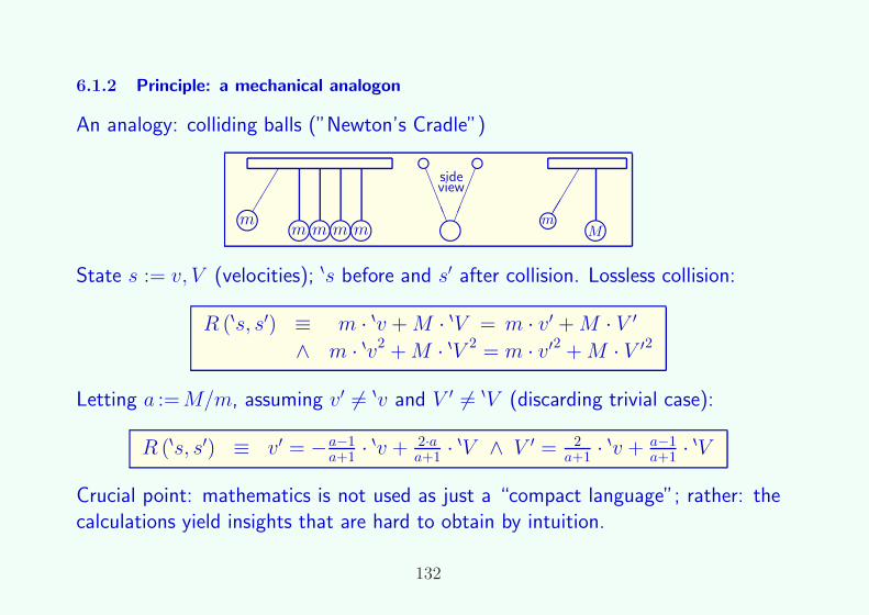
6.1.2 Principle: a mechanical analogon

An analogy: colliding balls (”Newton’s Cradle”)

mm

��

�

mm mm mm mm

f f

m

LLLL

��

��

sideview

jm mM

��

��

State s := v, V (velocities); 8s before and s′ after collision. Lossless collision:

R (8s, s′) ≡ m · 8v + M · 8V = m · v′ + M · V ′∧ m · 8v2 + M · 8V 2 = m · v′2 + M · V ′2

Letting a :=M/m, assuming v′ 6= 8v and V ′ 6= 8V (discarding trivial case):

R (8s, s′) ≡ v′ = −a−1a+1· 8v + 2·a

a+1· 8V ∧ V ′ = 2

a+1· 8v + a−1

a+1· 8V

Crucial point: mathematics is not used as just a “compact language”; rather: thecalculations yield insights that are hard to obtain by intuition.

132

6.2 Calculating the “axioms” for assignment from equations

6.2.0 Principle

a. Basic ideas

• If pre- and postcondition look like propositions, treat them as such

• Derive axiomatic semantics from basic program equations. Convention:

for program variable v, new vars: 8v before command, v′ after command.– Antecondition a becomes a[v8v and postcondition p becomes p[vv′– Substitution and change of variables are familiar in engineering math

– Consider axiomatic semantics just as “economy in variable use”

• Advantages of the approach:– Expressivity: direct formalization of intuitive program behaviour

– Calculationally: all becomes predicate calculus (no “special” logics)

b. Convention

• Mnemonic symbols, even for bound variables (as in physics, applied math)

• We prefer “ante” over “pre” (better preposition, leads to distinct letters)

133

c. Expressing Floyd-Hoare semantics in terms of a program equation

• Side issue: assume v to be of type V (as specified by the declarations)

• Intuitive understanding of behaviour of assignment: equation v′ = e[v8v• Use in formalizing intuitive understanding of Floyd-Hoare semantics:

– About 8v and v′ we know a[v8v and v′ = e[v8v (no less, no more).

– Hence any assertion about v′ must be implied by it, in particular p[vv′.

Formally: a[v8v ∧ v′ = e[v8v⇒ p[vv′ (implicitly quantified over 8v and v′).

{a} v := e {p} ≡ ∀ 8v :V . ∀ v′ : V . a[v8v ∧ v′ = e[v8v⇒ p[vv′ (64)

No detour via denotational semantics; assertions remain propositions.

• Example: assume x declared as integer. Then, by the preceding definition,

{x > 27} x := x+3 {x > 30}≡

∀ 8x : Z . ∀ x′ : Z . 8x > 27 ∧ x′ = 8x + 3⇒ x′ > 30

The latter expression evaluates to 1 (or t if one prefers) by calculation.

134

6.2.1 Calculating the weakest antecondition

• Calculation (assuming type correctness checked, viz., ∀ 8v : V . e[v8v∈ V )

{a} v := e {p} ≡ 〈Definit. (64)〉 ∀ 8v :V . ∀ v′ :V . a[v8v ∧ v′ = e[v8v⇒ p[vv′≡ 〈Shunting〉 ∀ 8v :V . ∀ v′ :V . a[v8v⇒ v′ = e[v8v⇒ p[vv′≡ 〈Ldist ⇒/∀〉 ∀ 8v :V . a[v8v⇒ ∀ v′ :V . v′ = e[v8v⇒ p[vv′≡ 〈One-pt. rule〉 ∀ 8v :V . a[v8v⇒ e[v8v∈ V ⇒ p[ve[v

8v

≡ 〈Assumption〉 ∀ 8v :V . a[v8v⇒ p[ve[v8v

≡ 〈Change vars.〉 ∀ v :V . a⇒ p[ve

• This proves the Theorem: {a} v := e {p} ≡ ∀ v : V . a⇒ p[ve . Hence

– p[ve is at most as strong as any antecondition a.

– p[ve is itself an antecondition since {p[ve} v := e {p} ≡ ∀ v : V . p[ve⇒ p[ve

• Therefore we define wa [[v := e]] p ≡ p[ve (65)

135

6.2.2 Calculating the strongest postcondition

• Calculation

{a} v := e {p} ≡ 〈Definit. (64)〉 ∀ 8v :V . ∀ v′ :V . a[v8v ∧ v′ = e[v8v⇒ p[vv′≡ 〈Swap ∀/∀〉 ∀ v′ :V . ∀ 8v :V . a[v8v ∧ v′ = e[v8v⇒ p[vv′≡ 〈Rdist ⇒/∀〉 ∀ v′ :V . ∃ (8v : V . a[v8v ∧ v′ = e[v8v)⇒ p[vv′≡ 〈Change var〉 ∀ v :V . ∃ (8v : V . a[v8v ∧ v = e[v8v)⇒ p

• Hence Theorem: {a} v := e {p} ≡ ∀ v : V . ∃ (u :V . a[vu∧ v = evu)⇒ p , so

– ∃ (u :V . a[vu∧ v = evu) is at least as strong as any postcondition p.

– ∃ (u :V . a[vu∧ v = evu) is itself a postcondition.

• Therefore we define sp [[v := e]] a ≡ ∃ (u :V . a[vu∧ v = evu) (66)

136

6.2.3 A few interesting excursions / illustrations

a. Justifying the “forward” rule {v = d} v := e {v = e[vd} provided v 6∈ ϕ d

{v = d} v := e {v = e[vd}≡ 〈Definit. (64)〉 ∀ 8v :V . ∀ v′ :V . 8v = d[v8v ∧ v′ = e[v8v⇒ v′ = e[vd[v

v′

≡ 〈v 6∈ ϕ d〉 ∀ 8v :V . ∀ v′ :V . 8v = d ∧ v′ = e[v8v⇒ v′ = e[vd≡ 〈Leibniz, bis〉 ∀ 8v :V . ∀ v′ :V . 8v = d ∧ v′ = e[v8v⇒ e[v8v= e[v8v≡ 〈Reflex. =〉 1 (or t if one prefers)

b. Bouncing ante- and postconditions Letting c := [[v := e]], calculation yields

sp c (wa c p) ≡ p ∧ ∃u :V . v = e[vu wa c (sp c a) ≡ ∃u :V . a[vu∧ e = evu

E.g., assume the declaration y : integer and let c := ‘y := y2 + 7’;furthermore, let p := ‘y > 11’ and q := ‘y < 7’ and a := ‘y > 2’

• sp c (wa c p) ≡ y > 11 ∧ ∃x : Z . y = x2 + 7 (stronger than p !)

• sp c (wa c q) ≡ y < 7 ∧ ∃x : Z . y = x2 + 7 (simplifies to 0 or f)

• wa c (sp c a) ≡ ∃x : Z . x > 2 ∧ y2 + 7 = x2 + 7 (yields y > 2 ∨ y < −2)

137

Recall: sp c (wa c p) ≡ p ∧ ∃u :V . v = e[vu (a)

wa c (sp c a) ≡ ∃u : V . a[vu∧ e = evu (b)

(67)

sp c (wa c q) ≡ 〈Bounce (67a)〉 q ∧ ∃ 8v : V . v = e[v8v≡ 〈Def. q, V , e〉 y < 7 ∧ ∃x : Z . y = x2 + 7≡ 〈Dist. ∧/∃〉 ∃x : Z . y < 7 ∧ y = x2 + 7≡ 〈Leibniz〉 ∃x : Z . x2 + 7 < 7 ∧ y = x2 + 7≡ 〈Arithmetic〉 ∃x : Z . x2 < 0 ∧ y = x2 + 7≡ 〈∀x : Z . x2 ≥ 0〉 ∃x : Z . 0 ∧ y = x2 + 7≡ 〈0 ∧ p ≡ 0〉 ∃x : Z . 0≡ 〈∃ (S • 0) ≡ 0〉 0 (strongest of all propositions)

wa c (sp c a) ≡ 〈Bounce (67b)〉 ∃ 8v :V . a[v8v ∧ e = ev8v

≡ 〈Def. a, V , e〉 ∃x : Z . x > 2 ∧ y2 + 7 = x2 + 7≡ 〈Arithmetic〉 ∃x : Z . x > 2 ∧ (x = y ∨ x = −y)≡ 〈Distr. ∧/∨〉 ∃x : Z . (x = y ∧ x > 2) ∨ (x = −y ∧ x > 2)≡ 〈Distr. ∃/∨〉 ∃ (x : Z . x = y ∧ x > 2) ∨ ∃ (x : Z . x = −y ∧ x > 2)≡ 〈One-pt. rule〉 (y ∈ Z ∧ y > 2) ∨ (−y ∈ Z ∧−y > 2)≡ 〈Arithmetic〉 (y ∈ Z ∧ y > 2) ∨ (y ∈ Z ∧ y < −2)≡ 〈Distr. ∃/∨〉 y ∈ Z ∧ (y > 2 ∨ y < −2) (compare with a)

138

6.3 Generalization to program semantics

6.3.0 Conventions

a. Preliminary remark A familiar “problem”: Given a variable x, we havex ∈ Variable (at metalevel) and, for instance, x ∈ Z (in the language).

Not resolvable without considerable nomenclature, yet clear from the context.Conclusion: let us exploit it rather than lose time over it (at this stage).

Remark: similar (more urgent) problem in calculus: how to “save Leibniz” byformalizing if y = x2, then d y = 2 · x · d x (partial solution 11 years ago)

b. State space

• Not the denotational semantics view where state s : Variable→Value

• State space S is Cartesian product determined by variable declarations.Henceforth, s is shorthand for the tuple of all program variables.

Auxiliary variables (“ghost” or “rigid” variables) appended if necessary.

• Example: var x : int, b : bool yields S = Z×B and s = x, b.

• In what follows, v is a tuple of variables, type Sv, in particular S = Ss.

139

6.3.1 Expressing Floyd-Hoare semantics in terms of program equations

a. Program equations formalizing the intuitive behaviour of command c

• R c (8s, s′) expressing the state change (suitable R :C→S2→B)

• T c s expressing termination of c started in state s (suitable T :C→S→B)In further treatment: only guaranteed, not just possible terminationE.g., not as in the example in Gordon’s Specification and Verification 1,

which would amount (with our conventions) to T c s ≡ ∃ s′ :S . R c (s, s′).

b. Formalizing intuitive Floyd-Hoare semantics for weak correctness

• About 8s and s′ we know a[s8s and R c (8s, s′), no less, no more.

• Therefore: a[s8s ∧Rc (8s, s′) ⇒ p[ss′ (implicitly quantified over 8s and s′).

• Hence {a} c {p} ≡ ∀ 8s :S . ∀ s′ :S . a[s8s ∧R c (8s, s′) ⇒ p[ss′ (68)

c. Strong correctness: defining Term by Term c a ≡ ∀ s :S . a⇒ T c s (69)

[a] c [p] ≡ {a} c {p} ∧ Term c a or, blending in (68):[a] c [p] ≡ ∀ 8s :S . ∀ s′ :S . a[s8s⇒ T c 8s ∧ (Rc (8s, s′) ⇒ p[ss′) (70)

140

6.3.2 Calculating the weakest antecondition

• Calculation

[a] c [p]

≡ 〈Definit. (70)〉 ∀ 8s :S . ∀ s′ :S . a[s8s⇒ T c 8s ∧ (Rc (8s, s′) ⇒ p[ss′)≡ 〈Ldist ⇒/∀〉 ∀ 8s :S . a[s8s⇒ ∀ s′ :S . T c 8s ∧ (Rc (8s, s′) ⇒ p[ss′)≡ 〈Pdist ∀/∧〉 ∀ 8s :S . a[s8s⇒ T c 8s ∧ ∀ s′ :S . R c (8s, s′) ⇒ p[ss′≡ 〈Change vars.〉 ∀ s :S . a⇒ T c s ∧ ∀ s′ :S . R c (s, s′) ⇒ p[ss′

• So we proved [a] c [p] ≡ ∀ s :S . a⇒ T c s ∧ ∀ s′ :S . R c (s, s′) ⇒ p[ss′

– Observe, as before, that T c s ∧ ∀ s′ :S . R c (s, s′) ⇒ p[ss′ is

at most as strong as any antecondition a and is itself an antecondition

– Hence wa c p ≡ T c s ∧ ∀ s′ :S . R c (s, s′) ⇒ p[ss′ (71)

• Liberal variant: wla c p ≡ ∀ s′ :S . R c (s, s′) ⇒ p[ss′ (72)

(shortcut: obtained by substituting T c s ≡ 1)

141

6.3.3 Calculating the strongest postcondition

• Calculation

[a] c [p]

≡ 〈Def. (68–70)〉 Term c a ∧ ∀ 8s :S . ∀ s′ :S . a[s8s ∧Rc (8s, s′) ⇒ p[ss′≡ 〈Swap ∀〉 Term c a ∧ ∀ s′ :S . ∀ 8s :S . a[s8s ∧Rc (8s, s′) ⇒ p[ss′≡ 〈Rdist ⇒/∀〉 Term c a ∧ ∀ s′ :S . ∃ (8s :S . a[s8s ∧R c (8s, s′))⇒ p[ss′≡ 〈Change var〉 Term c a ∧ ∀ s :S . ∃ (8s :S . a[s8s ∧R c (8s, s))⇒ p

• So we proved [a] c [p] ≡ Term c a ∧ ∀ s :S . ∃ (8s :S . a[s8s ∧R c (8s, s))⇒ p

– Assuming Term c a, observe, as before, that ∃ 8s :S . a[s8s ∧R c (8s, s) is at

least as strong as any postcondition p and is itself a postcondition

– Hence sp c p ≡ ∃ 8s :S . a[s8s ∧R c (8s, s) provided Term c a (73)

• Liberal variant: slp c p ≡ ∃ 8s :S . a[s8s ∧R c (8s, s) (74)

142

6.4 Application to assignment, sequencing, choice and iteration

6.4.0 Assignment revisited (embedded in the general case)

a. We consider (possibly) multiple assignment Let c := [[v := e]]

• Here v may be a tuple of variables and e a matching tuple of expressions.

• Convenient in calculations: (W.L.O.G.) s = v ++ w (w rest of variables);similarly 8s = 8v ++ 8w and s′ = v′++ w′

b. Formalizing intuitive understanding (note simplest choice of bound variables)

R c (s, s′) ≡ s′ = s[ve (75)

T c s ≡ 1

E.g., R [[y,j := y+j,j+1]] ((y, j, k), (y′, j′, k′)) ≡ y′, j′, k′ = y + j, j + 1, k

c. Weakest ante- and strongest postconditions From (71) and (73) with (75),

wa [[v := e]] p ≡ p[ve (76)sp [[v := e]] a ≡ ∃ 8v : Sv . a[v8v ∧ v = e[v8v (77)

143

6.4.1 Sequencing

a. Formalization of intuitive understanding of behaviour

R [[c′; c′′]] (8s, s′) ≡ ∃ t :S . R c′ (8s, t) ∧R c′′ (t, s′)T [[c′; c′′]] s ≡ T c′ s ∧ ∀ t :S . R c′ (s, t)⇒ T c′′ t (78)

b. Weakest antecondition (strongest postcondition similar) Let c := [[c′; c′′]] in

wa c p

≡ 〈Eqn. wa (71)〉 T c s ∧ ∀ s′ :S . R c (s, s′) ⇒ p[ss′≡ 〈Def. R (78)〉 T c s ∧ ∀ s′ :S . ∃ (t :S . R c′ (s, t) ∧R c′′ (t, s′)) ⇒ p[ss′≡ 〈Rdist. ⇒/∀〉 T c s ∧ ∀ s′ :S . ∀ t :S . R c′ (s, t) ∧ R c′′ (t, s′) ⇒ p[ss′≡ 〈Rearrange〉 T c s ∧ ∀ t :S . R c′ (s, t)⇒ ∀ s′ :S . R c′′ (t, s′) ⇒ p[ss′≡ 〈Blend T (78)〉 T c′ s ∧ ∀ t :S . R c′ (s, t)⇒ T c′′ t ∧ ∀ s′ :S . R c′′ (t, s′) ⇒ p[ss′≡ 〈Eqn. wa (71)〉 T c′ s ∧ ∀ t :S . R c′ (s, t)⇒ (wa c′′ p)[st≡ 〈Eqn. wa (71)〉 wa c′ (wa c′′ p)

Remark: Gordon observes that this could not be obtained by T c s ≡ ∃ t :S . R c (s, t)

144

6.4.2 Choice (nondeterministic; deterministic as particular case)

a. Formalizing intuitive understanding Let ch := [[if i : I . bi -> ci fi]] in

R ch (s, s′) ≡ ∃ i : I . bi ∧ R ci (s, s′) (79)

T ch s ≡ ∀ i : I . bi ⇒ T ci s

Remark: I is just a (finite) indexing set, say, 0 ..n− 1 for n alternatives.

b. Weakest ante-, strongest postcondition Let ch := [[if i : I . bi -> ci fi]] in

wa ch p ≡ 〈Eqn. wa (71)〉 T ch s ∧ ∀ s′ :S . R ch (s, s′)⇒ p[ss′≡ 〈Def. R (79)〉 T ch s ∧ ∀ s′ :S . ∃ (i : I . bi ∧R ci (s, s

′))⇒ p[ss′≡ 〈Rdist ⇒/∃〉 T ch s ∧ ∀ s′ :S . ∀ i : I . bi ∧ R ci (s, s

′)⇒ p[ss′≡ 〈Shunt, dist.〉 T ch s ∧ ∀ i : I . bi ⇒ ∀ s′ :S . R ci (s, s

′)⇒ p[ss′≡ 〈Blend T (79)〉 ∀ i : I . bi ⇒ T ci s ∧ ∀ s′ :S . R ci (s, s

′)⇒ p[ss′≡ 〈Eqn. wa (71)〉 ∀ i : I . bi ⇒ wa ci p

sp ch a ≡ 〈Similar calc.〉 ∃ i : I . sp ci (a ∧ bi), provided Term c a

c. Particular case: defining [[if b then c′ else c′′ fi]] = [[if b -> c′ ¬ b -> c′′ fi]]

yields wa [[if b then c′ else c′′ fi]] p ≡ (b⇒ wa c′ p) ∧ (¬ b⇒ wa c′′ p)

145

6.4.3 Iteration

a. Formalizing intuitive understanding Let l := [[do b -> c od]] in what follows.

Then l = [[if ¬ b -> skip b -> c ; l fi]] formalizes intuition about behaviour.

b. Calculating R l, T l and wa l Using the earlier results, (head) calculation yields:

R l (s, s′) ≡ (¬ b⇒ s = s′) ∧ (b⇒ ∃ t :S . R c (s, t) ∧R l (t, s′)) (80)T l s ≡ (¬ b⇒ 1) ∧ (b⇒ T c s ∧ ∀ t :S . R c (s, t)⇒ T l t) (81)

wa l p ≡ (¬ b⇒ p) ∧ (b⇒ wa c (wa l p)) (82)

Equivalently: wa l p ≡ (¬ b ∧ p) ∨ (b∧ wa c (wa l p)). Unfolding suggests defining

wn+1 l p ≡ (¬ b ∧ p) ∨ (b ∧ wa c (wn l p))w0 l p ≡ ¬ b ∧ p

By induction, one can prove ∀n : N . wn l p⇒ wa l p so ∃ (n : N . wn l p)⇒ wa l p

c. Bounded nondeterminism: extra requirement T l s ⇒ ∃ (n : N . dn l s) whered0 l s ≡ ¬ b and dn+1 l s ≡ b ⇒ T c s ∧ ∀ t :S . R c (s, t) ⇒ dn l t (# steps ≤ n).

Then wa l p ≡ ∃ (n : N . wn l p) (as in Dijkstra’s A Discipline of Programming).

146

6.5 Practical rules for iteration

Let D be a set with order < and W :P D a well-founded subset under <. Thenan expression e of type D is a bound expression for c iff (i) ∀ s • b ⇒ e ∈ W ; (ii)

∀w :W . [b ∧ w = e] c′ [e < w]. Combining:

Definition: i : B and e : D are an invariant/bound pair for c iff

(i) ∀ s • i ∧ b⇒ e ∈ W and (ii) ∀w :W . [i ∧ b ∧ w = e] c′ [i ∧ e < w]

We can prove the following theorem.

Theorem: If i, e is an invariant/bound pair for c then [i] c [i ∧ ¬ b] (83)

Using (83) in practice is best done via a checklist, as suggested by Gries: to show[a] do b -> c′ od [p], find suitable i, e and prove

(i) i satisfies [i ∧ b] c′ [i] or, equivalently, i ∧ b⇒ wa c′ i.(ii) i satisfies a⇒ i.(iii) i satisfies i ∧ ¬ b⇒ p.

(iv) e satisfies i ∧ b⇒ e ∈ W .(v) e satisfies i ∧ b ∧ w = e⇒ wa c′ (e < w) for any w : W .

147

Next topic








Lecture C: Applications in computer and software engineering16:05–16:40 5. Applications of generic functionals in computing science




148

7 Formal calculation as unification with classical engineering

7.0 Applications in analysis: calculation replacing syncopation

7.1 Applications in continuous and general systems theory

7.2 Applications in discrete systems theory

7.3 Closing remarks: a discipline of Electrical and Computer Engineering

149

7.0 Analysis: calculation replacing syncopation — an example

def ad : (R→B)→ (R→B) with ad P v ≡ ∀ ǫ : R>0 . ∃x : RP . |x− v| < ǫdef open : (R→B)→B with

open P ≡ ∀ v : RP . ∃ ǫ : R>0 . ∀x :R . |x− v| < ǫ⇒ P xdef closed : (R→B)→B with closedP ≡ open (¬P )

Example: proving the closure property closedP ≡ ad P = P .

closedP≡ 〈Definit. closed〉 open (¬P )

≡ 〈Definit. open〉 ∀ v : R¬P . ∃ ǫ : R>0 . ∀x : R . |x− v| < ǫ⇒ ¬P x≡ 〈Trading sub ∀〉 ∀ v : R .¬P v ⇒ ∃ ǫ : R>0 . ∀x : R . |x− v| < ǫ⇒ ¬P x

≡ 〈Contrapositive〉 ∀ v : R .¬∃ (ǫ : R>0 . ∀x : R . P x⇒ ¬ (|x− v| < ǫ))⇒ P v≡ 〈Duality, twice〉 ∀ v : R . ∀ (ǫ : R>0 . ∃x : R . P x ∧ |x− v| < ǫ)⇒ P v

≡ 〈Definition ad〉 ∀ v : R . adP v ⇒ P v≡ 〈P v ⇒ ad P v〉 ∀ v : R . adP v ≡ P v (proving P v ⇒ ad P v is near-trivial)

150

7.1 Applications in continuous and general systems theory

7.1.0 Transform methods

a. Emphasis: formally correct use of functionals; clear and unambiguous bindings

Avoiding common defective notations like F {f(t)} and writing F f ω instead

F f ω =

∫ +∞

−∞e−j·ω·t · f t · d t F ′g t = 1

2 · π ·∫ +∞

−∞ej·ω·t · g ω · d ω

b. Example: formalizing Laplace transforms via Fourier transforms.

Auxiliary function: ℓ—

: R→R→R with ℓσ t = (t < 0) ? 0 e−σ·t

We define the Laplace-transform L f of a function f by:

L f (σ + j · ω) = F (ℓσ · f) ω

for real σ and ω, with σ such that ℓσ · f has a Fourier transform.

With s := σ + j · ω we obtain

L f s =

∫ +∞

0

f t · e−s·t · d t .

151

c. Calculation example: the inverse Laplace transform

Specification of L′: L′ (L f) t = f t for all t ≥ 0

(weakened where ℓσ · f is discontinous).

Calculation of an explicit expression: For t as specified,

L′ (L f) t = 〈Specification〉 f t

= 〈eσ·t · ℓσ t = 1〉 eσ·t · ℓσ t · f t

= 〈Definition 〉 eσ·t · (ℓσ · f) t

= 〈Weakened〉 eσ·t · F ′ (F (ℓσ · f)) t

= 〈Definition F ′〉 eσ·t · 12·π ·

∫ +∞−∞ F (ℓσ · f) ω · ej·ω·t · d ω

= 〈Definition L〉 eσ·t · 12·π ·

∫ +∞−∞ L f (σ + j · ω) · ej·ω·t · d ω

= 〈Const. factor〉 12·π ·

∫ +∞−∞ L f (σ + j · ω) · e(σ+j·ω)·t · d ω

= 〈s := σ + j·ω〉 12·π·j ·

∫ σ+j·∞σ−j·∞ L f s · es·t · d s

152

7.1.1 Characterization of properties of systems

a. Definitions and conventions

Define SA = T→A for value space A and time domain T. Then

• A signal is a function of type SA

• A system is a function of type SA→SB.

Note: the response of s :SA→SB to input signal x :SA at time t : T is s x t.Recall: s x t is read (s x) t, not to be confused with s (x t).

153

b. Characteristics Let s :SA→SB. Then:

• System s is

memoryless iff ∃ f— : T→A→B . ∀x :SA . ∀ t : T . s x t = ft (x t)

• Let T be additive, and the shift function σ— be defined by

στ x t = x (t + τ) for any t and τ in T and any signal x. Then s is

time-invariant iff ∀ τ : T . s ◦στ = στ ◦ s

• Let now s :SR→SR. Then system s is linear iff

∀ (x, y) :S2R

. ∀ (a, b) :R2 . s (a⇀· x + b

⇀· y) = a⇀· s x + b

⇀· s y.

Equivalently, extending s to SC→SC in the evident way, system s is

linear iff ∀ z :SC . ∀ c : C . s (c⇀· z) = c

⇀· s z

• A system is LTI iff it is both linear and time-invariant.

154

c. Response of LTI systems

Define the parametrized exponential E— : C→T→C with Ec t = ec·t

Then we have:

Theorem: if s is LTI then s Ec = s Ec 0⇀· Ec

Proof: we calculate s Ec (t + τ) to exploit all properties.

s Ec (t + τ) = 〈Definition σ〉 στ (s Ec) t

= 〈Time inv. s〉 s (στ Ec) t

= 〈Property Ec〉 s (Ec τ⇀· Ec) t

= 〈Linearity s〉 (Ec τ⇀· s Ec) t

= 〈Defintion⇀〉 Ec τ · s Ec t

Substituting t := 0 yields s Ec τ = s Ec 0 · Ec τ or, using⇀

,s Ec τ = (s Ec 0

⇀· Ec) τ , so s Ec = sEc 0⇀· Ec by function equality.

The 〈Property Ec〉 is στ Ec = Ec τ⇀· Ec (easy to prove).

Note that this proof uses only the essential hypotheses.

155

7.2 Applications in discrete systems theory

7.2.0 Motivation and chosen topic

Automata: classical common ground between computing and systems theory.Even here formalization yields unification and new insights.

Topic: sequentiality and the derivation of properties by predicate calculus.

7.2.1 Sequential discrete systems

a. Discrete systems: signals of type A∗ (or B∗), and systems of type A∗→B∗.

b. Sequentiality Define ≤ on A∗ (or B∗ etc.) by x ≤ y ≡ ∃ z :A∗ . y = x ++ z.

System s is non-anticipatory or sequential iff x ≤ y ⇒ s x ≤ s y

Function r : (A∗)2→B∗ is a residual behavior of s iff s (x ++ y) = s x ++ r (x, y)

Now we can prove:

Theorem: s is sequential iff it has a residual behavior function.

(proof: next)

156

Proof: we start from the sequentiality side.

∀ (x, y) : (A∗)2 . x ≤ y ⇒ s x ≤ s y≡ 〈Definit. ≤〉 ∀ (x, y) : (A∗)2 . ∃ (z : A∗ . y = x ++ z)⇒ ∃ (u :B∗ . s y = s x ++ u)

≡ 〈Rdst ⇒/∃〉 ∀ (x, y) : (A∗)2 . ∀ (z : A∗ . y = x ++ z ⇒ ∃u : B∗ . s y = s x ++ u)≡ 〈Nest, swp〉 ∀x :A∗ . ∀ z :A∗ . ∀ (y : A∗ . y = x ++ z ⇒ ∃u :B∗ . s y = s x ++ u)

≡ 〈1-pt, nest〉 ∀ (x, z) : (A∗)2 . ∃u :B∗ . s (x ++ z) = s x ++ u≡ 〈Compreh.〉 ∃ r : (A∗)2→B∗ . ∀ (x, z) : (A∗)2 . s (x ++ z) = s x ++ r (x, z)

We used the function comprehension axiom: for any relation R : X ×Y →B,

∀ (x :X . ∃ y : Y . R (x, y)) ≡ ∃ f : X→Y . ∀x :X . R (x, f x)

157

7.2.2 Derivatives and primitives

The preceding framework leads to the following.

a. Observation: An rb function is unique (exercise).

b. We define the derivation operator D on sequential systems by

D s ε = ε and D s (x−< a) = s x ++D s (x−< a)

With the rb function r of s, D s (x−< a) = r (x, τ a).

c. Primitivation I is defined for any g :A∗→B∗ by

I g ε = ε and I g (x−< a) = I g x ++ g (x ++ a)

158

d. Properties (a striking analogy from analysis is shown in the second row)

s (x−< a) = s x ++ D s (x−< a) s x = s ε ++ I (D s) xf (x + h) ≈ f x + D f x · h f x = f 0 + I (D f) x

In the second row, D is derivation as in analysis, and I g x =∫ x

0 g y · d y.

e. The state space is {(y :A∗ . r (x, y)) | x :A∗}.If we replace r by its Curried version, the state space is {r x | x :A∗}

159

7.3 Closing remarks: a discipline of ECE

a. What we have shown

• A formalism with a very simple language and powerful formal rules

• Notational and methodological unification

of CS and other engineering theories

• Unification also encompassing a large part of mathematics.

b. Ramifications

• Scientific: obvious (deepens insight, consolidates knowledge, reduces frag-

mentation, expands intuition, suggests solutions, exploits analogies etc.)

• Educational: unified basis for ECE (Electrical and Computer Engineering)

Possible curriculum structure:

– Formal calculation at early stage

– Other engineering math courses rely on it and provide consolidation

160

Tutorial — ICTAC 2004 Functional Predicate Calculus and ... · Functional Predicate Calculus and...

Documents

Transcript of Tutorial — ICTAC 2004 Functional Predicate Calculus and ... · Functional Predicate Calculus and...