1

Tutorial 5

River and Lake Boundary Conditions

Table of Contents

Objective …………………………………………………………………………………. 1

Step-by-Step Procedure ……………………………………………………………….... 2

Section 1 – Specification of Lake Boundary Conditions ………………………………… 2

Step 1: Open Adaptive Groundwater Input (.agw) File …………………………………. 2

Step 2: Add Lake Boundary Condition ………………………………………………….. 3

Step 3: Add Lake Boundary Condition (cont.) ………………………………………….. 3

Step 4: Add Lake Boundary Condition (cont.) ………………………………………….. 4

Step 5: Define Lake Hydraulic Properties ……………………………………………….. 6

Step 6: Save Lake Data …………………………………………………………………... 7

Section 2 – Specification of River Boundary Conditions ………………………………… 7

Step 1: Assign River Boundary Condition ………………………………………………. 7

Step 2: Assign River Boundary Condition (cont.) ………………………………………. 7

Step 3: Assign River Boundary Condition (cont.) ………………………………………. 9

Step 4: Enter River Hydraulic Properties ……………………………………………….. 9

Step 5: Save River Data ………………………………………………………………… 10

Step 6: Review Input Data and Boundary Conditions …………………………………... 11

Section 3 – Simulation Results Visualization …………………………………………….. 13

Step 1: View Plan View Hydraulic Head Contour Map …………………………………. 13

Step 2: View Plan View Hydraulic Head Contour Map (cont.) …………………………. 14

Step 3: Contour Map Overlays …………………………………………………………… 15

Step 4: Plot Velocity Vectors, Zoom In/Out, and Translate ……………………………… 16

Step 5: View x-z Cross-Section Contour (Line) Plot of Hydraulic Heads ………………. 17

Objective

Illustrate the incorporation of river and lake (leaky-type) boundary conditions. The completed

Adaptive Groundwater input files for this tutorial are included in the Tutorial_5 subdirectory of

the tutorials directory under the Adaptive_Groundwater program folder:

C:\Adaptive_Groundwater\Tutorials\Tutorial_5\Tutorial_5_Completed.agw

2

Because Tutorial 5 builds upon the input data and boundary conditions for Tutorial 1, you can

refer to this first tutorial for illustrations of basic input data preparation (e.g., grid design, basic

boundary condition specification, time step control, etc.). The completed Tutorial 5 project files

are provided to you as a reference (you can check the completed input data if you have questions

while working through the tutorial). Many output times are also provided so that you can view

the variations of hydraulic heads and solute concentrations over a long time period. As discussed

below, you will work with a separate set of project files.

This tutorial is divided into three sections. The first part covers boundary condition

specifications for lakes (Section 1) and rivers (Section 2). Section 3 shows how to create various

visualizations of the simulation results for this tutorial.

Step-by-Step Procedure

Section 1 – Specification of Lake Boundary Conditions

Step 1 - Open Adaptive Groundwater Input (.agw) File

Go to File > Open in the main menu to open the file Tutorial_5_Start.agw that is stored in the

following subdirectory:

C:\Adaptive_Groundwater\Tutorials\Tutorial_5

The Base Grid is initially displayed on the screen (Figure 1).

3

Figure 1

Step 2 – Add Lake Boundary Condition

Start by adding a lake boundary condition in the top layer of the model Base Grid (Figure 1). In

the main menu select Boundary Conditions > River or Lake > Lake > Assign. The Assign Lake

Boundary Conditions dialog box pops up (Figures 2 and 3). If you want to review a full

discussion of the parameter values for this dialog select the “Help” button.

Step 3 – Add Lake Boundary Condition (cont.)

Change the “Current Layer” to 10 (Figure 2), which is the top layer of the Base Grid.

Note: Lake and river B.C.’s are assigned vertically based on the lake or river “Bed Elevation”

(i.e., the top of the sediment layer). Boundary conditions are assigned on a layer-by-layer basis

and to any elevation within a layer. As discussed in the “Help” section, the final B.C.

4

assignment to cells is performed during the simulation once the degree of mesh refinement has

been finalized for a given time step.

Figure 2

Step 4 – Add Lake Boundary Condition (cont.)

Use your left mouse button to sketch out a lake boundary in plan view that looks similar to the

one in Figure 3. (Enter hydraulic parameter values for the lake after drawing the geometry.) Use

the “Esc” key at any time to abort the drawing of the lake boundary polygon.

When finished, push the right mouse button to complete the lake boundary. The “Define

Boundary Condition Characteristics” dialog appears to remind you to enter your site-specific

lake parameter values (Figure 3). Click on the “OK” button and the entered lake boundary is

drawn (Figure 4).

Note: As part of the input data display, the boundaries of Base Grid cells that are intersected by

the lake are also highlighted in color when the lake geometry is drawn. However, during a

simulation lake B.C.’s are assigned based on the finer cell sizes on higher levels of AMR

refinement (refer to “Help”).

5

Figure 3

6

Figure 4

Step 5 – Define Lake Hydraulic Properties

Now, enter the lake parameter values listed in the completed dialog box shown in Figure 2.

Define the lake bed elevation (top of the lake bed layer), where “bed elevation limits” shows the

allowable range based on the current Base Grid layer selection (i.e., upper and lower surface of

the current layer). Enter the lake bed thickness, blake (the lake bed extends vertically from the

lake bed elevation to a distance blake below the bed surface).

The lake bed permeability (Klake) can be entered as either the actual value (m/day) or as the ratio

of the lake bed permeability to the vertical aquifer hydraulic conductivity, (Kz)aquifer [ Klake /

(Kz)aquifer ≤ 1.0 ]. For example, Klake / (Kz)aquifer = 0.001 sets the lake bed permeability to a

factor of 1,000 lower than (Kz)aquifer for any cell on any level of AMR refinement. As an

illustration, assuming a correlated random hydraulic conductivity field is used to define the

7

aquifer then the lake bed permeability would also be random and equal to a factor of 1,000 lower

than (Kz)aquifer at every cell that contains the lake bed.

“Lake Head” is the fixed hydraulic head at the top of the lake bed (e.g., lake water surface

elevation).

For “Lake Concentration” enter any negative value if you want the “Default Inflow

Concentrations” value to be used for defining the concentration of any lake flux (i.e., any cell

located within the lake bed boundary) that is outward (i.e., flow is from the lake into the aquifer).

If “lake concentration” is nonzero, the specified value will be used to define the outward lake

flux concentration.

Step 6 – Save Lake Data

Make to sure to “Save” your selections for this lake boundary condition before exiting this B.C.

option. “Cancel” to abort the lake definition without saving your input.

Section 2 – Specification of River Boundary Conditions

Defining a river is analogous to the lake entry described above. However, river parameter values

may linearly vary from one river centerline coordinate to another.

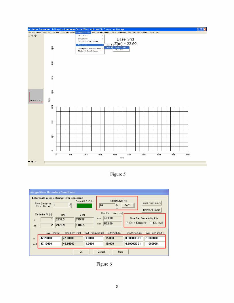
Step 1 – Assign River Boundary Condition

Start by adding a river in the top layer of the model Base Grid. In the main menu select

Boundary Conditions > River or Lake > River > Assign (Figure 5). The Assign River Boundary

Conditions dialog box pops up (Figure 6). If you want to review a full discussion of the

parameter values for this dialog select the “Help” button.

Step 2 – Assign River Boundary Condition (cont.)

Change the “Current Layer” to 10 (Figure 6), which is the top layer of the Base Grid.

8

Figure 5

Figure 6

9

Step 3 – Assign River Boundary Condition (cont.)

Use your left mouse button to sketch out a river centerline in plan view that looks similar to the

one in Figure 7 (3 centerline points; 2 river segments). (Enter hydraulic parameter values for the

river after drawing the geometry.) Use the “Esc” key at any time to abort the drawing of the

river centerline.

When finished, push the right mouse button to complete the river centerline. The “Define River

Characteristics” dialog appears to remind you to enter your site-specific river parameter values.

Click on the “OK” button and the entered river geometry is drawn (Figure 7).

Note: As part of the input data display, the boundaries of Base Grid cells that are intersected by

the river are also highlighted in color when the river geometry is drawn. However, during a

simulation river B.C.’s are assigned based on the finer cell sizes on higher levels of AMR

refinement (refer to “Help”).

Step 4 – Enter River Hydraulic Properties

Now, enter the river parameter values listed in the completed dialog box shown in Figure 6.

Define the river bed elevation (top of the river bed layer), where “bed elevation limits” shows the

allowable range based on the current Base Grid layer selection (i.e., upper and lower surface of

the current layer). This example uses river bed elevations of 47.0, 46.9, and 46.8 m for the three

centerline coordinates. All river parameters are linearly interpolated between centerline points.

Enter the river bed thickness, briver (the river bed extends vertically from the bed elevation to a

distance briver below the bed surface). A uniform bed thickness of 1.0 m is used in this example.

“Bed Width” is the plan-view width of the river bed (measured normal to the centerline). This

example uses bed widths of 15, 10, and 5 m at the three centerline coordinates.

The river bed permeability (Klake) can be entered as either the actual value (m/day) or as the ratio

of the river bed permeability to the vertical aquifer hydraulic conductivity, (Kz)aquifer [ Kriver /

(Kz)aquifer ≤ 1.0 ]. For example, Kriver / (Kz)aquifer = 0.001 sets the river bed permeability to a

factor of 1,000 lower than (Kz)aquifer for any cell on any level of AMR refinement. As an

illustration, assuming a correlated random hydraulic conductivity field is used to define the

aquifer then the river bed permeability would also be random and equal to a factor of 1,000

lower than (Kz)aquifer at every cell that contains the lake bed. Kriver / (Kz)aquifer = 0.03 is used in

this example.

“River Head” is the fixed hydraulic head at the top of the river bed (e.g., river water surface

elevation). This example uses river heads of 47.2, 47.1, and 47.0 m for centerline coordinates 1-

3.

10

For “River Concentration” enter any negative value if you want the “Default Inflow

Concentrations” value to be used for defining the concentration of any river flux (i.e., any cell

located within the river bed boundary) that is outward (i.e., flow is from the river into the

aquifer). If “river concentration” is nonzero, the specified value will be used to define the

outward river flux concentration. This example uses a uniform river concentration of -1.

Step 5 – Save River Data

Make to sure to “Save” your selections for this river boundary condition before exiting this B.C.

option. “Cancel” to abort the river definition without saving your input.

Figure 7

11

Step 6 – Review Input Data and Boundary Conditions

You can review the model input data and boundary conditions at any time by selecting Review

Input on the main menu, which pops up the dialog box in Figure 8. Push “Show Selection” to

inspect an input data type or boundary condition from the drop-down menu (left click on a B.C.

or material zone to view the input values). Use the checkboxes to add desired B.C. overlays to

each plot.

In this example, we show Hydraulic Conductivity (one uniform K zone) with overlays of the

Hydraulic Head and Lake/River boundary conditions for this tutorial (Figure 9). Figure 10 is a

corresponding x-z cross-section view with vertical exaggeration.

Figure 8

12

Figure 9

13

Figure 10

Section 3 – Simulation Results Visualization

In this section we show how to create various two-dimensional plots of the simulation results for

Tutorial 5. You can use either the supplied Tutorial_5_Completed project files or your working

copy of the Adaptive Groundwater files for this tutorial: Tutorial_5_Start.agw. It does not

matter if you have made new runs with shorter simulation times than those shown here; select

whatever output time that you want.

Step 1 – View Plan View Hydraulic Head Contour Map

In the main menu select Output > Hydraulic Head and the View Simulation Results dialog

appears (Figure 11). A plan-view flood map through the middle of the aquifer is automatically

generated. Click the “Go To” button at the top of the dialog to pop up a child dialog with

14

available output times; click on any output time you want and select “OK” in the “Go to Output

Time” dialog. You may also use the “+” / “-“ buttons to toggle through the output times.

Under Plot and Contour Types you see that “2D” (i.e., two-dimensional) plots are the default.

Change the “Contour Type” to lines.

Figure 11

Step 2 – View Plan View Hydraulic Head Contour Map (cont.)

Use the slice plane “Go To” button (Figure 11) to change the view-plane elevation to 47.03 m

and the plot in Figure 12 is generated.

You can also click the Layer no. “+/-“ buttons (Figure 11). Further, you can view an animation

of the different plan-view slices by changing the “Animation Type” to Layer (K-plane) and

clicking the “Start Animation” button.

Note: the layer number refers to the Adaptive Mesh Refinement (AMR) mesh associated with

the multi-level AMR grid created during the simulation. In highly-refined mesh areas the

vertical discretization is equal to the grid spacing in the highest-level subgrid (e.g, Level 5 in this

example which utilizes five AMR levels). In less-refined areas the grid layer thickness for the

output is equal to the grid spacing in the most-refined subgrid (e.g., Level 1, 2, 3, or 4).

A total of 40 head contour intervals are used in the range 47.5 to 52.5 m. To change the contour

intervals select “Contour Options” in the View Simulation Results dialog and click the

15

“Contouring Options” tab in the Contour Parameters and Overlays child dialog (Figure 13). If

you wish to use any of these display options later, click on the “Save Plot Format” button at the

bottom of the View Simulation Results dialog (Figure 11).

Step 3 – Contour Map Overlays

Figure 12 also consists of these overlays: the AMR mesh, pathlines, and river/lake boundary

conditions. The mesh overlay can be turned off by un-checking the “Mesh” box in the Contour

Options dialog (under the “Overlays” tab; Figure 13).

If groundwater pathline starting locations are defined in the input data (Pathlines > Assign in the

main menu) their computed trajectories can be shown in the output by checking the “Show

Pathlines” box in the Contour Options dialog (under the Pathlines tab; Figure 13). Display

overlays of the lake and river boundary conditions by checking “River & Lake B.C.’s” under the

“Overlays” tab.

Figure 12

16

Figure 13

Step 4 – Plot Velocity Vectors, Zoom In/Out, and Translate

Figure 14 is a close-up view of the hydraulic head distribution near the river and lake, and pore

velocity vectors (activate under the “Vectors” tab in the Contour Options dialog). You can

change the vector length [“V Length(%)”] and spacing (“Vector Indices Skip”) by selecting the

Vectors tab in the Contour Options dialog.

In all plots you can “Zoom In”, “Zoom Last”, or “Translate” the view by clicking one of the

icons in the upper-left corner of the display (Figure 12) or by making the appropriate selection

under View in the main menu.

17

Figure 14

Step 5 – View x-z Cross-Section Contour (Line) Plot of Hydraulic Heads

To display the cross-sectional view in Figure 15, click on the X-Z Slice (Row) button in the

lower left hand corner (red circle), and then select a row of cells (i.e., x-z slice) that cuts through

both the river and lake (or select View > Change View Plane in the main menu). When you first

switch to the cross-section view, you will want to add vertical exaggeration (e.g., VE = 10-20) by

going to View > Vertical Exaggeration in the main menu.

Figure 16 is a close-up view of the hydraulic head contours and the pore velocity vectors beneath

the river and lake.

18

Figure 15

19

Figure 16