Turing Machines andDifferential Linear Logic

James Clift

Supervisor: Daniel Murfet

Masters Thesis

The University of Melbourne

Department of Mathematics and Statistics

October 2017

Abstract

We describe the vector space semantics for linear logic in which the exponential modalityis modelled by cofree coalgebras. There is a natural differentiable structure in thissemantics arising from the primitive elements. We provide an investigation of thisstructure, through many examples of proofs and their derivatives. In particular, anencoding of Turing machines in linear logic is given in detail, based on work by Girard,but modified in order to be compatible with derivatives. It is shown that for proofs ofthe appropriate form, the derivatives obtained via the coalgebraic structure agree withthose from elementary calculus, allowing one to write Taylor expansions of proofs. Weprovide an interpretation of the derivative of the Turing encoding via a simple example.

Contents

1 Introduction 1

2 Linear logic 42.1 Preliminaries . . . . . . . . . . . . . . . . . . . . . . . . . . . . . . . . 42.2 The Sweedler semantics . . . . . . . . . . . . . . . . . . . . . . . . . . 9

3 Denotations and derivatives 133.1 Booleans . . . . . . . . . . . . . . . . . . . . . . . . . . . . . . . . . . . 133.2 Integers . . . . . . . . . . . . . . . . . . . . . . . . . . . . . . . . . . . 143.3 Binary integers . . . . . . . . . . . . . . . . . . . . . . . . . . . . . . . 203.4 Iteration and copying . . . . . . . . . . . . . . . . . . . . . . . . . . . . 26

4 Syntax of differential linear logic 29

5 Turing machines 335.1 The encoding . . . . . . . . . . . . . . . . . . . . . . . . . . . . . . . . 355.2 Copying . . . . . . . . . . . . . . . . . . . . . . . . . . . . . . . . . . . 445.3 Nondeterministic Turing machines . . . . . . . . . . . . . . . . . . . . . 46

6 Polynomiality and Taylor series 48

A Polynomiality of Turing machines 55

Acknowledgements : Many thanks to my wonderful supervisor Daniel Murfet formany hours of engaging conversation and invaluable advice. Thanks to my friends forhelping me endure the stress which comes along with higher education. Lastly, thankyou to my family, particularly my parents, for fostering my love of mathematics from avery young age.

1 Introduction

In the 1930s the notion of computability was given a rigorous definition in twodifferent but equivalent forms. These are:

1. The λ-calculus, developed by Church, wherein computation is carried out byreducing terms in the language to a normal form.

2. Turing machines, developed by Turing, wherein computation is imagined as afinite state machine with unbounded memory following a simple set of rules.

In the terminology of computer science, the former is the prototypical example of func-tional programming, and the latter of imperative programming.

Given that the same class of functions N → N may be encoded by both λ-calculusand Turing machines, one could reasonably describe the question of computability assettled. In this thesis, we will consider the broader question of the structure of the set ofall computer programs. Our model of computation is that of linear logic – introducedby Girard in the 1980s – into which simply typed λ-calculus embeds [8]. The logicrestricts the use of the weakening and contraction rules of traditional intuitionisticlogic to certain classes of formulas, so that the only formulas which may be duplicatedor discarded are those preceded by a new operator ‘!’, called the exponential. This givesa natural interpretation of the logic as being resource conscious: if a premise withoutthe exponential appears in a logical argument, one can be sure that this premise is usedprecisely once; that is, in a linear way. The logic has the advantage of being able tocompute almost any total function of integers one could possibly hope for, while stillbeing strongly normalising ; no computation can run forever.

A convenient lens through which one can study linear logic is its semantics : a wayof mapping the syntax of proofs into familiar categorical structures [12, §2]. This issimilar to the way in which representation theory provides an understanding of groupsvia linear maps of vector spaces. Originally, a semantics of linear logic in coherencespaces was provided by Girard [8], and since then a wide variety of other semanticshave been proposed [3, 4]. Our particular focus will be a vector space semantics (theSweedler semantics), which assigns to each logical formula A a vector space JAK, andto each proof π of Γ ` A a linear map JπK : JΓK → JAK. In the Sweedler semantics,the exponential !A is assigned the cofree coalgebra generated by JAK, and the means toencode nonlinear maps is provided by the grouplike elements of the coalgebra [13].

Somewhat more interestingly, the cofree coalgebra comes with an intrinsic differen-tiable structure via the primitive elements. Precisely, a proof π of !A ` B has, for eachγ ∈ JAK, an associated linear map

∂γJπK : JAK→ JBK,

which is analogous to the derivative of a smooth map of manifolds at the point γ. Itis important to emphasise that the differentiable structure is not artificially added to

1

the semantics; it naturally appears as soon as one considers cofree coalgebras. Giventhat proofs in linear logic correspond to computer programs which one would typicallythink of as being discrete objects, the appearance of differentiation – which seems torequire continuity – comes as a surprise. We therefore consider it prudent to investigatethis structure fully. The appearance of derivatives in linear logic is not new; the roleof differentiable structure on the λ-calculus and linear logic has been motivated by itsconnection to head normal forms [20, 17]. However, in our view there is still a lack ofelementary examples of proofs whose derivatives have clear computational meaning.

In this thesis we will attempt to fill this gap by providing such examples. Manyfamiliar data types, including booleans and binary integers, can easily be encoded inlinear logic. By this, we mean that there exists a formula bintA in linear logic suchthat any binary sequence can be encoded as a proof of ` bintA. For a more involvedexample, we will show that there is an encoding of Turing machines into linear logic.One can encode the instantaneous configuration of Turing machine as a proof of

TurA = !bintA ⊗ !bintA ⊗ !nboolA,

and the state evolution of a Turing machine is described by a proof δstepA

of

TurA3 ` TurA.

The idea of encoding Turing machines in linear logic is by no means a new development;originally this arose in connection with polynomial time complexity [25], and a variety ofencodings exist in the literature [24, 19]. Our work is specifically based on an encodingdue to Girard [9], but is novel in the sense that it does not require the use of second orderquantifiers. Our justification for this change is twofold. Firstly, the Sweedler semanticshas no obvious extension to second order linear logic, and so one cannot understandthe logic algebraically; in particular, any link to differentiation is lost. Secondly, theuse of second order quantification undermines the resource sensitivity that linear logicattempts to capture; in second order linear logic, there are ways to copy binary integersarbitrarily many times via a proof of bint ` !bint.

In Section 2 we define the syntax and terminology of linear logic, review the basictheory of coalgebras, and define the Sweedler semantics of linear logic. A wealth ofexamples of data types and functions which may be encoded in linear logic are givenin Section 3. We provide a proof that the Sweedler semantics is injective on integersand binary integers. In Section 4, we explain how one can interpret the differentiablestructure in the syntax by adjoining new deduction rules. In Section 5, we present ourencoding of Turing machines in linear logic. An encoding of nondeterministic Turingmachines is also provided. Connections to derivatives in the sense of elementary calculusare discussed in Section 6. We show that proofs of an appropriate form have denotationswhich can be expanded as a Taylor series. In particular this applies to δstep

A, and we

give an interpretation of the derivative in terms of the operation of the machine.

2

axiomA ` A

Γ, A,B,∆ ` Cexch

Γ, B,A,∆ ` CΓ ` A ∆, A ` B

cutΓ,∆ ` B

Γ, A ` C&L0

Γ, A&B ` CΓ, B ` C

&L1Γ, A&B ` C

Γ ` A Γ ` B&R

Γ ` A&B

Γ, A,B ` C⊗L

Γ, A⊗B ` CΓ ` A ∆ ` B ⊗R

Γ,∆ ` A⊗B

Γ ` A ∆, B ` C( L

Γ,∆, A( B ` CΓ, A ` B

( RΓ ` A( B

Γ, A ` Bder

Γ, !A ` B!Γ ` A prom!Γ ` !A

Γ ` Bweak

Γ, !A ` BΓ, !A, !A ` B

ctrΓ, !A ` B

Figure 1.1: Sequent calculus for linear logic. The symbols A,B,C are formulas, andthe symbols Γ,∆ are sequences of formulas, possibly empty. The notation !Γ in thepromotion rule ‘prom’ means that each formula in Γ is preceded by an exponentialmodality.

3

2 Linear logic

2.1 Preliminaries

We begin by introducing the terminology of first-order intuitionistic linear logic,hereafter referred to as linear logic. Fix a collection of atomic variables {x1, x2, ...}. Thenotion of a formula (or type) is defined recursively as follows: each atomic variableis a formula, and if A and B are formulas then so are (A&B), (A ⊗ B), (A ( B)and !A. The operator ‘!’ is called the exponential modality. A sequent is a non-empty sequence of formulas (A1, ..., An, B) where n ≥ 0, written as A1, ..., An ` B. Theformulas A1, ..., An are called the premises and the formula B is called the conclusion,the idea being that the formula B can be deduced from the formulas A1, ..., An. Thesymbol ` is called the turnstile. A sequent may have any number of premises, evennone, but must have precisely one conclusion. Sequences of formulas are usually denotedby upper case Greek letters.

The sequent calculus (Figure 1.1) for linear logic allows us to deduce the validityof some sequents from others. Proofs are inductively built by starting from axioms(tautological sequents of the form A ` A) and applying deduction rules. More precisely,a proof is a rooted plane tree whose vertices are labelled by sequents, such that allleaves are axioms and such that each node and its children correspond to one of thededuction rules in Figure 1.1. Typically when writing a proof we omit exchange rulesto improve readability, treating the left hand side of a sequent as an unordered list.

Example 2.1. Consider the following proof:

A ` AB ` B C ` C

( LA,A( B ` B

( LA,A( B,B ( C ` C

( RA( B,B ( C ` A( C

If one thinks of a proof of ` A( B as being a function A→ B, the above proof may beinterpreted as composition of the two inputs to obtain a single output of type A( C.

Of particular significance is the ‘cut’ rule, which encapsulates modus ponens for thelinear implication, (. Perhaps surprisingly, this rule turns out to be unnecessary fromthe point of view of provability.

Theorem 2.2. (Hauptsatz.) If π is a proof of Γ ` A, then there exists a proof π′ ofΓ ` A in which there is no occurrence of the cut rule.

Moreover, there is an effective procedure to transform π into π′, outlined in [8, 12].It is this cut elimination procedure which gives rise to the computational interpretationof linear logic; the cut rule should be understood as being composition of proofs, andperforming cut elimination is analogous to performing β-reduction in the λ-calculus. Itis the process that transforms π to π′ which is important, not merely the existence of

4

π′. We write π →cut π′ to mean that π reduces to π′ under cut elimination, and define

∼cut as the smallest equivalence relation containing →cut.Let C be a symmetric monoidal category [16]. A categorical semantics [12] for

linear logic assigns to each formula A an object of C denoted JAK, and to each proof πof A1, ..., An ` B a morphism JπK : JA1K⊗ ...⊗ JAnK→ JBK, such that if π ∼cut π

′ thenJπK = Jπ′K. The objects and morphisms are called denotations.

Our aim is to define a vector space semantics for linear logic. As is typical, the bulkof the work is to obtain a suitable interpretation of the exponential !A. To do this, wefirst review the basic theory of coalgebras from [2]. Let k be a field.

Definition 2.3. A coassociative counital coalgebra over k is a k-vector space Cequipped with linear maps ∆ : C → C ⊗ C and ε : C → k, called the coproduct andcounit respectively, such that the following diagrams commute:

C C ⊗ C

C ⊗ C C ⊗ C ⊗ C

∆

∆ id⊗∆

∆⊗id

C

C ⊗ k C ⊗ C k ⊗ C

∆∼=∼=

ε⊗idid⊗ε

The coalgebra C is cocommutative if the following diagram also commutes, whereσ : C ⊗ C → C ⊗ C is the map σ(a⊗ b) = b⊗ a:

C C ⊗ C

C ⊗ C

∆

∆σ

Given two coalgebras (C1,∆1, ε1) and (C2,∆2, ε2) over k, a coalgebra morphism fromC1 to C2 is a k-linear map Φ : C1 → C2 such that the following diagrams commute:

C1 C1 ⊗ C1

C2 C2 ⊗ C2

∆1

Φ Φ⊗Φ

∆2

C1 C2

k

ε1

Φ

ε2

From here on, all coalgebras are coassociative, counital and cocommutative.

Example 2.4. If A is a finite-dimensional (unital) algebra with multiplication map∇ : A ⊗ A → A and unit η : k → A, then its dual A∗ can be equipped with thestructure of a coalgebra. The coproduct ∆ is the composite

A∗∇∗−−−−−−→ (A⊗ A)∗

∼=−−−−−−→ A∗ ⊗ A∗.

The isomorphism (A⊗A)∗ ∼= A∗ ⊗A∗ is natural in A, but an explicit description of ∆requires a choice of basis. If {v1, ..., vn} is a basis of A with dual basis {v1, ..., vn}, then

5

the value of ∆(ϕ) for ϕ ∈ A∗ is given by

ϕ 7−−−−−−→ ϕ ◦ ∇ 7−−−−−−→n∑

i,j=1

ϕ(vivj)(vi ⊗ vj).

The counit of A∗ is simply η∗ followed by the canonical isomorphism k∗ ∼= k.

Definition 2.5. Let C be a coalgebra. An element x ∈ C is called grouplike [22]if ∆(x) = x ⊗ x and ε(x) = 1. We denote the set of grouplike elements by G(C). Ifx ∈ G(C), an element y ∈ C is called primitive over x if ∆(y) = x⊗ y + y ⊗ x. Theset of primitive elements over x is denoted Px(C), and we write P (C) for the union ofall such Px(C).

Lemma 2.6. Coalgebra morphisms send grouplike elements to grouplike elements, andprimitive elements to primitive elements.

Proof. Let (C,∆C , εC) and (D,∆D, εD) be coalgebras and Φ : C → D a coalgebramorphism. If x ∈ G(C) then ∆DΦ(x) = (Φ ⊗ Φ)∆C(x) = Φ(x) ⊗ Φ(x) and εDΦ(x) =εC(x) = 1, so Φ(x) ∈ G(D). Likewise, if y ∈ Px(C) then ∆DΦ(y) = (Φ ⊗ Φ)∆C(y) =Φ(x)⊗ Φ(y) + Φ(y)⊗ Φ(x), so Φ(y) ∈ PΦ(x)(D).

Given a morphism of coalgebras Φ : C → D, there is therefore an induced functionon grouplike elements G(Φ) : G(C)→ G(D), and so we have a functor

G : Coalg→ Set.

Similarly, for x ∈ G(C) there is an induced map on primitive elements Px(Φ) : Px(C)→PΦ(x)(D) which is also functorial.

Lemma 2.7. Let C be a coalgebra. There exist natural bijections:

• HomCoalg(k, C)→ G(C) given by Φ 7→ Φ(1), and

• HomCoalg((k[t]/t2)∗, C)→ P (C) given by Φ 7→ Φ(t∗).

Proof. If Φ : k → C is a morphism of coalgebras, then Φ(1) is grouplike in C by theprevious lemma. Conversely, any grouplike element x ∈ C induces a unique morphismof coalgebras Φ : k → C given by Φ(a) = ax, and hence G(C) ∼= HomCoalg(k, C).

Let T = (k[t]/t2)∗, which has the dual basis {1∗, t∗}. From the discussion in Example2.4, the coproduct ∆ on T is given by

∆(1∗) = 1∗ ⊗ 1∗, ∆(t∗) = 1∗ ⊗ t∗ + t∗ ⊗ 1∗,

and the counit ε byε(1∗) = 1, ε(t∗) = 0.

Hence t∗ is primitive over 1∗. If Φ : T → C is a morphism of coalgebras, it follows thatΦ(t∗) is primitive over Φ(1∗). Since any primitive element y ∈ C over x ∈ G(C) givesrise to a morphism of coalgebras Φ : T → C via Φ(1∗) = x, Φ(t∗) = y, we concludethat P (C) ∼= HomCoalg(T,C).

6

Let V be the category of vector spaces over k and C the category of (coassociative,counital, cocommutative) coalgebras over k. As proven in [2, Theorem 4.1], the forgetfulfunctor U : C → V has a right adjoint F : V → C .

Definition 2.8. Let V be a vector space. The coalgebra F (V ) is called the cofreecoalgebra generated by V , and we write !V for the underlying vector space UF (V ).The counit of adjunction d : !V → V is called the dereliction map. We will oftenwrite !V to instead mean the coalgebra F (V ) itself; the meaning will always be clearfrom context.

The coalgebra !V is unique up to unique isomorphism. The universal property ofthe dereliction map tells us that for any coalgebra C and any linear map ϕ : C → V ,there is a unique lifting of ϕ to a morphism of coalgebras Φ = promϕ : C → !V calledthe promotion of ϕ, such that d ◦ Φ = ϕ. Indeed, the adjunction between F and Uimplies that the map Homk(C, V )→ HomCoalg(C, !V ) which sends ϕ to its promotionis a bijection.

In order to understand the structure of !V , our first step is to determine the grouplikeand primitive elements. By Lemma 2.7 and the universal property of !V , we have anatural bijection

G(!V ) ∼= HomCoalg(k, !V ) ∼= Homk(k, V ) ∼= V.

The grouplike element of !V corresponding to v ∈ V is denoted |∅〉v and is called thevacuum vector at v. Explicitly, the linear map ϕ : k → V associated to v ∈ V isϕ(a) = av, the lifting is Φ(a) = a|∅〉v, and hence

d(|∅〉v) = d(Φ(1)) = ϕ(1) = v.

Similarly, for the primitive elements we have

P (!V ) ∼= HomCoalg(T, !V ) ∼= Homk(T, V ) ∼= V × V,

where T = (k[t]/t2)∗. We denote the primitive element associated to (v, w) ∈ V × Vby |w〉v ∈ !V . The associated linear map ϕ : T → V is given by 1∗ 7→ v, t∗ 7→ w, andthe lifting Φ : T → !V is 1∗ 7→ |∅〉v, t∗ 7→ |w〉v, and thus we have

d(|w〉v) = d(Φ(t∗)) = ϕ(t∗) = w.

Remark 2.9. The role of the dual numbers k[t]/t2 gives a geometric interpretation of|w〉v as the tangent vector at v in the direction of w. This can be made precise viaalgebraic geometry; see [13, Appendix B]. Briefly, if X is a scheme and p ∈ X is a closedpoint, the tangent space of X at p is TpX = (m/m2)∗, where m ⊆ OX,p is the maximalideal. It is well known [10, §VI.1.3] that specifying a closed point p ∈ X and a tangentvector w ∈ TpX is equivalent to specifying a morphism of k-schemes Spec(k[t]/t2)→ X.In particular, if X = Spec(Sym(V ∗)) then scheme morphisms Ψ : Spec(k[t]/t2) → X

7

correspond to elements of P (!V ) (that is, pairs of vectors in V ) via the following naturalbijections [15]:

HomSch/k(Spec(k[t]/t2), Spec(Sym(V ∗)) ∼= HomAlg(Sym(V ∗), k[t]/t2)∼= Homk(V

∗, k[t]/t2)∼= Homk ((k[t]/t2)∗, V )∼= P (!V ).

We now give an explicit description of !V in the case where V is finite-dimensional,following [13, 14]. Assume that k is algebraically closed and of characteristic zero. Byresults of Sweedler [22, Chapter 8], any cocommutative coalgebra over an algebraicallyclosed field can be written as a direct sum of its irreducible components, and eachirreducible component contains a unique grouplike element. By the above, the irre-ducible components are therefore in bijection with elements of V . Given that k hascharacteristic zero, if (!V )γ denotes the irreducible component of !V containing |∅〉γ, wehave (!V )γ ∼= Sym(V ) as coalgebras for each γ ∈ V , where Sym(V ) is the symmetriccoalgebra [14, Lemma 2.18]. We therefore have

!V =⊕γ∈V

(!V )γ ∼=⊕γ∈V

Sym(V ).

Generalising the notation already used for the grouplike and primitive elements:

Definition 2.10. The equivalence class of α1⊗...⊗αn in the copy of Sym(V ) associatedto γ ∈ V is denoted by a ket |α1, ..., αn〉γ. The empty tensor at γ is denoted |∅〉γ.

With this notation, the coproduct and counit are given by

∆|α1, ..., αn〉γ =∑I⊆[n]

|αI〉γ ⊗ |αIc〉γ and ε|α1, ..., αn〉γ =

{1 n = 0

0 n > 0

where [n] = {1, ..., n} and for a (possibly empty) subset I = {i1, ..., ik} ⊆ [n] we write|αI〉γ to mean |αi1 , ..., αik〉γ. The dereliction map d : !V → V is given by

d|α1, ..., αn〉γ =

γ n = 0

α1 n = 1

0 n > 1.

If ϕ : !V → W is a linear map then the promotion [14, Theorem 2.22] Φ : !V → !W canbe written explicitly as

Φ|α1, ..., αn〉γ =∑

P∈P([n])

∣∣∣ϕ|αP1〉γ, ..., ϕ|αPm〉γ⟩ϕ|∅〉γ

where P([n]) denotes the set of partitions of [n].

8

The explicit description above assumes that V is finite-dimensional. In the casewhere V is infinite-dimensional, one can write V as the direct limit of its finite-dimensional subspaces Vi, in which case !V = lim−→ !Vi. In this case, any element of!V can still be written as a finite sum of kets, and so the formulas for the coproduct,counit, dereliction map and promotion remain the same [14, Section 2.1].

2.2 The Sweedler semantics

Definition 2.11. We recursively define the denotation JAK of a formula A. For eachatomic formula xi, we choose a finite-dimensional k-vector space JxiK. For formulasA,B, define:

• JA&BK = JAK⊕ JBK,

• JA⊗BK = JAK⊗ JBK,

• JA( BK = Homk(JAK, JBK),

• J!AK = !JAK.

If Γ is A1, ..., An, then we define JΓK = JA1K⊗ ...⊗ JAnK.

Definition 2.12. Let π be a proof of Γ ` B. The denotation JπK is a linear mapJπK : JΓK → JBK which is defined recursively on the structure of proofs. The proof πmust match one of the proofs in the first column of the following table, and the secondtable defines its denotation. Here, d denotes the dereliction map, ∆ the coproduct, andpromϕ the promotion of ϕ as in Definition 2.8.

axiomA ` A JπK(a) = a

π1...Γ, A,B,∆ ` C

exchΓ, B,A,∆ ` C

JπK(γ ⊗ b⊗ a⊗ δ) = Jπ1K(γ ⊗ a⊗ b⊗ δ)

π1...Γ ` A

π2...∆, A ` B

cutΓ,∆ ` B

JπK(γ ⊗ δ) = Jπ2K(δ ⊗ Jπ1K(γ))

π1...Γ, A ` C

&L0Γ, A&B ` C

JπK(γ ⊗ (a, b)) = Jπ1K(γ ⊗ a)

9

π1...Γ, B ` C

&L1Γ, A&B ` C

JπK(γ ⊗ (a, b)) = Jπ1K(γ ⊗ b)

π1...Γ ` A

π2...Γ ` B

&RΓ ` A&B

JπK(γ) = (Jπ1K(γ), Jπ2K(γ))

π1...Γ, A,B ` C

⊗LΓ, A⊗B ` C

JπK(γ ⊗ (a⊗ b)) = Jπ1K(γ ⊗ a⊗ b)

π1...Γ ` A

π2...∆ ` B ⊗R

Γ,∆ ` A⊗BJπK(γ ⊗ δ) = Jπ1K(γ)⊗ Jπ2K(δ)

π1...Γ ` A

π2...∆, B ` C

( LΓ,∆, A( B ` C

JπK(γ ⊗ δ ⊗ ϕ) = Jπ2K(δ ⊗ ϕ ◦ Jπ1K(γ))

π1...Γ, A ` B

( RΓ ` A( B

JπK(γ) = {a 7→ Jπ1K(γ ⊗ a)}

π1...Γ, A ` B

derΓ, !A ` B

JπK(γ ⊗ a) = Jπ1K(γ ⊗ d(a))

π1...!Γ ` A prom!Γ ` !A

JπK = promJπ1K

π1...Γ ` B

weakΓ, !A ` B

JπK(γ ⊗ a) = Jπ1K(γ)

π1...Γ, !A, !A ` B

ctrΓ, !A ` B

JπK(γ ⊗ a) = Jπ1K(γ ⊗∆(a))

Table 2.1: Denotations of proofs in the Sweedler semantics.

10

Since the exponential is modelled through the cofree coalgebra, we have the abilityto encode nonlinear maps as follows:

Definition 2.13. Let π be a proof of !A ` B. There is an associated nonlinear mapJπKnl : JAK→ JBK defined by JπKnl(γ) = JπK|∅〉γ.

Example 2.14. The fact that the function γ 7→ γ ⊗ γ is nonlinear is captured by thefact that there is no proof of A ` A⊗ A for a generic formula A in linear logic. Thereis however always a proof π of !A ` A⊗ A:

A ` A A ` A ⊗RA,A ` A⊗ A

der!A,A ` A⊗ A

der!A, !A ` A⊗ A

ctr!A ` A⊗ A

The denotation of π is JπK = (d⊗ d) ◦∆, and so the associated nonlinear map is

JπKnl(γ) = (d⊗ d) ◦∆|∅〉γ = d|∅〉γ ⊗ d|∅〉γ = γ ⊗ γ.

In this sense, JπKnl validates our intuition that the proof π is ‘copying’ the input.

We can give an alternative description of JπKnl. Let π′ be the promotion of π to aproof of !A ` !B. Then JπKnl can be defined as the composite:

JAK∼=−−−−−−→ G(!JAK)

G(Jπ′K)−−−−−−→ G(!JBK)

∼=−−−−−−→ JBKγ 7−−−−−−→ |∅〉γ 7−−−−−−→ |∅〉JπK|∅〉γ

7−−−−−−→ JπK|∅〉γ.

The fact that this map is nonlinear is a consequence of the fact that for c, d ∈ k andγ, δ ∈ JAK we generally have:

c|∅〉γ + d|∅〉δ 6= |∅〉cγ+dδ.

There is also a map which corresponds to taking the image of the primitive elementsof !JAK under Jπ′K. If γ ∈ JAK, and writing γ = |∅〉γ, consider the composite:

JAK∼=−−−−−−→ Pγ(!JAK)

Pγ(Jπ′K)−−−−−−→ PJπK(γ)(!JBK)∼=−−−−−−→ JBK.

Denote this composite by ∂γJπK. It is easily verified that ∂γJπK is linear1. This is rem-iniscent of ideas from differential geometry; recall that if M,N are smooth manifolds,p ∈ M and F : M → N is a smooth map, the derivative of F at p (Figure 2.1) isa linear map TpF : TpM → TFpN between the tangent spaces, thought of as the bestlinear approximation to F at p. Given our interpretation of |α〉γ as a tangent vector atγ in the direction of α (Remark 2.9), it is reasonable to understand the map ∂γJπK asbeing analogous Tγ(JπKnl). In summary:

1Note that the dependence on γ is generally nonlinear.

11

M

N

••p

Fpv

TpF (v)F−−−−−−−−→

Figure 2.1: The derivative of a smooth map.

Definition 2.15. Let π be a proof of !A ` B, and γ ∈ JAK. There is an associatedlinear map ∂γJπK : JAK → JBK given by ∂γJπK(α) = JπK|α〉γ, called the coalgebraicderivative of JπK at γ. We also write ∂JπK : JAK × JAK → JBK for the (nonlinear)function given by ∂JπK(α, γ) = JπK|α〉γ.

One of our goals in the next section is to justify this analogy, by showing that inmany cases, the coalgebraic derivative really does behave as one would expect fromelementary calculus.

12

3 Denotations and derivatives

Many simple data types such as booleans, integers and binary integers have a naturalencoding as proofs in linear logic. We now provide a variety of examples of such proofsand their coalgebraic derivatives. In doing so, we hope the reader will develop a senseof the types of programming that is possible within linear logic.

3.1 Booleans

Definition 3.1. Let A be a formula. The type of booleans on A is

boolA = (A&A) ( A.

The two values of a boolean correspond to the following proofs 0A and 1A of ` boolA:

A ` A&L0

A&A ` A( R` boolA

A ` A&L1

A&A ` A( R` boolA

whose denotations are projection onto the zeroth and first coordinates respectively.Note that we are using the convention that the left introduction rules for & are indexedby 0 and 1, rather than by the more conventional choice of 1 and 2, in order to beconsistent with the usual assignment of 0 as ‘false’ and 1 as ‘true’.

A boolean can be used to ‘choose’ between two proofs π0, π1 of Γ ` A, via thefollowing proof ρ:

π0...Γ ` A

π1...Γ ` A

&RΓ ` A&A A ` A

( LΓ,boolA ` A

The denotation of this proof is the map

JρK(γ ⊗ ϕ) = ϕ(Jπ0K(γ), Jπ1K(γ))

for γ ∈ JΓK and ϕ ∈ JboolAK. In particular, if ϕ = JiAK, then this simplifies to

JρK(γ ⊗ JiAK) = JπiK(γ).

The above construction easily generalises to provide an encoding of n-booleans in linearlogic; that is, elements of the set {0, ..., n− 1}. Let An = A& ...&A where there are ncopies of A.

Definition 3.2. Let n ≥ 2. The type of n-booleans on A is nboolA = An ( A.

The n possible values of an n-boolean correspond to the projection maps proji :JAnK → JAK, where i ∈ {0, ..., n − 1}. We denote by iA the proof of ` nboolA whosedenotation is proji; that is:

13

A ` A&Li

An ` A( R` nboolA

Here, by &Li (0 ≤ i ≤ n − 1) we mean the rule which introduces n − 1 new copies ofA on the left, such that the original A is at position i, indexed from left to right.

3.2 Integers

Another familiar data type which may be encoded in linear logic is that of integers.The idea is the same as that which is used in λ-calculus, in which the natural number nis encoded as the term λf.λx.fnx; that is, the function (f, x) 7→ fn(x). Of course, sucha function has a nonlinear dependence on f , which suggests the following definition.

Definition 3.3. The type of integers on A is the formula

intA = !(A( A) ( (A( A).

Definition 3.4. Let comp0A

be the proof A ` A. We recursively define compnA

for n ∈ Nas the proof

A ` A

compn−1

A...A, (n− 1) (A( A) ` A

( LA, n (A( A) ` A

where n (A( A) is notation for n copies of A( A.

An easy computation shows that JcompnAK : JAK ⊗ JA ( AK⊗n → JAK is the map

a⊗ f1 ⊗ ...⊗ fn 7→ (fn ◦ ... ◦ f1)(a); note that the ordering of the fi is reversed.For n ∈ N, there is a proof2 nA of ` intA given by

compnA...

A, nA( A ` An× der

A, n !(A( A) ` A(n− 1)× ctr

A, !(A( A) ` A( R

!(A( A) ` A( A( R` intA

2It will sometimes be convenient to exclude the final ( R rule, instead writing nA as a proofof !(A ( A) ` A ( A. This is reasonable since Homk(U ⊗ V,W ) and Homk(U,Homk(V,W )) arecanonically isomorphic by currying, and semantically the ( R rule corresponds to one direction ofthis isomorphism. We will usually not distinguish between proofs containing rules such as ( L or ⊗L,and the corresponding proofs with those rules removed.

14

called the Church numeral for n. We occasionally drop the subscript A and simplywrite n when doing so will not cause confusion.

In order to describe the denotation of nA, for sets X, Y let Inj(X, Y ) denote the setof all injective functions X → Y .

Proposition 3.5. For n > 0 the denotation of nA is the linear map

JnAK : !JA( AK→ JA( AK

given by

JnAK|α1, ..., αk〉γ =∑

f∈Inj([k],[n])

Γfn ◦ · · · ◦ Γf1 ,

where α1, ..., αk, γ ∈ JA( AK = End(JAK) and

Γfi =

{αf−1(i) i ∈ im(f)

γ i /∈ im(f).

In particular, JnAK vanishes on |α1, ..., αk〉γ if k > n.

Intuitively speaking, the value of JnAK|α1, ..., αk〉γ is the sum over all ways of replac-ing k of the copies of γ in the composite γn with the maps α1, ..., αk.

Proof. It is easily seen that JnAK = JcompnAK ◦ d⊗n ◦ ∆n−1. The image of |α1, ..., αk〉γ

under n− 1 contractions is ∑I1,...,In

|αI1〉γ ⊗ ...⊗ |αIn〉γ

where the sum ranges over all sequences of subsets I1, ..., In ⊆ [k] which are pairwisedisjoint and such that I1 ∪ ... ∪ In = [k]. Applying d⊗n annihilates any term of thesum which contains a ket of length greater than one. Any summand which remainscorresponds to a choice of k distinct elements of [n], or equivalently an injective function[k]→ [n]. Finally, compn

Acomposes the operators.

Corollary 3.6. For α, γ ∈ JA( AK, we have

JnAKnl(γ) = γn and ∂γJnAK(α) =n∑i=1

γi−1αγn−i.

It is in this sense that the Church numeral nA can be thought of as encoding thenonlinear function (f, x) 7→ fn(x). Moreover, at least in this simple example, there isa clear connection between the coalgebraic derivative and the ordinary tangent map ofsmooth manifolds:

15

Example 3.7. With k = C and JAK = Cn, let X = J2AKnl : Mn(C)→Mn(C), which isthe map γ 7→ γ2. For 1 ≤ a, b ≤ n let Xa,b : Mn(C) → C denote the component of Xobtained by projecting onto the ath row and bth column. Explicitly, for γ ∈Mn(C) wehave:

Xa,b(γ) =n∑i=1

γa,iγi,b.

This is a smooth map of real manifolds with tangent map TγX : TγMn(C)→ Tγ2Mn(C).Under the identification TγMn(C) = Tγ2Mn(C) = Mn(C), for matrices α, γ ∈ Mn(C),the matrix TγX(α) ∈Mn(C) has entries:

(TγX)a,b(α) =∑

1≤c,d≤n

αc,d∂Xa,b

∂γc,d

=∑

1≤c,d≤n

αc,d(δa,cγd,b + δb,dγa,c)

=n∑d=1

αa,dγd,b +n∑c=1

αc,bγa,c

= (αγ + γα)a,b,

where δ is the Kronecker delta. So the tangent map TγX agrees with ∂γJ2AK, and by asimilar computation one can show that the same holds for any Church numeral mA.

We will shortly present some examples of the kinds of functions of integers whichcan be encoded in linear logic. To justify their computational meaning, we will typicallyargue semantically rather than by actually performing the cut elimination procedure onthe proofs themselves. A priori, this is not sufficient since the computational meaning ofthe proof is a syntactic notion, and just because two proofs have the same denotationdoes not guarantee that they are equivalent under cut elimination. Fortunately forintegers, this turns out to be the case.

Proposition 3.8. Let A be a formula with dimJAK > 0. The set {JnAK}n≥0 is linearlyindependent in JintAK.

Proof. Suppose that∑n

i=0 ciJiK = 0 for some scalars c0, ..., cn ∈ k. Let p ∈ k[x] be thepolynomial p =

∑ni=0 cix

i. For α ∈ JA( AK we have

p(α) =n∑i=0

ciαi =

n∑i=0

ciJiK|∅〉α = 0.

The minimal polynomial of α therefore divides p. Since this holds for any linear mapα ∈ JA( AK, it follows that p is identically zero, as k is characteristic zero.

Corollary 3.9. The function N→ JintAK given by n 7→ JnAK is injective.

16

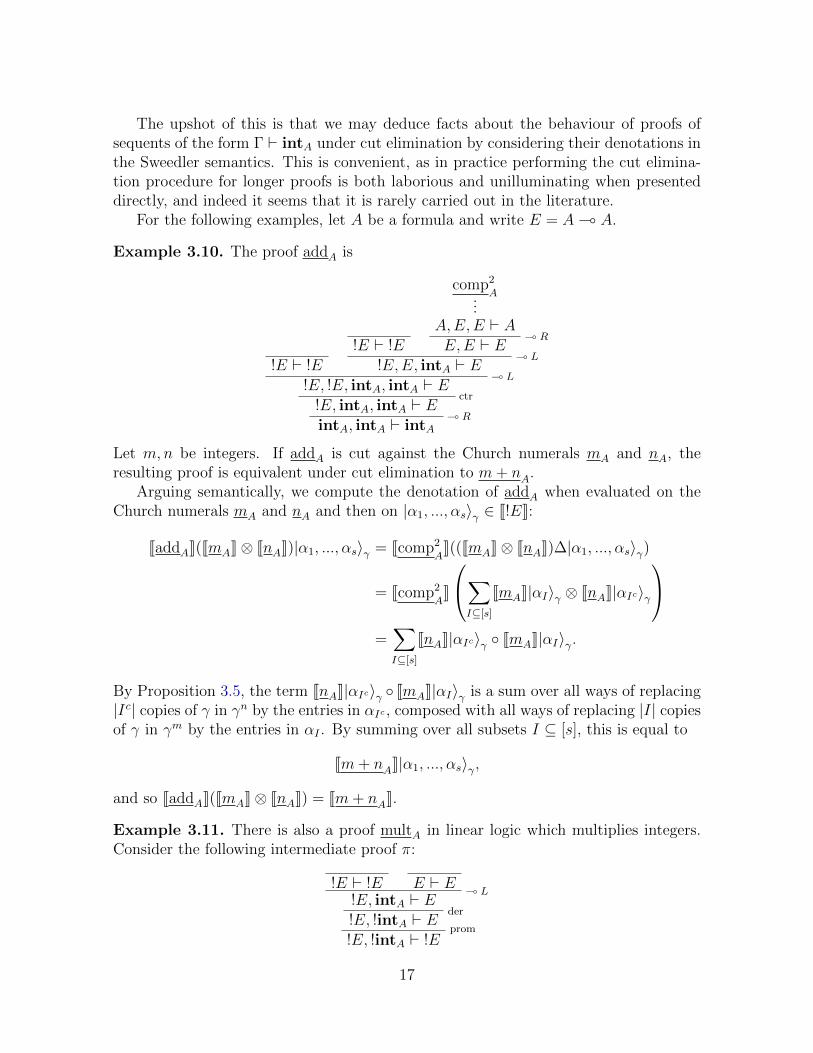
The upshot of this is that we may deduce facts about the behaviour of proofs ofsequents of the form Γ ` intA under cut elimination by considering their denotations inthe Sweedler semantics. This is convenient, as in practice performing the cut elimina-tion procedure for longer proofs is both laborious and unilluminating when presenteddirectly, and indeed it seems that it is rarely carried out in the literature.

For the following examples, let A be a formula and write E = A( A.

Example 3.10. The proof addA is

!E ` !E

!E ` !E

comp2

A...A,E,E ` A

( RE,E ` E

( L!E,E, intA ` E

( L!E, !E, intA, intA ` E

ctr!E, intA, intA ` E

( RintA, intA ` intA

Let m,n be integers. If addA is cut against the Church numerals mA and nA, theresulting proof is equivalent under cut elimination to m+ nA.

Arguing semantically, we compute the denotation of addA when evaluated on theChurch numerals mA and nA and then on |α1, ..., αs〉γ ∈ J!EK:

JaddAK(JmAK⊗ JnAK)|α1, ..., αs〉γ = Jcomp2

AK((JmAK⊗ JnAK)∆|α1, ..., αs〉γ)

= Jcomp2

AK

∑I⊆[s]

JmAK|αI〉γ ⊗ JnAK|αIc〉γ

=∑I⊆[s]

JnAK|αIc〉γ ◦ JmAK|αI〉γ.

By Proposition 3.5, the term JnAK|αIc〉γ ◦ JmAK|αI〉γ is a sum over all ways of replacing|Ic| copies of γ in γn by the entries in αIc , composed with all ways of replacing |I| copiesof γ in γm by the entries in αI . By summing over all subsets I ⊆ [s], this is equal to

Jm+ nAK|α1, ..., αs〉γ,

and so JaddAK(JmAK⊗ JnAK) = Jm+ nAK.

Example 3.11. There is also a proof multA in linear logic which multiplies integers.Consider the following intermediate proof π:

!E ` !E E ` E( L

!E, intA ` Eder

!E, !intA ` E prom!E, !intA ` !E

17

Then JπK : ! EndJAK⊗ !JintAK→ ! EndJAK is a morphism of coalgebras such that

JπK(x⊗ |∅〉γ) = |∅〉γ(x) and JπK(x⊗ |α〉γ) = |α(x)〉γ(x),

for any α, γ ∈ JintAK = Homk(! EndJAK,EndJAK). Using π, we can write down theproof multA which corresponds to multiplying two integers:

π...!E, !intA ` !E E ` E

( L!E, !intA, intA ` E

( R!intA, intA ` intA

Now let l,m, n be integers and write γ = JlK and α = JmK. Then the coalgebraicderivative of multA(−, n) at α in the direction of γ is (for t ∈ J!EK):

JmultAK(|α〉γ ⊗ JnK)(t) = JnK(|α(t)〉γ(t)) =n∑i=1

γ(t)i−1α(t)γ(t)n−i.

In the case where t = |∅〉x, this evaluates to:

n∑i=1

γ(t)i−1α(t)γ(t)n−i =n∑i=1

xl(i−1)xmxl(n−i) = nxl(n−1)+m.

If we take k = C, this result agrees with a more traditional calculus approach usinglimits:

limh→0

JmultAK(|∅〉JlK+hJmK ⊗ JnK)|∅〉x − JmultAK(|∅〉JlK ⊗ JnK)|∅〉xh

= limh→0

JnK|∅〉xl+hxm − JnK|∅〉xlh

= limh→0

(xl + hxm)n − xln

h

=nxl(n−1)+m.

Example 3.12. A somewhat more complicated example is that of the predecessorpred

A, which encodes n 7→ n − 1. The construction we will use is from [9, §2.5.2]; the

idea is to iterate the function

(a0, a1) 7→ (a1, f(a1))

n times, and then project onto the first component. For this to be possible, we willneed pred

Ato be a proof of the sequent intA2 ` intA, where A2 = A&A.

Define π as the following proof:

18

A ` A A ` A&R

A ` A2A ` A

&L0

A2 ` A( L

A,A2 ( A2 ` A( R

A2 ( A2 ` A( A

Then it is easily verified that JπK(ϕ)(a) = proj0(ϕ(a, a)), for a ∈ JAK, ϕ ∈ End(JA2K).Now, let ρ be the following proof:

A ` A&L1

A2 ` Aweak

A2, !(A( A) ` A

A ` A A ` A( L

A,A( A ` A&L1

A2, A( A ` Ader

A2, !(A( A) ` A&R

A2, !(A( A) ` A2

( R!(A( A) ` A2 ( A2

The denotation JρK is, for a0, a1 ∈ JAK and α1, ..., αs, γ ∈ End(JAK):

JρK(|α1, ..., αs〉γ)(a0, a1) = (a1, d(|α1, ..., αs〉γ)(a1)) =

(a1, γa1) s = 0

(a1, α1a1) s = 1

(a1, 0) s > 1.

Finally, define predA

as the following proof:

ρ...

!(A( A) ` A2 ( A2

prom

!(A( A) ` !(A2 ( A2)

π...A2 ( A2 ` A( A

( L!(A( A), intA2 ` A( A

( RintA2 ` intA

While a full description of the corresponding function is somewhat complicated, considerits evaluation on the Church numeral JnA2K. This gives an element of JintAK, which iffed a vacuum vector |∅〉γ will return the linear map

JπK((JρK|∅〉γ)n) : JAK→ JAK.

Writing γ = JρK|∅〉γ, which is the morphism (a0, a1) 7→ (a1, γa1), we therefore have:

JpredAK(JnA2K)(a) = JπK(γn)(a)

= proj0(γn(a, a))

= proj0(γn−1(a), γn(a))

= γn−1(a)

which indeed corresponds to the Church numeral n− 1A.

19

3.3 Binary integers

Definition 3.13. The type of binary integers on A is

bintA = !(A( A) ( (!(A( A) ( (A( A)).

For any n ≥ 0 and any T ∈ {0, 1}n, there exists an associated proof TA of ` bintA:

compnA...

A, n (A( A) ` An× der

A, n !(A( A) ` Actr, possibly weak

A, !(A( A), !(A( A) ` A( R

!(A( A), !(A( A) ` A( A( R

!(A( A) ` intA( R` bintA

The contraction and weakening steps are determined as follows. Associate the ith copyof !(A ( A) with the ith digit of the binary integer T reading from left to right, andperform contractions to collapse all the 0-associated copies of !(A ( A) down to asingle copy. Similarly perform contractions on the 1-associated copies. Once this isdone, the result is two copies of !(A ( A) on the left, unless T contains no zeroes orno ones in which case we introduce the missing copies by weakening. Finally, we movethe 1-associated copy of !(A ( A) across to the right of the turnstile, followed by the0-associated copy.

Example 3.14. The proof associated to the binary integer T = 0101 is given below.The 0-associated copies are coloured blue, and the 1-associated copies are coloured red.

A ` AA ` A

A ` AA ` A A ` A

( LA,A( A ` A

( LA,A( A,A( A ` A

( LA,A( A,A( A,A( A ` A

( LA,A( A,A( A,A( A,A( A ` A

4× derA, !(A( A), !(A( A), !(A( A), !(A( A) ` A

ctrA, !(A( A), !(A( A), !(A( A) ` A

ctrA, !(A( A), !(A( A) ` A

( R!(A( A), !(A( A) ` A( A

( R!(A( A) ` intA

( R` bintA

The denotation of binary integers is as one would expect from Proposition 3.5; weomit the proof as it is essentially the same.

20

Proposition 3.15. For T ∈ {0, 1}n, let ti be the ith digit of T and let T0 = {i | ti = 0}and T1 = {i | ti = 1}. Then

JTAK(|α1, ..., αk〉γ ⊗ |β1, ..., βl〉δ) =∑

f∈Inj([k],T0)

∑g∈Inj([l],T1)

Γf,gn ◦ · · · ◦ Γf,g1 .

where

Γf,gi =

αf−1(i) i ∈ im(f)

βg−1(i) i ∈ im(g)

γ i ∈ T0 \ im(f)

δ i ∈ T1 \ im(g).

In particular, JTAK vanishes on |α1, ..., αk〉γ ⊗ |β1, ..., βl〉δ if k > |T0| or l > |T1|.

Note that the ordering of the composition is reversed; as an example, for the binarysequence 110 we have

J110AKnl(γ ⊗ δ) = γ ◦ δ ◦ δ.

Example 3.16. Let E = A ( A. The proof concatA is the analogue of addA forbinary integers:

!E ` !E

!E ` !E

!E ` !E

!E ` !E

comp2

A...A,E,E ` A

( RE,E ` E

( L!E,E, intA ` E

( L!E, !E,E,bintA ` E

( L!E, !E, !E, intA,bintA ` E

( L!E, !E, !E, !E,bintA,bintA ` E

2× ctr!E, !E,bintA,bintA ` E

2×( RbintA,bintA ` bintA

Once again, the colours indicate which copies of !E are contracted together. When cutagainst the proofs of binary integers SA and TA, the resulting proof will be equivalentunder cut elimination to STA. We write concat(S,−) for the proof of bintA ` bintAobtained by cutting a binary integer SA against concatA such that the first bintA isconsumed; meaning that concat(S,−) prepends by S. Similarly define concat(−, T ) asthe proof which appends by T .

Example 3.17. There is a proof repeatA

of !bintA ` bintA which repeats a binarysequence [15, Definition 3.13], in the sense that Jrepeat

AK|∅〉JSK = JSSK. It is given by

concatA...bintA,bintA ` bintA

2× der!bintA, !bintA ` bintA

ctr!bintA ` bintA

21

This is easily seen to have the required denotation by reading the above proof tree frombottom to top:

|∅〉JSKctr7−−−−−−→ |∅〉JSK ⊗ |∅〉JSK

2× der7−−−−−−→ JSK⊗ JSKJconcatAK7−−−−−−→ JSSK.

Likewise, if S and T are binary sequences, we can compute the coalgebraic derivativeof repeat

Aat S in the direction of T as follows:

|JT K〉JSKctr7−−−−−−→ |JT K〉JSK ⊗ |∅〉JSK + |∅〉JSK ⊗ |JT K〉JSK

2× der7−−−−−−→ JT K⊗ JSK + JSK⊗ JT KJconcatAK7−−−−−−→ JST K + JTSK.

Note that again this agrees with the usual definition of a derivative when k = C:

limh→0

JrepeatAK(|∅〉JSK+hJT K)− Jrepeat

AK(|∅〉JSK)

h

= limh→0

JconcatAK((JSK + hJT K)⊗ (JSK + hJT K))− JSSK)h

= limh→0

JSSK + h(JST K + JTSK) + h2JTT K− JSSK)h

=JST K + JTSK.

Here, to make sense of this limit, we are working in the finite-dimensional subspace ofJbintAK spanned by the vectors JSSK, JST K, JTSK and JTT K. We will further investigatelimits of this kind in Section 6.

We now investigate the question of whether distinct binary integers have linearlyindependent denotations. Surprisingly it turns out that this does not hold in general.In fact, for an atomic formula A it is impossible to choose JAK finite-dimensional suchthat all binary integers are linearly independent in JbintAK, which stands in contrastto the situation with integers (Proposition 3.8).

For a binary integer T , one can write the value of JTAK on arbitrary kets as a sumof its values on vacuum vectors. This will simplify the task of checking whether binaryintegers have linearly dependent denotations; at least in the case where we have a fixednumber of zeroes and ones, we only need to check linear dependence after evaluating onvacuum vectors. From this point onward let A be a fixed type and write JT K for JTAK.

Proposition 3.18. Let m,n ≥ 0, and let T ∈ {0, 1}∗ contain exactly m zeroes and nones. Then for αi, βi, γ, δ ∈ JA( AK we have:

JT K(|α1, ..., αm〉γ , |β1, ..., βn〉δ) =∑I⊆[m]

∑J⊆[n]

(−1)m−|I|(−1)n−|J |JT K

(|∅〉∑

i∈Iαi, |∅〉∑

j∈Jβj

). (∗)

Note that the right hand side does not depend on γ and δ.

22

Proof. A single term of the double sum on the right hand side of (∗) corresponds toreplacing (in the reversal of T ) each 0 with

∑i αi and each 1 with

∑j βj. After ex-

panding these sums, consider the coefficient of a particular noncommutative monomialp which contains only the variables αi1 , ..., αik , βj1 , ..., βjl , where {i1, ..., ik} ⊆ [m] and{j1, ..., jl} ⊆ [n]. The terms in the right hand side of (∗) which contribute to this coef-ficient are precisely those for which the set I contains each of i1, ..., ik, and J containseach of j1, ..., jl. Hence the coefficient of p is∑

{i1,...,ik}⊆I⊆[m]{j1,...,jl}⊆J⊆[n]

(−1)m−|I|(−1)n−|J | =m∑i=k

n∑j=l

(−1)m−i(−1)n−j(m− ki− k

)(n− lj − l

)

=m∑i=k

(−1)m−i(m− ki− k

) n∑j=l

(−1)n−j(n− lj − l

)

=

{1 m = k and n = l

0 otherwise.

So the only monomials p with non-zero coefficient are those which contain each αi andeach βj exactly once, which agrees with the left hand side of (∗) by Proposition 3.15.

In order to make the content of the above proposition clear, we give a concreteexample involving a specific binary sequence.

Example 3.19. Let T = 0010. The left hand side of (∗) is therefore∑σ∈S3

ασ(1)β1ασ(2)ασ(3)

while the right hand side is

(α1 + α2 + α3)β1(α1 + α2 + α3)(α1 + α2 + α3)− (α1 + α2)β1(α1 + α2)(α1 + α2)−(α1 + α3)β1(α1 + α3)(α1 + α3)− (α2 + α3)β1(α2 + α3)(α2 + α3)+

α1β1α1α1 + α2β1α2α2 + α3β1α3α3.

After expanding the above, consider for example the monomial α1β1α1α1:

(α1 + α2 + α3)β1(α1 + α2 + α3)(α1 + α2 + α3)− (α1 + α2)β1(α1 + α2)(α1 + α2)−(α1 + α3)β1(α1 + α3)(α1 + α3)− (α2 + α3)β1(α2 + α3)(α2 + α3)+

α1β1α1α1 + α2β1α2α2 + α3β1α3α3.

As expected, the coefficient is(

22

)−(

21

)+(

20

)= 1− 2 + 1 = 0.

Corollary 3.20. Let m,n ≥ 0, let T ∈ {0, 1}∗ contain exactly m zeroes and n ones,and let 0 ≤ k ≤ m and 0 ≤ l ≤ n. Then

JT K(|α1, ..., αk〉γ, |β1, ..., βl〉δ) =∑I⊆[m]

∑J⊆[n]

(−1)m−|I|(−1)n−|J |

(m− k)!(n− l)!JT K

(|∅〉∑

i∈Iαi, |∅〉∑

j∈Jβj

),

where on the right hand side we define αi = γ for i > k and βj = δ for j > l.

23

Proof. Note that by Proposition 3.15

JT K(|α1, ..., αk〉γ, |β1, ..., βl〉δ) =JT K(|α1, ..., αk, γ, ..., γ〉γ, |β1, ..., βl, δ, ..., δ〉δ)

(m− k)!(n− l)!,

where the kets on the right have length m and n respectively. Then apply the previousproposition.

Lemma 3.21. Let T1, ..., Tr ∈ {0, 1}∗ each contain exactly m zeroes and n ones, and letc1, ..., cr ∈ k\{0}. Then

∑s csJTsK = 0 in JbintAK if and only if

∑s csJTsK(|∅〉α, |∅〉β) = 0

in JA( AK for all α, β ∈ JA( AK.

Proof. (⇒) is immediate. For (⇐), suppose that∑r

s=1 csJTsK(|∅〉α, |∅〉β) = 0 for allα, β. It follows from Corollary 3.20 that

r∑s=1

csJTsK(|α1, ..., αk〉γ, |β1, ..., βl〉δ)

=∑I⊆[m]

∑J⊆[n]

(−1)m−|I|(−1)n−|J |

(m− k)!(n− l)!

r∑s=1

csJTsK

(|∅〉∑

i∈Iαi, |∅〉∑

j∈Jβj

)

=∑I⊆[m]

∑J⊆[n]

(−1)m−|I|(−1)n−|J |

(m− k)!(n− l)!· 0

= 0,

where we again define αi = γ for i > k and βj = δ for j > l.

Suppose that A is a formula with dimJAK = n < ∞. By the above lemma, theexistence of distinct binary integers with linearly dependent denotations reduces to thetask of finding a non-zero noncommutative polynomial tn(x, y) such that tn(α, β) = 0for all n× n matrices α, β ∈ JA ( AK. To describe such a polynomial, we will requirethe following theorem.

Theorem 3.22. (Amitsur-Levitzki Theorem.) For n ∈ N, let k〈x1, ..., xn〉 denotethe ring of noncommutative polynomials in n variables, and let sn ∈ k〈x1, ..., xn〉 be thepolynomial

sn =∑σ∈Sn

sgn(σ)xσ(1) · · ·xσ(n).

Then for all α1, ..., α2n ∈Mn(k), we have s2n(α1, ..., α2n) = 0. Furthermore, Mn(k) doesnot satisfy any polynomial identity of degree less than 2n.

Proof. See [7, Theorem 3.1.4].

Corollary 3.23. For n ∈ N, there exists a non-zero polynomial tn ∈ k〈x, y〉 such thatfor all α, β ∈Mn(k) we have tn(α, β) = 0.

24

Proof. The polynomial tn(x, y) = s2n(x, xy, ..., xy2n−1) is non-zero and satisfies thedesired property.

Proposition 3.24. For any formula A such that dimJAK < ∞, there exist distinctbinary integers T1, ..., Tr ∈ {0, 1}∗ such that JT1K, ..., JTrK are linearly dependent inJbintAK.

Proof. Let n = dimJAK, so that JA ( AK ∼= Mn(k). For 1 ≤ i ≤ 2n, let Ri be thebinary integer 1i−10. Note that for all α, β ∈Mn(k) we have∑

σ∈S2n

sgn(σ)JRσ(2n) · · ·Rσ(1)K(|∅〉α, |∅〉β) = tn(α, β) = 0.

Hence∑

σ∈S2nsgn(σ)JRσ(2n) · · ·Rσ(1)K = 0 by Lemma 3.21.

Remark 3.25. We will see later in Remark 3.31 that the hypothesis that JAK is finite-dimensional cannot be dropped.

Note that despite the above proposition, if we have a particular finite collection ofbinary integers T1, ..., Tr in mind it is always possible for A atomic to choose JAK suchthat JT1K, ..., JTrK are linearly independent in JbintAK. To see this, let d denote themaximum length of the Ts, and note that a linear dependence relation between theJTsK gives rise to a polynomial identity for Mn(k) of degree d, where n = dimJAK. ByAmitsur-Levitzki we must therefore have d ≥ 2n, so if we choose dimJAK > d/2 thenJT1K, ..., JTrK must be linearly independent.

In addition, while linear independence does not always hold for an arbitrary collec-tion of binary integers, it turns out that we do have linear independence for any pairof distinct binary integers, so long as dimJAK is at least 2.

Proposition 3.26. Let A be a formula with dimJAK ≥ 2. The function {0, 1}∗ →JbintAK which maps S to JSK is injective.

Proof. Let n = dimJAK. For simplicity of notation we suppose that n is finite, as thecase where n is infinite is similar. Consider the subgroup G of GLn(k) generated by

α =

1 2 0 · · · 00 1 0 · · · 00 0 1 · · · 0...

......

. . ....

0 0 0 · · · 1

and β =

1 0 0 · · · 02 1 0 · · · 00 0 1 · · · 0...

......

. . ....

0 0 0 · · · 1

.

It is well known that G is freely generated by α and β; see [5, §II.B]. Suppose thatJSK = JT K, so that in particular we have JSK(|∅〉α, |∅〉β) = JT K(|∅〉α, |∅〉β). In otherwords, the composite obtained by substituting α for zero and β for one into the digitsof S is equal to the corresponding composite for T . Since α and β generate a free group,it follows that S = T .

25

Proposition 3.27. Let A be a formula with dimJAK ≥ 2, and let S, T ∈ {0, 1}∗ withS 6= T . The denotations JSK, JT K are linearly independent in JbintAK.

Proof. Suppose we are given S, T ∈ {0, 1}∗ such that aJSK+ bJT K = 0 for some a, b 6= 0.With α, β as above, it follows that

JSK(|∅〉α, |∅〉β) ◦ JT K(|∅〉α, |∅〉β)−1 = − baI

So JSK(|∅〉α, |∅〉β) ◦ JT K(|∅〉α, |∅〉β)−1 is in the center of G, which is trivial since G is freeof rank 2, and hence a = −b. It follows that JSK = JT K and therefore S = T by theprevious proposition.

3.4 Iteration and copying

The ability to encode nontrivial functions into linear logic depends crucially oniteration. Given that the integer n is encoded in linear logic as the function f 7→ fn,there is an obvious way to achieve this.

Definition 3.28. Let π be a proof of A ` A, and ρ a proof of ` A. Define the proofiter(π, ρ) [13, §7] as the following:

π...A ` A

( R` A( A prom

!(A( A)

ρ...` A A ` A

( LA( A ` A

( LintA ` A

When cut against a Church numeral nA, the result is equivalent under cut elimina-tion to n copies of π cut against each other and then against ρ.

Example 3.29. Recall the proof multA from Example 3.11 which multiplies two inte-gers. Cutting against the promotion a Church numeral nA, we obtain a proof mult(n,−)of intA ` intA. By the above construction, we can easily encode exponentiation(t 7→ nt) as the proof iter(multA(n,−), 1A); that is:

multA...intA ` intA

( R` intA ( intA prom

!(intA ( intA)

1A...` intA intA ` intA

( LintA ( intA ` intA

( LintintA ` intA

With the ability to iterate endomorphisms, the variety of functions one can encodein linear logic is greatly increased. We close this section with a somewhat pathologicalexample, from [8, §5.3.2].

26

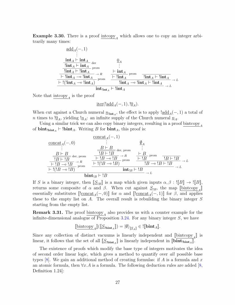
Example 3.30. There is a proof intcopyA

which allows one to copy an integer arbi-trarily many times:

addA(−, 1)...

intA ` intAder

!intA ` intA prom!intA ` !intA

( R` !intA ( !intA prom

` !(!intA ( !intA)

0A...` intA prom` !intA !intA ` !intA

( L!intA ( !intA ` !intA

( Lint!intA ` !intA

Note that intcopyA

is the proof

iter(!addA(−, 1), !0A).

When cut against a Church numeral n!intA, the effect is to apply !addA(−, 1) a total of

n times to !0A, yielding !nA: an infinite supply of the Church numeral nA.Using a similar trick we can also copy binary integers, resulting in a proof bintcopy

Aof bint!bintA ` !bintA. Writing B for bintA, this proof is:

concatA(−, 0)...

B ` Bder, prom

!B ` !B( R` !B ( !B prom

` !(!B ( !B)

concatA(−, 1)...

B ` Bder, prom

!B ` !B( R` !B ( !B prom

` !(!B ( !B)

∅A...` B prom` !B !B ` !B

( L!B ( !B ` !B

( Lint!B ` !B

( Lbint!B ` !B

If S is a binary integer, then JS!BK is a map which given inputs α, β : !JBK → !JBK,returns some composite of α and β. When cut against S!B, the map Jbintcopy

AK

essentially substitutes J!concatA(−, 0)K for α and J!concatA(−, 1)K for β, and appliesthese to the empty list on A. The overall result is rebuilding the binary integer Sstarting from the empty list.

Remark 3.31. The proof bintcopyA

also provides us with a counter example for theinfinite-dimensional analogue of Proposition 3.24. For any binary integer S, we have

JbintcopyAK(JS!bintA

K) = |∅〉JSAK ∈ !JbintAK.

Since any collection of distinct vacuums is linearly independent and JbintcopyAK is

linear, it follows that the set of all JS!bintAK is linearly independent in Jbint!bintAK.

The existence of proofs which modify the base type of integers motivates the ideaof second order linear logic, which gives a method to quantify over all possible basetypes [8]. We gain an additional method of creating formulas: if A is a formula and xan atomic formula, then ∀x.A is a formula. The following deduction rules are added [8,Definition 1.24]:

27

Γ ` A ∀RΓ ` ∀x.A

∆, A[B/x] ` C∀L

∆,∀x.A ` C

where x is not free in Γ, and A[B/x] means the formula A with all free instances of xreplaced by B. In this system, the type of integers is

int = ∀x.intx = ∀x.!(x( x) ( (x( x).

With this viewpoint, Example 3.30 shows that the sequent int ` !int is provable insecond order linear logic. We view this as perhaps the strongest argument against theintroduction of second order. Linear logic is often characterised as a ‘resource sensitive’logic, in which the copying of formulas is made explicit by use of the exponential. Theprovability of int ` !int undermines this characterisation, allowing one to hide the factthat a proof is copying by making the types in the subscript invisible. One can nolonger tell if a proof is using its inputs in a linear or nonlinear way simply by inspectingits type.

From the point of view of the Sweedler semantics, there is also a sense in whichthe copying performed by intcopy

Ais fake. The denotation of intcopy

Asends a Church

numeral JnK to the vacuum vector |∅〉JnK, and so we have

JintcopyAK(cJmK + dJnK) = c|∅〉JmK + d|∅〉JnK 6= |∅〉cJmK+dJnK.

This is similar to how if one chooses a basis {vi}i of a vector space V , there is of coursea linear map ϕ : V → V ⊗ V which naively ‘copies’, sending vi to vi ⊗ vi for all i. Butthis is superficial; while ϕ certainly copies the specific vectors vi, it fails to copy linearcombinations, as in general:

ϕ(cvi + dvj) = cvi ⊗ vi + dvj ⊗ vj 6= (cvi + dvj)⊗ (cvi + dvj).

If one is interested in differentiating proofs, then we have an additional intrinsic reasonto oppose the use of second order and proofs like bintcopy

A. Considering for example

the proof repeatA

of !bintA ` bintA, one can cut against bintcopyA

to obtain a proofof bint!bintA ` bintA, which of course cannot be differentiated; the premise no longerpossesses an exponential modality. Allowing the use of second order therefore causesany connection to differentiation to be missed. In particular, the encodings of Turingmachines in [8, 19] are incompatible with differential linear logic due to the presence ofsecond order at many intermediate steps, and it is this which motivates our developmentof a new encoding in Section 5.

28

4 Syntax of differential linear logic

So far our analysis of the differentiable structure of linear logic has been from apurely semantic perspective. It is natural to ask whether this structure can be under-stood syntactically by the addition of new deduction rules. Stated another way, theparts of the Sweedler semantics which are directly reflected by the syntax of linear logicare ⊗,⊕,Hom and the coalgebraic structure of !V . But there is additional structureon !V which is invisible from the point of view of the syntax. In this section we willdefine the syntax of differentiable linear logic, and show that it additionally reflectsboth bialgebraic structure of !V and the interactions with (k[t]/t2)∗.

Definition 4.1. The sequent calculus of differential linear logic [6, 23] consists of theusual deduction rules, together with three new rules, called coweakening, cocontractionand codereliction respectively.

Γ, !A ` Bcoder

Γ, A ` BΓ, !A ` B

coweakΓ ` B

Γ, !A ` Bcoctr

Γ, !A, !A ` B

There are new cut elimination rules, described3 in [6].

There are a number of equivalent formulations of the new rules; see [23] for anotherexample. It is easily verified that the rules given there are equivalent to the rules of Def-inition 4.1. We have chosen this presentation since it makes clear the dual relationshipbetween the rules of dereliction, weakening and contraction, and their corresponding‘co’-rules.

Remark 4.2. The new rules of Definition 4.1 may appear incongruous with our remarkson copying at the end of the previous section, since it is not difficult to devise a proof indifferential linear logic of A ` !A. From a logician’s perspective the new rules may seemparticularly offensive, given that in differential linear logic, any sequent is provable!

A ` Aweak

!Γ, A ` Acoder

Γ, A ` Ader

Γ, !A ` Acoweak

Γ ` AHowever from the perspective of computer science, the new rules are not so strange, aswe are not primarily interested in the notion of provability. Rather, our interest lies inthe computational content of the proof: its behaviour under cut elimination. In thislight, a proof of A ` !A using codereliction should not be thought of as copying A.

3The cut elimination procedure is actually defined in [6] in the language of proof nets, but thereare obvious analogues of the reductions for the sequent calculus presentation.

29

Rather, it allows us to produce instances of !A which have a linear dependence on A.This is perfectly reasonable, since the map

α 7→ |α〉0

produces an element of !JAK in a linear way from JAK.

In order to understand these new rules semantically, it will be useful to know that!V is not only a coalgebra, but a bialgebra. In brief, an (associative unital) algebra Xis a k-vector space equipped with linear maps ∇ : X ⊗X → X and η : k → X calledthe product and unit respectively and such that

X X ⊗X

X ⊗X X ⊗X ⊗X

∇

∇

∇⊗id

id⊗∇

X

X ⊗ k X ⊗X k ⊗X

∼=

id⊗η

∇∼=

η⊗id

commute4. An algebra X which is also a coalgebra is called a bialgebra [22, §3.1] if thetwo structures are compatible, in the sense that the following diagrams also commute.Here σ denotes the map a⊗ b 7→ b⊗ a.

X ⊗X X X ⊗X

X ⊗X ⊗X ⊗X X ⊗X ⊗X ⊗X

∇

∆⊗∆

∆

id⊗σ⊗id

∇⊗∇

X ⊗X k ⊗ k X ⊗X

X k X

∇

η⊗η

∼=

ε⊗ε

η

∆

ε

k X

k

η

idε

Lemma 4.3. For a vector space V , the cofree coalgebra !V is a bialgebra.

Proof. This is outlined in [22, §6.4]. Define the product ∇ : !V ⊗ !V → !V as

∇(|α1, ..., αm〉γ ⊗ |β1, ..., βn〉δ) = |α1, ..., αm, β1, ..., βn〉γ+δ,

and the unit η : k → !V as ε(1) = |∅〉0. It is easily verified that these definitions togetherwith the definitions of Section 2 equip !V with the structure of a bialgebra.

Given that the rules of contraction and weakening correspond semantically to thecoproduct and counit of !JAK, it is therefore natural that one should interpret cocon-traction and coweakening as the product and unit respectively.

4This is the categorical dual of Definition 2.3.

30

π1...Γ, !A ` B

coderΓ, A ` B

JπK(γ ⊗ a) = Jπ1K(γ ⊗ |a〉0)

π1...Γ, !A ` B

coweakΓ ` B

JπK(γ) = Jπ1K(γ ⊗ |∅〉0)

π1...Γ, !A ` B

coctrΓ, !A, !A ` B

JπK(γ ⊗ a1 ⊗ a1) = Jπ1K(γ ⊗∇(a1 ⊗ a2))

Table 4.1: Denotations of the codereliction, coweakening, and cocontraction rules.

Remark 4.4. Note that the cocontraction rule formalises the notion of linear combi-nations of proofs in the syntax. Consider the following proof:

A ` Ader

!A ` Acoctr

!A, !A ` A

which acts on vacuums by |∅〉γ ⊗ |∅〉δ 7→ γ + δ. If π1, π2 are proofs of Γ ` A, then wecan form the sum of π1 and π2 via the following proof:

π1...Γ ` A

der, prom!Γ ` !A

π2...Γ ` A

der, prom!Γ ` !A ⊗R

!Γ ` !A⊗ !A

A ` Ader

!A ` Acoctr

!A, !A ` A⊗L

!A⊗ !A ` Acut

!Γ ` ALinear combinations of proofs have a natural interpretation in terms of nondetermin-ism. For proofs π1, ..., πn of ` A, the sum Jπ1K + ... + JπnK should be thought of as asuperposition of the given proofs from which one can nondeterministically ‘choose’ [17].The connection between formal sums of proofs and nondeterminism is well studied;often this is done by explicitly adding a ‘sum’ rule [11]. We will further elaborate onthe connection between cocontraction and nondeterminism in Section 5.3.

The reasoning behind the denotation of the codereliction rule is provided by thefollowing definition, which reifies Definition 2.15 into the level of syntax.

Definition 4.5. Let π be a proof of !A ` B. Define the derivative of π, written ∂π,as the following proof:

31

π...!A ` B

coctr!A, !A ` B

coder!A,A ` B

which has denotation

J∂πK(|α1, ..., αn〉γ ⊗ a) = JπK ◦ ∇(|α1, ..., αn〉γ ⊗ |a〉0) = JπK|a, α1, ..., αn〉γ.

In particular, this means that

J∂πKnl = ∂JπK : JAK⊗ JAK→ JBK

in the sense of Definition 2.15.

32

xyy

q

z ......

tape head

machine M

Figure 5.1: A Turing machine. The internal state is q, and the machine is currentlyreading the square marked x.

5 Turing machines

The examples of proofs we have given thus far correspond to relatively elementaryfunctions such as addition and multiplication, so one could possibly form the impressionthat the computational power of linear logic is somewhat limited. Our next object ofinvestigation aims to convince the reader that this is not the case.

We briefly recall the definition of a Turing machine; for a more comprehensivetreatment, see [1, 21]. Informally speaking, a Turing machine is a computer whichpossesses a finite number of internal states, and a one dimensional ‘tape’ as memory.We adopt the convention that the tape is unbounded in both directions. The tapeis divided into individual squares each of which contains some symbol from a fixedalphabet; at any instant only one square is being read by the ‘tape head’. Dependingon the symbol on this square and the current internal state, the machine will write asymbol to the square under the tape head, possibly change the internal state, and thenmove the tape head either left or right. Formally,

Definition 5.1. A Turing machine M = (Σ, Q, δ) is a tuple where Q is a finite setof states, Σ is a finite set of symbols called the tape alphabet, and

δ : Σ×Q→ Σ×Q× {left, right}

is a function, called the transition function.

The set Σ is assumed to contain some designated blank symbol ‘ ’ which is the onlysymbol which is allowed to occur infinitely often on the tape. Often one also designates astarting state, as well as a special accept state which terminates computation if reached.

If M is a Turing machine, a Turing configuration of M is a tuple 〈S, T, q〉, whereS, T ∈ Σ∗ and q ∈ Q. This is interpreted as the instantaneous configuration of the Tur-ing machine in the following way. The string S corresponds to the non-blank contentsof the tape to the left of the tape head, including the symbol currently being scanned.The string T corresponds to a reversed copy of the contents of the tape to the right ofthe tape head, and q stores the current state of the machine. The reason for T beingreversed is a matter of convenience, as we will see in the next section.

Despite the relative simplicity of the Turing machine model, it is generally accepted[21] that any function f : Σ∗ → Σ∗ which can naturally be regarded as computable is

33

able to be computed by a Turing machine, in the sense that there exists a machine Mwhich if run on a tape which initially contains x ∈ Σ∗, then after sufficient time M willhalt with just f(w) printed on its tape.

The eventual goal of this section will be to present a method of encoding of Turingmachines in linear logic. This is based on work by Girard in [9], which encodes Turingconfigurations via a variant of second order linear logic called light linear logic. Theencoding does not use light linear logic in a crucial way, but requires second orderin many intermediate steps, making it incompatible with differentiation. Our maincontribution will be to develop an encoding which is able to be differentiated.

Remark 5.2. It is important to clarify that we are not claiming that linear logicis Turing complete - that is, able to compute the same class of functions as Turingmachines. Our encoding provides us with a proof which simulates a Turing machinefor any fixed number of computation steps, or if one is willing to use second order, aproof which can simulate a Turing machine for a variable number of steps. But this isnot the same as computing indefinitely until a certain state is reached. Indeed, sincelinear logic is strongly normalising, it is necessarily unable to simulate any computationwhich fails to halt.

Definition 5.3. Fix a finite set of states Q = {0, ..., n − 1}, and a tape alphabet5

Σ = {0, 1}, with 0 being the blank symbol. The type of Turing configurations on Ais:

TurA = !bintA ⊗ !bintA ⊗ !nboolA.

The configuration 〈S, T, q〉 is represented by the element

J〈S, T, q〉K = |∅〉JSAK ⊗ |∅〉JTAK ⊗ |∅〉JqA

K ∈ JTurAK.

Our aim is to simulate a single transition step of a given Turing machine M as aproof δstep

Aof TurB ` TurA for some formula B which depends on A, in the sense

that if said proof is cut against a Turing configuration of M at time t, the result will beequivalent under cut elimination to the Turing configuration of M at time step t + 1.This will be achieved in Theorem 5.12. Inspired by [9] and [24], our strategy will be asfollows. Let 〈Sσ, Tτ, q〉 be the (initial) configuration of the given Turing machine.

1. Decompose the binary integers Sσ and Tτ to extract their final digits, givingS, T, σ and τ . Note that σ is the symbol currently under the head, and τ is thesymbol immediately to its right.

2. Using the symbol σ together with the current state q ∈ Q, compute the newsymbol σ′, the new state q′, and the direction to move d.

5It is straightforward to modify what follows to allow larger tape alphabets. At any rate, anyTuring machine can be simulated by one whose tape alphabet is {0, 1}, so this really isn’t as restrictiveas it might seem [18].

34

σS τ T rev

qσ′S τ T rev

q′

σ′S τ T rev

q′

d = left

d = right

Figure 5.2: A single transition step of a Turing machine.

3. If d = right, append σ′τ to S. Otherwise, append τσ′ to T ; remember that thebinary integer T is the reversal of the contents of the tape to the right of the tapehead. This is summarised in Figure 5.2.

5.1 The encoding

In order to feed the current symbol into the transition function, it is necessary toextract this digit from the binary integer which represents the tape. To do this we mustdecompose a binary integer S ′ = Sσ of length l ≥ 1 into two parts S and σ, the formerbeing a bint consisting of the first l − 1 digits (the tail) and the latter being a boolcorresponding to the final digit (the head).

Throughout, let An = A& ...&A, where there are n copies of A.

Proposition 5.4. There exists a proof headA of bintA3 ` boolA which encodes thefunction JSσA3K 7→ JσAK.

Proof. The construction we will use is similar to that in [9, §2.5.3]. Let π0, π1 be the(easily constructed) proofs of A3 ` A3 whose denotations are Jπ0K(x, y, z) = (x, y, x)and Jπ1K(x, y, z) = (x, y, y) respectively. Similarly let ρ be the proof of A2 ` A3 withdenotation JρK(x, y) = (x, y, x). Define by headA the following proof:

π0...A3 ` A3

( R` A3 ( A3

prom

` !(A3 ( A3)

π1...A3 ` A3

( R` A3 ( A3

prom

` !(A3 ( A3)

ρ...

A2 ` A3A ` A

&L2

A3 ` A( L

A3 ( A3, A2 ` A( R

A3 ( A3 ` boolA( L

intA3 ` boolA( L

bintA3 ` boolA

where the rule &L2 introduces two new copies of A on the left, such that the originalcopy is at position 2 (that is, the third element of the triple).

35

We now show that JheadAK(JSσA3K) = JσAK as claimed. Recall that the denotationJSσA3K of a binary integer is a function which, given inputs α and β of type A3 ( A3

corresponding to the digits zero and one, returns some composite of α and β. The effectof the two leftmost branches of headA is to substitute Jπ0K for α and Jπ1K for β in thiscomposite, giving a linear map ϕ : JA3K→ JA3K. The rightmost branch then computesproj2 ◦ϕ ◦ JρK : JA2K→ JAK, giving a boolean.

In other words, JheadAK(JSσA3K) is the element of JboolAK given by:

(a0, a1) 7→ proj2 ◦ϕ ◦ JρK(a0, a1) = proj2 ◦ϕ(a0, a1, a0),

where ϕ is the composite of Jπ0K and Jπ1K as above. Note however that repeatedapplications of the functions JπiK only serve to update the final digit of the triple, andthus only the final copy of JπiK determines the output value. Hence the above simplifiesto

proj2 ◦ϕ(a0, a1, a0) = proj2 ◦JπσK(a0, a1, a0) = proj2(a0, a1, aσ) = aσ.

Thus JheadAK(JSσA3K) = projσ, which is indeed the boolean corresponding to σ.Lastly, we consider the special case when Sσ is the empty list. In this case, the

computation gives:proj2JρK(a0, a1) = proj2(a0, a1, a0) = a0

which captures the fact that any symbols outside the working section of the tape areassumed to be the blank symbol, 0.

Proposition 5.5. There exists a proof tailA of bintA3 ` bintA which encodes thefunction JSσA3K 7→ JSAK.

Remark. This could also be encoded as a proof of bintA2 ` bintA. However it will bemuch more convenient later if the sequents proven by headA and tailA have the samepremise, since we will need to apply them both to two copies of the same binary integer.

Proof. This is largely based on the predecessor for intA; see Example 3.12. Define π tobe the following proof:

A ` A A ` A A ` A&R

A ` A3A ` A

&L0

A3 ` A( L

A,A3 ( A3 ` A( R

A3 ( A3 ` A( A

which has denotation:JπK(ϕ)(a) = proj0(ϕ(a, a, a)).

Define ρ to be the following proof:

A ` A&L2

A3 ` Aweak

A3, !(A( A) ` A

A ` A&L2

A3 ` Aweak

A3, !(A( A) ` A

A ` A A ` A( L

A,A( A ` A&L2

A3, A( A ` Ader

A3, !(A( A) ` A&R

A3, !(A( A) ` A3

( R!(A( A) ` A3 ( A3

36

The denotation JρK is

JρK(|α1, ..., αs〉γ)(a0, a1, a2) =

(a2, a2, γa2) s = 0

(a2, a2, α1a2) s = 1

(a2, a2, 0) s > 1.

Finally, define tailA to be the following proof:

ρ...

!(A( A) ` A3 ( A3prom

!(A( A) ` !(A3 ( A3)

ρ...

!(A( A) ` A3 ( A3prom

!(A( A) ` !(A3 ( A3)

π...

A3 ( A3 ` A( A( L

!(A( A), intA3 ` A( A( L

!(A( A), !(A( A),bintA3 ` A( A2×( R

bintA3 ` bintA

Evaluated on the binary integer S, this gives a binary integer T which if fed twovacuum vectors |∅〉γ and |∅〉δ (corresponding to the digits 0, 1) will return the compositeJAK→ JAK obtained by substituting JρK|∅〉γ and JρK|∅〉δ for each copy of the digits 0 and1 respectively in S, and then finally keeping the 0th projection by the left introductionof π.

As an example, suppose that the binary integer S is 0010. Then the correspondinglinear map JAK→ JAK is

a 7→ proj0(γ ◦ δ ◦ γ ◦ γ(a, a, a))

where γ = JρK|∅〉γ, which is the morphism (a0, a1, a2) 7→ (a2, a2, γa2), and similarly for

δ. Thus, we have:

proj0(γ ◦ δ ◦ γ ◦ γ(a, a, a)) = proj0(γ ◦ δ ◦ γ(a, a, γ(a)))

= proj0(γ ◦ δ(γ(a), γ(a), γγ(a)))

= proj0(γ(γγ(a), γγ(a), δγγ(a)))

= proj0(δγγ(a), δγγ(a), γδγγ(a))

= δγγ(a).

When fed through the decomposition steps, the base type of the binary integerschanges from A3 to A. We therefore also need to modify the base type of the n-booleanrepresenting the state, in order to keep the base types compatible.

Lemma 5.6. There exists a proof nbooltypeA

of nboolA3 ` nboolA which converts an

n-boolean on A3 to the equivalent n-boolean on A; that is, it encodes JiA3K 7→ JiAK.

Proof. For i ∈ {0, ..., n − 1}, let πi be the proof of An ` A3 whose denotation is(a0, ..., an−1) 7→ (ai, ai, ai). Define nbooltype

Aas the proof:

37

π0...An ` A3 · · ·

πn−1...An ` A3

&RAn ` (A3)n

A ` A&L0

A3 ` A( L

An, nboolA3 ` A( R

nboolA3 ` nboolA

The denotation of nbooltypeA

is the function

JnbooltypeAK(ϕ)(a0, ..., an−1) = proj0 ◦ϕ((a0, a0, a0), ..., (an−1, an−1, an−1)),

and hence JnbooltypeAK(JiA3K) = JiAK.

We now move to the task of encoding the transition function δ : Σ×Q→ Σ×Q×{left, right} of a given Turing machine.

Lemma 5.7. Given any function f : {0, ..., n−1} → {0, ...,m−1}, there exists a proofF of nboolA ` mboolA which encodes f .

Proof. Let F be the following proof

A ` A &Lf(1)Am ` A ...

A ` A &Lf(n)Am ` A

&RAm ` An A ` A

( LAm, nboolA ` A

( RnboolA ` mboolA

The denotation of F is, for ϕ ∈ JnboolAK and (a0, ..., am−1) ∈ JAmK:

JF K(ϕ)(a0, ..., am−1) = ϕ(af(0), ..., af(n−1)).

In particular, this means that JF K(JiAK)(a0, ..., am−1) = proji(af(0), ..., af(n−1)) = af(i),and hence JF K(JiAK) = projf(i) = Jf(i)

AK as desired.

Proposition 5.8. Given a transition function δ : Σ×Q→ Σ×Q×{left, right}, writeδi for the component proji ◦ δ (i ∈ {0, 1, 2}). Then there exists proofs

0δtransA : boolA, nboolA ` boolA1δtransA : boolA, nboolA ` nboolA2δtransA : boolA, nboolA ` boolA

which encode δi, for i = 0, 1, 2. For δ2, we are using the convention that left = 0 andright = 1.

Proof. Given i ∈ {0, 1, 2} and and j ∈ Σ = {0, 1}, let ∆i,j be the proof obtained fromLemma 5.7 corresponding to the function δi(j,−), omitting the final ( R rule. DefineiδtransA as the following proof, where m = n if i = 1 and m = 2 otherwise:

38

∆i,0...Am, nboolA ` A

∆i,1...Am, nboolA ` A

&RAm, nboolA ` A2 A ` A

( LAm,boolA, nboolA ` A

( LboolA, nboolA ` mboolA

Then JiδtransAK is the function

JiδtransAK(ψ ⊗ ϕ)(a0, ..., am−1) = ψ(ϕ(aδi(0,0), ..., aδi(0,n−1)), ϕ(aδi(1,0), ..., aδi(1,n−1))),

and thus we have JiδtransAK(JσK⊗ JqK) = projδi(σ,q) = Jδi(σ, q)K.

Once the new state, symbol and direction have been computed, our remaining taskis to recombine the symbols with the binary integers representing the tape.

Lemma 5.9. Let W00,W01,W10,W11 be fixed binary integers, possibly empty. Thereexists a proof π(W00,W01,W10,W11) of bintA,boolA,boolA ` bintA which encodes thefunction

(S, σ, τ) 7→ SWστ .

Proof. Let E = A ( A. We give a proof corresponding to the simpler function(S, σ) 7→ SWσ, where W0,W1 are fixed binary sequences:

concatA(−,W0)...

bintA, !E, !E,A ` A

concatA(−,W1)...

bintA, !E, !E,A ` A&R

bintA, !E, !E,A ` A&A A ` A( L

bintA,boolA, !E, !E,A ` A3×( R

bintA,boolA ` bintA

where concatA is as given in Example 3.16. The required proof π(W00,W01,W10,W11)is an easy extension of this, involving two instances of the &R and ( L rules ratherthan one.

Proposition 5.10. There exist proofs 0recombA and 1recombA of

bintA, 3 boolA ` bintA

which encode the functions

(S, τ, σ, d) 7→

{S if d = 0 (left)

Sστ if d = 1 (right)and (T, τ, σ, d) 7→

{Tτσ if d = 0 (left)

T if d = 1 (right)

respectively.

Proof. Define π(−,−,−,−) as described in Lemma 5.9, omitting the final ( R rules.The desired proof 0recombA is:

39

π(∅, ∅, ∅, ∅)...

bintA, 2 boolA, !E, !E,A ` A

π(00, 10, 01, 11)...

bintA, 2 boolA, !E, !E,A ` A&R

bintA, 2 boolA, !E, !E,A ` A&A A ` A( L

bintA, 3 boolA, !E, !E,A ` A3×( R

bintA, 3 boolA ` bintA

and 1recombA is the same, with the leftmost branch replaced by π(00, 01, 10, 11) andthe second branch replaced by π(∅, ∅, ∅, ∅).

Proposition 5.11. There exist proofs

δleftA : 3 bintA3 , bintA3 , 2 nboolA3 ` bintA

δrightA

: 2 bintA3 , 2 bintA3 , 2 nboolA3 ` bintA

δstateA : bintA3 , nboolA3 ` nboolA

which, if fed the indicated number of copies of S, T and q corresponding to a Turingconfiguration, update the left part of the tape, the right part of the tape, and the staterespectively.

Proof. We simply compose (using cuts) the proofs from Propositions 5.4 through 5.10;the exact sequence of cuts is given in Figures 5.3 - 5.5. The verification that the proofsperform the desired tasks is made clear through the following informal computations.Here 〈Sσ, Tτ, q〉 is the configuration of the Turing machine at time t, and 〈S ′, T ′, q′〉 isits configuration at time t+ 1. In other words, we have δ(σ, q) = (σ′, q′, d), and

(S ′, T ′) =

{(S, Tτσ′) d = 0 (left)

(Sσ′τ, T ) d = 1 (right).

δleftA is : (Sσ)⊗3 ⊗ (Tτ)⊗ q⊗2

7−−→ S ⊗ σ⊗2 ⊗ τ ⊗ q⊗2 (tailA ⊗ head⊗3A ⊗ nbooltype⊗2

A)

7−−→ S ⊗ τ ⊗ (σ ⊗ q)⊗2 (exchange)

7−−→ S ⊗ τ ⊗ σ′ ⊗ d (id⊗2 ⊗ 0δtransA ⊗ 2

δtransA)

7−−→ S ′ (0recombA)

40

δrightA

is : (Sσ)⊗2 ⊗ (Tτ)⊗2 ⊗ q⊗2

7−−→ σ⊗2 ⊗ τ ⊗ T ⊗ q⊗2 (head⊗3A ⊗ tailA ⊗ nbooltype⊗2

A)

7−−→ T ⊗ τ ⊗ (σ ⊗ q)⊗2 (exchange)

7−−→ T ⊗ τ ⊗ σ′ ⊗ d (id⊗2 ⊗ 0δtransA ⊗ 2

δtransA)

7−−→ T ′ (1recombA)

δstateA is : (Sσ)⊗ q7−−→ σ ⊗ q (headA ⊗ nbooltype

A)

7−−→ q′. (1δtransA)

Theorem 5.12. There exists a proof δstepA

of TurA3 ` TurA which encodes a singletransition step of a given Turing machine.

Proof. The desired proof δstepA

is given in Figure 5.6.

By cutting the above construction against itself, we obtain:

Corollary 5.13. For each p ≥ 1, there exists a proof pδstepA

of TurA3p ` TurA whichencodes p transition steps of a given Turing machine.

Note that this iteration must be performed ‘by hand’ for each p; we cannot iteratefor a variable number of steps. By this we mean that it is not possible to devise a proofof intB,TurC ` TurA (for suitable types B,C) which simulates a given Turing machinefor n steps when cut against the Church numeral nB. The fundamental problem is thatiteration as in Section 3.4 only allows iteration of endomorphisms B ( B, and so thefact that our base type changes in each iteration of δstep

Amakes this impossible.

If one is willing to use second order, then iteration in the above sense becomespossible via the following proof, where Tur = ∀A.TurA:

δstepA...

TurA3 ` TurA ∀LTur ` TurA ∀RTur ` Tur

( R` Tur ( Tur prom

` !(Tur ( Tur)Tur ` Tur Tur ` Tur

( LTur ( Tur,Tur ` Tur

promintTur,Tur ` Tur

∀Lint,Tur ` Tur

41

tailA ⊗ head⊗3A ⊗ nbooltype⊗2

A...

3 bintA3 ,bintA3 , 2 nboolA3 ` bintA ⊗ bool⊗3A ⊗ nbool⊗2

A

id⊗2 ⊗ 0δtransA ⊗ 2

δtransA...

bintA,boolA, 2 (boolA, nboolA) ` bintA ⊗ bool⊗3A

exchbintA, 3 boolA, 2 nboolA ` bintA ⊗ bool⊗3

A⊗L

bintA ⊗ bool⊗3A ⊗ nbool⊗2

A ` bintA ⊗ bool⊗3A

0recombA...bintA, 3 boolA ` bintA

⊗LbintA ⊗ bool⊗3

A ` bintA

cut

3 bintA3 ,bintA3 , 2 nboolA3 ` bintA ⊗ bool⊗3A

cut3 bintA3 ,bintA3 , 2 nboolA3 ` bintA

Figure 5.3: The proof δleftA.

head⊗3A ⊗ tailA ⊗ nbooltype⊗2

A...

2 bintA3 , 2 bintA3 , 2 nboolA3 ` bool⊗3A ⊗ bintA ⊗ nbool⊗2

A

id⊗2 ⊗ 0δtransA ⊗ 2

δtransA...

bintA,boolA, 2 (boolA, nboolA) ` bintA ⊗ bool⊗3A

exch3 boolA,bintA, 2 nboolA ` bintA ⊗ bool⊗3

A⊗L

bool⊗3A ⊗ bintA ⊗ nbool⊗2

A ` bintA ⊗ bool⊗3A

1recombA...bintA, 3 boolA ` bintA

⊗LbintA ⊗ bool⊗3

A ` bintA

cut

2 bintA3 , 2 bintA3 , 2 nboolA3 ` bintA ⊗ bool⊗3A

cut2 bintA3 , 2 bintA3 , 2 nboolA3 ` bintA

Figure 5.4: The proof δrightA

.

42

tailA ⊗ nbooltypeA...

bintA3 , nboolA3 ` boolA ⊗ nboolA

1δtransA...

boolA, nboolA ` nboolA ⊗LboolA ⊗ nboolA ` nboolA

cutbintA3 , nboolA3 ` nboolA

Figure 5.5: The proof δstateA.

δleftA...3 bintA3 ,bintA3 , 2 nboolA3 ` bintA

der, prom3 !bintA3 , !bintA3 , 2 !nboolA3 ` !bintA

δrightA...

2 bintA3 , 2 bintA3 , 2 nboolA3 ` bintAder, prom

2 !bintA3 , 2 !bintA3 , 2 !nboolA3 ` !bintA

δstateA...bintA3 , nboolA3 ` nboolA

der, prom!bintA3 , !nboolA3 ` !nboolA

⊗R5 !bintA3 , 3 !bintA3 , 4 !nboolA3 ` !bintA ⊗ !bintA ⊗R

6 !bintA3 , 3 !bintA3 , 5 !nboolA3 ` TurActr

!bintA3 , !bintA3 , !nboolA3 ` TurA ⊗LTurA3 ` TurA

Figure 5.6: The proof δstepA

.

43

5.2 Copying

One aspect in which our approach differs from that given by Girard in [9] is that hepresents the type of Turing configurations without exponential modalities, as bint ⊗bint⊗ nbool.6 Our choice is made in accordance with the comments made at the endof Section 3.4; the encoding requires copying some inputs, and our understanding of thephilosophy of linear logic is that any copying should be made explicit. Nevertheless,if one does not mind the use of proofs such as bintcopy

A, it is possible to remove the

exponentials in the definition of TurA. We will now elaborate on this construction.Similarly to bintcopy

A, one can easily devise a proof nboolcopy

Aof

nbool!nboolA ` !nboolA

which copies n-booleans. One would therefore like to precompose pδstep

Awith the proof

bintcopyA3p ⊗ bintcopy

A3p ⊗ nboolcopyA3p ,

but a problem immediately arises: the base types of the binary integers would nolonger be the same as that of the n-boolean. Fortunately, the fix of this is fairlystraightforward. Let B be the type !bintA & !nboolA. For any binary integer S andany n-boolean i, there is a proof πS,i of ` B which prepares the tuple (!JSAK, !JiAK):

SA...` bintA prom` !bintA

iA...` nboolA prom` !nboolA

&R` BInformally speaking, the pair (!JSAK, !JiAK) should be thought of as an infinite supplyof copies of both the binary integer S and the n-boolean i. The idea we will use isto design variants of nboolcopy

Aand bintcopy

Ausing this tuple, and then discard the

other element by an appropriate &L introduction rule.

Lemma 5.14. There exists a proof nboolcopy∗A

of nboolB ` !nboolA which allows ann-boolean to be copied arbitrarily many times, where B = !bintA & !nboolA.

Proof. Define nboolcopy∗A

as the proof

π∅,0...` B ...

π∅,n−1...` B

&R` Bn

!nboolA ` !nboolA&L1

B ` !nboolA( L

nboolB ` !nboolA

The value of Jnboolcopy∗AK(JiBK) corresponds to projecting onto the ith component of

Bn, which is (!J∅AK, !JiAK). The &L1 rule on the rightmost branch then discards theJ!∅AK, and hence we obtain an unlimited supply of copies of JiAK as desired.

6Here bint is the second-order formula bint = ∀x.bintx, and similarly for nbool.

44

Lemma 5.15. There exists a proof bintcopy∗A

of bintB ` !bintA which copies a binaryinteger arbitrarily many times, where B = !bintA & !nboolA.

Proof. For σ ∈ {0, 1}, let ρσ denote the following proof:

concatA(−, σ)...

bintA ` bintAder

!bintA ` bintA prom!bintA ` !bintA

&L0B ` !bintA

!nboolA ` !nboolA&L1

B ` !nboolA&R

B ` B( R` B ( B prom

` !(B ( B)

Then JρσK corresponds to an infinite supply of the function JBK→ JBK given by

(!JSAK, !JqAK) 7→ (!JSσAK, !Jq

AK).

We define bintcopy∗A

as the following proof.

ρ0...` !(B ( B)

ρ1...` !(B ( B)

π∅,0...` B

!bintA3 ` !bintA3&L0

B ` !bintA3( L

B ( B ` bintA3

( LintB ` !bintA3

( LbintB ` !bintA3

We give a sketch of why this construction does in fact copy the input. Let S be somebinary integer of type bintB. Then Jbintcopy∗

AK substitutes Jρ0K and Jρ1K for the digits

0 and 1 in S respectively, and applies these to the pair (!J∅AK, !J0AK). This rebuilds Sstarting from the empty list, giving (!JSAK, !J0AK). Finally, as in Lemma 5.14 we projectonto the desired component.

By precomposing the proofs from Section 5.1 with the above proofs we obtain aproof which encodes a single step transition without exponentials:

bintcopy∗A3 ⊗ bintcopy∗

A3 ⊗ nboolcopy∗A3

...Tur∗C ` TurA3

δleftA ⊗ δrightA⊗ δstateA

...6 bintA3 , 3 bintA3 , 5 nboolA3 ` Tur∗A

der, ctr!bintA3 , !bintA3 , !nboolA3 ` Tur∗A

⊗LTurA3 ` Tur∗A

cutTur∗C ` Tur∗A

where C = !bintA3 & !nboolA3 and Tur∗A = bintA ⊗ bintA ⊗ nboolA.

45

5.3 Nondeterministic Turing machines

One variant of the standard Turing machine incorporates nondeterminism, allowingthe machine to make choices at each time step [1, §2.1.2].

Definition 5.16. A nondeterministic Turing machine M = (Σ, Q, δ0, δ1) is a vari-ant of a Turing machine which has two transition functions

δi : Σ×Q→ Σ×Q× {left, right}

rather than only one.

At any step of the computation, M will choose to use either δ0 or δ1. The runtimebehaviour of M can therefore be described by a binary integer, which specifies whichδi was used at each time step. If q0 is the starting state and qa the accept state forM , then we say that M accepts a given input string S if there exists some sequenceof choices at each time step which causes M to reach an accept state starting from〈S, ∅, q0〉.

Given our discussion of nondeterminism in Section 4, it should come as no surprisethat one can devise an encoding of nondeterministic Turing machines in differentiallinear logic. A configuration of a nondeterministic Turing machine can be thought ofas a superposition of configurations, which can be represented as the following sum:

J〈S1, T1, q1〉K + ...+ J〈Sl, Tl, ql〉K ∈ JTurAK. (∗)

Theorem 5.17. There exists a proof δstepNDA

of !TurA3 ` !TurA which encodes a singletransition step of a given non-deterministic Turing machine.

Proof. Let δstep0A, δstep1

Adenote the proofs of TurA3 ` Tur obtained from Theorem

5.12 using the transition functions δ0, δ1 respectively. Define δstepNDA

as the proof

δstep0

A...TurA3 ` TurA

der, prom!TurA3 ` !TurA

δstep1

A...TurA3 ` TurA

der, prom!TurA3 ` !TurA ⊗R

!TurA3 , !TurA3 ` !TurA ⊗ !TurActr

!TurA3 ` !TurA ⊗ !TurA

!TurA ` !TurAcoctr

!TurA, !TurA ` !TurA ⊗L!TurA ⊗ !TurA ` !TurA

cut!TurA3 ` !TurA

which has denotation

JδstepND

AK = ∇ ◦ (!Jδstep0

AK⊗ !Jδstep1

AK) ◦∆.

Let 〈S1, T1, q1〉, ..., 〈Sl, Tl, ql〉 be Turing configurations. Using the formula for the co-contraction rule in Table 4.1 (see also Lemma 4.3) we compute that the image of the

46

vacuum at the superposition (∗) under JδstepNDA

K is:

JδstepND

AK|∅〉∑l

i=1J〈Si,Ti,qi〉K

= ∇ ◦ (!Jδstep0

AK⊗ !Jδstep1

AK)(|∅〉∑l

i=1J〈Si,Ti,qi〉K ⊗ |∅〉∑li=1J〈Si,Ti,qi〉K

)= ∇

(|∅〉Jδstep0

AK(∑li=1J〈Si,Ti,qi〉K) ⊗ |∅〉Jδstep1

AK(∑li=1J〈Si,Ti,qi〉K)

)= ∇

(|∅〉∑l

i=1Jδstep0A

KJ〈Si,Ti,qi〉K ⊗ |∅〉∑li=1Jδstep1

AKJ〈Si,Ti,qi〉K

)= |∅〉∑l

i=1Jδstep0A

KJ〈Si,Ti,qi〉K+Jδstep1A

KJ〈Si,Ti,qi〉K

Remark 5.18. If X is an algebra with product ∇ and C a coalgebra with coproduct ∆,then Homk(C,A) can be equipped with the structure of an algebra via the convolutionproduct [22, §4]. For f, g ∈ Homk(C,A), their product is defined as the composite

C∆−−−−−−→ C ⊗ C f ⊗ g−−−−−−→ A⊗ A ∇−−−−−−→ A.

The above theorem therefore realises JδstepNDA

K as the convolution product of !Jδstep0AK

and !Jδstep1AK, which makes sense since J!TurAK is a bialgebra.

47

6 Polynomiality and Taylor series

One of the main uses of the exponential modality for the proofs we have studied hasbeen to produce a number of copies of a formula A via contraction and then dereliction,as in the following.

π...nA ` B

n× dern !A ` B

n− 1× ctr!A ` B

(†)

Many of the proofs we have considered so far have copied their inputs in this way,including the Church numerals, binary integers, and proofs such as repeat

A, and δstep

A.

In this section, we give a general discussion on the types of calculus one can do on suchproofs. In particular, we will show that proofs of the form (†) are polynomial in asuitable sense, and that their coalgebraic derivatives agree with the usual notion of aderivative. As a consequence, proofs of this form admit a kind of Taylor expansion [17]in terms of their coalgebraic derivatives. We will then apply this to the specific exampleof the single step Turing transition function.

The motivating example is the proof repeatA

of Example 3.17:

concatA...bintA,bintA ` bintA

2× der!bintA, !bintA ` bintA

ctr!bintA ` bintA

If S, T are fixed binary sequences, we compute:

JrepeatAKnl(aJSK + bJT K) = JconcatAK((aJSK + bJT K)⊗ (aJSK + bJT K))

= a2JSSK + ab(JST K + JTSK) + b2JTT K

The coefficients of the binary sequences in the output are polynomial functions of aand b. If we compute the coalgebraic derivative (as in Definition 2.15) of Jrepeat

AK at

aJSK + bJT K in the direction of JSK, we find that it agrees with the usual derivativeapplied to the coefficients of JSSK, JST K, JTSK and JTT K:

JrepeatAK|JSK〉aJSK+bJT K = JconcatAK((aJSK + bJT K)⊗ JSK + JSK⊗ (aJSK + bJT K))

= 2aJSSK + b(JST K + JTSK)

=∂

∂aJrepeat

AKnl(aJSK + bJT K).

We wish to generalise this construction. To this end, let A and B be formulas, n ≥ 1and suppose that π is a proof of nA ` B. We write π† for the proof (†) above.

48

Definition 6.1. For α = (α0, α1) ∈ JAK2, define a function F πα : k × k → JBK by:

F πα (a, b) = Jπ†Knl(aα0 + bα1).

If S = s1s2 . . . sn ∈ {0, 1}n is a binary integer, write αS for the tensor

αs1 ⊗ · · · ⊗ αsn ∈ JAK⊗n.

With this notation, one can write the value of F πα as

F πα (a, b) = JπK ◦ d⊗n ◦∆n−1|∅〉aα0+bα1

= JπK((aα0 + bα1)⊗n)

=∑

S∈{0,1}na|S0|b|S1|JπK(αS),

where S0 = {i | si = 0} and S1 = {i | si = 1}.Choose a basis {u1, ..., ur} of the subspace V π

α = span {JπK(αS) | S ∈ {0, 1}n} ⊆ JBK.By construction, for all a, b ∈ k we can write the value of F π

α (a, b) in terms of this basis:

F πα (a, b) =

r∑k=1

Pk(a, b)uk,

where the Pk(a, b) are functions of a and b.

Lemma 6.2. The Pk(a, b) are polynomials, and if one writes

∂i

∂ai∂j

∂bjF πα (a, b) =

r∑k=1

∂i

∂ai∂j

∂bj[Pk(a, b)]uk,

then this expression is independent as a vector in JBK of the choice of basis {u1, ..., ur}.

Proof. First assume that {JπK(αS) | S ∈ {0, 1}n} is linearly independent, and hence isa basis of V π

α . The coefficients PS corresponding to this basis are PS(a, b) = a|S0|b|S1|,which are polynomials. If not all of the JπK(αS) are linearly independent, then thePS(a, b) will instead be sums of the monomials a|S0|b|S1|, hence a polynomial. The resultthen follows for a general basis {u1, ..., ur} since changing basis is a linear operation.

Now, let {v1, ..., vr} be another basis of V πα , and let Λ be the transition matrix

between these bases, so that

uk = Λk,1v1 + ...+ Λk,rvr

for k = 1, ..., r. We therefore have:

F πα (a, b) =

r∑k=1

Pk(a, b)uk =r∑

k=1

Pk(a, b)

(r∑l=1

Λk,lvl

)=

r∑l=1

(r∑

k=1

Λk,lPk(a, b)

)vl.

49

Since differentiation is linear, it follows that

r∑l=1

∂i

∂ai∂j

∂bj

[r∑

k=1

Λk,lPk(a, b)

]vl =

r∑k=1

∂i

∂ai∂j

∂bj[Pk(a, b)]

(r∑l=1

Λk,lvl

)

=r∑

k=1

∂i

∂ai∂j

∂bj[Pk(a, b)]uk.

Proposition 6.3. Let α = (α0, α1) ∈ JAK2 and i, j ≥ 0. Then

∂i

∂ai∂j

∂bjF πα (a, b) = Jπ†K|α⊗i0 , α

⊗j1 〉aα0+bα1

. (∗)

Proof. Let Inj(X, Y ) denote the set of injective functions X → Y . By a similar com-putation to Proposition 3.5, the right hand side of (∗) is:

Jπ†K|α⊗i0 , α⊗j1 〉aα0+bα1

= JπK ◦ d⊗n ◦∆n−1(|α⊗i0 , α⊗j1 〉aα0+bα1

)

=∑f,g

JπK(Γf,g1 ⊗ · · · ⊗ Γf,gn ),

where the sum is over all f ∈ Inj([i], [n]), g ∈ Inj([j], [n]) such that im f ∩ im g = ∅ and

Γf,gs =

α0 s ∈ im f

α1 s ∈ im g

aα0 + bβ1 otherwise.

For a binary sequence S ∈ {0, 1}n, the only terms on the right hand side of (∗) whichcontribute to the coefficient of JπK(αS) are those for which im f ⊆ S0 and im g ⊆ S1.The coefficient of JπK(αS) is therefore:

| Inj([i], S0)|| Inj([j], S1)| a|S0|−ib|S1|−j =|S0|! |S1|! a|S0|−ib|S1|−j

(|S0| − i)!(|S1| − j)!,

and hence

∂i

∂ai∂j

∂bjF πα (a, b) =

∑S∈{0,1}n

|S0|!|S1|! a|S0|−ib|S1|−j

(|S0| − i)!(|S1| − j)!JπK(αS) = Jπ†K|α⊗i0 , α

⊗j1 〉aα0+bα1

.

As a consequence of Proposition 6.3, the proof π† admits a Taylor expansion in thefollowing sense.

50

Proposition 6.4. For all a, b, x, y ∈ k, we have

Jπ†K|∅〉xα0+yα1=∑i,j≥0

1

i!j!Jπ†K|α⊗i0 , α

⊗j1 〉aα0+bα1

(x− a)i(y − b)j.

Proof. Let PS(a, b) = a|S0|b|S1|, which is the coefficient of JπK(αS) in F πα (a, b). This is

a polynomial function of a and b, and thus PS admits a Taylor expansion around eachpoint (a, b) ∈ k2, as a formal identity in k[a, b, x, y]:

PS(x, y) =∑i,j≥0

1

i!j!

∂i

∂ai∂j

∂bj[PS(a, b)](x− a)i(y − b)j.

Hence we have

Jπ†K|∅〉xα0+yα1=

∑S∈{0,1}n

PS(x, y)JπK(αS)

=∑

S∈{0,1}n

∑i,j≥0

1

i!j!

∂i

∂ai∂j

∂bj[PS(a, b)](x− a)i(y − b)jJπK(αS)

=∑i,j≥0

∑S∈{0,1}n

1

i!j!

∂i

∂ai∂j

∂bj[PS(a, b)](x− a)i(y − b)jJπK(αS)

=∑i,j≥0

∑S∈{0,1}n

1

i!j!Jπ†K|α⊗i0 , α

⊗j1 〉aα0+bα1

(x− a)i(y − b)j

by Proposition 6.3.

In the particular case where x = b = 0 and y = a = 1, this simplifies to

Jπ†K|∅〉α0=∑i,j≥0

(−1)j

i!j!Jπ†K|α⊗i0 , α

⊗j1 〉α1

.

A remarkable special case is where α1 = 0, which gives

Jπ†K|∅〉α0=∑i≥0

1

i!Jπ†K|α⊗i0 〉0.

Thus, for proofs of the form π†, the value of Jπ†Knl is determined by the values of Jπ†Kon kets based at zero.

Example 6.5. Consider π† = repeatA

and α0 = JSK, α1 = JT K. We compute:∑i,j≥0

(−1)i

i!j!Jrepeat

AK|JSK⊗i, JT K⊗j〉JT K

= JrepeatAK(|∅〉JT K − |JT K〉JT K + |JT K, JT K〉JT K

+ |JSK〉JT K − |JSK, JT K〉JT K + |JSK, JSK〉JT K)

= JTT K− 2JTT K + JTT K + (JST K + JTSK)− (JST K + JTSK) + JSSK= Jrepeat

AK|∅〉JSK.

51

A generalisation of the limit calculation of Example 3.17 also applies to π†.

Proposition 6.6. When k = C, we have

Jπ†K|α1〉α0= lim

h→0

Jπ†K|∅〉α0+hα1− Jπ†K|∅〉α0

h,

where the limit is taken in the finite-dimensional span of all JπK(αS), S ∈ {0, 1}∗.

Proof. We compute:

limh→0

1

h

(Jπ†K|∅〉α0+hα1

− Jπ†K|∅〉α0

)= lim

h→0

1

h

∑S∈{0,1}nS 6=0n

h|S1|JπK(αS)

=n∑i=1

JπK(α⊗i−10 ⊗ α1 ⊗ α⊗n−i0 )

= Jπ†K|α1〉α0.

Remark 6.7. Note that we know of at least one example of a proof which is not of theform π† for which a similar calculation applies, namely multA from Example 3.11. Fromthe example, one can see that it is really the fact that multA depends in a polynomialway on its inputs that makes such limiting calculations possible. It is our belief thatin fact all proofs are polynomial in an appropriate sense, but we have been unable toprove this assertion.

We devote the remainder of this section towards a discussion of the derivative ofthe single step transition function of a Turing machine. Our purpose is to give a simpleexample where the derivative of a proof has a clear computational meaning. WithΣ = {0, 1} and Q = {0, ..., n− 1}, let δ : Σ×Q→ Σ×Q× {0, 1} be a fixed transitionfunction. As above, write δleft†A for the proof:

δleftA...3 bintA3 ,bintA3 , 2 nboolA3 ` bintA

der3 !bintA3 , !bintA3 , 2 !nboolA3 ` bintA

ctr!bintA3 , !bintA3 , !nboolA3 ` bintA

and similarly for δright†A

and δstate†A. By the above, one can write the single steptransition of a Turing machines in terms of vacuums at polynomial functions of itsinputs. Suppose that S0, S1, T ∈ Σ∗, σ0, σ1, τ ∈ Σ, q ∈ Q, a, b ∈ k, and write(σ′i, q

′i, di) = δ(σi, q) for i = 0, 1.

52

Proposition 6.8. The single step transition evaluates as:

JδstepAK(|∅〉aJS0σ0K+bJS1σ1K ⊗ |∅〉JTτK ⊗ |∅〉JqK) = |∅〉α ⊗ |∅〉β ⊗ |∅〉γ,

with

α = (a+ b)(aδd0=0 + bδd1=0)(aJS0K + bJS1K)+ (aδd0=1 + bδd1=1)(a2JS0σ

′0τK + abJS0σ

′1τK + abJS1σ

′0τK + b2JS1σ

′1τK).

β = (a+ b)(aδd0=1 + bδd1=1)JT K + (aδd0=0 + bδd1=0)(aJTτσ′0K + bJTτσ′1K)

γ = aJq′0K + bJq′1K,

where δ is the Kronecker delta.

Proof. See Appendix A.

Remark 6.9. While one is tempted to say that the formulas for α, β, γ are simply anondeterministic sum, the full picture is more complicated. Many of the terms appearto have no obvious classical meaning. For instance

abδd1=0JTτσ′0K

has used σ0 to produce the new state, but σ1 to produce the direction to move!It is natural to ask whether this variant of nondeterminism has any intrinsic com-

putational meaning. Assume that 0 ≤ ai ≤ 1 and∑

i ai = 1, and interpret a1, ..., as asbeing a probability distribution over states α1, ..., αs. The essential difference betweenclassical nondeterminism and the above seems to be that classical nondeterminism hasits roots in copying values∑

i

ai|∅〉αi∆7−−−−→

∑i

ai|∅〉αi ⊗ |∅〉αi ,

in which the superposition of values simply refers to our lack of knowledge about the‘true’ computational state. In contrast, the variant of nondeterminism in Proposition6.8 corresponds to copying the distribution itself

|∅〉∑i aiαi

∆7−−−−→ |∅〉∑i aiαi

⊗ |∅〉∑i aiαi

,

in which the state of the machine is genuinely undetermined until the distribution issampled from by a dereliction. We believe this form of nondeterminism deserves furtherstudy.

Let us now examine the computational content of Proposition 6.8 in the special case

53

where σ = σ0 = σ1. The polynomial for the right hand part of the tape is

Jδright†AK(|∅〉aJS0σK+bJS1σK ⊗ |∅〉JTτK ⊗ |∅〉JqK)

= JδrightAK((aJS0σK + bJS1σK)⊗2 ⊗ JTτK⊗2 ⊗ JqK⊗2)

= a2JδrightAK(JS0σK⊗ JS0σK⊗ JTτK⊗2 ⊗ JqK⊗2)+

abJδrightAK(JS0σK⊗ JS1σK⊗ JTτK⊗2 ⊗ JqK⊗2)+

baJδrightAK(JS1σK⊗ JS0σK⊗ JTτK⊗2 ⊗ JqK⊗2)+

b2JδrightAK(JS1σK⊗ JS1σK⊗ JTτK⊗2 ⊗ JqK⊗2)

= (a+ b)2(δd=0JTτσ′K + δd=1JT K).

Observe that the polynomial coefficient (a + b)2 is symmetric in a and b. This is noaccident, and in fact one can restate this fact in terms of the vanishing of a derivativeas follows. Note that we have a canonical isomorphism of k-algebras

k[a, b]∼=−−−−→ k[x, y]

via x = a + b, y = a− b, and moreover for f ∈ k[a, b] we have ∂∂yf = 0 if and only if f

is a polynomial in x. Note that

∂f

∂y=∂f

∂a

∂a

∂y+∂f

∂b

∂b

∂y=

1

2

(∂f

∂x− ∂f

∂y

).

So the fact that evaluation by δrightA

gives a polynomial in a + b is exactly capturedby the vanishing of the following coalgebraic derivative.

Proposition 6.10. Jδright†AK(|JS0σK− JS1σK〉aJS0σK+bJS1σK ⊗ |∅〉JTτK ⊗ |∅〉JqK) = 0.

Proof. Simply note that applying headA to JS0σK− JS1σK yields JσK− JσK = 0.

This is precisely the type of computational content one would hope to be visible inthe derivatives, namely the fact that the right part of the tape does not depend on S0

versus S1 after one time step. Moreover, this fact appears to be independent of theminor details of the encoding.

54

A Polynomiality of Turing machines

In this appendix, we compute the value of JδstepAK on

Ψ = |∅〉aJS0σ0K+bJS1σ1K ⊗ |∅〉JTτK ⊗ |∅〉JqK.

Note thatJδstep

AK(Ψ) = |∅〉Jδleft†AK(Ψ) ⊗ |∅〉Jδright†

AK(Ψ) ⊗ |∅〉Jδstate†AK(Ψ),

and so the problem reduces to computing the values of each of Jδleft†AK, Jδright†AK, and

Jδstate†AK on Ψ. By similar computations to those in Proposition 5.11, we find that forall i, j, k ∈ {0, 1} we have

• JδleftAK(JSiσiK⊗ JSjσjK⊗ JSkσkK⊗ JTτK⊗ JqK⊗2) = δdk=0JSiK + δdk=1JSiσ′jτK,

• JδrightAK(JSjσjK⊗ JSkσkK⊗ JTτK⊗2 ⊗ JqK⊗2) = δdk=0JTτσ′jK + δdk=1JT K,

• JδstateAK(JSiσiKJqK) = Jq′iK,

where δ on the right is the Kronecker delta. Using this, we compute

Jδleft†AK(Ψ) = a3JδleftAK(JS0σ0K⊗ JS0σ0K⊗ JS0σ0K⊗ JTτK⊗ JqK⊗2)

+ a2b(JδleftAK(JS0σ0K⊗ JS0σ0K⊗ JS1σ1K⊗ JTτK⊗ JqK⊗2)

+ JδleftAK(JS0σ0K⊗ JS1σ1K⊗ JS0σ0K⊗ JTτK⊗ JqK⊗2)

+ JδleftAK(JS1σ1K⊗ JS0σ0K⊗ JS0σ0K⊗ JTτK⊗ JqK⊗2))

+ ab2(JδleftAK(JS0σ0K⊗ JS1σ1K⊗ JS1σ1K⊗ JTτK⊗ JqK⊗2)

+ JδleftAK(JS1σ1K⊗ JS1σ1K⊗ JS0σ0K⊗ JTτK⊗ JqK⊗2)

+ JδleftAK(JS1σ1K⊗ JS0σ0K⊗ JS1σ1K⊗ JTτK⊗ JqK⊗2))

+ b3JδleftAK(JS1σ1K⊗ JS1σ1K⊗ JS1σ1K⊗ JTτK⊗ JqK⊗2)

= a3(δd0=0JS0K + δd0=1JS0σ′0τK) + a2b(δd1=0JS0K + δd1=1JS0σ

′0τK

+ δd0=0JS0K + δd0=1JS0σ′1τK + δd0=0JS1K + δd0=1JS1σ

′0τK)

+ ab2(δd1=0JS0K + δd1=1JS0σ′1τK + δd0=0JS1K + δd0=1JS1σ

′1τK

+ δd1=0JS1K + δd1=1JS1σ′0τK) + b3(δd1=0JS1K + δd1=1JS1σ

′1τK)

= (a+ b)(aδd0=0 + bδd1=0)(aJS0K + bJS1K)+ (aδd0=1 + bδd1=1)(a2JS0σ

′0τK + abJS0σ

′1τK + abJS1σ

′0τK + b2JS1σ

′1τK).

55

Jδright†AK(Ψ) = a2Jδright

AK(JS0σ0K⊗ JS0σ0K⊗ JTτK⊗2 ⊗ JqK⊗2)

+ ab(JδrightAK(JS0σ0K⊗ JS1σ1K⊗ JTτK⊗2 ⊗ JqK⊗2)

+ JδrightAK(JS1σ1K⊗ JS0σ0K⊗ JTτK⊗2 ⊗ JqK⊗2))

+ b2JδrightAK(JS1σ1K⊗ JS1σ1K⊗ JTτK⊗2 ⊗ JqK⊗2)

= a2(δd0=0JTτσ′0K + δd0=1JT K)

+ ab(δd1=0JTτσ′0K + δd1=1JT K + δd0=0JTτσ′1K + δd0=1JT K)

+ b2(δd1=0JTτσ′1K + δd1=1JT K)

= (a+ b)(aδd0=1 + bδd1=1)JT K + (aδd0=0 + bδd1=0)(aJTτσ′0K + bJTτσ′1K).

Jδstate†AK(Ψ) = aJδstateAK(JS0σ0K⊗ JqK) + bJδstateAK(JS1σ1K⊗ JqK)= aJq′0K + bJq′1K.

56

References

[1] S. Arora, B. Barak, Computational complexity: a modern approach, CambridgeUniversity Press, New York, 2009.

[2] M. Barr, Coalgebras over a commutative ring, Journal of Algebra 32 (1974), 600–610.

[3] , *-Autonomous categories and linear logic, Mathematical Structures inComputer Science 1 (1991), 159–178.

[4] A. Blass, A game semantics for linear logic, Annals of Pure and Applied Logic 56(1992), 183–220.

[5] P. de la Harpe, Topics in geometric group theory, The University of Chicago Press,2000.

[6] T. Ehrhard, An introduction to differential linear logic: proof-nets, models andantiderivatives, arXiv preprint [arXiv: 1606.01642] (2016).

[7] V. Drensky, E. Formanek, Polynomial identity rings, Birkhauser Basel, 2004.

[8] J.-Y. Girard, Linear logic, Theoretical Computer Science 50 (1987), 1–101.

[9] , Light linear logic, Information and Computation 143 (1998), 175–204.

[10] D. Eisenbud, J. Harris, The geometry of schemes, Springer-Verlag, New York, 2000.

[11] F. Maurel, Nondeterministic light logics and NP-time, vol. 2701, 2003, pp. 241–255.

[12] P.A. Mellies, Categorical semantics of linear logic, in Interactive models of com-putation and program behaviour, vol. 27, 2009.

[13] D. Murfet, Logic and linear algebra: an introduction, arXiv preprint [arXiv:1701.01285] (2014).

[14] , On Sweedler’s cofree cocommutative coalgebra, J. Pure and Applied Alge-bra [arXiv: 1701.01285] 219 (2015), 5289–5304.

[15] J. Clift, D. Murfet, Cofree coalgebras and differentiable linear logic, arXiv preprint[arXiv: 1701.01285] (2017).

[16] P. Etingof, S. Gelaki, D. Nikshych, V. Ostrik, Tensor categories, vol. 205, AmericanMathematical Society, Providence, Rhode Island, 2015.

[17] T. Ehrhard, L. Regnier, The differential lambda-calculus, Theoretical ComputerScience 309 (2003), 1–41.

57

[18] Y. Rogozhin, Small universal Turing machines, Theoretical Computer Science 168(1996), 215–240.

[19] L. Roversi, A P-time completeness proof for light logics, in Proceedings of CSL,1999, pp. 469–483.

[20] R. Blute, J. Cockett, R. Seely, Differential categories, Mathematical Structures inComputer Science 16 (2006), 1049–1083.

[21] M. Sipser, Introduction to the theory of computation, Thomson Course Technology,Boston, 2006.

[22] M. Sweedler, Hopf algebras, W.A. Benjamin, New York, 1969.

[23] R. Blute, T. Ehrhard, C. Tasson, A convenient differential category, arXiV preprint[arXiv:1006.3140] (2010).

[24] H. Mairson, K. Terui, On the computational complexity of cut-elimination in linearlogic, in Proceedings of ICTCS 2003, vol. 2841, Springer, 2003, pp. 23–36.

[25] K. Terui, Light logic and polynomial time computation, Ph.D. thesis, Keio Univer-sity, 2002.

58

Notation

Σ∗ The set of (finite) words over an alphabet Σ

[n] The set {1, ..., n}

∆ Coproduct of a coalgebra, C → C ⊗ C, 2.3

ε Counit of a coalgebra, C → k, 2.3

G(C) Set of grouplike elements of a coalgebra C, 2.5

Pγ(C) Set of primitive elements over γ of a coalgebra C, 2.5

!V Cofree cocommutative coalgebra generated by V , 2.8

|α1, ..., αn〉γ Element of !V : the equivalence class of α1 ⊗ ... ⊗ αn in the copy ofSym(V ) associated to γ, 2.10

|∅〉γ Vacuum vector (empty ket) at γ, 2.10

d Dereliction map, !V → V , 2.8

promϕ Promotion of ϕ : !V → W to a coalgebra morphism Φ : !V → !W , 2.8

J·K Denotation of a formula or proof, 2.11, 2.12

JπKnl Nonlinear map induced by a proof π of !A ` B, 2.13

∂γJπK Derivative of JπK at γ, 2.15

∂π Derivative of a proof π of !A ` B, 4.5

∇ Product of an algebra, C → C ⊗ C, 4.1

η Unit of an algebra, C → k, 4.1

〈S, T, q〉 Configuration of a Turing machine, 5.1

δ Transition function of a Turing machine, 5.1

π† The proof of !A ` B obtained from π : nA ` B by appending n derelic-tions then n− 1 contractions, 6.1

F πα The nonlinear function F π

α (a, b) = Jπ†Knl(aα0 + bα1), k2 → JBK, 6.1

αS For S ∈ {0, 1}n, the tensor αs1 ⊗ ...⊗ αsn , 6.1

nA n copies of a formula A

59

E The type A( A

boolA Type of booleans, 3.1A2 ( A

nboolA Type of n-booleans, 3.2An ( A, n ≥ 2

intA Type of integers, 3.3!(A( A) ( (A( A)

bintA Type of binary integers, 3.13!(A( A) ( (!(A( A) ( (A( A))

TurA Type of Turing configurations, 5.3!bintA ⊗ !bintA ⊗ !nboolA

iA Church numeral or n-boolean corresponding to i ∈ N, 3.3, 3.2` int or ` nbool

SA Proof corresponding to a binary integer S ∈ {0, 1}∗, 3.13` bint

compA

Composition of two endomorphisms, 3.4A,A( A,A( A ` A

addA Addition of two integers, 3.10intA, intA ` intA

multA Multiplication of two integers, 3.11!intA, intA ` intA

predA

Predecessor of an integer, 3.12intA2 ` intA

concatA Concatenation of binary integers, 3.16bint,bint ` bintA

repeatA

Repetition of binary integers, 3.17!bint ` bintA

iter(π, ρ) Iteration of the proof π evaluated on ρ, 3.28intA ` A

intcopyA

Copies an integer arbitrarily many times, 3.30int!int ` !intA

headA Returns the final digit of a binary integer, 5.4bintA3 ` boolA

60

tailA Deletes the final digit of a binary integer, 5.5bintA3 ` bintA

booltypeA

Converts the base type of an n-boolean, 5.6

nboolA3 ` nboolA

iδtransA Computes the transition function of a Turing machine, 5.8

bintA, nboolA ` mboolA

irecombA Recombines the tape binary integers, 5.10bintA,boolA,boolA ` bintA

δleftA Updates the left part of the tape of a Turing machine, 5.113 bintA3 ,bintA3 , 2 nboolA3 ` bintA

δrightA

Updates the right part of the tape of a Turing machine, 5.112 bintA3 , 2 bintA3 , 2 nboolA3 ` bintA

δstateA Updates the state of a Turing machine, 5.11bintA3 , nboolA3 ` nboolA

δstepA

Simulates a transition step of a Turing machine, 5.12TurA3 ` TurA

δstepNDA

Simulates a transition step of a nondeterministic Turing machine, 5.17!TurA3 ` !TurA

61