arX

iv:h

ep-p

h/07

0309

2v1

8 M

ar 2

007

hep-ph/0703092HRI-P-07-03-001

OUTP 0703P

Turbulent Supernova Shock Waves and the Sterile Neutrino Signature

in Megaton Water Detectors

Sandhya Choubey1∗, N. P. Harries2†, G.G. Ross2‡

1Harish-Chandra Research Institute,

Chhatnag Road, Jhunsi, Allahabad 211 019, INDIA

2The Rudolf Peierls Centre for Theoretical Physics,

University of Oxford, 1 Keble Road, Oxford, OX1 3NP, UK

Abstract

The signatures of sterile neutrinos in the supernova neutrino signal in megaton water Cerenkov detectorsare studied. Time dependent modulation of the neutrino signal emerging from the sharp changes in theoscillation probability due to shock waves is shown to be a smoking gun for the existence of sterile neutrinos.These modulations and indeed the entire neutrino oscillation signal is found to be different for the casewith just three active neutrinos and the cases where there are additional sterile species mixed with theactive neutrinos. The effect of turbulence is taken into account and it is found that the effect of the shockwaves, while modifed, remain significant and measurable. Supernova neutrino signals in water detectors cantherefore give unambiguous proof for the existence of sterile neutrinos, the sensitivity extending beyond thatfor terrestial neutrino experiments. In addition the time dependent modulations in the signal due to shockwaves can be used to trace the evolution of the shock wave inside the supernova.

∗email: sandhya@mri.ernet.in†email: n.harries1@physics.ox.ac.uk‡email: g.ross1@physics.ox.ac.uk

1

1 Introduction

The detection of neutrinos from SN1987A in the Large Megallenic Cloud remains a major landmark in neutrinophysics and astrophysics. The 11 events detected in Kamiokande [1] and 8 events in IMB [2] stimulated aplethora of research papers exploring both type-II supernova dynamics and neutrino properties [3]. A supernovaexplosion within our own galaxy will generate tens of thousands of events in the currently running and proposedneutrino detectors and hence is expected to significantly improve our understanding of the type-II supernovaexplosion mechanism on one hand and neutrino physics on the other.

Our knowledge on the pattern of neutrino mass and mixing has seen tremendous improvement from theresults of a series of outstanding experiments with solar [4], reactor [5, 6], atmospheric [7] and accelerator[8, 9] neutrinos. The existence of neutrino flavor mixing and oscillations have been established beyond doubt.The 3σ range for the mixing parameters governing solar neutrino oscillations is 1 ∆m2

21 = (7.2 − 9.2) × 10−5

eV2 and sin2 θ12 = 0.25 − 0.39 [10], while the atmospheric neutrino oscillation parameters are restricted to bewithin the range ∆m2

31 = 2.0 − 3.2 × 10−3 and 0.34 < sin2θ23 < 0.68 with sin2 2θ23 < 0.9 [10]. However,the last mixing angle θ13 remains unmeasured, although we do know that it must be small. The current 3σupper bound on the allowed values for this parameter is sin2 θ13 < 0.044 [10]. If θ13 is close to the upperbound it opens up the possibility of observing CP violation in the lepton sector – the CP phase δCP being thesecond missing link in our measurement of the neutrino mass matrix. Also still unknown is sgn(∆m2

31), whichdetermines the ordering of the neutrino mass spectrum, aka the neutrino mass hierarchy. The case ∆m2

31 > 0corresponds to the normal mass hierarchy (N3) while ∆m2

31 < 0 corresponds to the inverted mass hierarchy(I3).2 A number of suggestions have been put forward to determine these three unmeasured parameters. Theseinclude the measurement of antineutrinos from reactors with detector set-up aiming to achieve sub-percent levelin systematic uncertainties [11], using intense conventional νµ beams produced by decay of accelerated pions[12, 13], using νe beams produced by decay of accelerated radioactive ions stored in rings (“Beta-Beams”) [14]and using νe and νµ beams produced by decay of accelerated muons stored in rings (“Neutrino Factory”) [15].Most of these proposed experiments are expected to be very expensive as well as technologically challenging.

In principle, information on two of the three parameters mentioned above can be obtained by observing theneutrinos released from a galactic supernova. Detailed studies on the potential of using supernova neutrinosto unravel the mass hierarchy and θ13 have been performed in the context of water Cerenkov detectors in[16] and (large) scintillator detectors in [17]. It was shown that the neutrino telescope, IceCube, even thoughdesigned to observe ultra high energy neutrinos, could be used very effectively to detect low energy supernovaneutrinos [18, 19]. Most studies on determining of sgn(∆m2

31) and θ13 with supernova neutrinos depend onthe hierarchy between the average energies of νe, νe and νx, where νx stands for νµ, νµ, ντ , or ντ . Howeverthe most recent supernova models which take into account the full range of the significant neutrino transportprocesses, predict very little difference between the average energies of νe and νx [20]. At the same time theyalso seem to be inconsistent with equi-partition of energy between the different neutrino species, an assumptionof all earlier papers on supernova neutrinos [21]. In a nutshell, model uncertainties in the supernova parameterscould washout the oscillation effects and render this method of hierarchy and θ13 determination useless.

Less model dependent signatures of sgn(∆m231) and θ13 can be seen through the “shock effects” in the

supernova neutrino signal in large detectors [19, 22, 23, 24, 25, 26]. The steep density profile at the shockfront results in a drastic change in the oscillation probability and hence can yield information on the neutrinoproperties (sgn(∆m2

31) and θ13) despite the uncertainties associated with the supernova dynamics and neutrinotransport. However it is also expected that the shock, as it moves outward, will leave behind a turbulence in thedensity profile of the supernova matter. Early studies indicated that this could severely obscure the oscillationsignals due to the shock wave [27]. Here we reexamine this in detail following a recent analysis of the the effectof turbulence in [28]. In this the nature of the shock plays an important role. In addition to the initial forwardshock it is expected from supernova simulations that a reverse shock is formed [25]. We find that the effects ofthe reverse shock are wiped out by turbulence but that the effects of the forward shock, while changed, are stillsignificant and leave a clear signal of the resonant oscillation.

Another important question in neutrino physics is how many (if any) sterile neutrino species there are. The

1We adopt the convention in which m2

ij = m2

i − m2

j .2Note that the same notation is used even when the neutrino mass spectrum is quasi-degenerate since the NH and IH terms

here refer only to the sgn(∆m2

31).

2

first, and so far the only, experimental evidence which requires the presence of sterile neutrinos comes from theLSND experiment [29]. While the so-called 2+2 and 3+1 scenarios involving only 1 sterile neutrino [30] arenow comprehensively disfavored by the global neutrino data, the 3+2 scheme with 2 sterile neutrinos mildlymixed with the 3 active neutrinos has a more acceptable fit to all data including LSND [31] although the valueof the associated LSND mixing angle is still problematic [32]. The LSND result will be checked by the on-goingMiniBOONE experiment [33] which is expected to give the final verdict at least on the oscillation interpretationof the LSND data. However, even though MiniBOONE should refute the LSND result, it will still leave ampleroom for the existence of extra sterile neutrinos with mixing angles below its sensitivity limit. We show thatmeasurement of supernovae oscillation effects provide a much more sensitive probe for sterile neutrinos andanalyze in detail the signal that results assuming the 3+2 LSND scenario.

In [19] we analyzed the signature in the IceCube detector of neutrino oscillation occuring within a galacticsupernova, taking shock effects into account and assuming that the 3+2 mixing scheme was true. We consideredall possible neutrino mass spectrum with 3 active and 2 sterile neutrinos and showed that IceCube coulddistinguish between these different mass spectra. We also showed how well IceCube could distinguish the casewhere there were only 3 active neutrinos from the ones where there are 2 additional sterile neutrinos. Inthis paper we repeat this analysis for the case in megaton water Cerenkov detectors, including the effect ofturbulence. Water Cerenkov detectors have a good energy resolution and allow for the reconstruction of theenergy of the incoming neutrinos. Thus, for such detectors, we will have information on both the time as wellas the energy of the arriving supernova neutrinos. We calculate the number of supernova νe events in a genericmegaton water Cerenkov detector. We calculate this expected signal first for the case of three active neutrinosand then for the case with two extra sterile species. We show that the presence of sterile neutrinos changes thetime evolution of the average energy as well as the flux of the supernova neutrinos. Therefore, this can be usedto indicate the presence of sterile neutrino and also to distinguish between the different possible mass spectrumscenarios. The effect of the shock is shown to be significant on the resultant signal. We discuss the issue ofturbulence and take into account the turbulence due to the passage of shock.

The paper is organized as follows. We begin in Section 2 with a brief review of neutrino oscillations insidesupernova. We discuss the effect of the shock wave on the oscillation probability, with and without the turbulencecaused by the passage of shock. The impact on the neutrino oscillation probability by the turbulence in thematter density behind the shock is clearly outlined. In Section 3 we discuss the neutrino spectrum producedinside the supernova and their mode of detection in water Cerenkov experiments. In section 4 we present ourresults and discuss the implications in Section 5. We end with our conclusions in Section 6.

2 Neutrino Oscillations Inside the Supernova

When neutrinos propagate in matter, they pick up an extra potential energy induced by their charged currentand neutral current interactions with the ambient matter [34, 35, 36]. Since normal matter only containselectrons, only νe and νe undergo both charged as well as neutral current interactions, while the other 4 activeneutrino species have only neutral current interactions. The evolution equation of (anti)neutrinos inside thesupernova can be written in the flavor basis as

H =1

2E(UM2U † + A) , (1)

where U is a unitary matrix and is defined by |νi〉 =∑

α Uiα|να〉, νi and να being the mass and flavor eigenstatesrespectively. For the case where we consider two extra sterile neutrinos, i = 1−5 and α=e, µ, τ , s1 or s2, wheres1 and s2 are the two sterile neutrinos. The matrices M2 and A are given respectively by

M2 = Diag(m21, m

22, m

23, m

24, m

25) , (2)

A = Diag(A1, 0, 0, A2, A2) , (3)

A1 = ACC = ±√

2GF ρNAYe × 2E , (4)

A2 = −ANC = ±√

2GF ρNA(1 − Ye) × E . (5)

3

The quantities ACC and ANC are the matter induced charged current and neutral current potentials respectivelyand depend on the Fermi constant GF , matter density ρ, Avagadro number NA, electron fraction Ye and energyof the neutrino E. The “+” (“−”) sign in Eqs. (4) and (5) corresponds to neutrinos (antineutrinos).

The corresponding expressions for the three neutrino framework follows simply by dropping the extra 2states due to the sterile components. Note that we have recast the matter induced mass matrix such that theneutral current part ANC , which appears for all the three active flavors, is filtered out from the first threediagonal terms and hence it appears as a negative matter potential for the sterile states which do not have anyweak interactions. Therefore, for the three active neutrino set-up the mass matrix is

M2 = Diag(m21, m

22, m

23) , (6)

A = Diag(A1, 0, 0) . (7)

The mixing matrix U is given in terms of mixing angles and CP-violating phases. If CP conservation is assumedthe mixing matrix takes the form

U =

n∏

B>A

n−1∏

A=1

RAB(θAB) , (8)

where n = 3 for only three active neutrinos and n = 5 when two additional sterile neutrinos are present andRAB is an n × n rotation matrix about the AB plane.

Assuming that all phases get averaged out, the survival probability Pee of νe after they have propagatedthrough the supernova matter can be written as3

Pee =∑

i,j

|Uej |2|Umei |2Pij , (9)

where, Pij = |〈νj |νmi 〉|2 and Uei and Um

ei are the elements of the mixing matrix in vacuum and inside matterrespectively and |〈νj |νm

i 〉|2 is the effective “level crossing” probability that an antineutrino state created as |νmi 〉

inside the supernova core emerges as the state |νi〉 in vacuum. Largest flavor conversions occur at the resonancedensities. For two flavor oscillations, the resonance condition for antineutrinos involving only either the νe orthe sterile states is given by [35]

|Ak| = (−1)k∆m2ji cos 2θij , (10)

where k could be either 1 or 2, ∆m2ji ≡ m2

j − m2i is the mass squared difference and θij is the mixing angle

between the two states in vacuum. Note in Eq. (10), we included the sign factor (−1)k in order to take intoaccount the fact that ACC < 0 and ANC > 0 for the antineutrinos. Since ACC < 0 (ANC > 0), the conditionof resonance is satisfied only when the relevant ∆m2

ji < 0 (∆m2ji > 0). For the resonance between the νe and

sterile states one must satisfy the condition

ACC − ANC = ∆m2ji cos 2θij , (11)

which is satisfied for antineutrinos when ∆m2ji < 0 since ACC > ANC .

The probability of level crossing from one mass eigenstate to another is predominantly non-zero only atthe resonance. In the approximation that the individual two flavor resonances are far apart, the effectivelevel crossing probability can be written in terms of the individual two flavor “flip probability” Pij . The “flipprobability” between the two mass eigenstates used in this paper is given by [38]

Pij =exp(−γ sin2 θij) − exp(−γ)

1 − exp(−γ), (12)

γ = π∆m2

ji

E

∣

∣

∣

∣

d lnA

dr

∣

∣

∣

∣

−1

r=rmva

, (13)

3Since we are interested in the detection of supernova neutrino in water Cerenkov detectors where the largest number of eventsare expected through the capture of νe by protons, we will mostly refer to the survival probability of νe (Pee) in this section.However, similar expressions are valid even for the νe survival probability.

4

where A is ACC , ANC or ACC − ANC depending on the states involved in the resonance, rmva is the positionof the maximum violation of adiabaticity (mva) [37] and is defined as

A(rmva) = ∆m2ji . (14)

One can see from the above equations that Pij and hence the transition probability depends crucially both onthe mixing angle as well as on the density gradient. If for given ∆m2

ji and θij , the density gradient is small

enough so that γ ≫ 1 and γ sin2 θ ≫ 1, Pij ≃ 0 and the transition is called adiabatic. On the other hand,if the density gradient is very large or θij is very small, then Pij ≃ cos2 θij . In this case we have an extremenon-adiabatic transition. For all intermediate values of the density gradient and θij , Pij ranges between [0-1].

2.1 Neutrino Oscillations with Static Density Profile

Three active neutrinos only: As discussed above, in the three neutrino framework we have two possibilitiesfor the neutrino mass spectrum, the normal (∆m2

31 > 0) and inverted (∆m231 < 0) hierarchy. We will call them

N3 and I3 cases respectively. Also, since here we have 2 independent ∆m2ji, we can have 2 resonances and hence

the final level crossing probability will be given in terms of the 2 individual flip probabilities. However, it isnow known at more than 6σ C.L. from the solar neutrino data that ∆m2

21 > 0, and hence the ∆m221 driven

resonance condition given by Eq. (10) is satisfied only for the neutrino channel. But the sign of ∆m231 is still

unknown. Hence the ∆m231 driven resonance can appear in either the neutrino or antineutrino sector depending

on whether the mass hierarchy turns out to be normal or inverted respectively. Therefore, for ∆m231 < 0, the

νe survival probability (neglecting earth matter effects) is given by

Pee = P13|Ue1|2 + (1 − P13)|Ue3|2 (15)

where P13 is the flip probability between the 1 and 3 states and can be calculated using Eq. (12) with ∆m2ji ≡

∆m231 and θij ≡ θ13. For ∆m2

31 > 0 the resonance does not occur in the antineutrino channel and therefore

Pee = |Ue1|2 (16)

Three active plus two sterile neutrinos: For the three active and two sterile neutrino framework we have4 independent mass squared differences and hence can have as many as six possibilities for the mass spectrumwhich we call [19]:

N2 + N3 : ∆m231 > 0 , ∆m2

41 > 0 and ∆m251 > 0 , (17)

N2 + I3 : ∆m231 < 0 , ∆m2

41 > 0 and ∆m251 > 0 , (18)

H2 + N3 : ∆m231 > 0 , ∆m2

41 > 0 and ∆m251 < 0 , (19)

H2 + I3 : ∆m231 < 0 , ∆m2

41 > 0 and ∆m251 < 0 , (20)

I2 + N3 : ∆m231 > 0 , ∆m2

41 < 0 and ∆m251 < 0 , (21)

I2 + I3 : ∆m231 < 0 , ∆m2

41 < 0 and ∆m251 < 0 , (22)

with ∆m221 > 0 always. Since we have 4 different independent ∆m2

ji and both active and sterile components, wecan have many more resonances in this case. In fact, we expect to have resonances between the 1-2, 1-3, 1-4 and1-5 states due to the charged current term and between 2-4, 2-5, 3-4 and 3-5 states due to the neutral currentterm. Again since ∆m2

21 > 0, the 1-2 resonance happens only for neutrinos, while the other resonances canhappen in either the neutrino or antineutrino channel depending on whether the corresponding mass squareddifference is positive or negative. Another difference between the only active and active plus sterile cases isthat while for only active neutrino cases it was enough to compute just the survival probability Pee, with sterileneutrinos in the fray, the total neutrino flux produced inside the supernova does not remain constant as theactive flavors also disappear into sterile species. Thus we will need to calculate the probabilities Pee as well asPxe. The oscillation probability in general is given by

Pαβ =∑

i

Pmαi P

⊕iβ , (23)

5

Hierarchy i Pmei Pm

xi

N2+N3 1 1 02 0 P25P24

3 0 P25(1 − P24)(1 − P34) + (1 − P25)(1 − P35)P34 + P35P34

4 0 P25(1 − P24)P34 + (1 − P25)(1 − P35)(1 − P34) + P35(1 − P34)5 0 (1 − P35) + (1 − P25)P35

N2+I3 1 P13 P35P34(1 − P13)2 0 P35(1 − P34)(1 − P24) + (1 − P35)(1 − P25)P24 + P25P24

3 1 − P13 P35P34P13

4 0 P35(1 − P34)P24 + (1 − P35)(1 − P25)(1 − P24) + P25(1 − P24)5 0 (1 − P25) + (1 − P35)P25

H2+N3 1 P14 02 0 P25

3 0 P35 + (1 − P25)(1 − P35)4 1 − P14 05 0 (1 − P35) + (1 − P25)P35

H2+I3 1 P14P13 P35(1 − P13)2 0 (1 − P35)(1 − P25) + P25

3 (1 − P13)P14 P35P13

4 (1 − P14) 05 0 (1 − P25) + (1 − P35)P25

I2+N3 1 P15P14 02 0 13 0 14 P15(1 − P14) 05 1 − P15 0

I2+I3 1 P15P14P13 1 − P13

2 0 13 P15P14(1 − P13) P13

4 P15(1 − P14) 05 1 − P15 0

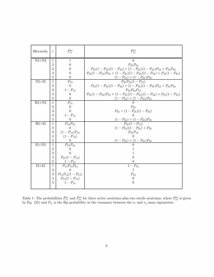
Table 1: The probabilities Pmei and Pm

xi for three active neutrinos plus two sterile neutrinos, where Pmαi is given

by Eq. (25) and Pij is the flip probability at the resonance between the νi and νj mass eigenstates.

6

where Pmαi and P⊕

iβ are respectively the να → νmi transition probability in the supernova and ν⊕

i → νβ transitionprobability in the earth. In the absence of earth matter effects

P⊕ie = |Uei|2 (24)

andPm

αi =∑

j

|Umαj |2Pij , (25)

where Pij is the flip probability between the i and j mass eigenstates, given by Eq. (12). We explicitly give theprobabilities Pm

ei and Pmxi for all the possible mass spectra in Table 1. For further details and the level crossing

diagrams for each of these mass spectra, we refer the reader to [19].

2.2 Effect of the Shock Wave on Pee

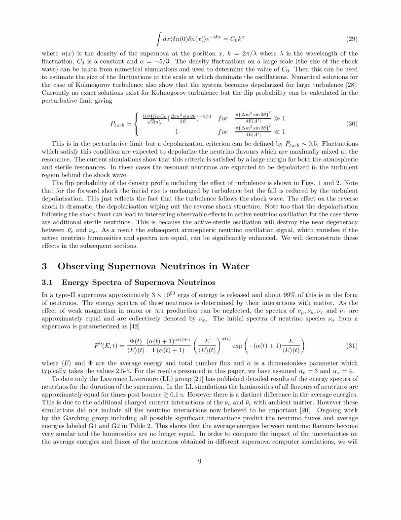
It is believed that when the core of a collapsing supernova reaches nuclear density the collapse rebounds forminga strong outward shock. The shock stalls and is eventually regenerated via neutrino heating. Numericalsimulations show that as well as a forward shock a reverse shock forms and the region behind the shock wave ishighly turbulent [25]. The detailed density profiles from numerical simulations are not available to us, thereforewe consider the simplified profile for the shock wave used in [23, 26]. A schematic diagram showing the densitychange at the shock front for forward shock and for forward and reverse shock is shown by the dashed blacklines in Figs. 1(a) and 2(a).

As can be seen from these figures, the effect of the supernova shock wave is to generate very sharp changesin the density gradient, which is expected to change the flip probability. Since, as mentioned above, the flipprobability is calculated at the position of resonance, the effect of the shock will be to modify the flip probabilityand hence Pee when the shock crosses the resonance density for a certain ∆m2

ji. Also, we see from the figures

that the shock generates fluctuations in the density gradient. This results in the same ∆m2ji producing multiple

resonances which are relatively close together. If we assume that the phase effects can be neglected even in thiscase [39], then the individual resonances can be considered as independent two generation resonances and thenet flip probability PH can be expressed in terms of the multiple flip probabilities Pi as [40, 23]

(

1 − PH PH

PH 1 − PH

)

=∏

i=1,n

(

1 − Pi Pi

Pi 1 − Pi

)

, (26)

where n is the number of resonances occurring for the same ∆m2ji due to the shock effect. In particular, if the

mixing angles are sufficiently large then in the region of the supernova where the density can be approximated asalmost static, the flip probability between the mass eigenstates is approximately zero (the resonance is adiabatic).As the shock wave passes through the resonant density, the flip probability increases to approximately one (theresonance becomes strongly non-adiabatic). As the shock passes over, then in the approximation that there isno turbulence (which will be considered in the next subsection), the flip probability goes back to zero. Theresultant flip probability has a time dependence shown in Figs. 1(b) and 2(b).

Since the resonance densities are different for the different ∆m2ji involved, the shock wave will cross them

at different times. Therefore, one can follow the evolution of the shock wave by following the time profile of thesupernova signal [19]. Also, since the resonance density is determined by the energy of the neutrino, differentenergy neutrinos have their resonance position as different points and thus get affected by the shock at differenttimes. Thus the shock imprints its signature on both the energy spectrum as well as the time profile of theneutrinos arriving on earth. The effect of the shock wave is discussed in [22, 23] for the forward shock andin [25, 26] when there is a reverse shock as well. All these papers used large/megaton water detectors for thesupernova neutrino signal on earth. The possibility of using shock waves to discern the existence of eV masssterile neutrinos in the supernova signal in IceCube was discussed in [19].

2.3 Turbulence

Numerical simulations have shown that a highly turbulent region forms behind the shock wave [41]. Thefluctuations in these turbulence cause flips between the mass eigenstates [27, 28]. The length scale of thefluctuations for which the flips are dominant are at the length scale

7

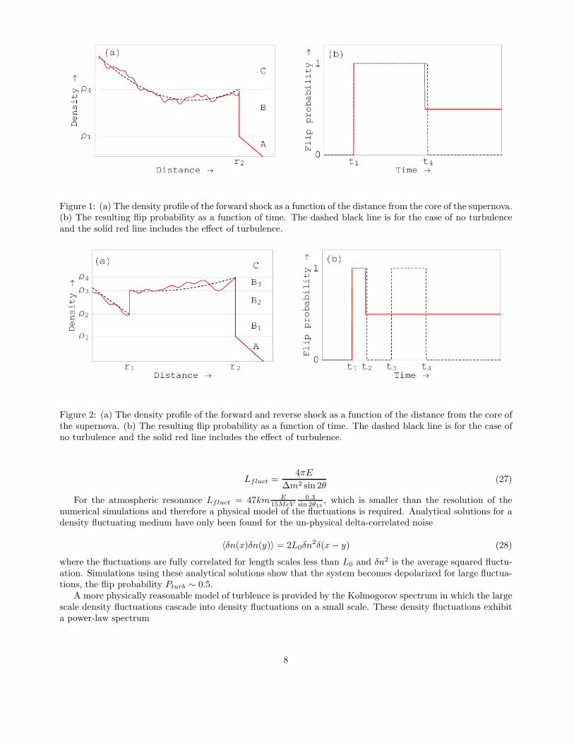
Figure 1: (a) The density profile of the forward shock as a function of the distance from the core of the supernova.(b) The resulting flip probability as a function of time. The dashed black line is for the case of no turbulenceand the solid red line includes the effect of turbulence.

Figure 2: (a) The density profile of the forward and reverse shock as a function of the distance from the core ofthe supernova. (b) The resulting flip probability as a function of time. The dashed black line is for the case ofno turbulence and the solid red line includes the effect of turbulence.

Lfluct =4πE

∆m2 sin 2θ(27)

For the atmospheric resonance Lfluct = 47km E15MeV

0.3sin 2θ13

, which is smaller than the resolution of thenumerical simulations and therefore a physical model of the fluctuations is required. Analytical solutions for adensity fluctuating medium have only been found for the un-physical delta-correlated noise

〈δn(x)δn(y)〉 = 2L0δn2δ(x − y) (28)

where the fluctuations are fully correlated for length scales less than L0 and δn2 is the average squared fluctu-ation. Simulations using these analytical solutions show that the system becomes depolarized for large fluctua-tions, the flip probability Pturb ∼ 0.5.

A more physically reasonable model of turblence is provided by the Kolmogorov spectrum in which the largescale density fluctuations cascade into density fluctuations on a small scale. These density fluctuations exhibita power-law spectrum

8

∫

dx〈δn(0)δn(x)〉e−ikx = C0kα (29)

where n(x) is the density of the supernova at the position x, k = 2π/λ where λ is the wavelength of thefluctuation, C0 is a constant and α = −5/3. The density fluctuations on a large scale (the size of the shockwave) can be taken from numerical simulations and used to determine the value of C0. Then this can be usedto estimate the size of the fluctuations at the scale at which dominate the oscillations. Numerical solutions forthe case of Kolmogorov turbulence also show that the system becomes depolarized for large turbulence [28].Currently no exact solutions exist for Kolmogorov turbulence but the flip probability can be calculated in theperturbative limit giving

Pturb ≃

0.84GF C0√2|n′

0| (∆m2 sin 2θ

2E )−2/3 forπ(∆m2 sin 2θ)2

4E|A′| ≫ 1

1 forπ(∆m2 sin 2θ)2

4E|A′| ≪ 1(30)

This is in the perturbative limit but a depolarization criterion can be defined by Pturb ∼ 0.5. Fluctuationswhich satisfy this condition are expected to depolarize the neutrino flavours which are maximally mixed at theresonance. The current simulations show that this criteria is satisfied by a large margin for both the atmosphericand sterile resonances. In these cases the resonant neutrinos are expected to be depolarized in the turbulentregion behind the shock wave.

The flip probability of the density profile including the effect of turbulence is shown in Figs. 1 and 2. Notethat for the forward shock the initial rise is unchanged by turbulence but the fall is reduced by the turbulentdepolarisation. This just reflects the fact that the turbulence follows the shock wave. The effect on the reverseshock is dramatic, the depolarisation wiping out the reverse shock structure. Note too that the depolarisationfollowing the shock front can lead to interesting observable effects in active neutrino oscillation for the case thereare additional sterile neutrinos. This is because the active-sterile oscillation will destroy the near degeneracybetween νe and νx. As a result the subsequent atmospheric neutrino oscillation signal, which vanishes if theactive neutrino luminosities and spectra are equal, can be significantly enhanced. We will demonstrate theseeffects in the subsequent sections.

3 Observing Supernova Neutrinos in Water

3.1 Energy Spectra of Supernova Neutrinos

In a type-II supernova approximately 3 × 1053 ergs of energy is released and about 99% of this is in the formof neutrinos. The energy spectra of these neutrinos is determined by their interactions with matter. As theeffect of weak magnetism in muon or tau production can be neglected, the spectra of νµ, νµ, ντ and ντ areapproximately equal and are collectively denoted by νx. The initial spectra of neutrino species να from asupernova is parameterized as [42]

F 0(E, t) =Φ(t)

〈E〉(t)(α(t) + 1)α(t)+1

Γ(α(t) + 1)

(

E

〈E〉(t)

)α(t)

exp

(

−(α(t) + 1)E

〈E〉(t)

)

(31)

where 〈E〉 and Φ are the average energy and total number flux and α is a dimensionless parameter whichtypically takes the values 2.5-5. For the results presented in this paper, we have assumed αe = 3 and αx = 4.

To date only the Lawrence Livermore (LL) group [21] has published detailed results of the energy spectra ofneutrinos for the duration of the supernova. In the LL simulations the luminosities of all flavours of neutrinos areapproximately equal for times post bounce & 0.1 s. However there is a distinct difference in the average energies.This is due to the additional charged current interactions of the νe and νe with ambient matter. However thesesimulations did not include all the neutrino interactions now believed to be important [20]. Ongoing workby the Garching group including all possibly significant interactions predict the neutrino fluxes and averageenergies labeled G1 and G2 in Table 2. This shows that the average energies between neutrino flavours becomevery similar and the luminosities are no longer equal. In order to compare the impact of the uncertainties onthe average energies and fluxes of the neutrinos obtained in different supernova computer simulations, we will

9

Model 〈E0νe〉 〈E0

νe〉 〈E0

νx〉 Φ0

νe

Φ0νx

Φ0

νe

Φ0νx

LL 12 15 24 2.0 1.6G1 12 15 18 0.8 0.8G2 12 15 15 0.5 0.5

Table 2: The average energies and total fluxes characterizing the primary neutrino spectra produced insidethe supernova. The numbers obtained in the Lawrence Livermore simulations are denoted as LL, while thoseobtained by the Garching group are denoted as G1 and G2.

present our results using supernova neutrino parameters given by both the Lawrence Livermore and Garchinggroups. Specifically, we consider the three cases shown in Table 2 [25]. For further details, we refer the readerto our earlier paper [19].

3.2 Signal in Water Cerenkov Detectors

Supernova neutrinos with energy in the MeV regime will be dominantly detected in water through the captureof νe on protons4

νe + p → n + e+ . (32)

The emitted positron will be observed in the detector and its energy and time measured. Hence we should beable to get a fairly good reconstruction of the incoming νe energy spectrum and time profile. Neglecting therecoil of the neutron the energy of the neutrino E is related to the energy of the positron through the relationEe = E − 1.29, where all energies are in MeV. The number of events expected in a water Cerenkov detectorfrom a galactic supernova explosion is given by

N =NT

4πD2

∫ ∞

0

∫ ∞

0

F (E) ∗ σ(E) ∗ ε(E) ∗ R(E − 1.29, Ee) dE dEe (33)

where D is the distance of the supernova from earth, NT is the number of target nucleons in 1 megaton of water,E is the energy of the neutrino, Ee is the measured energy of the positron, F(E) is the flux at the detector, asdefined in Eqs. (30) and (37), σ(E) is the cross section, ε(E) is the efficiency of detection and R(E − 1.29, Ee)is the energy resolution function. The efficiency is assumed to be perfect above 7 MeV and vanishing below thisenergy. The energy resolution function for which we assume a Gaussian form

R(ET , Ee) =1√

2πσE

exp

(−(ET − Ee)2

2σ2E

)

, (34)

where ET and Ee are respectively the true and measured energy of the positron and we take the HWHMσE(ET ) =

√E0ET , where E0 = 0.22MeV. This is the same efficiency and energy resolution as used in [25, 43].

Water Cerenkov detectors usually are expected to have time resolution which is of the order of nanosecond. Inwhat follows, we will bin our data either in time bins of 100 ms (at later times) or 10 ms (at earlier times).Since we expect the time resolution of the detector to be at least 3-4 orders of magnitude better, we do notinclude any time resolution function in our calculation of the number of events.

In addition to the total number of events, we also calculate the the average energy of the detected positronsthrough the expression

〈Ee〉 =

∫ ∞0

∫ ∞0

EA ∗ F (E) ∗ σ(E) ∗ ε(E) ∗ R(E − 1.29, EA) dE dEA∫ ∞0

∫ ∞0

F (E) ∗ σ(E) ∗ ε(E) ∗ R(E − 1.29, EA) dE dEA

(35)

4Water Cerenkov detectors have other detection channels whereby they can observe νe and νx (electron scattering and chargedand neutral current interactions on 16O). However, the cross-section for these processes are much smaller and hence they are notconsidered here.

10

We show both the number of events as well as the average energy as a function of time. We also showthe statistical uncertainties expected in 1 megaton water Cerenkov detectors. The statistical error in the totalnumber of events are estimated as

σN =√

N , (36)

while that in the average energy is calculated as

σ〈E〉 =

√

〈E2e 〉 − 〈Ee〉2

N, (37)

where σ〈E〉 is the error in the average energy, N is the number of events, 〈E〉 is the average energy and 〈E2〉 isthe average energy squared.

The neutrino flux in the detector isFβ =

∑

α

F 0αPαβ (38)

where Pαβ is the oscillation probability and is given in Eqs. (23)-(25) and F 0α is the initial flux of να given in

Eqn. (31).

3.3 Input Supernova and Oscillation Parameters

In what follows, we will present results for the typical values for the fluxes and average energies given in Table2 for the LL, G1 and G2 “models”. For the neutrino oscillation parameters, we assume the best-fit values∆m2

21 = 8 × 10−5 eV2, sin2 θ12 = 0.31 and ∆m231 = 2.5 × 10−3 [10]. For θ13, we assume that it is large enough

so that away from the shock, the ∆m231 driven resonant transition is fully adiabatic. Typically, this would be

satisfied for sin2 θ13 ∼> 10−3.The other oscillation parameters relevant for supernova neutrino oscillations in the 3+2 scenario are con-

strained by the combined data from Bugey, CHOOZ, CCFR84, CDHS, KARMEN, NOMAD, and LSND [29, 44].If we restrict the mass squared differences to lie in the sub-eV regime then the best-fit comes at ∆m2

41 = 0.46eV2, ∆m2

51 = 0.89 eV2, Ue4 = 0.09, Ue5 = 0.125, Uµ4 = 0.226 and Uµ5 = 0.16 [31]. These values of theoscillation parameters give fully adiabatic transition at the resonance in the supernova when the shock is notpresent.

3.3.1 Sterile neutrino sensitivity

In the detailed estimates presented below we use the sterile neutrino parameters consistent with an explanationof the LSND experiment. However it is important to stress that the sensitivity to sterile neutrinos is muchbetter than is needed to probe the LSND range and that, even if MiniBoone should rule out the sterile mixingangle regime used in our estimates, supernovae neutrino signals will still be important in the search for evidencefor sterile neutrinos. It is straightforward to quantify the range of sensitivity. To observe the time dependenteffects in the signal due to sterile neutrinos, the adiabaticity of the sterile resonances needs to be changed bythe shock wave and/or the turbulence. For mixing angles sin2 θij . 4 × 10−6 the sterile resonances would benon-adiabatic for the entire time of interest. As a result there would be no oscillations into sterile neutrinosand the signal would be equivalent to that of only 3 active neutrinos. For sin2 θij & 4 × 10−4 the resonancewould be adiabatic in the regions behind (with no turbulence) and in front of the shock wave. In this range theactive-sterile resonant mixig effects are measureable. The situation is summarised in Table 3.

For 4× 10−6 < sin2 θij < 4× 10−4 there is a “transition region”, in which the effects discussed in this papercould be observed but may be less prominent. To quantify this first note that within this region of parameterspace the mixing angles are sufficiently large such that each resonance is adiabatic in the absence of the shockwave. As well as changing the adiabaticity of each resonance the mixing angles change the relative proportionof each flavour eigenstate in each mass eigenstate, as a result changing the νe flux, Fe in the detector. Theapproximate Fe for small sterile mixing angles is shown in Table 4. If the sterile mixing angles and θ13 arescaled as θij → kθij , where i=1,2, and j=3-5, and k < 1, Fe is approximately unchanged except for the N2+I3and H2+N3 mass hierarchies. If the flux is unchanged both the number of events and the average energies are

11

sin2 θij Region

6 × 10−3 . sin2 θij Sensitivity range of MiniBoone4 × 10−4 . sin2 θij Maximal effect of shock

4 × 10−6 . sin2 θij . 4 × 10−4 Transition regionsin2 θij . 4 × 10−6 No effect of shock

Table 3: The effect of the shock wave for the parameter space of sin2 θij with i=1,2 and j=3-5.

unchanged. For the cases of N2+I3 and H2+N3 mass hierarchies Fnoshock is scaled as Fnoshock → k2Fnoshock. Asa result the flux and therefore number of observed events before and after the propagation of a shock wave scaleas k2, the statistical uncertainties scale as k−1 and the average energies remain unchanged. Therefore for k < 1the number of events decreases, and the uncertainties in the number of events and average energies increases.As the shock wave passes through the resonance the flux is Fe ≃ Fshock, which is independent of k. Thereforethe total number of events is approximately unchanged. However, as the shock passes through a resonance thenumber of events increases, these corresponds to the lowest energy neutrinos, as a result the average energydecreases. For smaller k the relative increase in the number of events is larger and therefore the decrease in theaverage energy is larger. At later times there is an increase in the average energy as the resonance condition issatisfied for higher energy neutrinos, for smaller k the relative increase is larger and therefore the increase in theaverage energy is larger. As a result the structure of the average energy plot remains but is stretched for smallerk. Simulations show that the number of events during the shock propagation is approximately independent ofk for k . 1 and the average energy plot is stretched as described above.

3.4 Three active neutrinos

We first consider the case of a “standard” supernova at 10 kpc from earth. If the mass hierarchy of the neutrinosis inverted, the flux of anti-electron neutrinos in the detector is given by

Fe = F 0x + Pee(F

0e − F 0

x ) (39)

where Pee is given by Eq. (15). For the values of sin2 θ13 ∼> 10−3 that we assume throughout this paper, P13 ≃ 0in the absence of shock and the flux of νe at the detector Fe ≃ F 0

x . As the shock crosses the resonance density,P13 ≃ 1 as discussed in section 2.2 and the flux of νe at the detector is given by Fe ≃ (1− |Ue1|2)F 0

x + |Ue1|2F 0e .

If the average energy of νx is larger than that of νe as obtained in the LL simulations, the average energy willdecrease as a result of the shock effect. This can be seen from Fig. 3(a), where we show the time evolution of theaverage energy of the neutrinos detected in a megaton water Cerenkov detector. The band shows the statisticalerror expected in the measured average energy. For no shock (NS) the average energy remains almost constantwith time. On the other hand the average energy decreases and hence shows “bumps” in the time profile as theshock crosses the position of the ∆m2

31 driven resonance. We get a single bump for the forward shock only anddouble bump when the reverse shock is also present. This is due to the shape of the flip probability shown inFigs. 1 and 2. Also shown (in Fig. 3(c) and Fig. 3(e)) is what is expected if the difference between the averageenergies of the νe and νx created in the supernova were not so well separated. We notice that even though theeffect of the shock is less dramatic, nonetheless it is still there and should be observable. Particularly note thatfor G2 the average energy of νe and νx are equal, therefore the change in the average energy measured by thedetector is due to the change in the number of detected neutrinos. In Fig. 4 we show the total number of eventsexpected for the LL (panel (a)), G1 (panel (c)) and G2 (panel (e)) cases, with and without the shock effects.Since the cross section for the detection cross section increases quadratically with energy, the number of eventswill decrease when the shock crosses the ∆m2

31 resonance density and this results in lowering of the number ofevents and hence again gives single bump and double bump for the forward and forward+reverse shock casesrespectively, as a function of time.

The corresponding results taking into account the effects of turbulence are shown in right-hand panels ofFigs. 3 and 4. Panels (b), (d) and (f) in these figures correspond to the LL, G1 and G2 simulations respectively.The inclusion of turbulence changes the signal for t & 5s. This is when the resonant density is in the turbulentregion. As discussed before, the system is largely depolarized giving P13 ≃ 1/2. The flux at the detector when

12

Hierarchy Fnoshock Fshock

N2+N3 |Ue1|2F 0e P24P25|Ue2|2F 0

x

N2+I3 |Ue3|2F 0e + (|Ue4|2 + |Ue5|2)F 0

x |Ue1|2P13F0e + ((P24 + P25)|Ue2|2

+P24P25(|Ue1|2 − |Ue2|2))F 0x

H2+N3 |Ue4|2F 0e + (|Ue3|2 + |Ue5|2)F 0

x P24|Ue1|2F 0e + P25|Ue2|2F 0

x

H2+I3 |Ue2|2F 0x P25|Ue1|2F 0

x

I2+N3 |Ue2|2F 0x P24P25|Ue1|2F 0

e

I2+I3 (|Ue1|2 + |Ue2|2)F 0x −P13|Ue1|2F 0

x

Table 4: The flux of neutrinos in the approximation that |Ue1|2, |Ue2|2 >> |Ue3|2, |Ue4|2, |Ue5|2 and P1i, P3i ≃P2i, where i=4 or 5. The total flux in presence of shock is given by Fe = Fnoshock +Fshock, where Fnoshock = Fe

without the shock and Fshock is the extra component due to the shock effect.

the shock crosses the resonance region is now given by Fe ≃ (1 − 0.5|Ue1|2)F 0x + 0.5|Ue1|2F 0

e . For the samearguments as before, the average energy is lower than the case of no shock, however the effect now is much lessthan the case where turbulence was not considered. Therefore, the single and double bump features expectedfrom shock effects get smeared out to a large extent. However, we still see a non-trivial variation of the expectedaverage energy in the detector as a function of time, both for the LL and G1/G2 simulations.

3.5 Three active and two sterile neutrinos

For the case where we have two extra light sterile neutrinos in addition to the three active ones, the situationgets a lot more involved due to the possibility of multiple resonances as discussed in section 2.1. The effect ofthe shock is also richer here since the shock passes through the different resonance densities at different times.In Table 4 the resultant neutrino flux at the detector is given in terms of the original neutrino fluxes produced,for the different neutrino mass spectra considered, for both with and without shock effects. We reiterate thatwe have chosen mixing angles such that in absence of shock effects all resonances are adiabatic. The effect ofthe shock is to turn the adiabatic resonant transition into non-adiabatic ones, as discussed before. For the casewhere sterile neutrinos are present, the change in number of events are characterized by the oscillations of activeneutrinos into sterile species and vice-versa. Thus in this case, difference in the initial neutrino energy spectra isnot a pre-requisite for observing resonant oscillations and shock effects, unlike in the case of 3 active neutrinosonly. As the shock moves in time, its effect is imprinted on the time dependence of the neutrino signal, as inthe case of 3 active neutrinos only. However, with sterile neutrinos there are further modulations in the signalbecause the shock passes through the additional sterile resonances. The number of resonances is dependent onthe number of sterile neutrinos as well as the neutrino mass spectrum and therefore the expected signal is oftendifferent for each scenario, as described in detail in [19]. In fact, as we will see, even when the shock passesthrough the ∆m2

31 driven active resonance, the time profile and energy spectrum of the observed neutrinos inmany of the possible mass spectrum listed in Eqs. (17)-(22), are different than what is expected for the case of3 active neutrinos only. Typically, the shock crosses the multiple “sterile resonances” at very early times (t ∼< 2sec), while it crosses the ∆m2

31 driven “active resonance” at later times (t ∼> 3 sec). Therefore in what follows,we will present results separately at late and early times to show clearly the effect of the shock wave on theneutrino signal in the detector. For later times, we will consider time bins of 100 ms, while at earlier times sincethe time dependence is much more sharp, we present our results for smaller time bins of 10 ms.

3.6 Neutrino signal at late times

We begin by discussing the evolution of the expected neutrino event rate and average energy at later times. Thetotal number of events for the different mass spectra are shown in Fig. 5 while the expected average energies

13

are shown in Fig. 6, at times between t = 3 − 12s. These plots show the impact on the signal when the shockwave passes through the ∆m2

31 resonance between active neutrinos. In panels (a)-(d) of Figs. 5 and 6 we showonly the mass spectrum cases where ∆m2

31 < 0, in which we have resonance and hence also shock effects. Whichmass spectra will get the shock effects can be easily seen from Table 4. Since at late times the resonance thatgets affected by the shock is the ∆m2

31 driven resonance between the 1-3 states, the relevant jump probabilityinvolved is P13. All other jump probabilities are zero here, from our choice of the mixing angles. We can seefrom Table 4 that the N2+I3 and I2+I3 are the only cases which will get affected. For all the other mass spectrapossible, we do not expect any modulation in the signal at late times due to shock effects. Hence we show onlythe signal for the N2+I3 and I2+I3 cases. For comparison we show in the last 2 panels of these figures the caseof only active neutrinos (I3).

In the approximation that |Ue3|2, |Ue4|2 and |Ue5|2 can be neglected in comparison to |Ue1|2 and |Ue2|2, wenote from Table 4 that in absence of shock,

I3 ⇒ Fe ≃ F 0x , (40)

N2 + I3 ⇒ Fe ≃ 0 , (41)

I2 + I3 ⇒ Fe ≃ F 0x , (42)

whereas when the shock passes through the 1-3 resonance the fluxes are modified to,

I3 ⇒ Fe ≃ F 0x (1 − P13|Ue1|2) + P13|Ue1|2F 0

e , (43)

N2 + I3 ⇒ Fe ≃ |Ue1|2P13F0e , (44)

I2 + I3 ⇒ Fe ≃ (1 − P13|Ue1|2)F 0x . (45)

By comparing Eqs. (40)-(42) we note that in absence of shock, while the fluxes are same for I3 and I2+I3spectra, N2+I3 predicts almost zero fluxes. The black bands in Fig. 5 corroborate the above statement. Whenthe shock passes through the ∆m2

31 resonance it increases the νe flux for N2+I3, while it decreases the same forI2+I3, as can be seen by comparing Eqs. (41) and (42) with Eqs. (44) and (45). In the case of I3, the resultantflux is an admixture of a fraction of the initial νe and νx fluxes. However, since the average energy of initial νe

flux was smaller, the total number of events goes down in the detector when the shock passes through the 1-3resonance even in this case. We stress that the sterile cases are qualitatively different from the I3 case, since forthem the net number flux sees a big increase or decrease due to shock. Therefore, while for I3, the effect of theshock wave comes predominantly through the difference in the average energy of νe and νx, for sterile cases wesee a combined effect coming from a direct change in the number of neutrinos arriving on earth as well as thedifference in the energy spectra of the different species.

For all the mass spectra shown, under the assumption that there is no turbulence, typically a single bumpis observed for a forward shock and a double bump for a forward and reverse shock, as expected from the shapeof the flip probability shown in Figs. 1 and 2. The effect of taking the turbulence into account is to smear thesesharp changes in the oscillation probability due to the effective depolarizing of the resonances. With turbulence,a single bump is observed, followed by a region in which the number of events are typically different from whatis expected for no turbulence. This can be seen in the right-hand panels in Fig. 5.

The expected average energies for the N2+I3 and I2+I3 cases also show a very striking evolution with timeat t ∼> 3s, which is very different from that predicted by I3. In the case of I3, the average energy decreases inpresence of shock as expected, since the shock reduces the conversion probability of the high energy νx into νe,thereby decreasing the average energy. Thus it usually shows 1 sharp decrease for forward shock and 2 sharpfalls for forward+reverse shock. On the other hand both N2+I3 and I2+I3 predict that the average energyfluctuates on both sides of the average energy expected in absence of shock. The key issue to note here is thatthe position of resonance is determined by the energy of the neutrino. The higher (lower) energy neutrinos gothrough the resonance at lower (higher) density. Since the shock moves from higher to lower densities in time,the lower energy neutrinos are affected by the shock earlier than the higher energy ones. For the sterile cases,the effect is more subtle. Here the time evolution of the average energy is a combined effect of the change inthe total flux as well as the energy dependence of the resonance position. For the I2+I3 case since resonancehappens for lowest energy neutrinos first, the effect of the shock is to reduce them in the flux (cf. Eq.(42) and(45)), thereby increasing the average energy. Eventually, the shock goes through higher energy resonances, and

14

this then reduces the average energy. For the N2+I3 case also the resonance happens for the lowest energyneutrinos first, but now the shock effect increases them in the flux and thereby decreases the average energy.Eventually, the shock goes through the high energy resonances, increasing the average energy.

The right-hand panels of Fig. 6 show the average energy after turbulence is taken into consideration. Thepresence of turbulence has a typical effect on the time evolution of both the total number of events and theaverage energy deposited by the (anti)neutrinos. One can see that without turbulence both the average energyand number of events after the passage of (both) shock(s) go back to its pre-shock value. This is because thePee before and after the shock are exactly the same in this case. However, since the turbulence changes theflip probability permanently to Pij behind the shock, the number of events and average energy are consistentlylower once the shock crosses the resonance point.

3.7 Neutrino signal at early times

In Figs. 7 and 9 we show the number of predicted events and average energies as a function of time (in absenceof turbulence) for the 5 different mass spectra, between t = 0.1− 1.5s, in short time bins of 10 ms. Figs. 8 and10 show the corresponding results when turbulence is taken into account. We do not show results for the I2+I3spectra here since, as can be seen from Table 4, it depends only on P13 which will have shock effects only atthe ∆m2

31 resonance at late times.As in the previous subsection, Fig. 7 can be understood in terms of the flux predictions in the presence and

absence of the shock, given in Table 4. The only difference is that at early times the shock passes through thesterile resonances and hence we expect contributions coming from the jump probabilities associated with thesterile resonances. In particular, we note that in the absence of shock, the predicted flux on earth is almostzero for N2+I3 and H2+N3, while for H2+I3 and I2+N3 we expect the flux to be |Ue2|2F 0

x and for N2+N3 itis predicted to be |Ue1|2F 0

x . Since |Ue1|2 > |Ue2|2, the expected signal is larger for N2+N3. These features areevident from Fig. 7. As a result of the shock we see a modulation in the resultant signal visible as bumps in thefigure. Note that in all the 5 cases shown, the shock effect increases the number of events. The shock poweredmodulations get affected when turbulence is taken into account and the corresponding results are shown in Fig.8.

Fig. 9 shows how the average energy evolves at early times. As we had seen at later times, the effect of theshock wave is to make the average energy fluctuate on both sides of the corresponding static density case. Thereason for the initial average energy decrease and subsequent increase is also the same as that discussed in theprevious subsection. Fig. 10 shows the average energy evolution when the effect of turbulence is considered. Therapid fluctuations are mellowed due to the presence of turbulence, however we still see statistically significantfluctuations in the average energy at very early times, a feature which, if observed, would provide an almostmodel independent signal of the presence of extra sterile neutrino species which are mixed mildly with the activeneutrinos.

As the water Cerenkov detector can measure the energy of the incoming neutrino rather efficiently, the eventscan be binned in energy as well as time. In Fig. 11 we present the number of events expected in energy binsof width 10 MeV and time bins of 10 ms. We show results for the N2+I3 spectrum only as an example. Thisfigure is shown for only early times to illustrate the effect of the sterile resonances. As the resonance densitiesare energy dependent, the propagation of the shock wave can be observed when the events are binned in energyand time. The shock wave crosses the resonant density corresponding to neutrinos with lower energies first,therefore the characteristic ’bumps’ are observed in the lower energy bins first. The presence of such energyand time dependent bumps in the resultant signal in the detector provides a ’smoking gun’ signal for sterileneutrinos.

4 Comparison and Discussions

In Table 5 we show the model independent characteristic features in the expected signal for the eight differentcases considered in this paper, the two only active cases (N3 and I3) and the six active plus sterile cases. Thetime interval is divided into early (t ∼< 2 s) and late (t ∼> 3 s) times, as before. For each case we state if weexpect large (L) or very small (S) number of events in the 2 time zones. We also indicate in the table whether

15

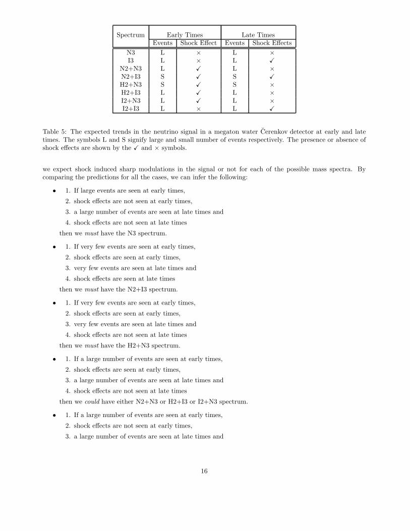
Spectrum Early Times Late TimesEvents Shock Effect Events Shock Effects

N3 L × L ×I3 L × L X

N2+N3 L X L ×N2+I3 S X S XH2+N3 S X S ×H2+I3 L X L ×I2+N3 L X L ×I2+I3 L × L X

Table 5: The expected trends in the neutrino signal in a megaton water Cerenkov detector at early and latetimes. The symbols L and S signify large and small number of events respectively. The presence or absence ofshock effects are shown by the X and × symbols.

we expect shock induced sharp modulations in the signal or not for each of the possible mass spectra. Bycomparing the predictions for all the cases, we can infer the following:

• 1. If large events are seen at early times,

2. shock effects are not seen at early times,

3. a large number of events are seen at late times and

4. shock effects are not seen at late times

then we must have the N3 spectrum.

• 1. If very few events are seen at early times,

2. shock effects are seen at early times,

3. very few events are seen at late times and

4. shock effects are seen at late times

then we must have the N2+I3 spectrum.

• 1. If very few events are seen at early times,

2. shock effects are seen at early times,

3. very few events are seen at late times and

4. shock effects are not seen at late times

then we must have the H2+N3 spectrum.

• 1. If a large number of events are seen at early times,

2. shock effects are seen at early times,

3. a large number of events are seen at late times and

4. shock effects are not seen at late times

then we could have either N2+N3 or H2+I3 or I2+N3 spectrum.

• 1. If a large number of events are seen at early times,

2. shock effects are not seen at early times,

3. a large number of events are seen at late times and

16

4. shock effects are seen at late times

then we could have either I3 or I2+I3 spectrum. This degeneracy can be split by measurng the energydependence (c.f. Figure 6 (c) and (d)).

Therefore, from the Table 5 we conclude that, irrespective of model uncertainties, the presence of sterileneutrinos can be easily proved from modulation of the signal due to shock effects at early time. Only the I2+I3case does not give any time modulation, even though the sterile neutrinos are present in this case. In addition,from the point-wise discussion above we can see how well we can distinguish one mass spectrum from the other.N3, N2+I3 and H2+N3 can be uniquely determined by comparing early time behavior of the signal with itslate time behavior. The N2+N3, H2+I3 and I2+N3 can be separated from the rest, but since they predictsimilar trends at early and late times, one will be need a more careful model dependent study to unambiguouslydisentangle them from each other. Similarly, though I3 and I2+I3 can be separated from the other spectra, onewill need a more careful analysis to distinguish between the two.

5 Summary and Conclusions

Model independent information about the neutrino mass spectrum can be obtained through observation ofsignatures of supernova shock wave(s) on the resultant neutrino signal in terrestrial detectors. In particular,such signals probe the existence of extra sterile neutrino through their possible resonant transition with activeneutrinos inside the supernova. Oscillations between sterile neutrino and active ones are characterized by uniquesignatures in the final neutrino energy spectrum as well as their evolution with time. While the impact of thepresence of sterile neutrinos on the time evolution of the neutrino is due to shock effects, their impact on theresultant neutrino flux and spectra comes from neutrino oscillations both with and without shock effects.

Concerns had been raised recently over the observability of the shock effects due to the turbulent densityvariations following the shock wave which prove to be very important. In this paper we made a detailed studyof the turbulent shock effects on the neutrino induced galactic supernova signal expected in megaton waterCerenkov detector. Water detectors can give information on the number, the energy spectrum, as well the timeprofile of the arriving (anti)neutrinos. We have shown that the impact of the supernova shock waves is evidentin the neutrino signature in megaton water Cerenkov detectors in all of these, making this class of detectorsextremely good for studying shock effects. We have considered the impact of the turbulence left behind by theshock wave and have seen that although the shock effect is diluted, it is still significant and we still expect toobserve them in the megaton class of detectors. We have concentrated on the discernable signatures of sterileneutrinos, which might be mixed mildly with the 3 active neutrinos. We have illustrated the effects using sterileneutrino parameters which were chosen in a fit to all neutrino data including LSND. However we showed that theobservable signals persist for much smaller mixing angles than are observable by the LSND (or MiniBOONE)experiments. Hence our results are relevant whatever the outcome of the MiniBOONE data.

The most striking evidence for sterile neutrinos in the supernova neutrino signal are sharp bumps at t ∼< 1secinthe observed number flux as well as the average energy of the νe detected through their capture on protons inmegaton water detectors. These can be caused only by sterile neutrino resonances inside the supernova. Onlythe I2+I3 case for the mass spectrum does not predict these early time shock induced modulations in the signal.In addition, a model independent comparison of the signal trend between early and late times can give us arather unambiguous signature on 3 of the 8 possible mass spectra considered in this paper. The N3, N2+I3and H2+N3 cases predict unique combination of behavior at early and late times and hence can be determinedmodel independently from the observations. The remaining 5 cases can be classed into 2 categories dependingon their combination of predicted trends at early and late times. Distinguishing the I3 from the I2+I3 spectrawould require a more careful model dependent analysis of the future supernova neutrino data. Similarly, theN2+N3, H2+I3 and I2+N3 can be separated from the relative differences in their predictions of average energyand number of events as a function of time.

One important byproduct of the turbulent effects involving active-sterile neutrino mixing is that, even if theenergy spectrum and luminosisites of the active neutrinos are initially the same, the depolarising effect of theturbulence for the active sterile resonances in the wake of the shock front will make the active neutrino spectraspectra and luminosities significantly different. As a result the atmospheric neutrino resonant effects involving

17

the active neutrinos in the presence of sterile neutrinos may be expected to give rise to more significant effectsin the supernova neutrino signal than is the case without sterile neutrinos.

Acknowledgment

We thank T. Kajita for discussion on water Cerenkov detectors. SC wishes to thank PPARC and the Universityof Oxford for financial support during this work.

References

[1] R. M. Bionta et al., Phys. Rev. Lett. 58 (1987) 1494.

[2] K. Hirata et al. [KAMIOKANDE-II Collaboration], Phys. Rev. Lett. 58 (1987) 1490.

[3] H. A. Bethe, Astrophys. J. 412, 192 (1993). V. Barger, D. Marfatia and B. P. Wood, Phys. Lett. B 532, 19(2002); H. Minakata and H. Nunokawa, Phys. Lett. B 504, 301 (2001); C. Lunardini and A. Y. Smirnov,Astropart. Phys. 21, 703 (2004); A. Mirizzi and G. G. Raffelt, Phys. Rev. D 72, 063001 (2005).

[4] B. T. Cleveland et al., Astrophys. J. 496, 505 (1998); J. N. Abdurashitov et al. [SAGE Collaboration],J. Exp. Theor. Phys. 95, 181 (2002); [Zh. Eksp. Teor. Fiz. 122, 211 (2002)] W. Hampel et al. [GALLEXCollaboration], Phys. Lett. B 447, 127 (1999); C. Cattadori, Talk at Neutrino 2004, Paris, France, June 14-19, 2004; S. Fukuda et al. [Super-Kamiokande Collaboration], Phys. Lett. B 539, 179 (2002); B. Aharmimet al. [SNO Collaboration], Phys. Rev. C 72, 055502 (2005).

[5] T. Araki et al. [KamLAND Collaboration], Phys. Rev. Lett. 94, 081801 (2005).

[6] M. Apollonio et al., Eur. Phys. J. C 27, 331 (2003); F. Boehm et al., Phys. Rev. D 64, 112001 (2001).

[7] Y. Ashie et al. [Super-Kamiokande Collaboration], Phys. Rev. D 71, 112005 (2005).

[8] E. Aliu et al. [K2K Collaboration], Phys. Rev. Lett. 94, 081802 (2005).

[9] D. G. Michael et al. [MINOS Collaboration], Phys. Rev. Lett. 97, 191801 (2006).

[10] M. Maltoni et al., New J. Phys. 6, 122 (2004), hep-ph/0405172 v5; S. Choubey, arXiv:hep-ph/0509217;S. Goswami, Int. J. Mod. Phys. A 21, 1901 (2006); A. Bandyopadhyay et al., Phys. Lett. B 608, 115(2005); G. L. Fogli et al., Prog. Part. Nucl. Phys. 57, 742 (2006).

[11] K. Anderson et al., arXiv:hep-ex/0402041.

[12] Y. Itow et al., arXiv:hep-ex/0106019.

[13] D. S. Ayres et al. [NOvA Collaboration], arXiv:hep-ex/0503053.

[14] C. Volpe, J. Phys. G 34, R1 (2007); S. K. Agarwalla, S. Choubey and A. Raychaudhuri,arXiv:hep-ph/0610333 and references therein.

[15] C. Albright et al. [Neutrino Factory/Muon Collider Collaboration], arXiv:physics/0411123.

[16] A. S. Dighe and A. Y. Smirnov, Phys. Rev. D 62, 033007 (2000); C. Lunardini and A. Y. Smirnov,JCAP 0306, 009 (2003); C. Lunardini and A. Y. Smirnov, Nucl. Phys. B 616, 307 (2001); S. Choubey,D. Majumdar and K. Kar, J. Phys. G 25, 1001 (1999); G. Dutta et al., Phys. Rev. D 61, 013009 (2000);A. S. Dighe et al., JCAP 0401, 004 (2004); H. Minakata et al., Phys. Lett. B 542, 239 (2002).

[17] A. S. Dighe, M. T. Keil and G. G. Raffelt, JCAP 0306, 006 (2003); A. Bandyopadhyay, S. Choubey,S. Goswami and K. Kar, arXiv:hep-ph/0312315; T. Marrodan Undagoitia, F. von Feilitzsch, M. Goger-Neff, K. A. Hochmuth, L. Oberauer, W. Potzel and M. Wurm, J. Phys. Conf. Ser. 39, 287 (2006);S. Skadhauge and R. Z. Funchal, arXiv:hep-ph/0611194.

18

[18] A. S. Dighe, M. T. Keil and G. G. Raffelt, JCAP 0306, 005 (2003).

[19] S. Choubey, N. P. Harries, and G. G. Ross Phys. Rev. D 74, 053010 (2006).

[20] S. Hannestad and G. Raffelt, Astrophys. J. 507, 339 (1998); R. Buras et al., Astrophys. J. 587, 320(2003); M. T. Keil, G. G. Raffelt and H. T. Janka, Astrophys. J. 590, 971 (2003); M. Liebendoerfer et

al., Astrophys. J. 620, 840 (2005). G. G. Raffelt, M. T. Keil, R. Buras, H. T. Janka and M. Rampp,arXiv:astro-ph/0303226.

[21] K. Takahashi, M. Watanabe, K. Sato and T. Totani, Phys. Rev. D 64, 093004 (2001).

[22] R. C. Stimesrato, G. M. Fuller, arXiv:astro-ph/0205390.

[23] G. L. Fogli, E. Lisi, A. Mirizzi and D. Montanino, Phys. Rev. D 68, 033005 (2003).

[24] V. Barger, P. Huber and D. Marfatia, Phys. Lett. B 617, 167 (2005).

[25] R. Tomas, M. Kachelriess, G. Raffelt, A. Dighe, H. T. Janka and L. Scheck, JCAP 0409, 015 (2004).

[26] G. L. Fogli, E. Lisi, A. Mirizzi and D. Montanino, JCAP 0504, 002 (2005).

[27] G. L. Fogli, E. Lisi, A. Mirizzi and D. Montanino, arXiv:hep-ph/0603033.

[28] A. Friedland, and A. Gruizinov arXiv:astro-ph/0607244.

[29] C. Athanassopoulos et al., (The LSND Collaboration) Phys. Rev. Lett. 77, 3082 (1996); C. Athanas-sopoulos et al., (The LSND Collaboration) Phys. Rev. Lett. 81, 1774 (1998).

[30] J. J. Gomez-Cadenas and M. C. Gonzalez-Garcia, Z. Phys. C 71, 443 (1996); S. Goswami, Phys. Rev. D55, 2931 (1997). S. M. Bilenky, C. Giunti and W. Grimus, Eur. Phys. J. C 1, 247 (1998).

[31] M. Sorel, J. M. Conrad and M. H. Shaevitz, Phys. Rev. D 70, 073004 (2004).

[32] A.Strumia, “Neutrino masses and mixings and...”, http://astrumia.web.cern.ch/astrumia/review.pdf

[33] http://www-boone.fnal.gov/

[34] L. Wolfenstein, Phys. Rev. D 17, 2369 (1978);

[35] S. P. Mikheev and A. Y. Smirnov, Sov. J. Nucl. Phys. 42, 913 (1985) [Yad. Fiz. 42, 1441 (1985)];S. P. Mikheev and A. Y. Smirnov, Nuovo Cim. C 9, 17 (1986).

[36] V. D. Barger, K. Whisnant, S. Pakvasa and R. J. N. Phillips, Phys. Rev. D 22, 2718 (1980).

[37] E. Lisi, A. Marrone, D. Montanino, A. Palazzo and S. T. Petcov, Phys. Rev. D 63, 093002 (2001);G. L. Fogli, E. Lisi, D. Montanino and A. Palazzo, Phys. Rev. D 65, 073008 (2002); A. Friedland, Phys.Rev. D 64, 013008 (2001).

[38] S. T. Petcov, Phys. Lett. B 200, 373 (1988).

[39] B. Dasgupta and A. Dighe, arXiv:hep-ph/0510219.

[40] T. K. Kuo and J. Pantaleone, Rev. Mod. Phys. 61, 937 (1989); T. K. Kuo and J. Pantaleone, Phys. Rev.D 37, 298 (1988).

[41] K. Kifonidis, T. Plewa, L. Scheck, H. T. Janka, and E. Muller arXiv:astro-ph/0511369.

[42] M. T. Keil, arXiv:astro-ph/0308228; M. T. Keil, G. G. Raffelt and H. T. Janka, Astrophys. J. 590, 971(2003).

[43] R. Tomas, D. Semikoz, G. G. Raffelt, M. Kachelriess and A. S. Dighe, Phys. Rev. D 68 (2003) 093013

[44] Y. Declais et al., Phys. Lett. B 338, 383 (1994); F. Dydak et al., Phys. Lett. B 134, 281 (1984); I. E. Stock-dale et al., Phys. Rev. Lett. 52, 1384 (1984); B. Armbruster et al. [KARMEN Collaboration], Phys. Rev.D 65, 112001 (2002); P. Astier et al. [NOMAD Collaboration], Phys. Lett. B 570, 19 (2003).

19

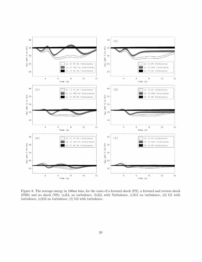
Figure 3: The average energy in 100ms bins, for the cases of a forward shock (FS), a forward and reverse shock(FRS) and no shock (NS): (a)LL no turbulence, (b)LL with Turbulence, (c)G1 no turbulence, (d) G1 withturbulence, (e)G2 no turbulence, (f) G2 with turbulence.

20

Figure 4: The number of events in 100ms bins, for the cases of a forward shock (FS), a forward and reverseshock (FRS) and no shock (NS): (a)LL no turbulence, (b)LL with Turbulence, (c)G1 no turbulence, (d) G1with turbulence, (e)G2 no turbulence, (f) G2 with turbulence.

21

Figure 5: The number of events in 100ms bins, for the cases of a forward shock (FS), a forward and reverse shock(FRS) and no shock (NS): (a)N2 + I3 no turbulence, (b)N2 + I3 with turbulence, (c)I2 + I3 no turbulence,(d)I2 + I3 with turbulence, (e)I3 no turbulence, (f)I3 with turbulence.

22

Figure 6: The average energy in 100 ms bins, for the cases of a forward shock (FS), a forward and reverse shock(FRS) and no shock (NS), with the initial energy spectra G1 as discussed in the text: (a)N2 + I3 no turbulence,(b)N2 + I3 with turbulence, (c)I2 + I3 no turbulence, (d)I2 + I3 with turbulence, (e)I3 no turbulence, (f)I3with turbulence.

23

Figure 7: The number of events in 10 ms bins, for the cases of ∆m241 = 0.46MeV 2 and ∆m2

51 = 0.54MeV 2,with no turbulence, a forward shock (FS), a forward and reverse shock (FRS) and no shock (NS), with theinitial energy spectra G1 as discussed in the text:(a)N2 + N3, (b)N2 + I3, (c)H2 + N3, (d)H2 + I3, (e)I2 +N3.

24

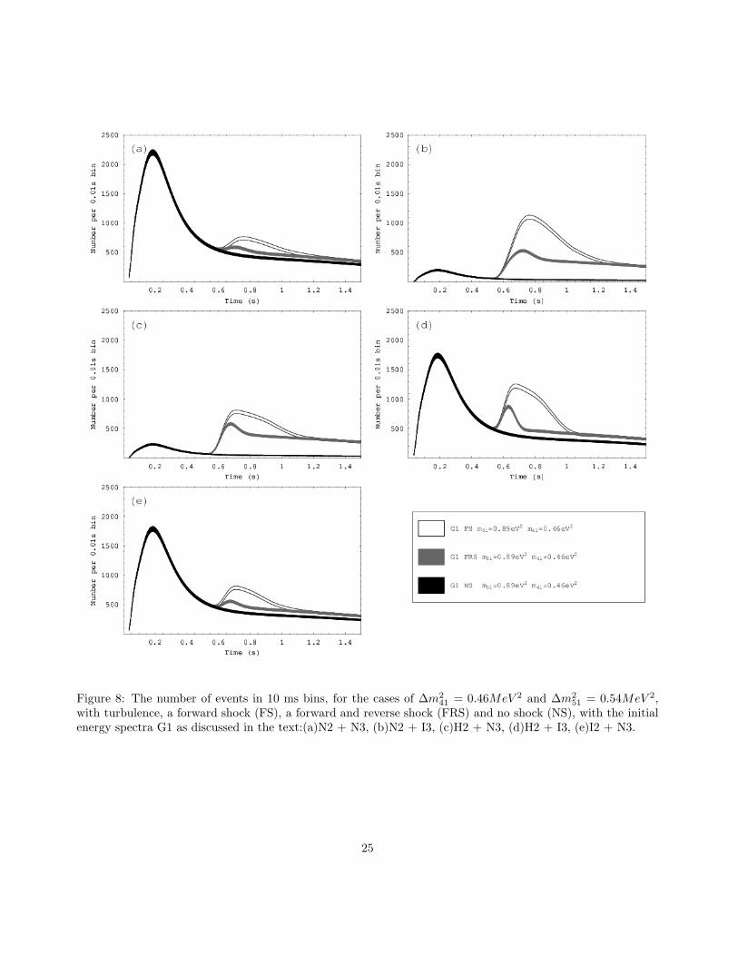
Figure 8: The number of events in 10 ms bins, for the cases of ∆m241 = 0.46MeV 2 and ∆m2

51 = 0.54MeV 2,with turbulence, a forward shock (FS), a forward and reverse shock (FRS) and no shock (NS), with the initialenergy spectra G1 as discussed in the text:(a)N2 + N3, (b)N2 + I3, (c)H2 + N3, (d)H2 + I3, (e)I2 + N3.

25

Figure 9: The average energy in 10 ms bins, for the cases of ∆m241 = 0.46MeV 2 and ∆m2

51 = 0.54MeV 2, withno turbulence, a forward shock (FS), a forward and reverse shock (FRS) and no shock (NS), with the initialenergy spectra G1 as discussed in the text:(a)N2 + N3, (b)N2 + I3, (c)H2 + N3, (d)H2 + I3, (e)I2 + N3.

26

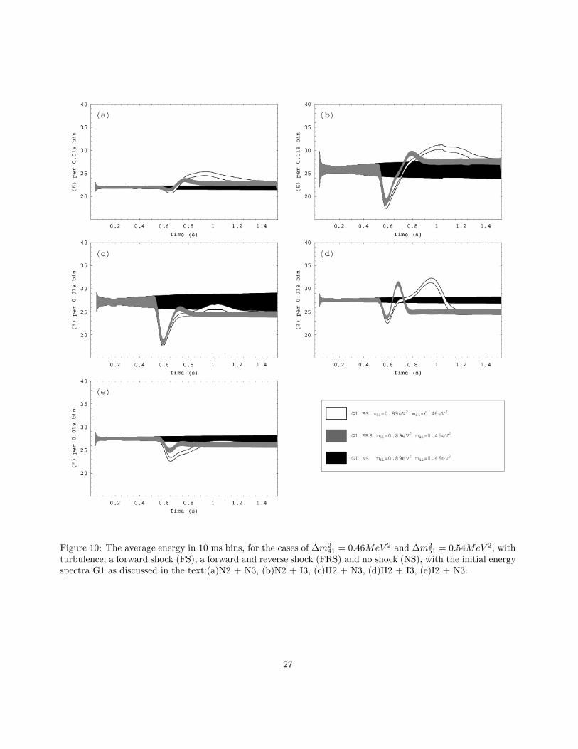
Figure 10: The average energy in 10 ms bins, for the cases of ∆m241 = 0.46MeV 2 and ∆m2

51 = 0.54MeV 2, withturbulence, a forward shock (FS), a forward and reverse shock (FRS) and no shock (NS), with the initial energyspectra G1 as discussed in the text:(a)N2 + N3, (b)N2 + I3, (c)H2 + N3, (d)H2 + I3, (e)I2 + N3.

27

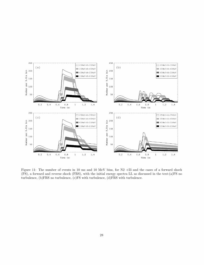
Figure 11: The number of events in 10 ms and 10 MeV bins, for N2 +I3 and the cases of a forward shock(FS), a forward and reverse shock (FRS), with the initial energy spectra LL as discussed in the text:(a)FS noturbulence, (b)FRS no turbulence, (c)FS with turbulence, (d)FRS with turbulence.

28