
TURBULENCE: THEORY AND MODELING LECTURE 6 · 2014-11-17 · TURBULENCE: THEORY AND MODELING LECTURE...
37
Wall bounded flows 2/2 TURBULENCE: THEORY AND MODELING LECTURE 6
Transcript of TURBULENCE: THEORY AND MODELING LECTURE 6 · 2014-11-17 · TURBULENCE: THEORY AND MODELING LECTURE...

Wall bounded flows 2/2
TURBULENCE: THEORY AND MODELING
LECTURE 6

Main categories
• Channel flow
• Pipe flow
• Flat plate boundary layer
• 2D
• Simplified equations can be derived
• Average velocity profile
• Reynolds stresses
• Is there any ’universal rule’ ?
• Models

Nondimensionalized governing equations (2D)
0*
*
*
*=
∂∂
+∂∂
yv
xu
*
**
*
**
2*
*2
2*
*2
*
*
*
**
*
**
*
*
Re1
Re1
yvu
xuu
y
u
x
uxp
yuv
xuu
tu
∂′′∂
−∂
′′∂−
∂
∂+
∂
∂+
∂∂
−=∂∂
+∂∂
+∂∂
*
**
*
**
2*
*2
2*
*2
*
*
*
**
*
**
*
*
Re1
Re1
yvv
xvu
y
v
x
vyp
yvv
xvu
tv
∂′′∂
−∂
′′∂−
∂
∂+
∂
∂+
∂∂
−=∂∂
+∂∂
+∂∂

Simplify • Assumptions
– Statistically stationary
– Fully developed, i.e. For velocities:
– Also:
– No * in the followings x
y
U V
xy ∂∂
>>∂∂
0=∂∂t
vu >>
δ>>L

Simplify y-momentum
yvv
xvu
yv
xv
yp
yvv
xvu
tv
∂′′∂
−∂
′′∂−
∂∂
+∂∂
+∂∂
−=∂∂
+∂∂
+∂∂
2
2
2
2
Re1
Re1
0=∂∂t xy ∂
∂>>
∂∂
( ) ( ) ( )( ) ( ) ( )δδ
δδδ kOkOO
OypOO −−++
∂∂
−=+Re
1Re
uL
vyv
xu δ
∝⇒=∂∂
+∂∂ 0
O(1)

Y-momentum
• Integrate
• Differentiate on x
P0, v’=0
0=∂
′′∂+
∂∂
yvv
yp
0ppy →⇒∞→
vvpp ′′−= 0
xvv
dxdp
xp
∂′′∂
+=∂∂ 0

2D Boundary Layer Equations
0=∂∂
+∂∂
yv
xu
yvu
yu
dxdp
yuv
xuu
∂′′∂
−∂∂
+−=∂∂
+∂∂
2
20
Re1
Using Bernoulli:
dxdUU
dxdp 0
00 =−

Special case: Fully developed channel flow
0)()( ==− hvhv
0=∂∂
yv
yvu
yu
dxdp
∂′′∂
−∂∂
= 2
20
Re1
0=v
Rewrite ( ) ( )
yydxdp xyxy
∂∂
−∂
∂=
turbvisc0 ττ i.e. the total stress is
independent of x and varies linearly with y
• Continuity:
• BCs: • X-momentum:
U
yvu
yu
dxdp
yuv
xuu
∂′′∂
−∂∂
+−=∂∂
+∂∂
2
20
Re10=
∂∂
xu

Wall shear stress Skin friction
( ) ( )
yyydxdp xyxyxy
∂
∂=
∂
∂−
∂
∂=
τττ turbvisc0
• wall shear stress antisymm.
• Normalize: friction coefficient
U
0=∂∂
xu
2δ
τw
−τw
δτ w
dxdp
=− 0
τw
−=
δττ yy w 1)(
= 2
021/ uc wf ρτ

Total shear stress near the wall

Viscous scales • Close to the wall viscosity dominates
• Wall shear stress, τw, important
• Friction velocity:
• Viscous lengthscale:
• Friction Reynolds number:
• Wall units:
ρτρτ ττ
ww uu =⇒= 2
τν
νδu
=
ν
ττ δ
δνδ
==uRe
νδτ
ν
yuyy ==+
0
100%
Viscous stresses
Reynolds stresses
Y+ 10 20 50
Re
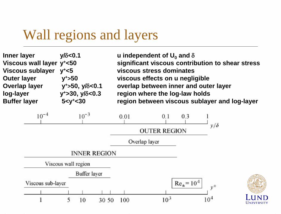
Wall regions and layers Inner layer y/δ<0.1 u independent of U0 and δ Viscous wall layer y+<50 significant viscous contribution to shear stress Viscous sublayer y+<5 viscous stress dominates Outer layer y+>50 viscous effects on u negligible Overlap layer y+>50, y/δ<0.1 overlap between inner and outer layer log-layer y+>30, y/δ<0.3 region where the log-law holds Buffer layer 5<y+<30 region between viscous sublayer and log-layer

Mean velocity profiles • We could derive u, but du/dy
appears directly in the equations
• δν – relevant lengthscale in the viscous sublayer
• δ – relevant lengthscale in the outer layer
Φ=
∂∂
δδν
τ yyy
uyu ,
( ) ( )
yydxdp xyxy
∂∂
−∂
∂=
turbvisc0 ττ
Nondimensional, unknown function
Correct units
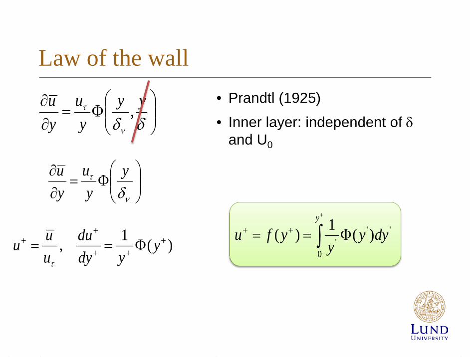
Law of the wall • Prandtl (1925) • Inner layer: independent of δ
and U0
Φ=
∂∂
δδν
τ yyy
uyu ,
Φ=
∂∂
ν
τ
δy
yu
yu
)(1, +++
++ Φ== y
ydydu
uuu
τ
∫+
Φ== ++y
dyyy
yfu0
''' )(1)(
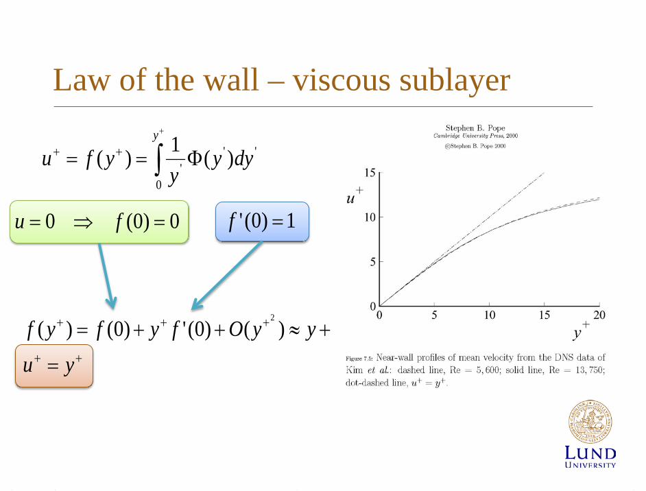
Law of the wall – viscous sublayer
0)0(0 =⇒= fu 1)0(' =f
++
+++
=
+≈++=
yuyyOfyfyf )()0(')0()(
2
∫+
Φ== ++y
dyyy
yfu0
''' )(1)(

Law of the wall – the log law • For y+>30 & y/δ << 1(still inner layer)
– Viscosity small effect
– U0 – no effect yet
– von Kármán: κ=0.41 B=5.2
– Universal, err=5%
Φ=
∂∂
δδν
τ yyy
uyu ,
Byuydy
du+=⇒= ++
++
+
ln11κκ

Velocity defect law • Outer layer, y+>50
– Viscosity neglected
– Integrate between y and δ
» u0 – centerline velocity
» FD – NOT universal
– For large Re inner and outer layers overlap
Φ=
∂∂
δδν
τ yyy
uyu ,
∫ Φ=
=
− 1
/
0 ')'('
1
δτ δ yD dyy
yyF
uuu
Log(y/δ)
(u0-u)/uτ
10 ln1 ByyFu
uuD +
−=
=
−δκδτ
Velocity-defect law for small y/δ

Friction law & Re • Inner layer
• Outer layer
10 ln1 Byu
uu+
−=
−δκτ
Byuu
+
=
ντ δκln1
NOT universal, but small
Log-law not valid, but small contribution to total mass flow.
BBuu
BBuu
++
=
++
=
−
1
1
00
10
Reln1
ln1
τ
ντ
κ
δδ
κ

Friction coefficient Outer/inner parameter ratios
BBuu
uu
++
=
−
1
1
00
0 Reln1
ττ κ
Solve for u0/uτ :
Friction coefficient:
2
0
20 2
21/
=
=
uuuc wf
τρτ
Log(Re)
cf
Laminar
Turbulent
Log(Re)
Log(δ/δν)
Log(Re)
u/uτ
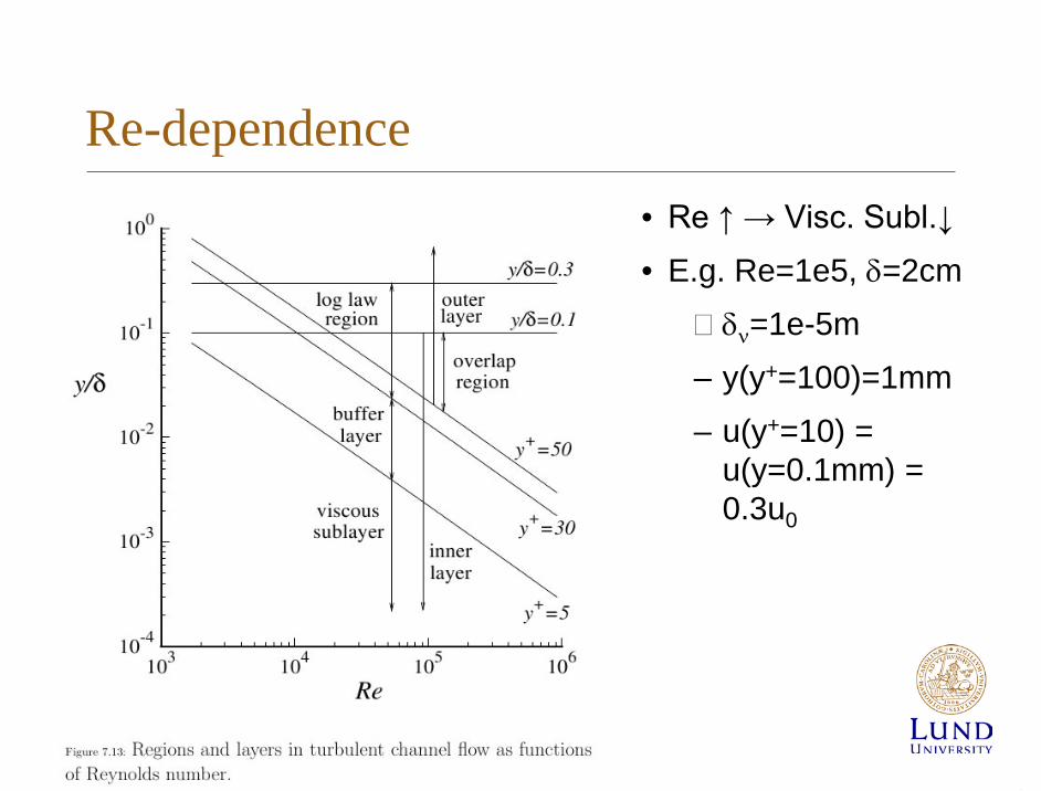
Re-dependence • Re ↑ → Visc. Subl.↓ • E.g. Re=1e5, δ=2cm
� δν=1e-5m – y(y+=100)=1mm – u(y+=10) =
u(y=0.1mm) = 0.3u0

Reynolds stresses
Y+
<ui’uj’>/k
50
<u’2>
<v’2>
<w’2>
Largest fluctuations In viscous layer Anisotropy
0

Production/dissipation, timescales
Production & dissipation almost in balance
No production on centerline
Largest production In viscous layer
1≈εP
Normalized shear stress 3.0≈
′′kvu
Time scale ratio
3≈′′
=εεP
vukSk
dyudS =
εk
Time scales:
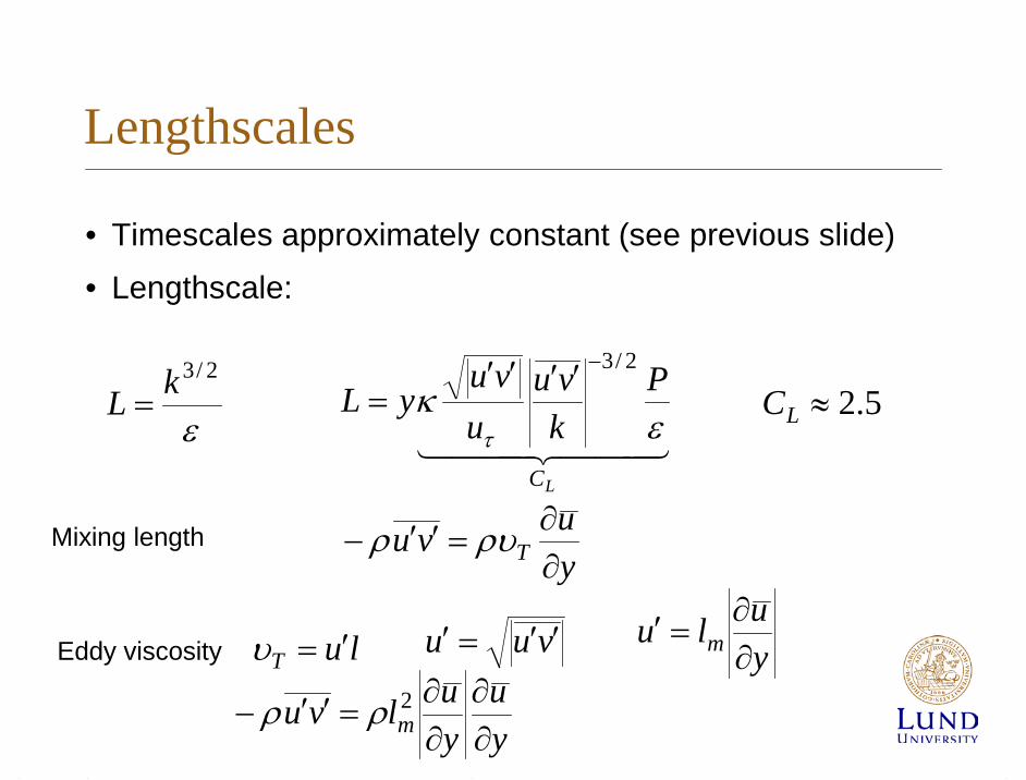
Lengthscales
• Timescales approximately constant (see previous slide) • Lengthscale:
LC
Pkvu
uvu
yLε
κτ
2/3−′′′′=
ε
2/3kL = 5.2≈LC
Eddy viscosity luT ′=υ yulu m ∂
∂=′
yu
yulvu m ∂
∂∂∂
=′′− 2ρρ
Mixing length yuvu T ∂
∂=′′− ρυρ
vuu ′′=′

Pipe flows • Similar to channel flows
• Cylindrical coordinate system
• Pipe wall roughness
• Nikuradse diagram (pp.295, Fig. 7.23)
Log(Re)
cf
Laminar
Turbulent
Roughness

Flat plate boundary layers compared to channel flow
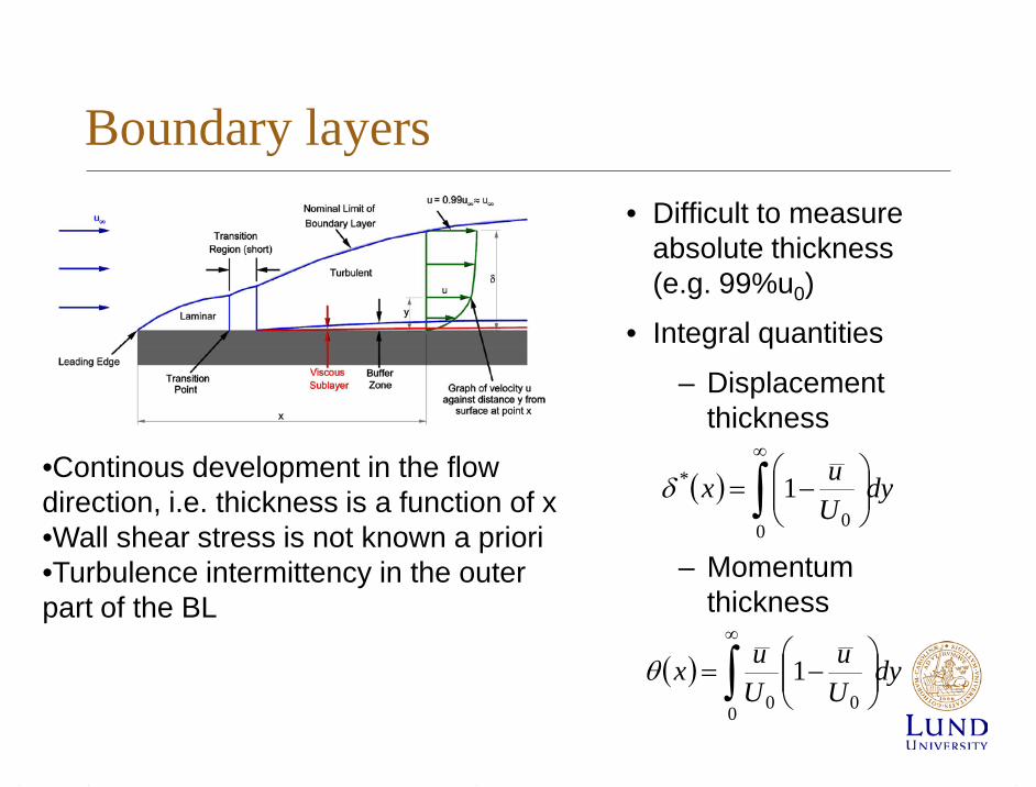
Boundary layers • Difficult to measure
absolute thickness (e.g. 99%u0)
• Integral quantities
– Displacement thickness
– Momentum thickness
•Continous development in the flow direction, i.e. thickness is a function of x •Wall shear stress is not known a priori •Turbulence intermittency in the outer part of the BL
( ) dyUux ∫
∞
−=
0 0
* 1δ
( ) dyUu
Uux ∫
∞
−=
0 001θ
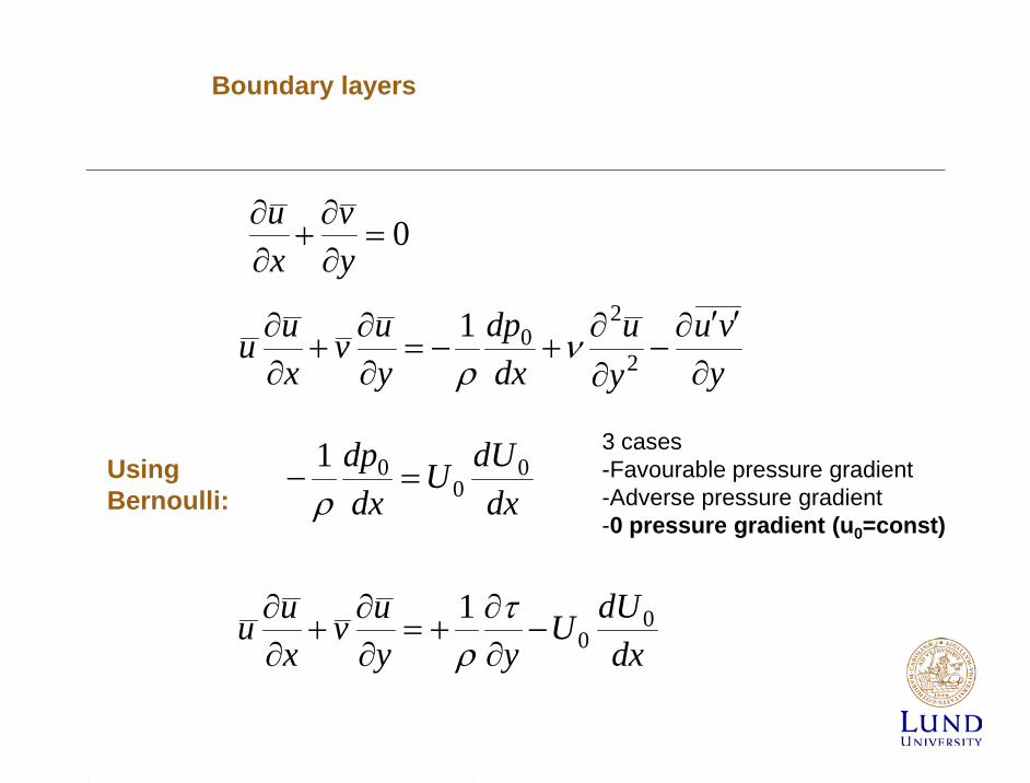
Boundary layers
0=∂∂
+∂∂
yv
xu
yvu
yu
dxdp
yuv
xuu
∂′′∂
−∂∂
+−=∂∂
+∂∂
2
201 ν
ρ
Using Bernoulli: dx
dUUdxdp 0
001
=−ρ
dxdUU
yyuv
xuu 0
01
−∂∂
+=∂∂
+∂∂ τ
ρ
3 cases -Favourable pressure gradient -Adverse pressure gradient -0 pressure gradient (u0=const)

Boundary layers
dxdUw
θρτ 20=Wall shear stress
Similarity solution by Blasius (1908) (for laminar, zero-pressure gradient)
14.0
35.0
Re9.4
*
≈
≈
≈
δθδδ
δ
xx
υxU
x0Re =
0Ux
xυδ =

( )kk
i
ik
ik
ii xx
uxp
xuu
tuuN
∂∂∂
−∂∂
+∂∂
+∂∂
=2
ν
Derivation of the transport equations for Reynolds’ stress
Introduce the ”Navier-Stokes operator”
( ) ( ) 0=′+′ jiij uNuuNu
( ) 0=iuN
After some manipulation we get
∂
′′∂−′′′
∂∂
−Π+−=∂
′′∂+
∂
′′∂
k
jikji
kijijij
k
jik
ji
xuu
uuux
Pxuu
utuu
νε

k
ikj
k
jkiij x
uuuxu
uuP∂∂′′−
∂∂
′′−=
k
j
k
iij x
uxu
∂
′∂∂
′∂= νε 2
ikj
jkip
kijpupuT δ
ρδ
ρ′′
+′′
=)(
∂
′′∂−′′′
∂∂
−Π+−=∂
′′∂+
∂
′′∂
k
jikji
kijijij
k
jik
ji
xuu
uuux
Pxuu
utuu
νε
Production tensor
Dissipation tensor
Velocity-pressure-gradient tensor
k
pkij
ijij xT
R∂
∂+=Π
)(
∂
′∂+
∂′∂′
=i
j
j
iij x
uxupR
ρPressure-rate-of-strain tensor
Pressure transport tensor
Turbulent transport Viscous
diffusion

∂
′′∂−′′′
∂∂
−Π+−=∂
′′∂+
∂′′∂
k
iikii
kiiiiii
k
iik
ii
xuu
uuux
Px
uuu
tuu 2
1
21
21
21
212
121
νε
Take trace:
∂
′′∂−′′′
∂∂
−Π+−=∂
′′∂+
∂
′′∂
k
jikji
kijijij
k
jik
ji
xuu
uuux
Pxuu
utuu
νε
∂∂
−′′
+′′′∂∂
−−=∂∂
+∂∂
k
kkii
kkk x
kpuuuux
Pxku
tk ν
ρε 2
1
Which is the equation for turbulent kinetic energy
Note: ρpuk
ii′′
=Π21 0=iiR
k
i
k
iii x
uxu
∂′∂
∂′∂
== νεε21
j
ijiii x
uuuPP∂∂′′−==2
1
Reynolds stress → TKE

yuvu
zuwu
yuvu
xuuuP
∂∂′′−=
∂∂′′−
∂∂′′−
∂∂′′−= 222211
022222 =∂∂′′−
∂∂′′−
∂∂′′−=
zvwv
yvvv
xvvuP
033 =P
Production
Production occurs in u’u’

Production balanced by dissipation. Pressure not significant.

Pressure term IS a significant sink term!

Pressure term is a significant source term! Redistribution Important @ modeling!
ikj
jkip
kijpupuT δ
ρδ
ρ′′
+′′
=)(
∂
′∂+
∂′∂′
=i
j
j
iij x
uxupR
ρ


