Turbo Machines

Ramesh K

November 14, 2012

1 Introduction to Turbo Machines

1.1 Introduction

Turbomachine is important class of fluid machine, which has as its characteristic theability to transfer energy continuously between a dynamic fluid and a mechanical elementrotating around a fixed axis. The definition of turbo-machine as given by different authors

• The Turbo-machine is a device in which the energy exchange is accomplished byhydrodynamic forces arising between moving fluid and the rotating and stationaryelements of the machine - Daily.

• A Turbo-machine is characterized by dynamic energy exchange between one or sev-eral rotating elements and a rapidly moving fluid - Wislicenus.

• A Turbo-machine is characterized by dynamic action between a fluid and one ormore rotating elements - Binder.

As we can see that the study of turbo-machine comprises of fluid motion in relative to amoving mechanical elements. When ever some body/fluid is in motion either forces act onthem or the motion is the result of forces being acted upon the body/fluid. The resultantof forces acting result in energy transfer to/from the fluid to the machine. Hence theessential prerequisite of this course is knowledge/awareness in

• Fluid Dynamics (Incompressible and Compressible fluid flows)

• Vector Algebra and Calculus

• Theory of Machines (Kinetics and Kinematics)

• Basic and Applied Thermodynamics

Some of the application areas where in we use turbo-machines

• Propulsion systems - Aircraft,Marine, Space(Liquid rockets) and Land propulsionsystems

• Power generation - Steam ,gas and hydraulic turbines

• Industrial pipe line and processing equipments such as gas, petroleum and waterpumping plants

• Heart assist pumps, industrial compressors and refrigeration plants

1

So what do we do in this course?We will try to

• Unleash the basic terminology of the turbo-machine.

• Understand the basic working of a turbo-machine irrespective of its use.

• Understand the performance parameters of its effects on a turbo-machine.

2 Classification of Turbo Machines

There are many categories in which a turbo-machine is classified

2.1 Direction of Energy Conversion

• Turbine- It is a machine where the energy in the fluid in what ever the form (KineticEnergy, Potential Energy or Internal Energy) is converted to mechanical energy byrotating a element(rotor) of the machine.The energy is being extracted from the fluid in the form of shaft power by decreasingits enthalpy, hence they are also called power generating machines.

• Pump - In these kind of machines, mechanical energy in the rotating member istransferred to the fluid raising its energy (enthalpy) in the form of (KE, PE or IE).Since energy is gained by the fluid they are called power consuming machines.Fans, blowers, compressors etc also fall in this category.

2.2 Components of Turbo-machine

• Casing - Outer enclosing of the machine used to stop spill over of the fluid and alsoserves as guide.

• Runner - Also called ”Rotor”, where in actual energy transfer from the fluid or to thefluid takes place. It changes the stagnation enthalpy,Kinetic energy and stagnationpressure field of the fluid.

• Blades - Also called as ”Vanes”, which are use to extract or take energy from thefluid.

• Draft tube - A pipe at the exit of the machine used to maintain the energy loss andcontinuity at the exit of the machine.

If the turbo-machine doesn’t have shroud or annulus wall near the tip, then the machineis called extended. Examples of such machines are aircraft and ship propellers, windturbines, fans. Other way around if they have shroud or enclosure then they are calledenclosed machines.

2

(a) Pelton Wheel (b) Kaplan Turbine

Figure 1: Turbo machines, Images courtesy World Wide Web

2.3 Principle of Operation

• Positive Displacement Machine - As the name suggests, the functioning ofthese machines depends on the physical change in the volume of the fluid within themachine.The name positive displacement is given as the fluid in the machine forms a closedsystem and the boundary of the system is physically displaced as in piston cylinderarrangement as shown in the Piston cylinder Figure (2a), Gear pump Figure (2b),screw pump Figure (2c). Since the motion of the piston is reciprocating (to and

(a) Reciprocating pump/machine (b) Gear Pump (c) Screw Pump

Figure 2: Positive Displacement machines, Images b &c courtesy World Wide Web

fro linear motion), these machines are also known as reciprocating engines. If themachine used is for generating power then it is called as Internal combustion engineother wise if used for compression of gas it is called reciprocating pump. Gear pumpsand screw pumps also fall in the category of positive displacement pumps thoughthere is no reciprocating action involved.

• Roto Dynamic machine - In this kind of machine both thermodynamic anddynamic interaction between the flowing fluid and the rotating element takes placeand involves energy transfer with change in both pressure and momentum. Thesemachines are distinguished from positive displacement machines in requiring that

3

there exists a relative motion between the flowing fluid and rotating element. Therotating element usually consists of blades/vanes which are used to transfer theenergy and also aids the fluid to flow in a particular direction.

2.4 Direction of flow

• Radial - Fluid is in the direction perpendicular to the axis of the rotating elementand leaves radially.

• Axial - Flow enters parallel to the axis of the rotating element and leaves axially.

• Mixed - Fluid enters radially or axially and leaves axially or radially.

2.5 Types of Fluids used

• Gas or Vapour - Air,Argon,Neon,Helium,Freon,Steam,Hidrocarbon gas etc,.

• Liquid - Water, Cryogenic liquids (O2, H2, F2, NH2etc, .), Hydrocarbon Fuels, Slurry(Two Phase liquid/solid mixture),Blood, Potassium,Mercury etc

4

2.6 Examples where Turbo-machines are used

Field Name Turbine Pump or Compres-sor

Application area

Aerospace Vehicleapplication

Gas Turbines Compressors,Pumps,Propellers • Power and propulsion of aircrafts

• Helicopters, UAV,V/STOL aircrafts Mis-siles

• Liquid rocket engines

Marine applica-tions

Gas Turbinesand Turbines

Compressors,Pumps,Propellers • Power and propulsion for submarines

• Hydrofoil boats, Naval surface ships, Hov-ercrafts

• Underwater vehicles

Land Vehicle appli-cation

Gas Turbinesand Turbines

Centrifugal com-pressor and radialturbine

Trucks,cars and high speed trains

Energy application Gas,Steam andwind Turbines

Compressors,Pumps

• Hydraulic turbines in hydro-power plants

• Gas turbine power plants

Industrial applica-tions

Compressors,Pumps • Compressors - Transport of Petroleum

and other processing applications

• Pumps - Fire fighting, water purification,pumping plants

• Refrigeration - High speed miniatureturbo expanders

Miscellaneous Pumps Heart assist devices(artificial heart pump), auto-motive torque converters, swimming pools, hy-draulic brakes

Looking at wide area of application of turbo-machines, any small gain in performance andefficiency of a turbo-machine would impact the economy globally.

2.7 Nature of flow field

It is complex 3D flow field that exist in any turbo-machine. A typical example of flow field thatexist is as shown in figure

2.7.1 Fluid Used

By the nature of the fluid used they can be classified as compressible and incompressible

5

(a) Axial flow type machines (b) Centrifugal flow type machines

Figure 3: 3D Flow Field in any turbo-machine-Image courtesy - Budugur Lakshmi-narayana(Fluid dynamics and heat transfer in turomachinery)

• Compressible - If the changes in the pressure caused by the fluid motion results in changesin density of the fluid then such type of fluid is known to be a compressible fluid. In agiven turbo-machine since pressure changes are inevitable and if accompanied by densitychanges then it is under the category of compressible flow turbo-machine. Gas turbines,air compressors etc fall in this category. The flow in compressible machines may be furtherclassified into

(a) Compressible Type Turbo-machine

(b) Incompressible type Turbo-machine

Figure 4: Turbo machines, Images courtesy World Wide Web

– Subsonic - M ≤ 0.7

– Transonic -0.7 ≤M ≤ 1.0

– Supersonic -M ≥ 1.0

• Incompressible -If the changes in the pressure doesn’t affect much of the density changesthen they are considered to be incompressible flow turbo-machines. Steam turbine andall hydraulic turbines fall in this category.

2.7.2 Kinds of flow

• Steady - If the fluid properties doesn’t vary in time.

• Unsteady- Fluid properties vary in time.

6

Figure 5: Turbo machines- Impulse and Reaction types, Images courtesy World WideWeb

2.8 Type of forces acting

• Impulse type - Static Pressure change is zero in the rotor.

• Reaction type - Static Pressure drop occurs in the rotor.

7

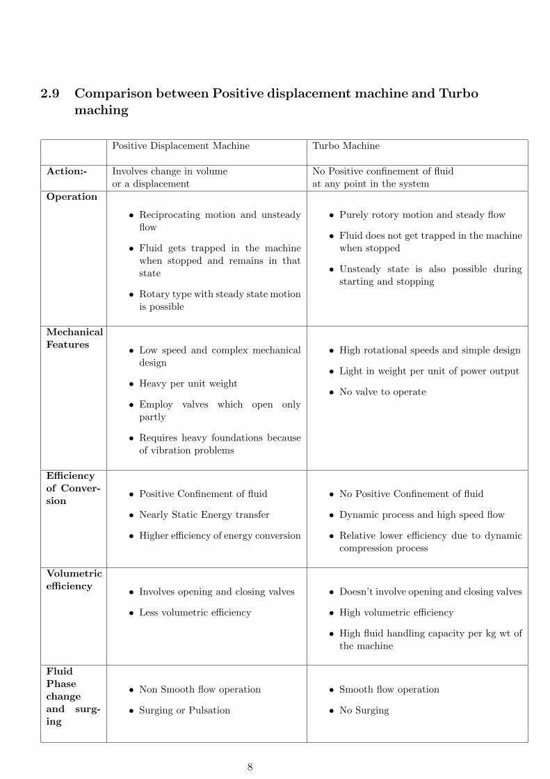
2.9 Comparison between Positive displacement machine and Turbomaching

Positive Displacement Machine Turbo Machine

Action:- Involves change in volume No Positive confinement of fluidor a displacement at any point in the system

Operation

• Reciprocating motion and unsteadyflow

• Fluid gets trapped in the machinewhen stopped and remains in thatstate

• Rotary type with steady state motionis possible

• Purely rotory motion and steady flow

• Fluid does not get trapped in the machinewhen stopped

• Unsteady state is also possible duringstarting and stopping

MechanicalFeatures • Low speed and complex mechanical

design

• Heavy per unit weight

• Employ valves which open onlypartly

• Requires heavy foundations becauseof vibration problems

• High rotational speeds and simple design

• Light in weight per unit of power output

• No valve to operate

Efficiencyof Conver-sion

• Positive Confinement of fluid

• Nearly Static Energy transfer

• Higher efficiency of energy conversion

• No Positive Confinement of fluid

• Dynamic process and high speed flow

• Relative lower efficiency due to dynamiccompression process

Volumetricefficiency • Involves opening and closing valves

• Less volumetric efficiency

• Doesn’t involve opening and closing valves

• High volumetric efficiency

• High fluid handling capacity per kg wt ofthe machine

FluidPhasechangeand surg-ing

• Non Smooth flow operation

• Surging or Pulsation

• Smooth flow operation

• No Surging

8

3 Basics of Fluid Mechanics and Thermodynamics

It can be viewed that this subject of turbo-machinery is truly interdisciplinary as depicted in thefollowing picture. In this section the basic governing laws of fluid mechanics and thermodynamics

Figure 6: Inter diciplenary nature of the subject Turbomachinery

as applied to a turbo-machine is explained. Since the governing equations are Navier-Stokesequations and they are non-linear in nature, the complete 3D solution to the equations are outof the scope of this introductory course. A general form of the governing equations are explainedin this section and further reductions to 1D cases are followed for each case.Let us consider a turbo-machine enclosed in a control volume (Open system in thermodynamic

sense) of volume Ω as shown in Figure 7, let ”dS” be elemental surface area with unit outwardnormal to the surface n. Let ~V be the velocity with which the fluid is coming out of the surfaceelement ”dS”. Let min & mout, be the mass flow rates in and out of the control volume, alsoQin & Qout be the rate at which heat is transferred into or out of the control volume.The properties which we are interested in analyzing a turbo-machine vary both in space and time(i.e, as the fluid moves through the turbo-machine). If we denote φ(x, y, z, t) as the property

9

Figure 7: Control volume enclosing a turbo-machine

which is varying with both Cartesian spatial coordinates (x, y, z) and ”t”, then

dφ =∂φ

∂tdt+

∂φ

∂xdx+

∂φ

∂ydy +

∂φ

∂zdz (3.1)

dφ =∂φ

∂tdt+∇φ · d~r (3.2)

∇ =∂()

∂xı+

∂()

∂y+

∂()

∂zk (3.3)

~r = xı+ y+ zk (3.4)

d~r = dxı+ dy+ dzk (3.5)

dφ

dt=∂φ

∂t+∇φ · ~V (3.6)

where equation (3.3) represents the gradient operator being operated on any property. Theproperty φ can be a scalar, vector or a tensor. Total rate at which the property changes isgiven in equation (3.6), which has two parts the fist part indicating the local rate at whichthe property is changing with respective to time and the second term represents the rate atwhich the property is changing from one point to other inside the control volume, also called asconvective part.This gradient when applied to a scalar results in a vector, when applied to a vector results in asecond order tensor and when applied to a second order tensor results in a higher order tensor.Let us consider the gradient operator applied to a velocity vector ~V (~r, t) = u(~r, t)ı + v(~r, t) +w(~r, t)k, all the individual components of this vector are varying w.r.t space as well as time.

∇(~V ) =∂(~V )

∂xı+

∂(~V )

∂y+

∂(~V )

∂zk (3.7)

=∂(u(~r, t)ı+ v(~r, t)+ w(~r, t)k)

∂xı +

∂(u(~r, t)ı+ v(~r, t)+ w(~r, t)k)

∂y

+∂(u(~r, t)ı+ v(~r, t)+ w(~r, t)k)

∂zk

=

(∂u

∂xıı+

∂u

∂yı+

∂u

∂zık

)+

(∂v

∂xı+

∂v

∂y+

∂v

∂zk

)(3.8)

+

(∂w

∂xkı+

∂w

∂yk+

∂v

∂zkk

)10

equation(3.7) contains ”9” components as shown in equation(3.8), and each component has 2directions associated with it. Thus it can be observed that gradient operator increases the orderby one. The other operator of importance is the divergence operator given by ∇() · ( ~A), it isthe dot product or scalar product of the gradient operator with any vector or a tensor. As it isknown that the dot product of two vectors results in a scalar since the ∇() is a vector quantity,when taken a dot product with any vector or a tensor will result in a scalar or a vector reducingthe order.

∇() · ~V =

(∂()

∂xı+

∂()

∂y+

∂()

∂zk

)·(uı+ v+ wk

)(3.9)

=

(∂(u)

∂x+∂(v)

∂y+∂(w)

∂z

)(3.10)

The cross product of the gradient operator applied to the velocity vector results in a vectorwhich signifies the linear and angular strain rates of the fluid element as it moves through thefluid

∇()× ~V =

(∂()

∂xı+

∂()

∂y+

∂()

∂zk

)×(uı+ v+ wk

)(3.11)

=

(∂(w)

∂y− ∂(v)

∂z

)ı−(∂(w)

∂x− ∂(u)

∂z

)+

(∂(u)

∂y− ∂(v)

∂x

)k (3.12)

Equation 3.12, gives the rotation of the fluid element as it traverses through the control volume.The Gauss-Divergence theorem gives the relation between the volume integral of a divergenceand the surface integral of the vector as given by∫

Ω

(∇ · ~A

)dΩ =

∮S

~A · ndS (3.13)

This equation (3.13) represents the divergence of the vector quantity inside the control volumeto the flux of the quantity passing through the surface.

3.1 Conservation of Mass or Continuity equation

”Mass is neither created nor destroyed”, or in other words,”The sum of rate of change of massinside the control volume and the net mass flux from the control surface is zero”.

d

dt

∫ΩρdΩ +

∮Sρ~V · ndS = 0 (3.14)

d

dt

∫ΩρdΩ +

∫Ω∇.(ρ~V)dΩ = 0 (3.15)

∂ρ

∂t+∂ρvi∂xi

= 0, i = 1, 2, 3 (3.16)

Equation (3.14) represents the conservation of mass as applied to a control volume (open system),using Gauss-Divergence theorem, converting the second term in (3.14), surface integral to volumeintegral results in eq (3.16) which is valid at any given point inside the control volume includingthe boundaries. The first term in the above equations is the time rate of change of mass in sidedthe control volume or at a point and the second term the net mass flux (mass flux coming inand mass flux going out) crossing the boundaries. For 1D case with constant control volumeequation (3.14) reduces to

dρ

dtΩ +

∑i

(ρA(v1 · ı))i = 0 (3.17)

dρ

dtΩ−

∑inlet

(ρAv1)inlet +∑outlet

(ρAv1)outlet = 0 (3.18)

11

In the case of steady flow the first term in eq (3.17) is zero, meaning that the the ”mass fluxentering the control volume is equal to mass flux leaving the control volume”. The equation forcontinuity or mass conservation for 1D stead flow is given by eq (3.18)∑

i

(ρA(v1 · ı))i = 0 (3.19)

−∑inlet

(ρAv1)inlet +∑outlet

(ρAv1)outlet = 0 (3.20)∑inlet

(ρAv1)inlet =∑outlet

(ρAv1)outlet (3.21)

3.2 Conservation of Linear Momentum

Newtons second law of motion says, ”The rate of change of linear momentum is equal to thenet force acting on a body”. From engineering mechanics or physics point of view for particlebodies, the Newtons second law is given by

d(m ~V)

dt=∑i

~Fi (3.22)

where the summation indicates all the forces acting on the body and the right hand side indi-cating the time rate of change of linear momentum. In the integral form as applied to a controlvolume the equation (3.22) takes the form as given in equation (3.23)

d

dt

∫Ωρ~V dΩ +

∫∂Ω

(ρ~V )~V · n dS = −∫∂ΩPn dS +

∫Ωρ~gdΩ +

∫∂Ωτ.ndS (3.23)

d

dt

∫Ωρ~V dΩ +

∫Ω∇ ·(

(ρ~V )~V)dΩ = −

∫Ω∇.(Pn)dΩ +

∫Ωρ~gdΩ +

∫Ω∇ · τdΩ (3.24)

In the equation (3.23) the surface integrals are converted to volume integrals by using Gauss-Divergence theorem. The forces considered in the present context are pressure forces (surfaceforce st term), gravity force (body force nd term) and viscous forces (surface force rd term).If the surface is further divided into discrete elemental surfaces then the equation (3.23) can berewritten as given in equation (3.25)

d

dt

∫Ωρ~V dΩ +

∑i

(ρ~V S)(~V · n)i = −∑i

(PnS)i + ρ~gΩ +∑i

(τ.nS)i (3.25)

d

dt

∫Ωρ~V dΩ +

∑i

(m)(~V · n)i = −∑i

(PnS)i + ρ~gΩ +∑i

(τ.nS)i (3.26)

The negative sign in the st term on RHS indicating that the force due to the pressure isof compressive in nature. The second term on LHS is the momentum flux that is crossingthe surface, the momentum that is carried away by the fluid from the control volume. Thesummation indicates the momentum flux that is entering the control volume and the also leavingthe control volume. This aspect of inlet or exit of momentum form the control volume is taken

care by the the(~V · n

)term in the above equation. If this term is positive

(~V · n > 0

)then

the flux is moving out and if its negative(~V · n < 0

)it is flowing in.

For a steady state, inviscid with negligible body forces, the momentum equation (3.26) reducesto ∑

i

(m)(~V · n)i = −∑i

(PnS)i (3.27)

which is the summation of momentum flux on the control volume equals the net pressure forceacting on the control volume and the momentum variation inside the control volume is fixed.

12

3.3 Conservation of Angular Momentum

The equation for the conservation of angular momentum equation is obtained by taking themoment of the momentum by the position vector.

~r × d(m ~V)

dt= ~r ×

∑i

~Fi (3.28)

d(~r × (m ~V))

dt=∑i

(~r × ~F

)i

(3.29)

d(H)

dt=∑i

Ti (3.30)

From the control volume analysis of the linear momentum equations (3.23 & 3.24), by takingthe moment w.r.t the position vector ~r, results in the integral form of the angular momentumequation as applied to a control volume.

d

dt

∫Ω~r × ρ~V dΩ +

∫S~r × (ρ~V )~V · n dS = −

∫S~r × Pn dS +

∫Ω~r × ρ~gdΩ +

∫S~r × τ.ndS(3.31)

d

dt

∫Ω~r × ρ~V dΩ +

∑i

(~r × (ρ~V )

(~V · n S

))i

= −∑i

(~r × PnS)i + ~r × (ρ~gΩ) +∑i

(~r × τ.nS)i(3.32)

for steady state cases with only pressure forces being acting on the control volume the equation(3.32) reduces to ∑

i

(~r × (ρ~V )

(~V · n S

))i

= −∑i

(~r × PnS)i (3.33)

3.4 Conservation of Energy or First law of Thermodynamics

”Energy is neither created nor destroyed, but is converted from one form to another”, validwhen relativistic effects are not taken into consideration and no nuclear reactions occur in theprocess.

Et = e+V 2

2+ gz (3.34)

d

dt

∫Ω

(ρEt)dΩ +

∮S

(ρEt)(~V · ndS) = −∮S

(P ~V · ndS) +

∮S~q · ndS +

∮S

(τ · ~V ) · ndS(3.35)

In equation (3.35) is valid for a 3D arbitrary fixed control volume, the 1st is the rate of changeof total energy inside control volume, 2nd is the energy flux crossing the boundary and also thework done by the pressure at the boundary, 3rd term represents the heat transfer by conductionat the boundaries and the last term represents the work done by viscous stress at the boundary.For steady state conditions the first term in the equation (3.35) becomes zero and the net energybalance is due to the energy flux transfer across the boundaries and the amount of heat andwork transfer across the boundaries. If this equation (3.35), is rewritten for a 1D steady statecase ∮

S(ρEt + P )(~V · ndS) =

∮S~q · ndS +

∮S

(τ · ~V ) · ndS (3.36)∑i

(ρEtv1S + Pv1S)i −∑i

(q1S)i −∑i

τijvjSi = 0, j = 1, 2, 3 (3.37)∑i

(ρEtv1) =∑i

(q1)i − Pv1 +W (3.38)∑i

(ρEtv1) =∑i

(q1)i −∑i

Wi (3.39)

∆U = δQ− δW (3.40)

13

4 Static and Stagnation Properties

The properties (like pressure, temperature) that are measured by the instruments which movewith the velocity of the fluid in motion are called static properties. If we consider an adiabaticsystem with no shaft work done on/by the system and zero potential then from the first law perunit mass applied to the control volume results in eq(4.5)

dq = dEt + dw (4.1)

dq = dEt + dws (4.2)

dEt = 0⇒ Et2 − Et1 = 0 (4.3)

Et = h+V 2

2+ gz (4.4)

h1 +V 2

1

2= h2 +

V 22

2(4.5)

If we now assume that at any given point, if we hypothetically bring the fluid particle to resti.e.,(V2 is made zero) under the assumptions that, there is no transfer of heat and no work done,also further assumed that there are no irreversibilities that arise during this process (meaningto say that, the hypothetical process is isentropic) then we can deduce from eq(4.5) that

h1 +V 2

1

2= h2 (4.6)

h = cpT ⇒ cpT1 +V 2

1

2= cpT2 (4.7)

T1 +V 2

1

2cp= T2 (4.8)

This state obtained is called stagnation property. Remember that this is an hypothetical processwhich may or may not occur in the real processes. Also this process is assumed to occur at allthe points inside the flow field. Hence at every point in the flow field if we can measure a staticproperty then corresponding to that point it is possible to obtain a corresponding stagnationproperty for all the measurable properties. Stagnation properties are also called total propertiesand are designated by the symbols subscripted with “o” or “t” as given Po, Tt, Pt, To. It is theconvenience that the use of ”o” or ”t” is used.

5 Application of Conservation Laws

5.1 Flow through nozzles and diffusers

Understanding flow through a nozzle and diffuser will be of great help in understanding theflow through turbo-machine. Let Po be the atmospheric pressure that is acting on the nozzleas shown in figure 8, similarly the pressure can assume the pressure distribution on the diffuseralso. The forces acting are the pressure, viscous forces and intertial forces. Body forces due tothe gravity are neglected. Assuming steady flow through the nozzle or diffuser and applyingthe conservation equations of mass and momentum to the control volume abcd we obtain the

14

Figure 8: Control volume enclosing a Nozzle and a Diffuser

following equations. Mass Conservation equation as applied to nozzle or diffuser results in∫Sρ~V · ndS = 0 (5.1)∫ b

aρ~V · ndS +

∫ c

bρ~V · ndS +

∫ d

cρ~V · ndS +

∫ a

dρ~V · ndS = 0 (5.2)∫ b

aρ~V · ndS +

∫ d

cρ~V · ndS = 0 (5.3)

− (ρVnS)inlet + (ρVnS)outlet = 0 (5.4)

(ρVnS)inlet = (ρVnS)outlet (5.5)

minlet = moutlet, Mass flow rate (5.6)

Qinlet = Qoutlet, Discharge- Volume flow rate (5.7)

where Vn = ~V · n is the normal Velocity vector at the surface under consideration. From thegeometry shown in Figure 8 it can be observed that Sab > Scd, further if ρ remains constantor there is no considerable change then the V1 < V2 for the nozzle and the case would be quiteopposite in the case of diffuser. The above statements are valid if the flow is subsonic case.The momentum conservation equation eq(3.23) as applied for the flow through nozzle with nobody and viscous forces is given as ∫

(ρ~V )(~V · n)dS = −∫

(PndS) + ~F(5.8)∫ b

a(ρ~V )(~V · n)dS +

∫ c

b(ρ~V )(~V · n)dS +

∫ d

c(ρ~V )(~V · n)dS +

∫ a

d(ρ~V )(~V · n)dS =

−∫ b

a(PndS)−

∫ c

b(PndS)−

∫ d

c(PndS)−

∫ a

d(PndS) + ~F (5.9)∫ b

a(ρ~V )(~V · n)dS +

∫ d

c(ρ~V )(~V · n)dS = −

∫ b

a(PndS)−

∫ d

c(PndS) + ~F (5.10)

The Contribution from the atmospheric pressure and the momentum exchange gets cancelledout on the surfaces b-c and d-a of the nozzle as can be seen from eq (5.9) because the pressureforces are equal and in opposite in direction and the velocity through the surfaces are zero.

15

Though the pressure on the surfaces a-b and c-d is equal to the atmospheric, since the area isnot the same, force exists because of this difference. The ~F in the above equation eq(5.9) canbe cosisdered as the one which results in holding the nozzle or the diffuser. Equation (5.9) canbe rewritten in component form as

−(ρVnSab)uab + (ρVnScd)ucd = P (Sab − Scd) + Fx (5.11)

−(ρVnSab)v + (ρv)(Vn)Scd = Fy (5.12)

−mabuab + mcducd = P (Sab − Scd) + Fx (5.13)

The v-component of the velocity is zero the force in y direction is zero. This kind of flow canbe seen in the case of fluid flowing through the blades in a turbine or compressors or pumps.

5.2 Flow on Blade passages with out blade motion

Consider a case where in the fluid flows on a blade passage. The following assumptions areconsidered in this case,

• Steady flow

• Fluid is inviscid and incompressible

• No Body forces

• Inlet and exit areas are equal

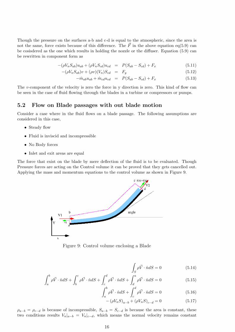
The force that exist on the blade by mere deflection of the fluid is to be evaluated. ThoughPressure forces are acting on the Control volume it can be proved that they gets cancelled out.Applying the mass and momentum equations to the control volume as shown in Figure 9.

Figure 9: Control volume enclosing a Blade

∫Sρ~V · ndS = 0 (5.14)∫ b

aρ~V · ndS +

∫ c

bρ~V · ndS +

∫ d

cρ~V · ndS +

∫ a

dρ~V · ndS = 0 (5.15)∫ b

aρ~V · ndS +

∫ d

cρ~V · ndS = 0 (5.16)

− (ρVnS)a−b + (ρVnS)c−d = 0 (5.17)

ρa−b = ρc−d is because of incompressible, Sa−b = Sc−d is because the area is constant, thesetwo conditions results Vn|a−b = Vn|c−d, which means the normal velocity remains constant

16

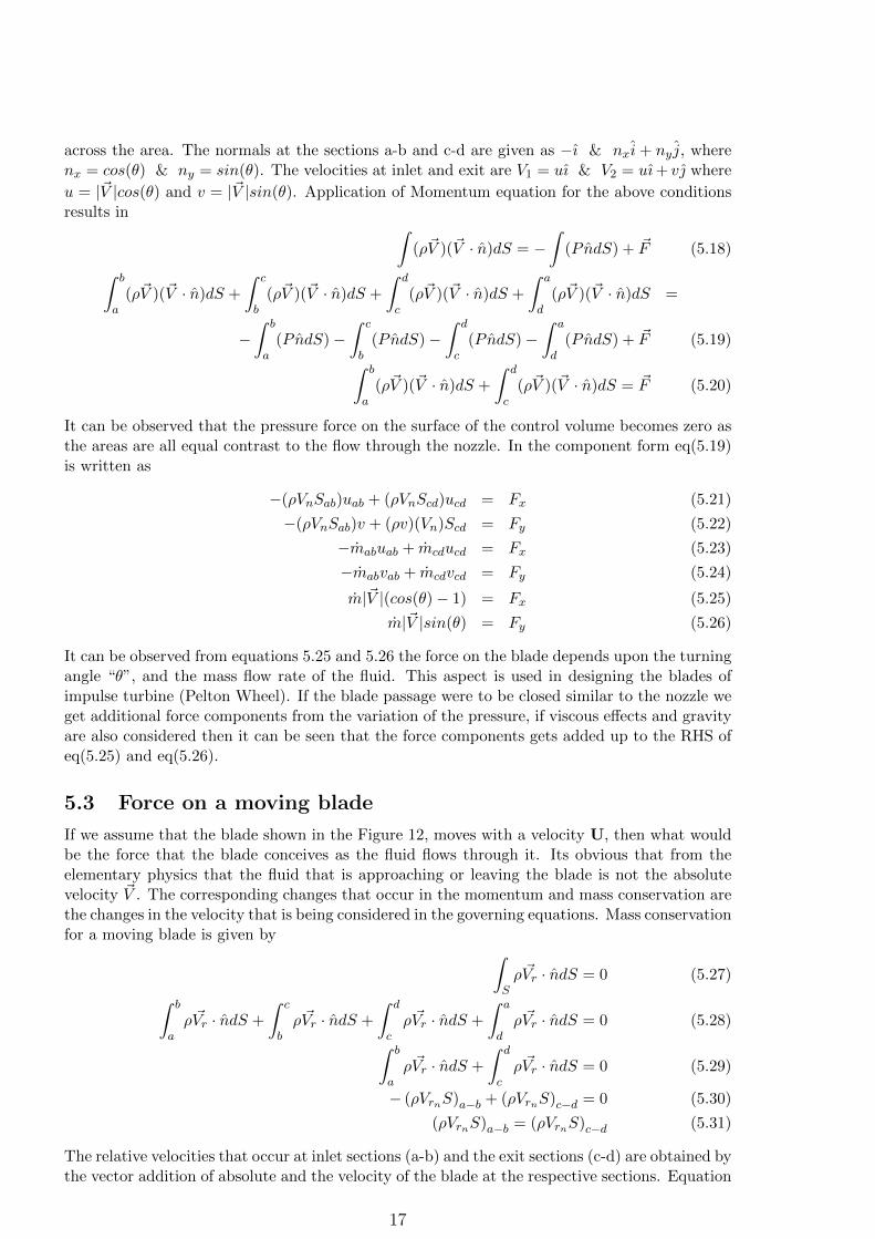
across the area. The normals at the sections a-b and c-d are given as −ı & nxi + ny j, wherenx = cos(θ) & ny = sin(θ). The velocities at inlet and exit are V1 = uı & V2 = uı+ v where

u = |~V |cos(θ) and v = |~V |sin(θ). Application of Momentum equation for the above conditionsresults in ∫

(ρ~V )(~V · n)dS = −∫

(PndS) + ~F (5.18)∫ b

a(ρ~V )(~V · n)dS +

∫ c

b(ρ~V )(~V · n)dS +

∫ d

c(ρ~V )(~V · n)dS +

∫ a

d(ρ~V )(~V · n)dS =

−∫ b

a(PndS)−

∫ c

b(PndS)−

∫ d

c(PndS)−

∫ a

d(PndS) + ~F (5.19)∫ b

a(ρ~V )(~V · n)dS +

∫ d

c(ρ~V )(~V · n)dS = ~F (5.20)

It can be observed that the pressure force on the surface of the control volume becomes zero asthe areas are all equal contrast to the flow through the nozzle. In the component form eq(5.19)is written as

−(ρVnSab)uab + (ρVnScd)ucd = Fx (5.21)

−(ρVnSab)v + (ρv)(Vn)Scd = Fy (5.22)

−mabuab + mcducd = Fx (5.23)

−mabvab + mcdvcd = Fy (5.24)

m|~V |(cos(θ)− 1) = Fx (5.25)

m|~V |sin(θ) = Fy (5.26)

It can be observed from equations 5.25 and 5.26 the force on the blade depends upon the turningangle “θ”, and the mass flow rate of the fluid. This aspect is used in designing the blades ofimpulse turbine (Pelton Wheel). If the blade passage were to be closed similar to the nozzle weget additional force components from the variation of the pressure, if viscous effects and gravityare also considered then it can be seen that the force components gets added up to the RHS ofeq(5.25) and eq(5.26).

5.3 Force on a moving blade

If we assume that the blade shown in the Figure 12, moves with a velocity U, then what wouldbe the force that the blade conceives as the fluid flows through it. Its obvious that from theelementary physics that the fluid that is approaching or leaving the blade is not the absolutevelocity ~V . The corresponding changes that occur in the momentum and mass conservation arethe changes in the velocity that is being considered in the governing equations. Mass conservationfor a moving blade is given by ∫

Sρ ~Vr · ndS = 0 (5.27)∫ b

aρ ~Vr · ndS +

∫ c

bρ ~Vr · ndS +

∫ d

cρ ~Vr · ndS +

∫ a

dρ ~Vr · ndS = 0 (5.28)∫ b

aρ ~Vr · ndS +

∫ d

cρ ~Vr · ndS = 0 (5.29)

− (ρVrnS)a−b + (ρVrnS)c−d = 0 (5.30)

(ρVrnS)a−b = (ρVrnS)c−d (5.31)

The relative velocities that occur at inlet sections (a-b) and the exit sections (c-d) are obtained bythe vector addition of absolute and the velocity of the blade at the respective sections. Equation

17

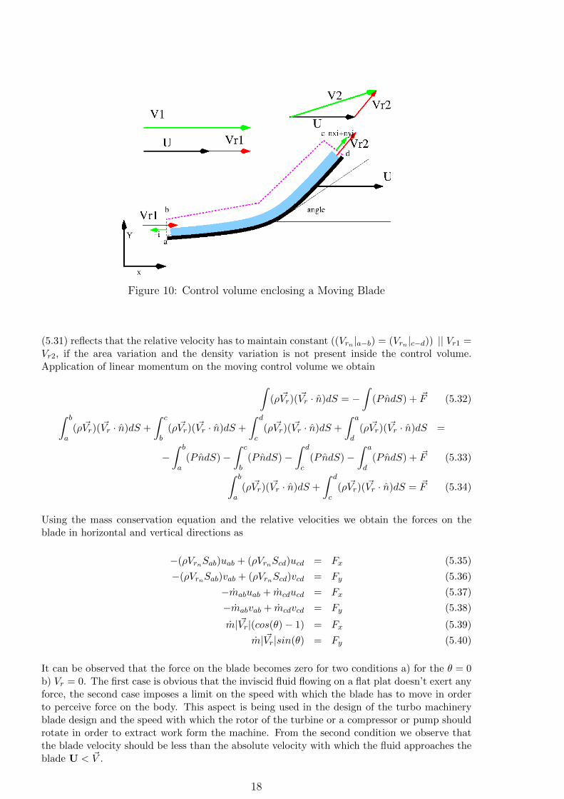
Figure 10: Control volume enclosing a Moving Blade

(5.31) reflects that the relative velocity has to maintain constant ((Vrn |a−b) = (Vrn |c−d)) || Vr1 =Vr2, if the area variation and the density variation is not present inside the control volume.Application of linear momentum on the moving control volume we obtain∫

(ρ ~Vr)( ~Vr · n)dS = −∫

(PndS) + ~F (5.32)∫ b

a(ρ ~Vr)( ~Vr · n)dS +

∫ c

b(ρ ~Vr)( ~Vr · n)dS +

∫ d

c(ρ ~Vr)( ~Vr · n)dS +

∫ a

d(ρ ~Vr)( ~Vr · n)dS =

−∫ b

a(PndS)−

∫ c

b(PndS)−

∫ d

c(PndS)−

∫ a

d(PndS) + ~F (5.33)∫ b

a(ρ ~Vr)( ~Vr · n)dS +

∫ d

c(ρ ~Vr)( ~Vr · n)dS = ~F (5.34)

Using the mass conservation equation and the relative velocities we obtain the forces on theblade in horizontal and vertical directions as

−(ρVrnSab)uab + (ρVrnScd)ucd = Fx (5.35)

−(ρVrnSab)vab + (ρVrnScd)vcd = Fy (5.36)

−mabuab + mcducd = Fx (5.37)

−mabvab + mcdvcd = Fy (5.38)

m| ~Vr|(cos(θ)− 1) = Fx (5.39)

m| ~Vr|sin(θ) = Fy (5.40)

It can be observed that the force on the blade becomes zero for two conditions a) for the θ = 0b) Vr = 0. The first case is obvious that the inviscid fluid flowing on a flat plat doesn’t exert anyforce, the second case imposes a limit on the speed with which the blade has to move in orderto perceive force on the body. This aspect is being used in the design of the turbo machineryblade design and the speed with which the rotor of the turbine or a compressor or pump shouldrotate in order to extract work form the machine. From the second condition we observe thatthe blade velocity should be less than the absolute velocity with which the fluid approaches theblade U < ~V .

18

5.4 Application of angular momentum equation - Euler TurbineEquation

Application of angular momentum to a turbo-machine is described here. The general form ofangular momentum equation is described in section 3.3, will be applied to turbo-machines withthe control volumes as shown for radial flow machine figure (11a) and mixed flow machine figure(11b).

(a) Radial flow Rotor (b) Mixed flow Compressor

Figure 11: Control Volume for Turbo-Machines

~M =

∫A

(~r × ρ~V )(~V · n)dA (5.41)

Equation (5.48) represents the angular momentum equation for steady flow through a turbomachine. The velocity vector is given by ~V = vrer + vθeθ + vz ez with magnitude |~V | =√v2r + v2

θ + v2z . In the above figure (11), consider vu = vθ and c = v where

• vr - Radial Velocity

• vθ- Tangential Velocity

• vz - Axial Velocity

for 1D inlet and exit the equation can be re-written as

~τ = (~r × ρ~V )(Vn)A|outlet − (~r × ρ~V )(Vn)A|inlet (5.42)

~τ = (m(~r × ~V ))outlet − (m(~r × ~V ))inlet (5.43)

~r = Rer + 0eθ + 0ez represents the position vector. Using the position vector, evaluating thecross product in eq(5.43) results in the torque exerted by the fluid flowing through the rotor. Ifthe mass flow rate m remains constant from inlet to outlet of a turbo-machine then it requiresthat the torque depends only on the change in the product of radius vector to the tangentialvelocity. This component of the torque is used to evaluate the amount of work done by thefluid or on the fluid depending upon whether the turbo-machine is a turbine or a compressor orpump.

τz = (m(Rvθ))outlet − (m(Rvθ))inlet (5.44)

τz = m((Rvθ)outlet − (Rvθ)inlet) (5.45)

τz = mR((vθ)outlet − (vθ)inlet) (5.46)

19

In the case of an axial flow machine the position vector remains constant from inlet to outletRinlet = Routlet = R, then the torque equation reduces to eq(5.46). For mixed flow machine andradial flow machine since Rinlet 6= Routlet, eq(5.45) gives the torque generated by the machine.As the rotor is rotating at an angular velocity of ω, the amount of work done as the fluid flowsthrough the machine is given by τz ∗ ω which results in

W = τzω = mω((Rvθ)outlet − (Rvθ)inlet) (5.47)

W = τzω = m((Uvθ)outlet − (Uvθ)inlet) (5.48)

W = τzω = mU((vθ)outlet − (vθ)inlet) (5.49)

w = τzω = (U(vθ)outlet − (Uvθ)inlet) (5.50)

Taking the time rate of the from equation (4.1), for adiabatic flow per unit mass through turbo-machine results in

q = δht + w (5.51)

0 = δht + w (5.52)

δht = −w = (UVθ)outlet − (UVθ)inlet) (5.53)

δht = −w = U((Vθ)outlet − (Vθ)inlet) (5.54)

where δht represents the change in enthalpy of the turbo-machine from inlet to outlet. Equation(5.54) gives a relation between the enthalpy change to the change in velocities in a turbo-machine. The relation between the Uvθ can be replaced in the equation (5.54) by the absolutevelocity(V ), the relative velocity (VR) and blade velocity (U) with the help of velocity triangles.From the general velocity triangle for any turbo-machine as shown in figure

v2r = V 2 − v2

θ = V 2R − (U − vθ)2 (5.55)

V 2 − v2θ = V 2

R − (U − vθ)2 (5.56)

Uvθ =V 2 + U2 − V 2

R

2(5.57)

obtained from sine law of the triangle. The equivalent form of work done in terms of velocitycomponents can be obtained by replacing eq(5.57) in eq(5.50) resulting in

w = (UVθ)outlet − (UVθ)inlet (5.58)

w =

(V 2 + U2 − V 2

R

2

)outlet

−(V 2 + U2 − V 2

R

2

)inlet

(5.59)

Equation (5.59) is also called alternate form of energy equation. It represents the change inenthalpy or rate at which work done in a machine with respect to the velocity components inthe machine.

6 Frame of Reference

• Absolute frame of reference - The Coordinate system as seen by an fixed observer

• Relative frame of reference - The Coordinate system fixed to the rotor and moving withthe angular velocity of the rotor

Terminology used in drawing the velocity triangles

• ~V or C− Absolute velocity of the fluid between blade passages (Either stator or rotor).

• ~VR or W− Relative velocity of the fluid moving between the blades (Rotor).

20

• ~U− Velocity with which the blade moves. Since the blades are mounted on the rotorrotating at constant angular velocity, it is given by Rωeθ. Here ”R” denotes the radiusfrom the axis of the shaft.

• Rotor Blade Angle, (β) - It is the angle made by the relative velocity with the axis of therotor. In other sense, it is the angle between the with which the flow enters the rotor ofany machine.

• Stator Blade Angle, (α) -It is the angle made by the absolute velocity with the axis of therotor.

In the stator case since the movement of the blades is zero (~U = 0), results in ~VR = ~V . In thecase of rotors for any kind of machines (axial, radial or mixed flow), the following relation forvelocity is found at the inlet and exit of the blades.

~V = ~U + ~VR (6.1)

This velocity relation for different kinds of machine is given as shown below. A typical Velocitytriangle for a turbo-machine is shown in the figure

Figure 12: A typical Velocity Triangle

7 Axial flow Machines

7.1 Velocity Triangle for Axial flow Machine

In an axial flow machine fluid flow is parallel to the axis of the shaft, it is also assumed thatthere will be no variation in the radial velocity. The tangential velocity contributes to the torqueand the axial velocity change will contribute to the thrust developed and will be absorbed bythe thrust bearing.Figure (13a) shows a stage axial flow turbine comprising of a stator followed by a rotor, thestator blades acts as nozzles and deflects the flow by an angle (also called as nozzle angle) asrequired by the rotor blades. Once the fluid leaves the nozzle either a reaction types of bladesor impulse type of blades or a combination of reaction and impulse type of blading are used inthe subsequent stages.

Figure (13b) shows a stage axial flow compressor comprising of a rotor followed by a stator,the stator blades acts as diffuser further converting the kinetic energy to the pressure energy .In figure (15) for a turbine, α1 is the angle at which the fluid enters the tangent to the stationary

21

(a) Axial Turbine (b) Axial Compressor

Figure 13: Velocity Triangles for Axial flow machines, angles being measured based onthe axial direction(Image Courtesy S.M.Yahya -Turbines,Compressors and Fans)

blade with absolute velocity C1 or V1 and leaves with a velocity C2 or V2 at an angle α2 (Nozzleangle for impulse turibne). Since the stator acts as nozzle V2 > V1, as there is no work and heattransfer to or from the fluid in these blades from the first law of thermodynamics the enthalpyof the fluid is converted to kinetic energy associated with pressure drop.The rotor runs at an angular velocity of ω = 2πN

60 , blades mounted on the rotor will have a bladetip velocity or tangential velocity Ub = Rω = πDN

60 . Since the blades are moving the velocityUb the velocity with which the flow enters the rotor blade with relative velocities denoted asW1 or VR1 and leaves the blade with velocities W2 or VR2 at an angle of β2 at inlet and β3 atthe exit of the rotor. These angles β2&β3 are also known as blade angles for the rotor blades.Similar terminology can be used for compressors, blowers and fansFrom the inlet velocity triangles of rotor as given in Figure (13a) for axial flow turbine,

Vf2 or Va2 = V2cos(α2) = VR1cos(β2) (7.1)

Vθ2 = V2sin(α2) = Ub + VR1sin(β2) (7.2)

Ubsin(α2 − β2)

=V2

sin(90 + β2)=

V2

cos(β2)(7.3)

UbV2

=sin(α2 − β2)

cos(β2)(7.4)

Similarity from the exit triangle

Vf3 or Va3 = V3cos(α3) = VR2cos(β3) (7.5)

Vθ3 = V3sin(α3) = VR3sin(β3)− Ub (7.6)

from equations (7.2) and (7.6) we obtain

Vθ2 + Vθ3 = VR1sin(β2) + VR2sin(β3) (7.7)

Vθ2 + Vθ3 = VRθ2 + VRθ3 (7.8)

22

if the axial components were to remain constant i.e, Vf1 = Vf2 = Vf3 or Va1 = Va2 = Va3 in agiven stage, then

Va or Va = V1cos(α1) = V2cos(α2) = V3cos(α3) (7.9)

= VR1cos(β2) = VR2cos(β3) (7.10)

using equations (7.9&7.10) in equation equation (7.8) results in

tan(α2) + tan(α3) = tan(β2) + tan(β3) (7.11)

Since the machine under consideration is an axial flow machine, and the flow analysis is alonga stream line, the blade velocity remain constant from the inlet ofthe rotor to the exit of therotor Ub = Ub2 = Ub3 . The work done by the fluid on the rotor is given by

w = Ub [Vθ2 − Vθ3 ] (7.12)

w = Ub [Vθ2 + Vθ3 ] (7.13)

since the direction of the tangential velocities at the inlet and exit or the rotor are opposite the”+” appears in the equation (7.13).Rewriting the equation (7.13) in terms of velocity ratio Ub

V (The ratio of absolute velocity atinlet to the blade velocity) gives some insight to the energy transfer and losses that occur in therotor.

w = U2b

[Vθ2Ub

+Vθ3Ub

](7.14)

The first term in eq(7.14) depends upon the nozzle angle and the velocity ratio σ = UbV2

. Fromthe velocity triangle it can be observed that Vθ3 , tangential component at the exit of the rotoris small compared to the inlet tangential component Vθ2 . Hence its contribution towards workdone is also negligible. If Vθ3 , is large then the kinetic energy of the fluid leaving the rotor islarge and hence huge losses, if it were to be zero then the work done on to the rotor decreases.To minimize the losses from the stage the exit from the stage is to be axial Vθ3 = 0 which resultsin the work depending only on the nozzle angle α2 and the blade velocity ratio σ.

w = U2b

[Vθ2Ub

](7.15)

w = U2b

[V2sin(α2)

Ub

](7.16)

w = U2b

[sin(α2)

σ

](7.17)

7.2 Blade efficiency or Utilization Factor ε

The work done by any turbine (axial flow or radial flow or mixed flow) occurs only in rotor,hence work done in a given stage equals the amount of work done in the rotor of that stage. Butthe efficiency of the stage does not only depend upon the rotor, stator also plays its role in theentire stage efficiency. Hence the blade efficiency and stage efficiency are not the same. Stageefficiency takes into consideration the aerodynamic losses occuring the rotor as well as stator.The blade efficiency also known as utilization factor is an index which measures the capabilityof the rotor blades in utilization of the energy.

ε = ηb =Rotor blade work

Energy supplied to rotor blades=w

ei(7.18)

23

Work done by any turbo machine and its equivalent form in terms of the velocity componentsare given in eq(5.50) and eq(5.59). The energy supplied in the entire rotor is given by

ei =V 2

2

2+U2b2− U2

b3

2+V 2R3− V 2

R2

2(7.19)

ε = ηb =

V 22 −V 2

32 +

U2b2−U2

b32 +

V 2R3

−V 2R2

2

V 222 +

U2b2−U2

b32 +

V 2R3

−V 2R2

2

(7.20)

Since for axial flow machines Ub = Ub2 = Ub3 we get the blade efficiency or utilization factor as

ε = ηb =

V 22 −V 2

32 +

V 2R3

−V 2R2

2

V 222 +

V 2R3

−V 2R2

2

(7.21)

7.3 Single Stage Axial flow Impulse turbine (Steam or Gas Tur-bine)

If the pressure in the rotor remains constant it is called Impulse turbine. In a single stage turbinethe entire pressure drop is converted to increase in velocity at the end of the stator, and furtherthe pressure remains constant in the rotor. The first ever single stage turbine is de-Laval turbinerunning at 30,000 rpm.

7.3.1 Staging of Impulse turbines

The following reasons are the main cause for turbine stages

• Total pressure drop results in higher absolute velocities, which inturn results in higherblade speeds and large friction losses.

• Reduction gear boxes with large efficiencies are essential to reduce the higher shaft speedsto the speeds desired.

• Higher speeds of the shaft results in higher centrifugal stresses resulting in structuralfailures.

Owing to the above restrictions the blade speed is limited to 400 ms . With single stage, the

exit kinetic energy loss is about 10% to 12%.Compunding of turbine is utilized in order to reduce the blade speed and effectively utilize theenergy in the steam or gas. This compounding is done classified as

7.3.2 Velocity Compounding - Curtis Turbine

Convert the total ennthalpy into velocity in a single stage and then conversion of Kinetic energyof steam into mechanical energy of the wheel in different stages. Curtis Turbine.

• Employs lower blade speed ratio and higher utilization of KE of steam.

• Number of Nozzles depends upon the load on the turbine.

• Two or more number of moving blades with intermediat stages of fixed blades are used.Fixed blades are only steam deflectors.

• There may occur slight variation of velocity in the velocity in the fixed blades due to fluidfriction. This can be neglected for the current analysis.

24

• Velocity reduces in the moving blades. Moving blades are arranged on the same shaft sono power loss occurs.

• The velocity at the exit of the blade is axial, which ensures minimum loss and maximumefficiency.

• Volume remains constant, second and third blades rows may need little bit higher blades.

Advantages of Velocity compounding turbines are

• Fewer number of stages hence less initial cost.

• Arrangement requires little space

• System is reliable and easy to operate.

• Pressure fall in the nozzle is considerable, so the turbine itself need not work in highpressure surroundings and the turbine housing need not be very strongly made.

Disadvatages of Velocity Compounding turbines

• Due to high steam velocity in nozzles, frictional losses are higher.

• Efficiency is low, because the ratio of blade velocity to steam velocity is not same for allthe wheels.

• Efficiency decreases with number of stages.

• Power developed in the later rows is fraction compared to the power developed in the firstrow. Usage of Velocity Compunding turbines

– Drives for centrifugal compressors, pumps, small generators and for small units work-ing with high pressure steam.s

7.3.3 Pressure Compounding- Rateau Turbine

The pressure drop occurs in different stages. This is equivalent to successive impulse stages puttogather. Rateau Staging turbine.

• Small pressure drop takes place in Nozzles and hence the enthalpy drop resulting in smallraise in Kinetic energy.

• Rotating blades have typical symmetric blades.

• Fixed blades not only changes the direction but acts as nozzles. Hence KE in the firststage is not lost but carried to further stages.

• For all rotating blades the velocity diagrams are same and power output is same.

• Pressure gradually goes down, volume increases and therfore the blade height has toincrease.

25

7.4 Reaction Turbines

DeLaval built the first pure reaction turbine based on the principle of Hero. This turbine had asspeed of 180ms at 42,000 rpm, because of inefficiency this turbine could not get into operaton.Impulse reaction turbine called as reaction turbine uses partial impulse and partial reactionforce. It is extension of pressure compounded turbine.

1. Pressure drop occurs both in the rotor and the stator. Stator passages acts as nozzles(similar to pressure compounded turbines).

2. All the turbine stages are 50% reaction, Blades are symmetrical. Both the stator androtor blades are similar kind.

8 Radial Flow Machines

8.1 Velocity Triangle for Radial flow Machine

References

[1] Vedanth Kadambi and Monohar Prasad, Energy Conversion Volume 3 - Turbomachinery,New Age International Publishers, Second Edition.

[2] S.M.Yahya, Turbines, Compressors and Fans, Mc Graw Hill,Fourth Edition.

[3] Erian A.Baskharone, Principles of Turbomachinery in Air-Breathing Engines,CambridgeUniversity Press.

[4] V.P.Vasandhani and D.S.Kumar. Heat Engineering, Metropolitan Book Co.(P) Ltd.

[5] Grant Ingram, Basic Concepts in Turbomachinery, Free book www.bookboon.com.

[6] S.L.Dixon, Fluid Mechanics, Thermodynamics of Turbomachinery, Fourth Edition in SIunits, Pergamon Press Ltd.

[7] Rama S.R.Gorla, Aijaz A.Khan, Turbomachinery Design and Theory

[8] Budugur Lakshminarayana, Fluid Dynamics and Heat Transfer of Turbomachinery, JohnWiley & Sons, Inc.

26

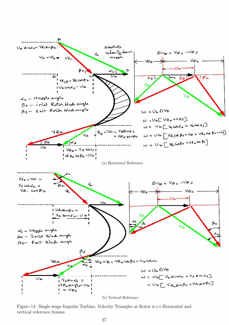
(a) Horizontal Reference

(b) Vertical Reference

Figure 14: Single stage Impulse Turbine, Velocity Triangles at Rotor w.r.t Horizontal andvertical reference frames

27

(a) Velocity Compounding (b) Pressure Compounding

Figure 15: Compounding of Impulse Turbines(Courtesy:-World Wide Web)

28