T H E A U S T R A L I A N N A T I O N A L U N I V E R S I T Y

Crawford School of Public Policy

TTPI Tax and Transfer Policy Institute

TTPI - Working Paper 7/2017 September 2017 Dr Chung Tran Research School of Economics, Australian National University Sebastian Wende Research School of Economics, Australian National University

Abstract

We quantify marginal excess burden, defined as the change in deadweight loss for an additional dollar of tax revenue, for different taxes. We use a dynamic general equilibrium, overlapping generations model featured with heterogeneous agents and a realistic structure of corporate finance and taxes. Our main results, based on an economy calibrated to Australian data, indicate that company taxes are more distorting than personal income and consumption taxes. Specifically, the marginal excess burden for the company income tax is 83 cents per dollar of tax revenue raised, compared to 34 cents and 24 cents for the personal income and consumption taxes, respectively. A broader analysis of more tax instruments confirm that the relatively larger excess burden of company taxes ultimately falls on households. Importantly, the marginal excess burden is distributed unevenly across skill types, generations and ages. This highlights political challenges when obtaining popular support for raising taxes. Hence, our analysis demonstrates that marginal excess burden can be a useful tool for evaluating both efficiency and distributional implications of a tax increase at the margin.

JEL Codes: E62, H21, H22, H24, H25.

Keywords: Taxation, fiscal distortion, overlapping generations, skill heterogeneity, corporate finance, deadweight loss, dynamic general equilibrium, welfare *. We thank Jenny Gordon, Patrick Jomini, Michael Kouparitsas, Bob Gregory, Maria Racionero, Rohan Alexander, Xavier Rimmer and participants at the 73rd Annual Congress of the International Institute of Public Finance, 2017 Asian Econometrics Society Meeting, 2016 Pension and Superannuation Workshop at the UNSW, and seminars at the Australian Productivity Commission, the Australian Parliamentary Budget Office, the Federal Treasury of Australia, Deloitte Access Economics, ANU Tax and Transfer Policy Institute and ANU Research School of Economics for many useful comments. All correspondence to Research School of Economics, the Australian National University, ACT 2601, Australia. Telephone: +61 6125 5638, Email: chung.tran@anu.edu.au. or sebastian.wende@anu.edu.au .

T H E A U S T R A L I A N N A T I O N A L U N I V E R S I T Y

Tax and Transfer Policy Institute

Crawford School of Public Policy

College of Asia and the Pacific

+61 2 6125 9318

tax.policy@anu.edu.au

The Australian National University

Canberra ACT 0200 Australia

www.anu.edu.au

The Tax and Transfer Policy Institute in the Crawford School of Public Policy has been established to

carry out research on tax and transfer policy, law and implementation for public benefit in Australia.

The research of TTPI focuses on key themes of economic prosperity, social equity and system

resilience. Responding to the need to adapt Australia’s tax and transfer system to meet contemporary

challenges, TTPI delivers policy-relevant research and seeks to inform public knowledge and debate

on tax and transfers in Australia, the region and the world. TTPI is committed to working with

governments, other academic scholars and institutions, business and the community.

The Crawford School of Public Policy is the Australian National University’s public policy school,

serving and influencing Australia, Asia and the Pacific through advanced policy research, graduate and

executive education, and policy impact.

1 Introduction

The projections for many OECD economies indicate that they are heading into eras of

�scal stress with rising public debt relative to GDP (e.g., see IMF (2010) and Cecchetti,

Mohanty and Zampolli (2010)). It is likely that governments will have to raise taxes to

�nance their existing spending commitments and to service increasing debt. A major

concern of raising taxes is the distortions they create. This leads to a number of questions:

How to assess welfare losses due to the adverse e�ects of tax increases on economic

activities? Which tax results in the lowest welfare cost per dollar of additional revenue?

And, who bears the welfare losses under di�erent taxes?

In this paper we address these important questions by quantifying marginal excess

burden (MEB), de�ned as the total welfare loss associated with one dollar of additional

tax revenue, for di�erent taxes in a dynamic general equilibrium, overlapping generations

model with heterogeneous agents. We primarily examine three di�erent taxes: company

income tax, personal income tax and consumption tax. In our extension, we analyse a

broader range of tax instruments imposed on households and �rms. Our main goal is

to better understand the deadweight loss of a tax increase at the point de�ned by the

current tax system, and the distribution of deadweight loss across households and over

time.

The marginal excess burden (MEB) analysis has been used extensively to evaluate

the e�ciency of the tax system in the public �nance literature (see Auerbach and Hines

(2002) for a review). In a static framework, the excess burden of taxation is commonly

measured by the area of the associated `Harberger triangle' (e.g., see Harberger (1964),

Hausman (1981) and Hines (1999)). Intuitively, the base of the Harberger triangle mea-

sures the amount by which economic behaviour changes as a result of price distortions

introduced by taxes. The MEB analysis computes the deadweight loss taken of a tax

increase at the point de�ned by the current tax legislation. It therefore can provide

local information; that is, welfare cost of a marginal tax increase. The MEB analysis is

related to the theory of optimal taxation. However, it di�ers both in its approach and

the underlying question it answers.

The theory of optimal taxation aims to characterize which tax system should be cho-

sen to maximize a social welfare function subject to a set of constraints. The optimal

taxation literature usually makes a normative choice on a social welfare function, which

aggregates the utility of individual households. The optimality of a particular tax sys-

tem depends on this choice of social welfare function (e.g., see Fehr and Kindermann

(2015)). The optimal tax analysis provides global information on the �best� tax system.

Conversely, MEB burden analysis measures the marginal welfare loss at current policy

settings. A measure of the distortion of current policy settings can act as motivator of

2

policy reform while optimal analysis provides insights of what a reform package should

look like. Understanding the local impacts of taxes at the current settings is more rele-

vant for decision making. The optimal tax analysis provides limited information on the

local impacts. The MEB analysis can �ll in this gap. Thus, the MEB and optimal tax

analyses provide complementing information.

We depart from the previous literature and formulate a dynamic general equilibrium,

overlapping generations (OLG) model with heterogenous agents. The model consists of

di�erent households, a perfectly competitive representative �rm and a government sector.

Households are of three skills types and enter the model at age 20 and potentially live

to 100. They make decisions on consumption, labour supply and saving to maximise

their lifetime utility. The households are forward looking and their decisions take into

account �ows of future after-tax incomes and the need for retirement savings. On the

production side, there is a representative �rm that produces output with its owned capital

and labour rented from the labour market. The �rm chooses investment to optimise its

market value taking into account future pro�ts and the structure of corporate �nance and

taxes. The �rm can use retained pro�ts or issue debt or equity to �nance its investment

plan. The �rm pays returns to debt and equity holders. The government collects taxes

to �nance two government spending programs: government consumption and transfers

to households.

We discipline the benchmark model to match data from Australia. Our model

matches key patterns of life-cycle behaviour and essential features of the Australian

macroeconomy in the 2010s. We �rst quantify the marginal excess burdens for three

major taxes in Australia: Company Income Tax (CIT), Personal Income Tax (PIT) and

Consumption Tax (CT).

Measuring marginal excess burden is more complex in a dynamic general equilibrium

framework since the Harberger triangle is not well de�ned. To get around this issue we

follow Judd (1987) and use Hicksian equivalent variation to measure the excess burden.

More speci�cally, we compute it in two steps. We �rst compute the equivalent variation

for all households over the transition path and in the new steady state. These speci�c

excess burdens are a measure of welfare costs that individual households bear after raising

taxes. Next, we construct a metric of the aggregate marginal excess burden in terms of

the net present value of the excess welfare losses by all households normalised by dividing

by the net present value of the change in net revenue. We call this metric the aggregate

marginal excess burden (AMEB). In the baseline scenarios, only one tax rate is changed

and the government budget is balanced by returning the additional revenue back to

households via uniform lump sum transfers.1 Technically, the AMEB measures the total

1It is important to note that the MEB analysis conducted here uses scenarios that each raise netrevenue by the equivalent of one dollar per period in net present value terms. As the revenue changeis uniform the impacts are directly comparable. Only one tax change is varied in each scenario which

3

distortion of the particular tax relative to a lump sum tax at the point de�ned by the

current tax system. Moreover, in our heterogenous agents model it is straightforward to

compute disaggregated MEB by household characteristics.

Our main results are as follows. First, we �nd that the marginal excess burden for the

company income tax is 83 cents per dollar of tax revenue collected, which is much higher

than 34 cents and 24 cents found for the personal income tax and the consumption tax,

respectively. This �nding indicates that the company income tax results in the largest

aggregate deadweight loss. The main reason is that foreign capital is highly mobile and

therefore responsive to the company tax in a small open economy model. An increase in

the company income tax discourages investment and subsequently decreases the capital

stock, productivity and wages.

We show that the welfare losses are not evenly distributed as the marginal excess

burden varies signi�cantly across skill types, ages and generations. We �nd that over-

65s, on average, are the biggest losers from a company tax increase. They lose less from

increases in the personal income tax or the consumption tax. Lower-income households

would be, on average, largely una�ected by a company tax hike. This occurs as the model

assumes any extra revenue generated is re-distributed evenly via the transfer system to

balance the budget, the loss of income from lower wages is o�set by higher transfer.

Further, low income households would be 32 cents better o� under an income tax rise

and 16 cents better o� if the consumption tax increased again due to the additional

transfers.

Moreover, we consider other tax instruments, including investment tax credits (ITC),

depreciation deductions (DD), personal labour income tax (PLT) and personal asset

income tax (PAT). We �nd that the taxes which are broadly considered as falling on

capital result in higher marginal excess burden than the taxes on labor and consumption

in our framework. The overall ranking is that reducing investment tax credits results

in the highest marginal excess burden, while raising consumption tax causes the lowest

marginal excess burden. Interestingly, even though a reduction in the investment tax

credits has the highest welfare cost at the aggregate level the households alive at the

time of the policy change are better o�.

Finally, we consider di�erent model speci�cations and calibration assumptions, in-

cluding the openness of the economy, alternative methods to allocate additional tax

revenue, the foreign ownership share, the role of �xed factors, franking credits, capital

adjustment speed, economic growth, the intertemporal elasticity of substitution and the

elasticity of labor supply. We �nd that our main results are fairly robust.

Thus, we demonstrate that the marginal excess burden is an e�ective index for com-

isolates the impacts of individual taxes. If the revenue increase were used to fund a cut in anothernon-lump sum tax then the impacts would be due to two changes and disentangling the e�ects wouldbe more di�cult.

4

paring the distortion of di�erent taxes at the margin. It can be used to facilitate the

comparison of a large number of taxes both in terms of aggregate distortions and dis-

tributional impacts. We show that both the aggregate marginal excess burden and the

group-speci�c marginal excess burden are useful for understanding the e�ciency and

distributional e�ects of tax increases. Our result has implications for evaluating alter-

native designs of a tax reform plan. It indeed provides essential information for public

policy debates around the `best' option to raise tax revenue. Furthermore, a better un-

derstanding of the distribution of marginal excess burdens allows policy makers to put

together a more feasible package of tax increases required to close �scal gaps. Indeed,

the marginal excess burden approach is particularly suited to improve communication

between academics and policy makers and to bridge the gap between academic research

and policy making.

Related literature

Our work is connected to several branches of the macroeconomic/public �nance litera-

ture. First, our paper extends the large literature analysing the excess burden of taxation.

The early work studies excess burden in a static framework (e.g., see Feldstein (1978),

King (1983), Feldstein (1995), Fullerton and Henderson (1989), and Hines (1999)). Note

that, these micro and empirical estimates of excess burden do not take into account

dynamic changes in the labour and capital markets and general equilibrium price adjust-

ments in response to tax increases. Auerbach, Kotliko� and Skinner (1983), Chamley

(1981) and Ballard, Shoven and Whalley (1985) extend the excess burden approach to

general equilibrium frameworks. They concentrate on approximating the total excess

burden of large tax changes. Judd (1985a) and Judd (1987) analyses the marginal excess

burden of taxation using a representative agent model. In particular, Ballard, Shoven

and Whalley (1985) �nd MEB estimates in the range of 18 to 46 cents for industry level

capital tax and a range of 12 to 23 cents for industry level labour taxes. Judd (1985b)

�nds a MEB of 12 cents for labour income tax, 98 cents for a tax on dividends and

interest payments, and −16 dollars for an investment tax credit. We deviate from the

previous studies and formulate a dynamic general equilibrium with heterogenous agents

and a realistic structure of corporate �nance and taxes. We also take into account both

long-run steady state e�ects and dynamic e�ects along the transition path. As a result,

we �nd our MEB estimates are relatively larger. More importantly, our new modelling

approach allows us to map out the distribution of marginal excess burdens across house-

holds. We show that deadweight losses of raising one additional revenue are heterogenous

across households and over time.

Our work links the literature on the marginal excess burdens of taxes to the literature

on the dynamic e�ects of taxes. Since Auerbach and Kotliko� (1987) there is a large

5

literature analysing aggregate and welfare e�ects of various tax schemes, using a large

scale overlapping generations (OLG) models. Auerbach and Kotliko� (1987) show that

while replacing income tax with wage tax reduces e�ciency, replacing income tax with

consumption tax increases e�ciency. Imrohoroglu (1998) �nds that a positive capital

income tax rate maximizes steady state welfare. In a similar environment, Ventura

(1999) shows that the elimination of capital income taxation positively a�ects capital

accumulation. Fuster, Imrohoroglu and Imrohoroglu (2007) study the e�ects of di�erent

revenue-neutral tax reforms that eliminate capital income taxation and show that the

majority of the population alive at the time of the reform bene�t from it in the dynastic

framework. Conesa, Kitao and Krueger (2009) �nd that the optimal capital income

tax rate is strictly positive at 36 percent in an overlapping generations economy with

incomplete markets and heterogeneous agents. The policy experiments in this literature

involves raising some taxes while lowering others to maintain a balanced government

budget. As such changes in welfare are due to multiple tax changes and disentangling the

impacts of each taxes is more di�cult. We follow a similar OLG modelling approach and

explicitly model corporate tax policy and how a �rm optimally �nances its investment

plan. Di�erently, we quantify the economic cost of only one tax change at the margin.

We demonstrate that understanding the impacts of tax increases at current state of

tax policy settings, especially the distributional consequences, is important for policy

making.

Our paper is related to the literature on dynamic scoring of tax cuts. Mankiw and

Weinzierl (2006) studies the extent to which a tax cut pays for itself through increased

activity. Leeper and Yang (2008) emphasize the role of tax �nancing instruments when

calculating the tax scoring. That literature is motivated by President Bush's early 2000s

tax cuts in the United States. In the dynamic scoring literature, the dynamic revenue

estimate takes the behavioural responses and general equilibrium adjustments into ac-

count. Dynamic scoring of a tax rate computes the derivative of the dynamic tax revenue

taken at the point de�ned by the current tax legislation. The MEB approach is analo-

gous to the dynamic scoring approach as it measures the e�ects at the margin. However,

it focuses more on the economic cost of raising taxes. In our analysis, we can compare

the static revenue increase required to raise an additional net dollar once the dynamic

responses of agents and general equilibrium channels are taken into account. Further-

more, we go beyond revenue implication and map out marginal welfare costs for di�erent

households at the point de�ned by the current tax system.

Our paper contributes to the analysis of the Australian tax system. Several policy

papers including Cao et al. (2015) apply the marginal excess burden approach to evaluate

the e�ciency cost of tax reforms in Australia, using static multi-industry computable

general equilibrium (CGE) models. However, the CGE modelling approach lacks many

6

important features as it abstracts from microfoundations of inter-temporal behaviour.

These CGE models exclude dynamics of investment and capital accumulation and fail

to account for the transition dynamics. There is a growing literature using overlapping

generations (OLG) models to analyse the dynamic e�ects of the Australian tax and

transfer policies (e.g. see Tran and Woodland (2014), Kudrna, Tran and Woodland

(2015) and Kudrna, Tran and Woodland (Forthcoming)). However, these papers do not

assess the marginal distortions of taxes in Australia, which is the focus of our paper.

The paper is structured as follows. Section 2 describes the model. Section 3 provides

details on the calibration of our model to the Australian economy and its �t to the

data. In Section 4 we present the quantitative analysis. Section 5 includes extensions

and sensitivity analysis. Section 6 concludes. The Appendix contains additional tables

and �gures. The derivation of the key equations and description of the computational

methods is contained in an online technical appendix.

2 Model

The model is a discrete time dynamic general equilibrium model, which consists of over-

lapping households, a perfectly competitive representative �rm, foreign investors with

perfectly capital mobility and a government with full commitment technology.

2.1 Demographics

The model is populated by households of di�erent ages between 20 and 100, j ∈ J =

[20, . . . , 100], and three di�erent skill types i ∈ I =[1, 2, 3].

In each period a continuum of households aged 20 enters the model and live to at most

age 100 . They face a stochastic probability of death every period, spj the age-dependent

survival probability at age j. The unconditional probability of surviving from age 20 to

age j, is given by Sj =∏j

s=21 sps. The size of a new cohort entering the economy and

the overall population both grow at the rate gn. Mt,j,i denotes the size of the cohort

of skill type i in age j at time t, which evolves according to Mt+1,j+1,i = spj+1Mt,j,i =

Mt,j+1,i(1 + gn).

2.2 Household

Preferences. Households maximise expected lifetime utility which is the sum of current

and discounted future intra-temporal utility adjusted for the chance of death

Ut,j,i =100∑j′=j

Sjβ̂j′−ju (Ct+j′−j,j′,i, lt+j′−j,j′,i)

7

where β̂ is the time discount factor and Sj is the unconditional probability of survival.

Households have identical intra-temporal preferences over consumption, Ct,j,i ≥ 0, and

leisure, 0 ≤ lt,j,i ≤ 1. The intra-temporal utility is assumed to have the form

u (Ct,j,i, lt,j,i) =

(Cγt,j,il

1−γt,j,i

)1−σ

1− σ,

where σ is a parameter governing inter-temporal elasticity of substitution and γ is the

consumption share of utility.

Endowments. Households are di�erent by skill type and age in our model. New

households enter the model with a speci�c income type that determines their labour

productivity over their life cycle. Labour e�ciency unit, denoted by ej,i, is type and age

dependent but time-invariant. In each period, households are endowed with one unit

of time that can be allocated over labour market and leisure activities. As such, each

household's before-tax labour income is given byWt (1− lt,j,i) ej,i whereWt is the market

wage rate in period t.

Household problem. Households begin with zero assets, At,20,i = 0, and choose

consumption, labour supply and asset holdings to maximise their utility over their life-

time. In our inter-temporal setting, households are able to save to smooth consumption

over the life cycle by buying/selling asset holdings, At,j,i, which yields a dividend rat , at

a market price pat . Households are restricted to a no borrowing constraint at all times,

At,j,i ≥ 0.

There are several sources of income. Households receive incomes from supplying la-

bor and holding assets, Wt(1− lt,j,i)ej,i + ratAt,j,i. Households receive transfers from the

government to o�set the company tax paid by the �rm through a dividend imputation

system. The amount of franking credits is given by rFCt At,j,i, where rFCt is the franking

credit per asset unit. In addition, households receive lump-sum transfer from the gov-

ernment Tt,j,i and accidental bequests, BQt,i.2 Household are required to pay personal

income tax at the rate of τ p. A typical household's taxable income includes labor, asset

and franking credit incomes. The household's disposable income is given by

Υt,j,i = (1− τ pt )[Wt(1− lt,j,i)ej,i + ratAt,j,i + rFCt At,j,i

]+ patAt,j,i + Tt,j,i +BQt,i.

The household's utility maximisation problem can be written in terms of a dynamic

programming problem as

Vj(At,j,i) = max{Ct,j,i,lt,j,i,At+1,j+1,i}

{u (Ct,j,i, lt,j,i) + β̂spj+1Vj+1 (At+1,j+1,i)

}(1)

2We abstract from any intended bequests and all inter-generational transfers are accidental. House-holds face uncertain death and therefore may die with positive asset holdings. The assets of the deceasedare redistributed equally to all surviving households of the same type.

8

subject to the household's budget constraint patAt+1,j+1,i+(1+τ ct )Ct,j,i = Υt,j,i, the credit

constraint, At+1,j+1,i ≥ 0, and the positivity of leisure and consumption Ct,j,i > 0 and

1 ≥ lt,j,i > 0.3

2.3 Firm

The production sector consists of one representative �rm which owns capital and the

�xed factor and chooses investment, dividends, debt and equity and to maximise its cum

dividend share price.

Technology. Output is produced by combining capital, Kt, e�ective labour, Nt, and

a �xed factor, Zt, in a constant returns to scale Cobb-Douglas production,

Yt = Ft (Kt, Nt) = ZtKαkt (ΛtNt)

αn .

Capital's share of output is αk and αn is labour's share. Λt is the labour augmenting

level of technology and grows at the constant rate gΛ.4

Capital is accumulated according to the law of motion

Kt+1 = (1− δ)Kt + It, (2)

where It is investment and δ is the depreciation rate.

Investment is subject to a quadratic capital adjustments cost with the total cost of

investment given by

It + 0.5ψ

(ItKt

)2

Kt.

Corporate �nance. The �rm is owned by equity holders. There are two channels

to �nance the �rm's investment plan: internal �nance by retained incomes and external

�nance by issuing new equity and debt. For simplicity, we make two assumptions: (i)

equity is set equal to capital, Θt = Kt, which sets equity issuance equal to net investment;

and (ii) debt is set at a constant fraction of real capital as in Poterba and Summers

(1983), so that the level of debt is given by Bft = ξKt, where ξ is a �xed debt to real

capital ratio.5 This debt to capital assumption is used to cap debt holdings in the model.

As debt receives preferential tax treatment the �rm would be completely debt �nanced

3Technically, the e�ective rate of return on holding assets is r̃t = rat + rFCt .4In our setting, output per capita grows by labour augmenting productivity in steady state. As such

we de�ne the e�ective �xed factor as Zt = (ΛZt Z̄)1−αk−αn where ΛZt is the �xed factor augmenting levelof technology and Z̄ is the �xed factor. We assume �xed factor augmenting productivity grows by thecompound sum of labour augmenting productivity and population growth, gZ = gΛ + gn + gΛgn = gΛn

implying it grows at the same rate as steady state output.5The price of capital when calculating the value of debt is one.

9

if there is no cap.6

Company tax and deductions. We model some key features of corporate tax

structure. The �rm pays company income tax (CIT) on its income which is revenue

minus wages, τ k (Yt − wtNt). The �rm can also deduct from its taxable income a fraction

of its interest payments, investment and capital depreciation. The value of the tax

deductions for interest paid is given by χξrft Bft , where r

f is an adjusted interest rate and

χξ is a deductible fraction of its interest payment.7 The value of investment tax credits

(expensing deductions) is given by χIIt, where χI is a deductible fraction of its investment

cost. The value of depreciation deductions is equal to χδδKt, where χδ is a deductible

fraction of depreciation cost. The total deduction is given by(χξrft B

ft + χIIt + χδδKt

).

Firm problem. The �rm maximises its own value which is given by its cum dividend

price multiplied by the number of shares Vt = p∗tΘt = (pt + dt)Θt. The value of the �rm

can be expressed in terms of dividend payments and new equity issuances as

Vt0 =∞∑t=t0

dtΘt + pt(Θt+1 −Θt)∏ts=t0

(1 + rs). (3)

The �rm's problem is to choose a sequence of{It, dt, B

ft ,Θt+1

}∞t=t0

to maximize its

market value and subject to its budget constraint

It + 0.5ψI2t

Kt

+ dtΘt + rtBft = (1− τ kt ) [Ft (Kt, Nt)−WtNt] + pkt (Θt+1 −Θt)

+ (Bft+1 −B

ft ) + τ kt

(χξrft B

ft + χIIt + χδδKt

), (4)

taking account wage rate, interest rate and the company tax policy as given. The �rm's

problem is also subject to the capital accumulation equation (2). The stock of debt

and equity are further subject to the simplifying assumptions discussed in the corporate

�nance section.

2.4 Government

The government collects revenue from taxing household and �rm incomes and household

consumption to �nance government purchases and transfers.

Taxes. The government raises revenues from company income tax, personal income

tax and consumption tax. The �rm pays company income tax on its gross income with

6The equity to capital assumption is a simplifying assumption as the �rm is indi�erent betweenpaying returns as capital gains or as dividends. This stems from Miller and Modigliani (1961) and ourassumption that the marginal foreign investor pays neither dividend taxes nor capital gains taxes, or ifthey do that the rates are equal.

7The interest rate used for tax deductions, rf , takes into account that �rms are able to deductnominal interest payments. See the technical appendix for further details.

10

deductions. The full range of deductions is described in the �rm section (??). Total

revenue from the company income tax is given by

TAXkt = τ kt

[Ft (Kt, Nt)−WtNt − χδδKt − χξrft ξKt − χIIt

].

A dividend imputation system to compensates resident households for the company

income tax paid by �rms. The value of the franking credit per share is computed by

rFCt = χFC TAXk

Θt, where χFC is the share of company income tax paid that �rms distribute

as franking credits.

Households pay labour and asset incomes are taxed at the rates of τ p. However,

they use franking credits against the value of their asset income, rFCt At,j,i. The sum of

personal income taxes paid by all households is given by

TAXpt =

∑j∈J

∑i∈I

Mt,j,i

{τ pt[(Wt(1− lt,j,i)ej,i +

(rat + rFCt

)At,j,i

)]− rFCt At,j,i

}.

The government revenue from consumption tax, TAXct , is given by

TAXct = τ ctCt,

where τ ct is consumption tax rate and Ct is total private consumption.

Hence, the total tax revenue is a sum of three tax revenues: TAXt = TAXpt +TAXk

t +

TAXct .

Expenditures. The government has two spending programs: the purchase of goods

for government consumption, Gt, and government transfers, Tt. Government consump-

tion and transfers grow in line with productivity and population. Government transfers

encompass pension payments and other social security transfers. The total amount of

government transfers, Tt, is the sum of transfers to all households

Tt =∑j∈J

∑i∈I

Mt,j,iTt,j,i,

where Mt,j,i is the measure of age j and type i households at time t and Tt,j,i is the

amount of transfers received by individual households which grow in line with labour

augmenting productivity.

Budget balancing rule. How the government balances its budget depends on the

scenario. In the baseline the government's budget is balanced in every year and the

government starts with zero debt. When the government borrows or lends the evolution

of government bonds, BGt , is given by

BGt+1 = TAXt −Gt − Tt − (1 + rt)B

Gt . (5)

11

We assume that the government can borrow and lend at the international interest rate

and that all government debt is held by foreigners. In this case the government's budget

is balanced by ensuring the net present value of revenue equals that of spending.

∞∑t=0

TAXt∏ts=0(1 + rs)

=∞∑t=0

Gt + Tt∏ts=0(1 + rs)

. (6)

2.5 Markets

The economy is small and open with perfect capital and goods mobility. The labour

market is assumed to be perfectly competitive with the wage equal to the marginal

product of labour. Labour is assumed to be internationally immobile implying workers

can not migrate in response to economic conditions.

In the domestic �nancial market, there exists an asset combining agency that com-

bines equity and debt issued by the �rm into a single asset which is sold to both residents

and foreigners. One unit of the combined asset is de�ned as one unit of equity plus the

proportional share, ξ, of debt. As such the stock of assets equals the stock of equity

which equals the capital stock and also the stock of �rm bonds divided by the debt

�nancing ratio

At = Θt = Kt = Bft /ξ. (7)

The price of the combined asset, pat , is the price of equity plus the share of debt used in

funding the �rm and is given by pat = pkt + ξ. The return on the combined asset is given

by the return on debt plus the return on equity and is given by rat = ξrt + dt.

The domestic capital market is fully integrated into the world capital market. As such,

foreigners are the marginal investors and the domestic interest rate, rt, is exogenous and

equal to the world interest rate, rt = r. The domestic �rm therefore uses the international

interest rate in its maximisation problem. As such the rate of return on domestic assets

must equal the international interest rate

rat+1 + pat+1 − patpat

= rt = r. (8)

Foreign goods and domestic goods are perfect substitutes hence only net exports are

tracked in the model. Net exports (NXt) are determined by the balance of payments

and are given by

NXt = ratAfort − pat (A

fort+1 − A

fort ) + rtD

Gt − (DG

t+1 −DGt ), (9)

where Afort is the total assets held by foreigners.

12

2.6 Competitive equilibrium

The solution to the model is given by prices and quantities that are consistent with the

solutions to the households' and �rm's problems, the government's budget constraint

and foreigners' required rate of return.

For a given model calibration an equilibrium is de�ned by a set of household decisions

{Ct,j,i, lt,j,i, At+1,j+1,i}t∈T,j∈J,i∈I; a set of �rm decisions including labour demand, capital

stock, investment, equity and debt {Nt, Kt+1, It,Θt+1, Bft , }t∈T; a set of relative prices for

wages, assets and returns on assets {Wt, pat , r

at , r

FCt }t∈T; accidental bequests {BQt,i}t∈T;

government policy settings {τ ct , τpt , τ

kt , χ

ξ, χI , χδ, Gt, Tt}t∈T; and foreign assets and net

exports {Afort , NXt}t∈T such that the following hold:

1. the choice of leisure, asset accumulation and consumption are consistent with the

solutions to household's problem given in equation (1),

2. the investment, capital stock, dividends, �rm debt and the stock of equity are

consistent with the solution �rm's problem given in equation (3),

3. the return to assets and the price of assets are consistent with return required by

foreign investors as given in equation (8),

4. the government's budget balances as given in equation (6),

5. the sum of individual consumption, labour supply, and asset holdings equals ag-

gregate consumption, labour demand, and aggregate domestically owned assets,

Ct =∑j∈J

∑i∈I

Mt,j,iCt,j,i,

Nt =∑j∈J

∑i∈I

Mt,j,i(1− lt,j,i)ej,i,

Adomt =∑j∈J

∑i∈I

Mt,j,iAt,j,i

6. the capital stock equals the total stock of assets as in equation (7), with total assets

equal to the sum of domestic assets plus foreign owned assets

At = Adomt + Afort , (10)

7. the aggregate resource constraint holds, with total production equalling the total

use of output as given below

Kαkt (ΛtNt)

αn(ΛZt Z)1−αk−αn = Ct +Gt + It + 0.5ψ

(ItKt

)2

Kt +NXt, (11)

13

where net exports are given by equation (9) with government bonds evolving ac-

cording to equation (5),

8. bequests are equal to the deceased's assets, including returns, evenly distributed

amongst the remaining agents of that type as given by

BQt,j,i =

∑j∈J (Mt−1,j,i −Mt,j+1,i) (pat + rat )At,j+1,i∑

j∈JMt,j,i

. (12)

3 Calibration

This section describes how parameters of the model are calibrated. The majority of

the parameters are calibrated so that the model matches Australian macroeconomic

aggregates. Other parameters are calibrated so that household variables match micro-

economic data from the Household, Income and Labour Dynamics in Australia (HILDA)

survey or taken from the literature.8 The frequency of the model is annual and the unit of

the model is an individual who represents a household. As a basis of the calibration, we

�rst compute a benchmark steady state economy that approximates the economy of 2010.

We summarize these external parameters in Table 4. Internally selected parameters to

match a given set of targets from Australian data are presented in table 5.

3.1 Demographics

The population dynamics are calibrated to match the Australian Bureau of Statistic's

(ABS) release 3222.0 Population Projections. The population dynamics are set to match

the evolution of the cohort of persons aged 20 in 2013-14. De�ning Pop20,2014 to be

the population of persons aged 20 at 1 June 2014 the conditional survival probability is

calculated as sp∗21 = Pop21,2015/Pop20,2014. Due to positive net migration the projected

size of some age cohorts increases but we set the conditional survival probability to a

maximum value of one.

The three skill levels are de�ned by three education levels. Let Pi denote the shareof the population with skill type i. The share of the population with skill type i at age

j is given by mj,i = Pi Sj(1+gn)j−20∑100j=20 Sj(1+gn)j−20 .

The growth in the population is also calibrated to the ABS's release 3222.0 Population

Projections. Growth in the population of persons aged 20 and over is projected to average

8This paper uses unit record data from the Household, Income and Labour Dynamics in Australia(HILDA) Survey. The HILDA Project was initiated and is funded by the Australian Government De-partment of Families, Housing, Community Services and Indigenous A�airs (FaHCSIA) and is managedby the Melbourne Institute of Applied Economic and Social Research (Melbourne Institute). The �nd-ings and views reported in this paper, however, are those of the author and should not be attributed toeither FaHCSIA or the Melbourne Institute.

14

1.7 per cent from now to 2050 and we use this value for gn.

3.2 Household

The consumption share of utility γ is set to 0.25 so that the share of hours spent at work

in the model matches HILDA data. The inter-temporal elasticity 1/σ is set to 0.4 as in

Kudrna, Tran and Woodland (2015).

The labour e�ciency endowments are estimated from HILDA data. The skill type

levels are matched to education levels as reported in HILDA. The shares from in HILDA

give the populations shares of the skill types in our calibration.

3.3 Firm

The labour share of output, αn, is set at 0.59, so that the labour share of output matches

the average ratio of gross operating surplus to compensation of employees from 1990 to

2014 as in ABS 5204.006.9 Further, the capital share of output, αk, is set at 0.39, so that

the �xed factors share of output matches the 2 per cent contribution of non-residential

land to GDP as in Cao et al. (2015). The depreciation rate, δ, is set at 5.6 per cent

to match the investment to capital stock ratio in the data. We use the steady state

relationship δ + n + g + n ∗ g = I/K and target the average ratio of gross �xed capital

formation to the end of year net capital stock from 1990 to 2014, in both cases excluding

dwelling.

The capital adjustment cost ψ is set to 3.33 to target the steady state q-ratio of 1.14

from Oliner, Rudebusch and Sichel (1995). Labour augmenting productivity growth, gΛ,

is set to 1.7 per cent to match growth in per capita GDP from 1990 to 2014.

We follow Cao et al. (2015) to assume that the �rm issues franking credits for 36.8

per cent of the tax they pay meaning χFC = 0.368. The �rm is 24 per cent debt funded

and is able to deduct 100 per cent of its interest payments, χξ = 1.0. The �rm receives

investment tax credits for 5 per cent of its investment, χI = 0.05, and is able to claim

the remaining 95 per cent as depreciation deductions χd = 0.95.

3.4 Government

Tax rates are set to match revenue to GDP ratios as from ABS 5506. The company

income tax (CIT) rate τ k is set to 33.0 per cent to match the CIT to GDP ratio of 5.4

per cent. The personal income tax (PIT) rate τ p is set to 16.1 per cent to match PIT to

9We assume that the capital share of gross mixed income matches the capital share in gross operatingsurplus and compensation of employees.

15

GDP ratio of 10.4 percent. The consumption tax (CT) rate τ c is set to 6.2 per cent to

achieve the consumption tax revenue to GDP ratio of 3.6 per cent.

Transfers are calibrated based on data from Australian Bureau of Statistics: ABS

5204.030 and ABS 6537 where aggregate pensions average 2.7 per cent of GDP from

1990 to 2014. Other social assistance payments excluding pensions average 5.2 percent

of GDP. Beyond matching the social transfers to GDP an attempt is made the match

the income quintiles in ABS 6537 in the model.

Government purchases of goods are set to 11.5 per cent of GDP, so that the budget

balances in the baseline.

3.5 Markets

The world interest rate r is set to target the capital stock to GDP ratio. The capital

stock to GDP target is calculated from 1990 to 2014.10 The target capital output ratio

equal to 3.1 implies a world interest rate, r, equal to 3.8 per cent in the model.

The discount rate β is used to target the domestic ownership of the capital stock.

The discount rate determines agent's time preference and therefore their savings and

asset accumulation. As there is no concise closed form solution for asset accumulation

and β is solved iteratively. In the model β equals 0.978 giving net foreign ownership of

17 per cent in line with the average net international investment position relative to the

total capital stock from 1990 to 2015.

3.6 Benchmark model

Our benchmark model matches the macroeconomic data. In addition, it can replicate

the life cycle patterns of Australian households. Figure 1 depicts the asset holdings and

labor supply over the life cycle. Figure 1 presents the asset accumulation in the model,

compared to that in HILDA. In the model households save for retirement but are bound

by the borrowing constraint in the early part of their lives when their labour productivity

is lower. Figure 1(b) shows the broad similarities between the labour supply pro�les in

the model and in the HILDA data.

10The relationship between the interest rate and the capital output ratio is given in the technicalappendix.

16

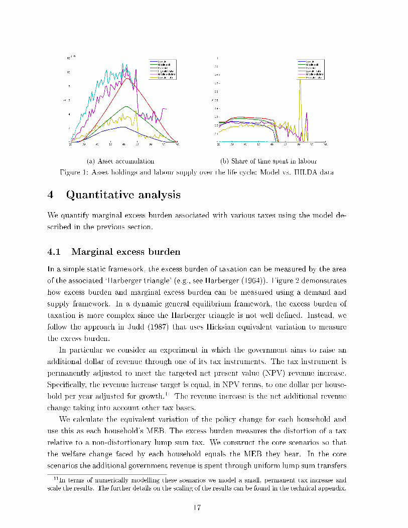
(a) Asset accumulation (b) Share of time spent in labour

Figure 1: Asset holdings and labour supply over the life cycle: Model vs. HILDA data

4 Quantitative analysis

We quantify marginal excess burden associated with various taxes using the model de-

scribed in the previous section.

4.1 Marginal excess burden

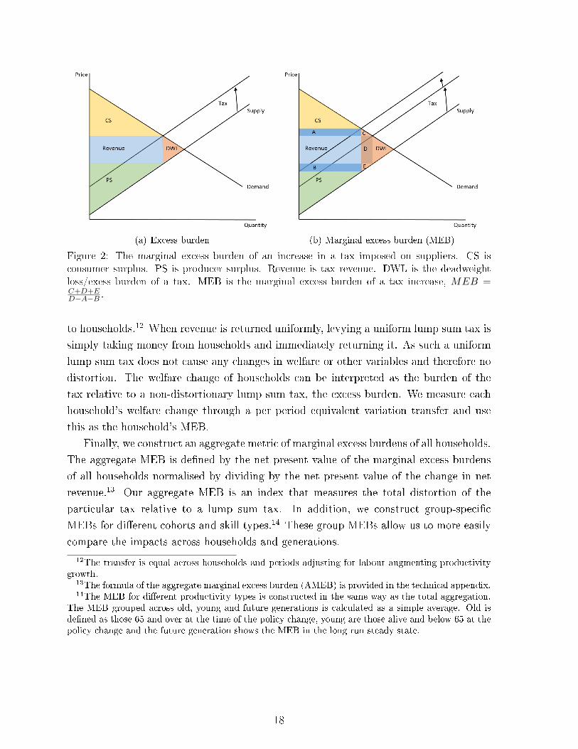
In a simple static framework, the excess burden of taxation can be measured by the area

of the associated `Harberger triangle' (e.g., see Harberger (1964)). Figure 2 demonstrates

how excess burden and marginal excess burden can be measured using a demand and

supply framework. In a dynamic general equilibrium framework, the excess burden of

taxation is more complex since the Harberger triangle is not well de�ned. Instead, we

follow the approach in Judd (1987) that uses Hicksian equivalent variation to measure

the excess burden.

In particular we consider an experiment in which the government aims to raise an

additional dollar of revenue through one of its tax instruments. The tax instrument is

permanently adjusted to meet the targeted net present value (NPV) revenue increase.

Speci�cally, the revenue increase target is equal, in NPV terms, to one dollar per house-

hold per year adjusted for growth.11 The revenue increase is the net additional revenue

change taking into account other tax bases.

We calculate the equivalent variation of the policy change for each household and

use this as each household's MEB. The excess burden measures the distortion of a tax

relative to a non-distortionary lump sum tax. We construct the core scenarios so that

the welfare change faced by each household equals the MEB they bear. In the core

scenarios the additional government revenue is spent through uniform lump sum transfers

11In terms of numerically modelling these scenarios we model a small, permanent tax increase andscale the results. The further details on the scaling of the results can be found in the technical appendix.

17

(a) Excess burden (b) Marginal excess burden (MEB)

Figure 2: The marginal excess burden of an increase in a tax imposed on suppliers. CS isconsumer surplus. PS is producer surplus. Revenue is tax revenue. DWL is the deadweightloss/exess burden of a tax. MEB is the marginal excess burden of a tax increase, MEB =C+D+ED−A−B .

to households.12 When revenue is returned uniformly, levying a uniform lump sum tax is

simply taking money from households and immediately returning it. As such a uniform

lump sum tax does not cause any changes in welfare or other variables and therefore no

distortion. The welfare change of households can be interpreted as the burden of the

tax relative to a non-distortionary lump sum tax, the excess burden. We measure each

household's welfare change through a per period equivalent variation transfer and use

this as the household's MEB.

Finally, we construct an aggregate metric of marginal excess burdens of all households.

The aggregate MEB is de�ned by the net present value of the marginal excess burdens

of all households normalised by dividing by the net present value of the change in net

revenue.13 Our aggregate MEB is an index that measures the total distortion of the

particular tax relative to a lump sum tax. In addition, we construct group-speci�c

MEBs for di�erent cohorts and skill types.14 These group MEBs allow us to more easily

compare the impacts across households and generations.

12The transfer is equal across households and periods adjusting for labour augmenting productivitygrowth.

13The formula of the aggregate marginal excess burden (AMEB) is provided in the technical appendix.14The MEB for di�erent productivity types is constructed in the same way as the total aggregation.

The MEB grouped across old, young and future generations is calculated as a simple average. Old isde�ned as those 65 and over at the time of the policy change, young are those alive and below 65 at thepolicy change and the future generation shows the MEB in the long run steady state.

18

4.2 Three main taxes

In this section, we quantify marginal excess burdens for three main taxes: company

income tax (CIT), personal/individual income tax (PIT) and consumption tax (CT).

Table 1 presents the marginal excess burdens (MEB) for di�erent taxes by di�erent

groups of households.15

CIT PIT CTAggregate $0.83 $0.34 $0.24Old: 65+ $1.32 -$0.64 $0.01Young: 20 to 64 $0.54 $0.09 $0.23Future: -100 $0.96 $0.44 $0.25Type 1: low income -$0.02 -$0.32 -$0.16Type 2: medium income $0.73 $0.27 $0.18Type 3: high income $1.75 $1.04 $0.70

Table 1: Marginal excess burdens (MEB) of raising extra revenue from the company

income tax (CIT), the personal income tax (PIT) and the consumption tax (CT).

Our main results indicate that raising the company income tax is more distorting

than raising the personal income tax and the consumption tax. As shown in the �rst

row of Table 1, the aggregate MEB for the company income tax is 83 cents per dollar of

tax revenue raised, compared to 34 cents and 24 cents for the personal income tax and the

consumption tax, respectively. Our MEB estimates are relatively larger than estimates

from previous studies using more simpli�ed models abstracted from lifecycle behaviour

and transition dynamics. Ballard, Shoven and Whalley (1985) �nd MEB estimates in

the range of 18 to 46 cents for industry level capital tax and a range of 12 to 23 cents

for industry level labour taxes. Judd (1985b) �nds a MEB of 12 cents for labour income

tax. It is important to note that we use a more comprehensive model in which we fully

account for dynamic general equilibrium e�ects in steady state and along transition path.

The company income tax is the least preferred tax as it results in highest MEB at the

aggregate level. However, when the welfare impacts are further disaggregated this does

not hold for all households as presented in rows from 2 to 6 in Table 1. There is signi�cant

variation in the MEB across generations and income types. The marginal excess burden

for each tax is unevenly distributed. In particular, old households are the biggest losers

from a company tax increase, but su�er less from increases in the personal income tax or

the consumption tax. Lower-income households would be largely una�ected by tax hikes.

This occurs as the model assumes any extra revenue generated is re-distributed evenly

15The results presented are normalised for population and productivity growth with the populationmeasure normalised to one. In this setting one dollar per household equals one dollar in total. Changesin aggregate variables, such as GDP and the capital stock, can be thought of as the change per dollarof net revenue. At the same time changes in households variables, such as welfare, can be thought of asthe change per dollar of revenue per household.

19

via the transfer system to balance the budget, the loss of income from lower wages is

o�set by higher transfer. Low-income households indeed would be 32 cents and 16 cents

better o� under income tax and consumption tax increases, respectively. Conversely,

high-income households would be worse o� as they bear most MEB.

We next examine each individual tax and analyse the underlying mechanisms through

which it distorts economic activity and welfare.

Company income tax (CIT)

Figure 3 displays the dynamic e�ects of the company income tax (CIT) increase on four

key variables: excess burden, tax revenue, capital stock and labour income. Figure 6 in

Appendix presents further information on other variables including interest and dividend

payments, after tax asset incomes, labor supply and asset holdings over the life cycles.

The CIT increase distorts the �rm's incentive to invest. Higher company income tax

rate lowers dividends, which subsequently lowers the value of capital and investment,

as seen in Panel 3 of Figure 3. As the capital stock decreases the marginal product of

capital increases ensuring dividends meet the foreign investors required rate of return.

However, resident's returns are higher in the long run as they receive franking credits

which increase in value. A lower capital stock decreases the marginal product of labour

and therefore wages.

Household's responses to these changes can be understood in terms of both income

and substitution e�ects of lower wages, higher transfers, reduced asset prices and chang-

ing rates of return. Panel 4 of Figure 3 shows labour supply decreasing as the substitution

e�ect from lower wages is larger than the accompanying income e�ect, especially given

the o�setting impact of higher transfers. Households also shift the timing of labour

supply forward across their life in response to higher asset returns created for residents.

This is matched by increased domestic saving.

The magnitude of the aggregate welfare loss per dollar of revenue is largely explained

by the fall in wages relative to the change in revenue. Increasing company income tax to

raise one dollar of net revenue reduces long run labour income by $3.44 of which $2.02 is

due to the decline of wages. The decline in wages comes from the lower capital stock and

the magnitude of this change is driven by the assumption that capital is internationally

perfectly mobile.

The welfare loss to residents mainly comes through lower wages and the initial fall

in the capital price. Panel 1 of Figure 3 presents the marginal excess burdens by skill

and age. In the long run lower wages drive welfare decreases for the top two income

groups while welfare is almost unchanged for the bottom income group as the increase

in transfers o�sets their fall in wages. Most of the oldest households have few remaining

assets and are therefore not particularly negatively a�ected by the decline in asset values.

20

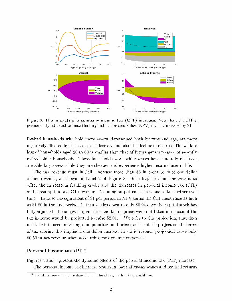
Figure 3: The impacts of a company income tax (CIT) increase. Note that, the CIT ispermanently adjusted to raise the targeted net present value (NPV) revenue increase by $1.

Retired households who hold more assets, determined both by type and age, are more

negatively a�ected by the asset price decrease and also the decline in returns. The welfare

loss of households aged 20 to 60 is smaller than that of future generations or of recently

retired older households. These households work while wages have not fully declined,

are able buy assets while they are cheaper and experience higher returns later in life.

The tax revenue must initially increase more than $3 in order to raise one dollar

of net revenue, as shown in Panel 2 of Figure 3. Such large revenue increase is to

o�set the increase in franking credit and the decreases in personal income tax (PIT)

and consumption tax (CT) revenue. Declining output causes revenue to fall further over

time. To raise the equivalent of $1 per period in NPV terms the CIT must raise as high

as $1.80 in the �rst period. It then settles down to only $0.94 once the capital stock has

fully adjusted. If changes in quantities and factor prices were not taken into account the

tax increase would be projected to raise $2.01.16 We refer to this projection, that does

not take into account changes in quantities and prices, as the static projection. In terms

of tax scoring this implies a one dollar increase in static revenue projection raises only

$0.50 in net revenue when accounting for dynamic responses.

Personal income tax (PIT)

Figures 4 and 7 present the dynamic e�ects of the personal income tax (PIT) increase.

The personal income tax increase results in lower after-tax wages and realised returns

16The static revenue �gure does include the change in franking credit use.

21

on assets for residents. As such households substitute towards leisure and away from

saving. Households not only reduce labour supply over their life but also shift labour

supply from earlier to later in life as they value saving less. When the policy change is

brought in households shift labour supply to later in life causing aggregate labour supply

to decline by more in the medium term than in the long run, as shown in Panel 4 of

Figure 4.

Figure 4: The impacts of a personal income tax (PIT) increase. Note that, the PIT ispermanently adjusted to raise the targeted net present value (NPV) revenue increase by $1.

The decline in labour supply reduces the marginal product of capital and the return

on assets. As such the �rm invests less and the capital stock declines. The distortions to

the household labour supply decision and the savings decision drives the welfare losses.

The tax collects revenue in line with earnings which means lower income and older

households pay less additional tax. As such, the oldest households and those with the

lowest labour productivity are better o� from the policy change due to the increased

transfers. Future high labour productivity households are the most negatively a�ected

as they work with a lower capital stock.

The aggregate marginal excess burden is smaller than that for the company income

tax with welfare losses largely re�ecting income patterns. The smaller aggregate dis-

tortion can also be observed in small capital stock and labour supply changes. The

di�erence between the static revenue estimate and the dynamic estimate is also smaller

for the PIT than the CIT. In terms of tax scoring a PIT increase that is projected to raise

one dollar of static revenue raises $0.73 once the dynamic e�ects are taken into account.

There are limited changes in the other tax bases in response to the PIT increase.

22

Consumption tax (CT)

Figures 5 and 8 display the dynamic e�ects of the consumption tax (CT) increase.

A consumption tax increase raises the cost of consumption and causes substitution

towards leisure. However, unlike the personal income tax, this increase does not sig-

ni�cantly a�ect the inter-temporal savings decision. Households decrease labour supply

more uniformly over their life cycle.

Figure 5: The impacts of consumption tax (CT) increase. Note that, the CT is perma-nently adjusted to raise the targeted net present value (NPV) revenue increase by $1.

The welfare impacts of the CT increase largely mirror the consumption patterns

in the model, as shown in Figure 5. Older households consume less. Younger and

future generations will work with a lower capital stock and are therefore more negatively

a�ected. The change in asset prices also causes a small variation of welfare impacts

across generations.

The aggregate marginal excess burden from raising the CT is smaller than the per-

sonal income tax. The reason is that the CT is collected over a larger base and does not

distort inter-temporal decisions. The older households largely do not pay the personal

income tax; however, they pay the consumption tax. This implies that consumption tax

revenue is collected from a bigger pool of households. The consumption tax on retired

households is e�ectively a lump sum tax as the intra-temporal trade o� between con-

sumption and leisure is eliminated. This implies no distortion. The tax revenue collected

from working households is relatively smaller; and therefore leads a smaller distortion.

A consumption tax increase to raise one dollar using a static model can only raise $0.80

in our dynamic setting, as shown Panel 3 of Figure 5.

23

4.3 Other taxes

In this section we demonstrate that the MEB approach can be used to facilitate the

comparison of a wide range of taxes. We consider other tax instruments that the gov-

ernment can use to raise revenue from taxing �rm or households, including reducing

investment tax credits (ITC), reducing depreciation deductions (DD), raising personal

labour income tax (PLT), and raising personal asset income tax (PAT).

Table 2 reports the marginal excess burden of di�erent taxes. To ease comparison

we also include the marginal excess burdens of the company income tax (CIT) and the

consumption tax (CT). We classify di�erent taxes into two groups: one imposing on the

�rm side and one imposing on the household sides.

Firm HouseholdCIT ITC DD PIT PAT PLT CT

Aggregate $0.83 $1.30 $1.08 $0.34 $0.48 $0.30 $0.24Old $1.32 -$1.86 $0.00 -$0.64 -$0.13 -$0.79 $0.01Young $0.54 -$1.28 -$0.13 $0.09 $0.77 -$0.11 $0.23Future $0.96 $2.19 $1.51 $0.44 $0.45 $0.45 $0.25Type 1 -$0.02 $0.23 $0.12 -$0.32 -$0.29 -$0.32 -$0.16Type 2 $0.73 $1.18 $0.97 $0.27 $0.41 $0.24 $0.18Type 3 $1.75 $2.46 $2.13 $1.04 $1.29 $0.97 $0.70

Table 2: Marginal excess burdens (MEB) of raising extra revenue from di�erent

taxes on the �rm and households. Note that, CIT: Company income tax; ITC: Investmenttax credits; DD: Depreciation deductions; PIT: Personal income tax; PAT: Personal asset incometax; PLT: Personal labour income tax; and CT: Consumption tax.

Overall, we �nd that the taxes legally incident on �rms, including company income

tax, investment tax credit and depreciation deductions result in a higher level of AMEB

than the taxes legally incident on households, including personal income tax, personal

labour income tax, personal asset income tax and consumption tax. Our ranking points

out that an reduction in investment tax credits has the highest AMEB, while raising the

consumption tax has the lowest AMEB. Overall, our results indicate that the marginal

excess burdens of the taxes on the �rm side dominate that of the taxes on the household

side.

Next, we discuss the underlying mechanism behind the excess burden of each tax

separately.

Investment tax credits (ITC)

We consider an experiment where that the share of investment is no longer claimed imme-

diately, but can then be claimed as depreciation deductions later. Reducing investment

tax credits (ITC) lowers the share of investment the �rm can immediately claim as a tax

24

deduction. This means the reduction in the ITC is o�set by increases in depreciation

deductions later, ∆χI = −∆χδ.

The dynamic e�ects of a reduction in ITC are reported in Figure 9. Reducing ICT

raises the cost of investment and results in less investment occurring. The price of assets

also increases but is held down in the near term due to lower capital adjustment costs

from lower investment. In the medium term the price of assets continues to rise consistent

with increasing dividends from the decreasing capital stock and the increasing marginal

product of capital.

Unlike raising the company income tax, reducing the ITC is a boon to retired house-

holds as the price of their assets increases. The welfare of older households increases

through both the asset price increases and increased transfers. It is younger households

and future generations whose welfare is reduced through lower wages due to the lower

capital stock.

The aggregate distortion caused by a reduction in the ITC is larger than for the

company income tax because of the windfall gains to foreigner investors and older house-

holds. Auerbach and Kotliko� (1987) note that, in a closed economy, decreasing the ITC

is similar to moving from a consumption tax to a labour income tax. That is, decreasing

investment incentives shifts the burden of taxation from the old to the young. Reducing

the ITC increases asset prices and acts as a transfer to older households and foreign in-

vestors. The reduction in the ITC only a�ects new capital raising the overall distortion

relative to the company income tax. The net revenue raised falls signi�cantly over time

as reducing the ITC leads to higher depreciation deductions in the future.

Interestingly, while the reduction in the ITC results in largest aggregate welfare losses

many households alive at the time of the policy change are better o�.

Depreciation deductions (DD)

We model a reduction in depreciation deductions (DD) by reducing the share of depre-

ciation deductions claimable, χδ. The dynamic e�ects are reported in Figure 10.

This reduction raises the e�ective tax rate on capital. Lowering depreciation de-

ductions has similar impacts to an increase in the company income tax (CIT) with

investment, the capital stock and wages all falling over time. However, the change in

depreciation deductions only a�ects variable capital and therefore causes a larger aggre-

gate distortion per dollar of revenue. As the depreciation deductions only a�ects variable

capital the value of assets falls by less than under a CIT increase.

The larger per dollar distortion from the depreciation deductions, compared with the

CIT, can be seen in the larger aggregate welfare loss. However, the welfare loss is smaller

for asset rich households at the time of the policy change.

Lastly it is worth noting that the way debt deductions have been modelled here

25

means that a decrease in debt deductibility has the identical impact to lower depreciation

deductions. We have assumed that debt can only be held against variable capital and not

against the value of the �xed factor. Under this assumption lowering debt deductions

only directly a�ects the return to variable capital. If debt were also held against the

�xed factor then lowering debt deductions would be more like a company income tax

increase.

Personal labour income tax (PLT)

We consider an experiment where the government introduces a personal labour income

tax (PLT). In the model, the PLT this is equivalent to a broad payroll tax. The dynamic

e�ects in Figure 11. The PLT decreases the take home wage of households. The impacts

of increasing PLT display characteristics of both the personal income tax (PIT) and

consumption tax (CT) increases. As with the consumption tax, the PLT directly distorts

the consumption leisure trade o�. The tax base of the PLT is relatively smaller than

that of the consumption tax as it only collects taxes from working households.

The aggregate marginal distortion caused by the PLT is lower than the personal in-

come tax but higher than the consumption tax. It is lower than the personal income tax

because it does not a�ect inter-temporal decisions. It is higher than the consumption

tax because it does not collect revenue from older households whose expenditure is in-

elastic. Retired households prefer an the PLT increase to either personal income tax or

consumption tax increases while future households prefer a consumption tax increase.

Personal asset income tax (PAT)

We consider an experiment where the government introduces a personal asset income

tax (PAT) to raise revenue. This tax e�ectively reduces the returns to assets held by

domestic households. The impacts of the PAT increase is equivalent to a decrease in

franking credit deductibility. The MEB for the PAT is equivalent to the MEB of a

reduction in dividend imputation.

Increasing the PAT distorts households' incentives to work and save and lead to

decreases in saving and labour supply. The dynamic e�ects are reported in Figure 12.

In our small open economy model with perfect capital mobility, the decrease in domestic

saving is perfectly o�set by increased foreign investment. However, changes in aggregate

labor supply a�ect the demand for the aggregate capital stock.

The PAT causes the largest aggregate welfare loss among taxes directly imposed on

the households. In addition, the PAT is more distorting than the personal labour income

tax. The PAT is the least preferred tax for the high productivity households because they

hold the most assets and are most negatively a�ected. Meanwhile, the low productivity

26

households prefer the PAT over the personal labour income tax.

5 Sensitivity analysis

In this section we check the robustness of the main results. We consider di�erent model

speci�cations and calibrations: alternative methods to allocation additional tax revenue,

foreign ownership share, the role of �xed factors, franking credits, capital adjustment

speed, economic growth, intertemporal elasticity of substitution and elasticity of labor

supply. Table 3 presents the results from di�erent modelling assumptions.

CIT ITC DD PIT PAT PLT CTBenchmark model $0.83 $1.30 $1.08 $0.34 $0.48 $0.30 $0.24Lump sum redistributive authority $0.82 $1.46 $1.14 $0.36 $0.48 $0.32 $0.24Revenue spent by government $0.54 $0.94 $0.76 $0.13 $0.24 $0.09 $0.04Closed economy $0.63 $0.89 $0.75 $0.41 $0.75 $0.29 $0.24Decreased foreign ownership $1.13 $1.57 $1.41 $0.34 $0.43 $0.32 $0.24Increased foreign ownership share $0.55 $1.02 $0.79 $0.31 $0.53 $0.28 $0.23Increased �xed factors $0.33 $1.32 $1.05 $0.32 $0.38 $0.29 $0.22No �xed factors $1.11 $1.34 $1.17 $0.33 $0.45 $0.30 $0.24No franking credit use $0.70 $1.02 $0.86 $0.42 $0.84 $0.33 $0.25Increased franking credit use -$1.03 -$3.35 -$1.35 $0.20 $0.09 $0.26 $0.21Faster capital adjustment $0.52 $0.97 $0.78 $0.34 $0.54 $0.29 $0.23No growth $0.13 $2.09 $0.31 $0.39 $0.78 $0.29 $0.21Debt tied to equity $0.86 $1.33 $1.10 $0.34 $0.47 $0.30 $0.24Lower intertemporal elasticity $1.03 $1.45 $1.30 $0.29 $0.29 $0.29 $0.23Lower consumption weight in utility $0.85 $1.41 $1.13 $0.43 $0.63 $0.37 $0.29

Table 3: Marginal excess burdens (MEB) of raising extra reveue from di�erent taxes

under di�erent model speci�cations and assumptions. Note that, CIT: Company incometax; ITC: Investment tax credit; DD: Depreciation deductions; PIT: Personal income tax; PAT:personal asset income tax; PLT: Personal labour income tax; and CT: Consumption tax.

Lump Sum Redistributive Authority

The hypothetical Lump Sum Redistributive Authority (LSRA) distributes the additional

revenue so that all households undergo the same welfare change as measured by their

equivalent variation. Unlike the LSRA of Auerbach and Kotliko� (1987) the per period

equivalent variation of all households is equal, not just future households. As all house-

holds experience the same welfare change, the policy causes either a Pareto improvement

or deterioration. The magnitude of the welfare change can be used to assess the e�ciency

of the taxes at the margin.

Compared row 1 and row 2 of Table 3, we �nd that the LSRA changes are generally

slightly larger than the AMEBs under the benchmark speci�cation. The di�erence is

27

in part due to the slightly larger decline in labour supply and output with the LSRA

transfers. E�ective labour supply generally declines further under the LSRA as the

households who bene�t most from the LSRA transfers are higher skill types and those

with more time left in the labour market. This positive income e�ect causes these

households to partake in more leisure and total e�ective labour supply to decline further.

The corresponding decline in output reduces revenue meaning the welfare loss per dollar

of net revenue is slightly larger.

Additional revenue to increase government consumption

In this exercise, we assume that the government allocates additional tax revenue to in-

crease government spending instead of household transfers. The marginal excess burden

in this experiment is taken as the equivalent variation minus the revenue change. As seen

in row 2 of Table 3, the marginal excess burdens of all taxes are consistently smaller,

compared to the baseline scenarios. The main reason is that there is no income e�ect

from the additional transfers in this setting. Without the additional transfers household

supply more labour and revenue increases. As such the distortions per dollar of revenue

are relatively smaller. However, the ranking of tax distortions remains unchanged. The

distributional e�ects are reported in Table 6.

Closed Economy

In the standard model speci�cation the economy is modelled as small and open with

perfect capital mobility. Foreigners are the marginal investor and the �rm maximises it's

value in line with these assumptions. In this sensitivity we instead specify a closed econ-

omy where the stock of assets equal the stock of savings. The �rm is externally �nanced

and maximises it's cum dividend value taking into account taxes paid by households on

dividends and bonds and also the franking credits households receive.17

As seen in row 4 of Table 3, The AMEB for �rm taxes are lower in the closed

economy as the supply of capital is less elastic. As such taxes on capital create less of

a distortion. Further in the closed economy taxing capital at the �rm or the household

level create similar distortions. PAT is most similar in its marginal impacts to decreasing

depreciation or debt deductions.18 CIT creates less of a distortion than PAT because the

PAT allows for no deductions for variable capital which reduce the burden of the tax.

We present the e�ects on skill types and ages in Table 7.

17The interest rate and capital to output ratios vary between the open and close economies. In movingto a closed economy we maintain household parameters such as the discount rate. As the foreign capitalis not available in the closed economy the capital to output ratio is lower and the interest rate is higher.

18The personal asset income tax is a tax on both dividends and interest received but no capital gains.While we could examine the impacts of dividend, interest and capital gains taxes individually a modelsuch as Gourio and Miao (2011) is far better suited to looking at these.

28

Foreign ownership

In the benchmark calibration we assume that foreigners own 17 per cent of assets. In

this sensitivity analysis, we consider di�erent foreign ownership rates.

We �rst lower the initial share of foreign ownership to zero while continuing to assume

perfect capital mobility.19 Table 8 indicates that the AMEB of the �rm taxes is larger

when there is less foreign ownership. The �rm taxes raise less net revenue per unit

of assets when the assets are owned by residents rather than foreigners because of the

dividend imputation system. As a direct result, the distortion per dollar of net revenue

is the higher when foreign ownership is lower. Furthermore, the company income tax

(CIT) raises revenue from the �xed factor which is e�ectively a lump sum transfer from

foreigners to residents. When foreign ownership is lower this transfer is smaller and the

welfare loss from the CIT is larger.

Conversely, we consider an increase in the share of foreign ownership from 17 per

cent to 50 per cent. As seen in Table 9 this has the opposite impact to lowering foreign

ownership. The aggregate distortion from the �rm taxes decreases. The alternate foreign

ownership speci�cations change the magnitude of the MEBs but ordering of the aggre-

gate distortions is preserved. However, the preferences over di�erent tax instruments of

households changes. With increased foreign ownership young household prefer the CIT

to the PIT, PAT and CT.

Fixed factors

In the standard calibration the �xed factor of production contributes 2 per cent of output

calibrated to the contribution of non-residential land. Cao et al. (2015) assume that

natural resources and other �xed factors contribute a further 6 per cent of output. In

this sensitivity analysis, we increase �xed factors contribution to 8 per cent of output

and then decrease it to zero. We summarized the results of the sensitivity analysis with

�xed factors in Tables 11 and 10.

We �nd that the AMEB is lower for the �rm taxes when �xed factors contribute a

larger share of output. Taxing the �xed factor of production is essentially a lump sum

tax. As such when there are more �xed factors the �rm taxes are less distortionary.

Further taxing the �xed factor is partially a transfer from foreigners to residents, this

raises domestic welfare. More �xed factors means there is a larger transfer from foreigners

to residents to o�set the welfare losses due to the distortions of the taxes. While the

ordering of the AMEB for the di�erent taxes is again preserved the impacts on di�erent

groups vary. Under the increased �xed factor speci�cations future households prefer

19The foreign ownership share is lowered by adjusting the assets held by residents. This is done bylowering the households discount rate by changing the parameter β from 0.987 to 0.990.

29

company income tax over the other taxes as it delivers a welfare increase on average.

Without the �xed factor the asset price decrease from an increase in the company

income tax is less than in the benchmark model. As such the welfare loss of households

alive at the time of the policy change is less. When there are no �xed factors distortion

is larger in aggregate due to a more �exible production sector. However, household

alive at the of the policy change would, on average, prefer a consumption tax increase

over a company income tax increase. The consumption tax increase immediately makes

their consumption more expensive while the company income tax increase mainly lowers

future wages.

Franking credits

In the benchmark calibration households are allowed to deduct 37 per cent of franking

credits. In this experiment, we consider two extreme cases: (i) no franking credit use;

and (ii) 100 per cent franking credit use. The results are reported in Tables 12 and 13.

We �nd that in the no franking credit case an increase in the CIT raises more net

revenue. The increase in the CIT is not fully o�set by the franking credit use in the

personal tax system. As a result, the distortion per dollar of revenue is lower. Conversely,

in a setting where 100 per cent franking credit can be used an increase in the CIT results

in a net revenue decrease. The increase in CIT revenue is more than o�set by increased

franking credit use and the decline in the other tax bases. With 100 per cent franking

credit use the CIT is beyond the peak of the La�er curve at that rate. The AMEB is

negative as the revenue change is negative.

Debt to equity ratio

Under the standard model speci�cation we assume a constant share of capital is �nanced

through debt. In this sensitivity we allow the �rm to borrow a �xed share of the value

of its equity. Note that, as the price of equity is greater than the value of capital we

decrease the ratio of debt to equity, so that the overall level of �rm debt is held constant

in both the benchmark model and in this sensitivity analysis. Table 14 displays the

result of this experiment. In this setting when changes in the value of �rm equity result

in changes in the �rm's borrowing capacity. However, the e�ect through this channel is

rather small. There is only a marginal increase in the distortion of the �rm taxes.

Faster capital adjustment

In our benchmark economy, half of the capital stock adjustment in response to a tax

change is completed within approximately 9 years. We adjust the parameters so that

half of capital stock adjustment is completed in 4 years. In particular, we lower the capital

30

adjustment cost parameter ψ from 3.3 to 0.25. When the �rm responds more quickly to

tax changes the distortion of taxation is higher. However, the model also assumes �rms

are not able to deduct adjustment costs from taxable revenue which means adjustment

costs raise the distortion of �rm taxes. As shown in Table 15, under the calibration used

here the second e�ect dominates. A lower adjustment cost leads to a lower distortion for

�rm taxes.

No economic growth

We assume that productivity and populations grow by 1.7 per cent per year in our

benchmark calibration. We now check our results with a no growth assumption. That

is, both population and productivity growth are set to zero, while the risk free interest

rate is maintained. We report the results in Table 16. We �nd that lower growth

decreases the NPV of future revenue and welfare. Distortions that manifest in the future

are given lower weight when growth is lower. When there is no growth the company

income tax (CIT) has the lowest AMEB.

Decreased inter-temporal elasticity of substitution

In the benchmark calibration the inter-temporal elasticity of substitution is 0.4. We test

an inter-temporal elasticity of substitution of 0.2. We report the results in Table 17. We

�nd that reducing the elasticity of inter-temporal substitution reduces the distortion to

saving from the personal income tax (PIT) and the personal asset tax (PAT).

Increased elasticity of labour supply

We conduct a sensitivity analysis with the consumption share of utility. We consider a

lower consumption share of 0.125, compared to 0.25 in the benchmark model. Our simu-

lation results are summarized in Table 18. We �nd that a reduction in the consumption

share of utility increases the uncompensated elasticity of labour supply. The distortions

from taxes that predominantly a�ect the labour supply decision increase.

6 Conclusion

We assess the economic costs of distortionary taxes through the lens of marginal excess

burden in a dynamic general equilibrium, overlapping generations model calibrated to

Australian data. We quantify the aggregate marginal excess burden for di�erent taxes

on the �rm and household sides. We �nd that the taxes which are broadly considered

as falling on capital income are more distorting than the taxes on labour income and

31

consumption. This implies that the overall e�ciency of the tax system can be improved

by relying less on capital income taxes with high marginal excess burden and more on

consumption taxes with low marginal excess burden. More importantly, we are able to

map out the distribution of excess burdens. The uneven distribution of excess burdens

across households and generations implies political challenges when obtaining popular

support for the tax reforms. Those who bene�t the most will likely have to compensate

those who do not bene�t as much.

Our work demonstrates that the marginal excess burden approach can be extended

to a dynamic general equilibrium model �lled with overlapping generations and �rms

with realistic �nancial policy. Moreover, it provides policy makers with a simple but

informative index for assessing the direction of tax policy change as it allows for clear

comparison between di�erent taxes.

The magnitudes of the distortions of the taxes hinge on our modelling assumptions

including market structures and heterogeneity. The core model assumes perfect capital

mobility and using an assumption of imperfect capital mobility would make company

income tax less distorting. The model also assumes a homogeneous good but allowing

for multiple goods and imperfect substitution between domestic and international pro-

duction would introduce further rigidities and lower the measures of distortions. The

set-up of household sector is simpli�ed. While allowing for household heterogeneity by

age and skill we abstract from exogenous income shocks. There is no precautionary sav-

ings motive. Furthermore, we abstract from �rm heterogeneity and �rm �nancing. Our

model can be extended to examine the accuracy of marginal analysis. We leave these

issues for future research.

32

References

Auerbach, Alan J. and James R. Hines, Jr. 2002. Taxation and economic e�ciency. In

Handbook of Public Economics, ed. A. J. Auerbach and M. Feldstein. Vol. 3 Elsevier

Science B. V chapter 21.

Auerbach, Alan J. and Laurence J. Kotliko�. 1987. Dynamic Fiscal Policy. Cambridge

Unversity Press.

Auerbach, Alan J., Laurence J. Kotliko� and Jonathan Skinner. 1983. �The E�ciency

Gains from Dynamic Tax Reform.� International Economic Review 24(1):81�100.

Ballard, Charles L., John B. Shoven and John Whalley. 1985. �General Equilibrium

Computations of the Marginal Welfare Costs of Taxes in the United States.� The

American Economic Review 75(1):128�138.

Cao, Liangyue, Amanda Hosking, Michael Kouparitsas, Damian Mullaly, Xavier Rim-

mer, Qun Shi, Wallace Stark and Sebastian Wende. 2015. �Understanding the

economy-wide e�ciency and incidence of major Australian taxes.� Australian Trea-

sury working paper 1.

Cecchetti, S. G., M. S. Mohanty and F. Zampolli. 2010. �The Future of Public Debt:

Prospects and Implications.� BIS Working Paper No. 300 .

Chamley, Christophe. 1981. �The welfare cost of capital taxation in a growing economy.�

Journal of Political Economy pp. 468�96.

Conesa, Juan Carlos, Sagiri Kitao and Dirk Krueger. 2009. �Taxing Capital? Not a Bad

Idea after All.� American Economic Review 99(1):25�48.

Fehr, Hans and Fabian Kindermann. 2015. �Taxing capital along the transition - Not a

bad idea after all?� Journal of Economic Dynamics and Control 51:64�77.

Feldstein, M. 1978. �The welfare cost of capital income taxation.� Journal of Political

Economy 86:29�51.

Feldstein, M. 1995. �The e�ect of marginal tax rates on taxable income: a panel study

of the 1986 tax reform act.� Journal of Political Economy 103:551�72.

Fullerton, Don and Yolanda Kodrzycki Henderson. 1989. �The Marginal Excess Bur-

den of Di�erent Capital Tax Instruments.� The Review of Economics and Statistics

71(3):435�442.

33

Fuster, L., A. Imrohoroglu and S. Imrohoroglu. 2007. �Altrusim, Incomplete Markets

and Tax Reform.� Working Paper .

Gourio, Francios and Jianjun Miao. 2011. �Transitional dynamics of dividend and capital

gains tax cuts.� Review of Economic Dynamics 14:368�383.

Harberger, A.C. 1964. �The measurement of waste.� American Economic Review 54:58�

76.

Hausman, J.A. 1981. �Exact consumer's surplus and deadweight loss.� American Eco-

nomic Review 71:662�76.

Hines, J.R. 1999. �Three sides of Harberger triangles.� Journal of Economic Perspectives

13:167�88.

IMF. 2010. �Navigating the Fiscal Challenges Ahead.� World Economic and Financial

Surveys .

Imrohoroglu, Selahattin. 1998. �A Quantitative Analysis of Capital Income Taxation.�

International Economic Review 39:307�328.

Judd, Kenneth L. 1985a. �Marginal Excess Burden in a Dynamic Economy.� Economics

Letters 18:213�16.

Judd, Kenneth L. 1985b. �Redistributive Taxation in a Simple Perfect Foresight Model.�

Journal of Public Economics 28:59�83.

Judd, Kenneth L. 1987. �The Welfare Cost of Factor Taxation in a Perfect-Foresight

Model.� Journal of Political Economy 95(4):675�709.

King, M.A. 1983. �Welfare analysis of tax reforms using household data.� Journal of

Public Economics 21:183�214.

Kudrna, G., C. Tran and A. Woodland. 2015. �The Dynamic Fiscal E�ects of Demo-

graphic Shift: The Case of Australia.� Economic Modelling 50:105�122.

Kudrna, G., C. Tran and A. Woodland. Forthcoming. �Facing Demographic Challenges:

Pension Cuts or Tax Hikes.� Macroeconomic Dynamics .

Leeper, Eric M. and Shu-Chun Susan Yang. 2008. �Dynamic scoring: Alternative �nanc-

ing schemes.� Journal of Public Economics 92(1-2):159�182.

Mankiw, N. Gregory and Matthew Weinzierl. 2006. �Dynamic scoring: A back-of-the-

envelope guide.� Journal of Public Economics 90:1415�1433.

34

Miller, Merton H and Franco Modigliani. 1961. �Dividend Policy, Growth, and the

Valuation of Shares.� Journal of Business 34(4):411�33.

Oliner, Stephen, Glenn Rudebusch and Daniel Sichel. 1995. �New and Old Models of

Business Investment: A Comparison of Forecasting Performance.� Journal of Money,

Credit and Banking 27(3):806�826.

Poterba, James M. and Lawrence H. Summers. 1983. �Dividend taxes, corporate invest-

ment, and 'Q'.� Journal of Public Economics 22(2):135�167.

Tran, Chung and Alan Woodland. 2014. �Trade-O�s in Means-Tested Pension Design.�

Journal of Economic Dynamics and Control 47:72�93.

Ventura, Gustavo. 1999. �Flat Tax Reform: A Quantitative Exploration.� Journal of

Economic Dynamics and Control 23(9-10):1425�1458.

35

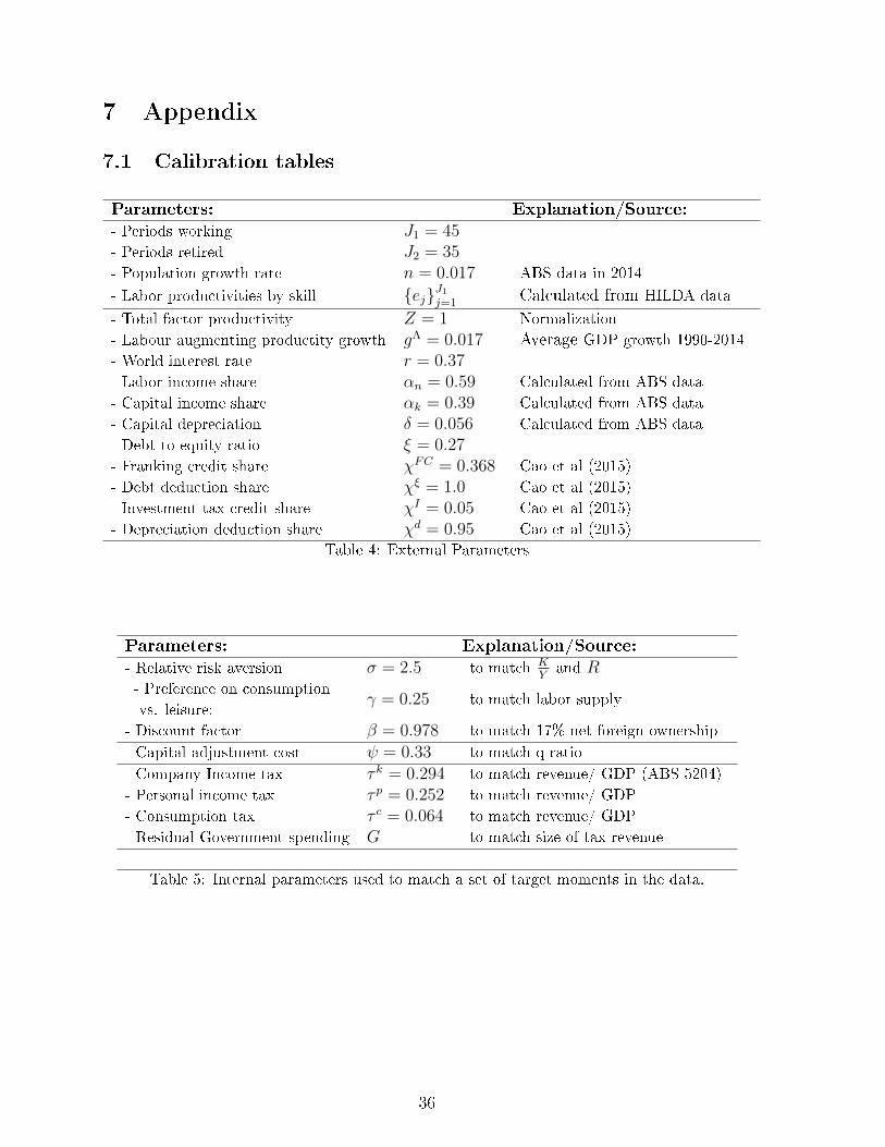
7 Appendix

7.1 Calibration tables

Parameters: Explanation/Source:- Periods working J1 = 45- Periods retired J2 = 35- Population growth rate n = 0.017 ABS data in 2014

- Labor productivities by skill {ej}J1j=1 Calculated from HILDA data

- Total factor productivity Z = 1 Normalization

- Labour augmenting productity growth gΛ = 0.017 Average GDP growth 1990-2014

- World interest rate r = 0.37- Labor income share αn = 0.59 Calculated from ABS data

- Capital income share αk = 0.39 Calculated from ABS data

- Capital depreciation δ = 0.056 Calculated from ABS data

- Debt to equity ratio ξ = 0.27- Franking credit share χFC = 0.368 Cao et al (2015)

- Debt deduction share χξ = 1.0 Cao et al (2015)

- Investment tax credit share χI = 0.05 Cao et al (2015)

- Depreciation deduction share χd = 0.95 Cao et al (2015)

Table 4: External Parameters

Parameters: Explanation/Source:- Relative risk aversion σ = 2.5 to match K

Yand R

- Preference on consumption

vs. leisure:γ = 0.25 to match labor supply

- Discount factor β = 0.978 to match 17% net foreign ownership

- Capital adjustment cost ψ = 0.33 to match q-ratio

- Company Income tax τ k = 0.294 to match revenue/ GDP (ABS 5204)

- Personal income tax τ p = 0.252 to match revenue/ GDP

- Consumption tax τ c = 0.064 to match revenue/ GDP

- Residual Government spending G to match size of tax revenue

Table 5: Internal parameters used to match a set of target moments in the data.

36

7.2 Additional result tables and �gures

CIT ITC DD PIT PAT PLT CTAggregate $0.54 $0.94 $0.76 $0.13 $0.24 $0.09 $0.04Old $0.84 -$1.86 -$0.28 -$0.82 -$0.39 -$0.95 -$0.27Young $0.28 -$1.27 -$0.29 -$0.10 $0.47 -$0.28 $0.02Future $0.66 $1.70 $1.12 $0.22 $0.22 $0.22 $0.05Type 1 -$0.18 $0.04 -$0.06 -$0.43 -$0.40 -$0.43 -$0.30Type 2 $0.46 $0.84 $0.66 $0.07 $0.18 $0.04 -$0.01Type 3 $1.33 $1.92 $1.65 $0.72 $0.94 $0.67 $0.44

Table 6: Marginal excess burdens (MEB) with additional tax revenue allocated to

general government consumption. Note that, CIT: Company income tax; ITC: Investmenttax credits; DD: Depreciation deductions; PIT: Personal income tax; PAT: Personal asset incometax; PLT: Personal labour income tax; and CT: Consumption tax.

CIT ITC DD PIT PAT PLT GSTAggregate $0.63 $0.89 $0.74 $0.41 $0.75 $0.29 $0.24Old $0.15 -$1.36 -$0.50 -$0.52 -$0.51 -$0.53 $0.06Young $0.74 -$0.06 $0.43 $0.13 $0.43 $0.03 $0.29Future $0.76 $1.83 $1.18 $0.68 $1.21 $0.50 $0.25Type 1 -$0.16 -$0.02 -$0.09 -$0.27 -$0.09 -$0.33 -$0.16Type 2 $0.55 $0.80 $0.66 $0.34 $0.67 $0.22 $0.18Type 3 $1.47 $1.87 $1.65 $1.13 $1.66 $0.95 $0.71

Table 7: Marginal excess burdens (MEB) in a closed economy. Note that, CIT: Com-pany income tax; ITC: Investment tax credits; DD: Depreciation deductions; PIT: Personalincome tax; PAT: Personal asset income tax; PLT: Personal labour income tax; and CT: Con-sumption tax.

37

CIT ITC DD PIT PAT PLT CTAggregate $1.13 $1.57 $1.41 $0.34 $0.43 $0.32 $0.24Old $2.41 -$2.24 $0.45 -$0.59 -$0.17 -$0.75 $0.11Young $1.03 -$1.79 -$0.05 $0.11 $0.69 -$0.11 $0.28Future $1.22 $2.75 $1.93 $0.45 $0.41 $0.47 $0.25Type 1 $0.12 $0.35 $0.26 -$0.30 -$0.26 -$0.31 -$0.16Type 2 $1.02 $1.44 $1.28 $0.28 $0.36 $0.25 $0.19Type 3 $2.23 $2.90 $2.65 $1.03 $1.17 $0.99 $0.71

Table 8: Marginal excess burdens (MEB) with lower foreign ownership share. Notethat, CIT: Company income tax; ITC: Investment tax credits; DD: Depreciation deductions;PIT: Personal income tax; PAT: Personal asset income tax; PLT: Personal labour income tax;and CT: Consumption tax.

CIT ITC DD PIT PAT PLT CTAggregate $0.55 $1.02 $0.79 $0.31 $0.53 $0.28 $0.23Old $0.19 -$1.40 -$0.46 -$0.74 -$0.06 -$0.85 -$0.19Young $0.01 -$0.68 -$0.22 $0.04 $0.94 -$0.11 $0.13Future $0.75 $1.61 $1.15 $0.42 $0.49 $0.42 $0.27Type 1 -$0.14 $0.12 -$0.01 -$0.36 -$0.48 -$0.34 -$0.18Type 2 $0.48 $0.93 $0.70 $0.25 $0.45 $0.22 $0.17Type 3 $1.30 $2.00 $1.65 $1.03 $1.59 $0.94 $0.69

Table 9: Marginal excess burdens (MEB) with higher foreign ownership share. Notethat, CIT: Company income tax; ITC: Investment tax credits; DD: Depreciation deductions;PIT: Personal income tax; PAT: Personal asset income tax; PLT: Personal labour income tax;and CT: Consumption tax.

CIT ITC DD PIT PAT PLT CTAggregate $0.33 $1.32 $1.05 $0.32 $0.38 $0.29 $0.22Old $4.63 -$0.71 $1.18 -$0.46 -$0.20 -$0.60 $0.42Young $2.27 -$1.01 $0.29 $0.15 $0.61 -$0.09 $0.41Future -$0.26 $2.18 $1.37 $0.40 $0.37 $0.43 $0.17Type 1 -$0.31 $0.19 $0.05 -$0.28 -$0.22 -$0.31 -$0.16Type 2 $0.26 $1.20 $0.95 $0.26 $0.32 $0.23 $0.16Type 3 $1.03 $2.54 $2.14 $0.98 $1.04 $0.95 $0.67

Table 10: Marginal excess burdens (MEB) with increased �xed factors. Note that,CIT: Company income tax; ITC: Investment tax credits; DD: Depreciation deductions; PIT:Personal income tax; PAT: Personal asset income tax; PLT: Personal labour income tax; andCT: Consumption tax.

38

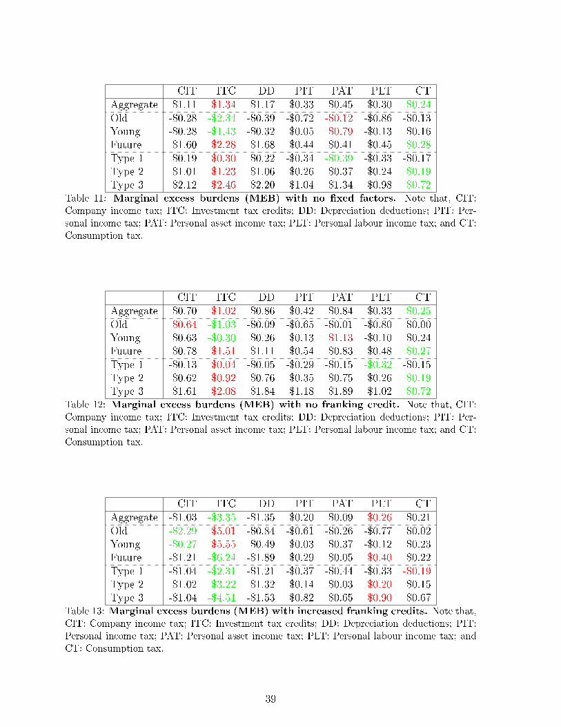
CIT ITC DD PIT PAT PLT CTAggregate $1.11 $1.34 $1.17 $0.33 $0.45 $0.30 $0.24Old -$0.28 -$2.34 -$0.39 -$0.72 -$0.12 -$0.86 -$0.13Young -$0.28 -$1.43 -$0.32 $0.05 $0.79 -$0.13 $0.16Future $1.60 $2.28 $1.68 $0.44 $0.41 $0.45 $0.28Type 1 $0.19 $0.30 $0.22 -$0.34 -$0.39 -$0.33 -$0.17Type 2 $1.01 $1.23 $1.06 $0.26 $0.37 $0.24 $0.19Type 3 $2.12 $2.46 $2.20 $1.04 $1.34 $0.98 $0.72

Table 11: Marginal excess burdens (MEB) with no �xed factors. Note that, CIT:Company income tax; ITC: Investment tax credits; DD: Depreciation deductions; PIT: Per-sonal income tax; PAT: Personal asset income tax; PLT: Personal labour income tax; and CT:Consumption tax.

CIT ITC DD PIT PAT PLT CTAggregate $0.70 $1.02 $0.86 $0.42 $0.84 $0.33 $0.25Old $0.64 -$1.03 -$0.09 -$0.65 -$0.01 -$0.80 $0.00Young $0.63 -$0.30 $0.26 $0.13 $1.13 -$0.10 $0.24Future $0.78 $1.51 $1.11 $0.54 $0.83 $0.48 $0.27Type 1 -$0.13 $0.04 -$0.05 -$0.29 -$0.15 -$0.32 -$0.15Type 2 $0.62 $0.92 $0.76 $0.35 $0.75 $0.26 $0.19Type 3 $1.61 $2.08 $1.84 $1.18 $1.89 $1.02 $0.72

Table 12: Marginal excess burdens (MEB) with no franking credit. Note that, CIT:Company income tax; ITC: Investment tax credits; DD: Depreciation deductions; PIT: Per-sonal income tax; PAT: Personal asset income tax; PLT: Personal labour income tax; and CT:Consumption tax.

CIT ITC DD PIT PAT PLT CTAggregate -$1.03 -$3.35 -$1.35 $0.20 $0.09 $0.26 $0.21Old -$2.29 $5.01 -$0.84 -$0.61 -$0.26 -$0.77 $0.02Young -$0.27 $5.55 $0.49 $0.03 $0.37 -$0.12 $0.23Future -$1.21 -$6.24 -$1.89 $0.29 $0.05 $0.40 $0.22Type 1 -$1.04 -$2.31 -$1.21 -$0.37 -$0.44 -$0.33 -$0.19Type 2 -$1.02 -$3.22 -$1.32 $0.14 $0.03 $0.20 $0.15Type 3 -$1.04 -$4.51 -$1.53 $0.82 $0.65 $0.90 $0.67

Table 13: Marginal excess burdens (MEB) with increased franking credits. Note that,CIT: Company income tax; ITC: Investment tax credits; DD: Depreciation deductions; PIT:Personal income tax; PAT: Personal asset income tax; PLT: Personal labour income tax; andCT: Consumption tax.

39

CIT ITC DD PIT PAT PLT GSTAggregate $0.86 $1.33 $1.11 $0.34 $0.47 $0.30 $0.24Old $1.28 -$1.95 $0.01 -$0.64 -$0.13 -$0.79 $0.01Young $0.54 -$1.28 -$0.10 $0.09 $0.76 -$0.11 $0.23Future $1.01 $2.22 $1.54 $0.44 $0.45 $0.45 $0.25Type 1 -$0.00 $0.24 $0.13 -$0.32 -$0.29 -$0.32 -$0.16Type 2 $0.77 $1.21 $1.00 $0.27 $0.40 $0.24 $0.18Type 3 $1.81 $2.50 $2.17 $1.04 $1.29 $0.97 $0.70

Table 14: Marginal excess burden with debt tied to equity. Note that, CIT: Companyincome tax; ITC: Investment tax credits; DD: Depreciation deductions; PIT: Personal incometax; PAT: Personal asset income tax; PLT: Personal labour income tax; and CT: Consumptiontax.

CIT ITC DD PIT PAT PLT CTAggregate $0.52 $0.97 $0.78 $0.34 $0.54 $0.29 $0.23Old $0.84 -$2.45 -$0.77 -$0.72 -$0.20 -$0.86 -$0.07Young $0.49 -$1.26 -$0.26 $0.10 $0.86 -$0.11 $0.22Future $0.51 $1.66 $1.08 $0.44 $0.51 $0.43 $0.24Type 1 -$0.18 $0.07 -$0.04 -$0.32 -$0.27 -$0.33 -$0.17Type 2 $0.44 $0.87 $0.69 $0.28 $0.46 $0.23 $0.17Type 3 $1.28 $1.95 $1.67 $1.06 $1.41 $0.96 $0.69

Table 15: Marginal excess burdens (MEB) with faster capital adjustment. Note that,CIT: Company income tax; ITC: Investment tax credits; DD: Depreciation deductions; PIT:Personal income tax; PAT: Personal asset income tax; PLT: Personal labour income tax; andCT: Consumption tax.

CIT ITC DD PIT PAT PLT CTAggregate $0.13 $2.09 $0.31 $0.39 $0.78 $0.29 $0.21Old $0.10 -$4.53 -$0.30 -$0.60 $0.06 -$0.78 -$0.07Young -$0.34 -$1.56 -$0.43 $0.27 $1.01 $0.07 $0.20Future $0.91 $9.47 $1.60 $0.80 $0.88 $0.78 $0.29Type 1 -$0.46 $0.67 -$0.36 -$0.23 $0.01 -$0.29 -$0.19Type 2 $0.08 $1.96 $0.25 $0.32 $0.68 $0.23 $0.15Type 3 $0.74 $3.59 $1.01 $1.07 $1.63 $0.92 $0.67

Table 16: Marginal excess burdens (MEB) with no economic growth. Note that,CIT: Company income tax; ITC: Investment tax credits; DD: Depreciation deductions; PIT:Personal income tax; PAT: Personal asset income tax; PLT: Personal labour income tax; andCT: Consumption tax.

40

CIT ITC DD PIT PAT PLT CTAggregate $1.03 $1.45 $1.30 $0.29 $0.29 $0.29 $0.23Old $1.85 -$1.90 $0.28 -$0.64 -$0.24 -$0.78 $0.05Young $0.66 -$1.31 -$0.07 $0.04 $0.54 -$0.13 $0.21Future $1.19 $2.43 $1.79 $0.39 $0.26 $0.44 $0.25Type 1 $0.08 $0.32 $0.23 -$0.33 -$0.36 -$0.32 -$0.16Type 2 $0.93 $1.33 $1.18 $0.22 $0.22 $0.23 $0.17Type 3 $2.05 $2.68 $2.45 $0.96 $0.99 $0.95 $0.69

Table 17: Marginal excess burdens (MEB) with lower intertemporal elasticity. Notethat, CIT: Company income tax; ITC: Investment tax credits; DD: Depreciation deductions;PIT: Personal income tax; PAT: Personal asset income tax; PLT: Personal labour income tax;and CT: Consumption tax.

CIT ITC DD PIT PAT PLT CTAggregate $0.85 $1.41 $1.13 $0.43 $0.63 $0.37 $0.29Old $1.18 -$1.91 -$0.08 -$0.58 $0.01 -$0.76 $0.04Young $0.61 -$1.29 -$0.08 $0.17 $0.96 -$0.06 $0.29Future $0.99 $2.33 $1.57 $0.54 $0.61 $0.53 $0.31Type 1 -$0.06 $0.23 $0.09 -$0.30 -$0.23 -$0.32 -$0.15Type 2 $0.76 $1.29 $1.03 $0.36 $0.55 $0.31 $0.23Type 3 $1.83 $2.67 $2.25 $1.20 $1.55 $1.11 $0.80

Table 18: Marginal excess burdens (MEB) with smaller consumption weight in util-

ity. Note that, CIT: Company income tax; ITC: Investment tax credits; DD: Depreciationdeductions; PIT: Personal income tax; PAT: Personal asset income tax; PLT: Personal labourincome tax; and CT: Consumption tax.

41

Figure 6: The impacts of company income tax (CIT) increase. Note that, the CIT ispermanently adjusted to raise the targeted net present value (NPV) revenue increase by $1.

42

Figure 7: The impact of personal income tax (PIT) increase. Note that, the PIT ispermanently adjusted to raise the targeted net present value (NPV) revenue increase by $1.

43

Figure 8: The impacts of consumption tax (CT) increase. Note that, the CT is perma-nently adjusted to raise the targeted net present value (NPV) revenue increase by $1.

44

Figure 9: The impact of investment tax credit (ITC) reduction.

45

Figure 10: The impacts of debt deduction (DD) reduction.

46

Figure 11: The impacts of personal labour income tax (PLT) increase.

47

Figure 12: The impacts of personal asset income tax (PAT) increase.

48