Tsunami wave impact on walls & beaches - Ocean … wave impact on walls & beaches ... Wave-seabed...
30
Tsunami wave impact on walls & beaches Jannette B. Frandsen 27 Mar. 2014 http://lhe.ete.inrs.ca
Transcript of Tsunami wave impact on walls & beaches - Ocean … wave impact on walls & beaches ... Wave-seabed...

Tsunami wave impact on walls & beaches
Jannette B. Frandsen 27 Mar. 2014http://lhe.ete.inrs.ca
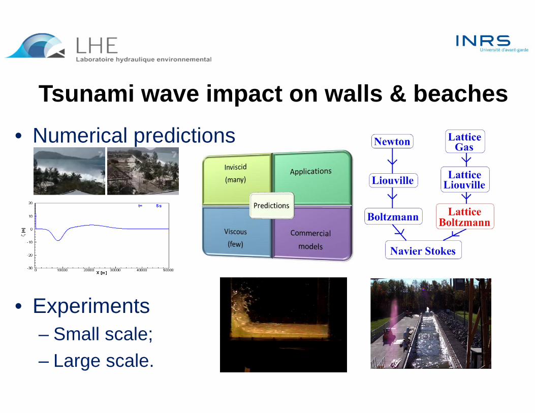
• Numerical predictions
• Experiments – Small scale;– Large scale.
Tsunami wave impact on walls & beaches

Numerical Free-surface models
Airy, Stokes IIStokes III-V, stream functionFully nonlinearNLSW, Boussinesq3rd generation spectral
Large bodies: ships, FPU, fixed offshore platformsOffshore wind farms, tidal machines, WECsOscillations: harbours/Lakes, sloshing, runup/overtoppingMetOcean conditions & Resource assessment
RANS VOFSPH + subgrid scaleLattice Boltzmann
Commercial: Flow3D, Xflow, WAMIT, ANSYS Aqwa, WAM, SWAN.Research: COULWAVE, FUNWAVE, SWAN, MIKE
Inviscid models
Viscous models
Applications
Solvers

• Numerical investigations of VIV & free surface water waves: continuum mechanics models.
• Bridge length/time scales btw. micro and continuum mechanics level.
• Identify numerical model approach aiming at:1. FSI/High Re problems;2. Fr > 1 problems;3. Nonlinear free surface
water wave problems;4. Wave-seabed interactions;5. Water wave bluff body
interactions?
VIV = Vortex Induced Vibrations;FSI = Fluid Structure Interaction.
Traditional research models:
Alternative research models:
Motivation & fundamental questions
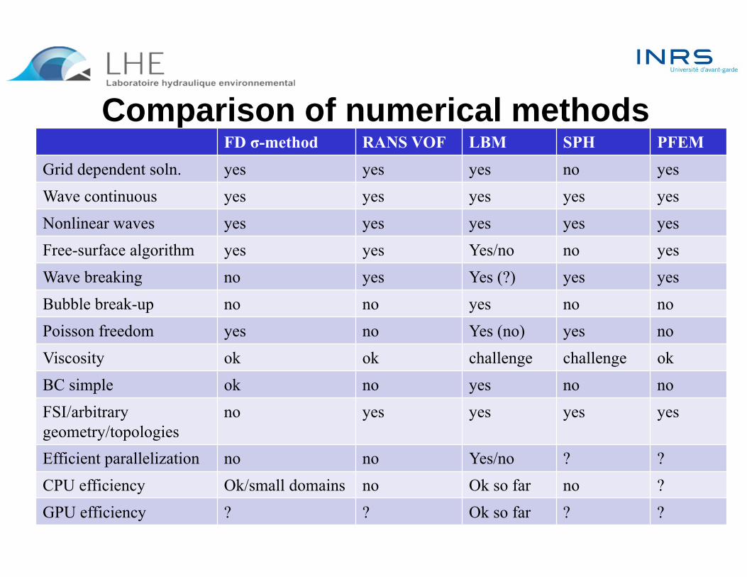
Comparison of numerical methodsFD σ-method RANS VOF LBM SPH PFEM
Grid dependent soln. yes yes yes no yesWave continuous yes yes yes yes yesNonlinear waves yes yes yes yes yesFree-surface algorithm yes yes Yes/no no yesWave breaking no yes Yes (?) yes yesBubble break-up no no yes no noPoisson freedom yes no Yes (no) yes noViscosity ok ok challenge challenge okBC simple ok no yes no noFSI/arbitrary geometry/topologies
no yes yes yes yes
Efficient parallelization no no Yes/no ? ?CPU efficiency Ok/small domains no Ok so far no ?GPU efficiency ? ? Ok so far ? ?

• Why….• Breaking wave predictions,• Local free-surface model and coupling effects.
• “….knowledge and methods established in gas dynamics can be transferred directly to long water waves.” Mei, “The applied dynamics of ocean surface waves”, 1989;• “…..impossible to doubt a close connection btw. mathematical analogy of gas dynamics and the structure underlying long surf on beaches”. Meyer, Physics of Fluids, 1986;
• Wehausen & Laitone, “Surface Waves”, 1960;
• Stoker, “Water Waves”, 1957;
• Courant & Friedrichs, “Supersonic flow and shock waves”, 1948.
• Einstein, H. & Baird, “…surface shock waves on liquids & shocks in compressible gases.” CalTech Report, 1946.
• Riabouchinsky, 1932.
L. Boltzmann
On the Analogy btw. Water waves and gas dynamics theory:
Kinetic modeling approach:

Non-breaking wave models – CPU based• Salmon 1999. Journal of Marine Research 57, 503-535. • Ghidaoui et al. 2001. Intl. J. for Num. Methods in Fluids 35. • Buick & Greated 2003. Physics of Fluids 10 (6), 1490-1511. • Zhou 2004. LB Methods for Shallow Water Flows. Springer. • Zhong et al. 2005. Advances in Atmos. Sciences 22(3). • Ghidaoui et al. 2006. J. Fluids Mechanics 548. • Frandsen 2006. Intl. Journal of CFD 20 (6). • Que & Xu 2006. Intl. J. Num. Meth. in Fluids 50. • Thommes et al. 2007. Intl. J. Num. Meth. in Fluids. • Frandsen 2008. Advanced Numerical Models for Simulating
Tsunami Waves & Runup. Advances in Coastal & Ocean Engrg. World Scientific (10).
• ...... • Parmigiani, A., et al. 2013. Intl. J. Modern Physics C.

Breaking wave models – CPU based

Observations
• Non-breaking wave model:1. NLSW equations;2. No free-surface algorithm.
• Breaking wave model:1. Navier-Stokes equations;2. Free-surface algorithm: Volume of Fluid method

Lattice Boltzmann Model• Fluid motion governed by Navier-Stokes eqn.;
• Particles move along lattice in collision process;
• Collisions allow particles to reach local equilibrium;
• Discretized particle velocity distribution function;
• 3D: ex. 19 or 27 velocities on a cubic lattice;
• Hydrodynamic fields: total depth, velocity and pressure.
ContinuumMolecular Meso
αβ
γ 12
13
7
10
8
9
17
16
18
15
04
11
3
6
2
1
5
14
y
z
x
k
j
i

Collision Integral
• Single time relaxation, - LBGK model, after Bhatnagar et al. (1954) ;
• Multi Relaxation Times, MRT models.
Approximations:
Original Boltzmann Equation
L. Boltzmann
Collisions Propagation

Lattice Boltzmann Model in Shallow water
i

LBGK model example
2 2 20 0
0 0 2 2
( ) ( ) ( )2
eqi i i
g h t h tf h u ux x
2 2 2
0 0 01,2 2 2
( ) ( ) ( ) ( )4 2 2
eq ii i i i
g h t h tu h tf c u ux x x
2
00
ii
f h
Discrete velocity model (D1Q3)
The macroscopic variables
2
00
1( ) i i
iu c f
h
j
f1f
2
f1
f2
(1 − )α f1(1 − )α f
2
f2αf
1α
x + xΔ
t + tΔ
t
+ c _ c
f2
f1(= c )
Δ(x + 2
x)j
x
t
(Soln.: 0. Initial conditions; 1. Calculate feq; 2. Compute fi.)

• Free-surface: no algorithm is prescribed in non-overturning wave model;
• Wave run-up: dry/wet phase (h 0):Automatically handled (i.e., thin film: h~10-5m); Shoreline algorithm; “Slot method”.
z
x L
z0h0hb
h0/L0 0 , ε = a/h0 = O(1)
Z0 = 5000 m
∂hb/∂x = 1/10
L = 50 km
• Problem Set-up
Long Wave Run-up Studies

Initial Conditions & Boundaries

Near-shore view:
Domain view:
FDLB model 5,000 nodes

Validation
FDLB model 5,000 nodes

−400 −200 0 200 400−20
−10
0
10
20
x [m]
u s [m/s
]
−400 −200 0 200 400−20
−10
0
10
20
x [m]
u s [m/s
]
Other initial wave forms
−400 −200 0 200 400−20
−10
0
10
20
x [m]
u s [m/s
]
−400 −200 0 200 400−20
−10
0
10
20
x [m]u s [m
/s]
A B
C D
−0.050 5 7
x 104
−4
0
10
x [m]
ζ [m
]
−0.050 5 7
x 104
−10
0
4
x [m]
ζ [m
]
−0.050 5 7
x 104
−4
0
10
x [m]
ζ [m
]
A
B
C
D
, FD LB model , Carrier et al., JFM (2003)

Experimental set-up and definitions
1 m
/4b
/4b
/2
l /2 l /2
x
y
1
3
2
Sway
Surge
1 m
b
b
1
h 2
U0h0
uy
ζ
h
Wave gauge
Small Scale Testing

Large sway motion
ah/b=0.02 ah/b=0.05 ah/b=0.1
h0/b=0.05
Fr1=1.1h1/h2=1.6
Fr1=1.3h1/h2=2.2
Fr1=1.4h1/h2=6.9
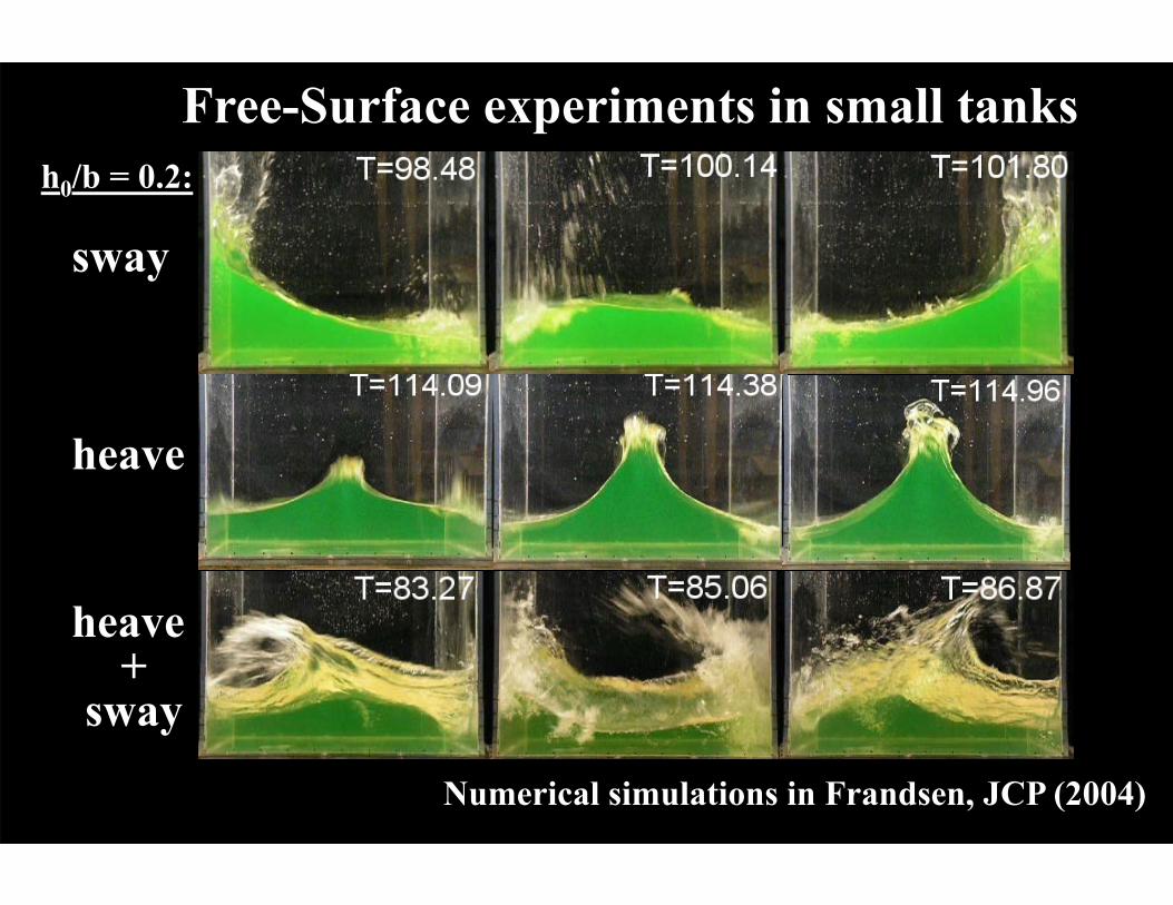
sway
heave
heave +
sway
h0/b = 0.2:
Numerical simulations in Frandsen, JCP (2004)
Free-Surface experiments in small tanks

0.8 1 1.2 0
0.2
0.4
ωh/ω
1
ζ max
/b
0.8 1 1.2 0
0.2
0.4
ωh/ω
1ζ m
ax/b
Horizontal moving tank with forcing frequency ωh-x -, Analytical 3rd order solution; -o-, numerical nonlinear potential flow soln,
ah/b = 0.003 (Frandsen, JCP’04); - - , experimental solution (ah/b = 0.003);
, experimental solution (ah/b = 0.006);.
h0/b = 0.2 h0/b = 0.6Sloshing in tank: physical vs. numerical test soln
2n1
n
ζ
hs
still water level
Δσ = 1
XΔ = 12
m1 m
(b)(a)
σ
X
mapping
b
z
Initial profile
x
●, wave breaking

Free-surface VOF LB model
• Free-surface algorithm using Volume of Fluid (VOF) method (Ginzburg & Steiner, 2002)
• D3Q27 lattice (recovers the Navier-Stokes equations)
• Mesh: Structured, Octree grids
• Adaptivity: mesh adapts to the wake while the flow develops. (constraints on the local dimensionless vorticity.)
• Large Eddy Simulation (local wall adapting eddy viscosity model)
• Multiple Relaxation Time
Commercially available

Wave runup on beaches
Wave tank: 37.7 m 0.61 m 0.39 mAfter Synolakis, JFM (1987)
LB solution:
Smooth Beach: 1:19.85
Runup height vs. wave height
H/d =0.5, R/d = 1.511
LB VOF solns
800-900 k elements

ExpériencesLarge Scale Testing04
• Depth/width: 5 m; Length: 120 m • Water depth: 2.5 - 3.5 m • Wave period: 3 - 10 s.• Wavemaker (piston): max. stroke length/velocity: 4 m, 4 m/s.• Initial conditions:
Regular/ irregular waves & user-defined functions,e.g., landslide & earthquake-generated tsunami.
• The flume is designed for modeling the interactions of waves, tides, currents, and sediment transport.
• Instrumentation: ADP, ADV, Aquadopp, turbidity-, water level -and pressure sensors. multibeam system (bathymetry).

Expériences
Wave impact on walls04 octobre 2013
Large Scale Testing04
~ 10 m
~ 3 – 4 MPa in few ms.

Beach stability experiments
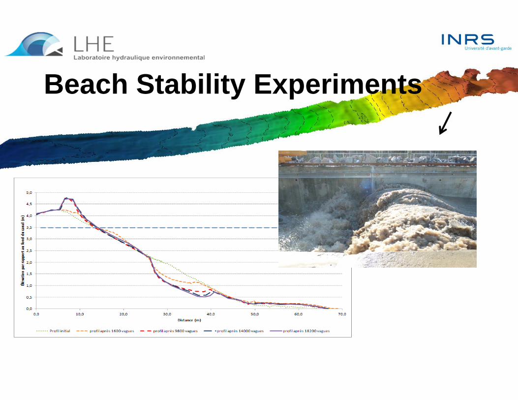
Beach Stability Experiments

Concluding thoughtsNear-shore
HydrodynamicModels
• Compatible with other nonlinear shallow water solvers;• Hybrid models to bridge length/time scales;• Assist in design of coastal/harbor structures;• Simplified models in the context of warning systems,
evacuation and inundation mapping.
Kinetic approaches when viscosity and complex fluid mixing and structural response as coupled interactions matters.

Questions?
Jannette B. Frandsen 27 Mar. 2014http://lhe.ete.inrs.ca
What’s next?