Tseng, W., Penzien, J. Soil-Foundation-Structure Interaction. Bridge …freeit.free.fr/Bridge...
53
Tseng, W., Penzien, J. "Soil-Foundation-Structure Interaction." Bridge Engineering Handbook. Ed. Wai-Fah Chen and Lian Duan Boca Raton: CRC Press, 2000
Transcript of Tseng, W., Penzien, J. Soil-Foundation-Structure Interaction. Bridge …freeit.free.fr/Bridge...

Tseng, W., Penzien, J. "Soil-Foundation-Structure Interaction." Bridge Engineering Handbook. Ed. Wai-Fah Chen and Lian Duan Boca Raton: CRC Press, 2000

42Soil–Foundation–
Structure Interaction
42.1 Introduction
42.2 Description of SFSI ProblemsBridge Foundation Types • Definition of SFSI Problems • Demand vs. Capacity Evaluations
42.3 Current State of the PracticeElastodynamic Method • Empirical p–y Method
42.4 Seismic Inputs to SFSI SystemFree-Field Rock-Outcrop Motions at Control Point Location • Free-Field Rock-Outcrop Motions at Pier Support Locations • Free-Field Soil Motions
42.5 Characterization of Soil–Foundation SystemElastodynamic Model • Empirical p–y Model • Hybrid Model
42.6 Demand Analysis ProceduresEquations of Motion • Solution Procedures
42.7 Demand Analysis ExamplesCaisson Foundation • Slender-Pile Group Foundation • Large-Diameter Shaft Foundation
42.8 Capacity Evaluations
42.9 Concluding Statements
42.1 Introduction
Prior to the 1971 San Fernando, California earthquake, nearly all damages to bridges duringearthquakes were caused by ground failures, such as liquefaction, differential settlement, slides,and/or spreading; little damage was caused by seismically induced vibrations. Vibratory responseconsiderations had been limited primarily to wind excitations of large bridges, the great importanceof which was made apparent by failure of the Tacoma Narrows suspension bridge in the early 1940s,and to moving loads and impact excitations of smaller bridges.
The importance of designing bridges to withstand the vibratory response produced duringearthquakes was revealed by the 1971 San Fernando earthquake during which many bridge struc-tures collapsed. Similar bridge failures occurred during the 1989 Loma Prieta and 1994 Northridge,California earthquakes, and the 1995 Kobe, Japan earthquake. As a result of these experiences, muchhas been done recently to improve provisions in seismic design codes, advance modeling and analysis
Wen-Shou TsengInternational Civil Engineering
Consultants, Inc.
Joseph PenzienInternational Civil Engineering
Consultants, Inc.
© 2000 by CRC Press LLC

procedures, and develop more effective detail designs, all aimed at ensuring that newly designedand retrofitted bridges will perform satisfactorily during future earthquakes.
Unfortunately, many of the existing older bridges in the United States and other countries, whichare located in regions of moderate to high seismic intensity, have serious deficiencies which threatenlife safety during future earthquakes. Because of this threat, aggressive actions have been taken inCalifornia, and elsewhere, to retrofit such unsafe bridges bringing their expected performancesduring future earthquakes to an acceptable level. To meet this goal, retrofit measures have beenapplied to the superstructures, piers, abutments, and foundations.
It is because of this most recent experience that the importance of coupled soil–foundation–struc-ture interaction (SFSI) on the dynamic response of bridge structures during earthquakes has beenfully realized. In treating this problem, two different methods have been used (1) the “elastodynamic”method developed and practiced in the nuclear power industry for large foundations and (2) theso-called empirical p–y method developed and practiced in the offshore oil industry for pile foun-dations. Each method has its own strong and weak characteristics, which generally are opposite tothose of the other, thus restricting their proper use to different types of bridge foundation. Bycombining the models of these two methods in series form, a hybrid method is reported hereinwhich makes use of the strong features of both methods, while minimizing their weak features.While this hybrid method may need some further development and validation at this time, it isfundamentally sound; thus, it is expected to become a standard procedure in treating seismic SFSIof large bridges supported on different types of foundation.
The subsequent sections of this chapter discuss all aspects of treating seismic SFSI by the elastody-namic, empirical p–y, and hybrid methods, including generating seismic inputs, characterizingsoil–foundation systems, conducting force–deformation demand analyses using the substructuringapproach, performing force–deformation capacity evaluations, and judging overall bridge performance.
42.2 Description of SFSI Problems
The broad problem of assessing the response of an engineered structure interacting with its sup-porting soil or rock medium (hereafter called soil medium for simplicity) under static and/ordynamic loadings will be referred here as the soil–structure interaction (SSI) problem. For a buildingthat generally has its superstructure above ground fully integrated with its substructure below,reference to the SSI problem is appropriate when describing the problem of interaction betweenthe complete system and its supporting soil medium. However, for a long bridge structure, consistingof a superstructure supported on multiple piers and abutments having independent and oftendistinct foundation systems which in turn are supported on the soil medium, the broader problemof assessing interaction in this case is more appropriately and descriptively referred to as thesoil–foundation–structure interaction (SFSI) problem. For convenience, the SFSI problem can beseparated into two subproblems, namely, a soil–foundation interaction (SFI) problem and a foun-dation–structure interaction (FSI) problem. Within the context of SFSI, the SFI part of the totalproblem is the one to be emphasized, since, once it is solved, the FSI part of the total problem canbe solved following conventional structural response analysis procedures. Because the interactionbetween soil and the foundations of a bridge makes up the core of an SFSI problem, it is useful toreview the different types of bridge foundations that may be encountered in dealing with thisproblem.
42.2.1 Bridge Foundation Types
From the perspective of SFSI, the foundation types commonly used for supporting bridge piers canbe classified in accordance with their soil-support configurations into four general types: (1) spreadfootings, (2) caissons, (3) large-diameter shafts, and (4) slender-pile groups. These types as describedseparately below are shown in Figure 42.1.
© 2000 by CRC Press LLC
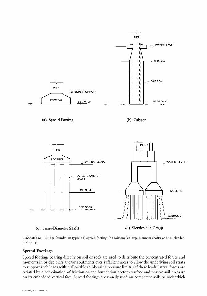
Spread FootingsSpread footings bearing directly on soil or rock are used to distribute the concentrated forces andmoments in bridge piers and/or abutments over sufficient areas to allow the underlying soil stratato support such loads within allowable soil-bearing pressure limits. Of these loads, lateral forces areresisted by a combination of friction on the foundation bottom surface and passive soil pressureon its embedded vertical face. Spread footings are usually used on competent soils or rock which
FIGURE 42.1 Bridge foundation types: (a) spread footing; (b) caisson; (c) large-diameter shafts; and (d) slender-pile group.
© 2000 by CRC Press LLC

have high allowable bearing pressures. These foundations may be of several forms, such as (1)isolated footings, each supporting a single column or wall pier; (2) combined footings, each sup-porting two or more closely spaced bridge columns; and (3) pedestals which are commonly usedfor supporting steel bridge columns where it is desirable to terminate the structural steel abovegrade for corrosion protection. Spread footings are generally designed to support the superimposedforces and moments without uplifting or sliding. As such, inelastic action of the soils supportingthe footings is usually not significant.
CaissonsCaissons are large structural foundations, usually in water, that will permit dewatering to provide a drycondition for excavation and construction of the bridge foundations. They can take many forms to suitspecific site conditions and can be constructed of reinforced concrete, steel, or composite steel andconcrete. Most caissons are in the form of a large cellular rectangular box or cylindrical shell structurewith a sealed base. They extend up from deep firm soil or rock-bearing strata to above mudline wherethey support the bridge piers. The cellular spaces within the caissons are usually flooded and filled withsand to some depth for greater stability. Caisson foundations are commonly used at deep-water siteshaving deep soft soils. Transfer of the imposed forces and moments from a single pier takes place bydirect bearing of the caisson base on its supporting soil or rock stratum and by passive resistance of theside soils over the embedded vertical face of the caisson. Since the soil-bearing area and the structuralrigidity of a caisson is very large, the transfer of forces from the caisson to the surrounding soil usuallyinvolves negligible inelastic action at the soil–caisson interface.
Large-Diameter ShaftsThese foundations consist of one or more large-diameter, usually in the range of 4 to 12 ft (1.2 to3.6 m), reinforced concrete cast-in-drilled-hole (CIDH) or concrete cast-in-steel-shell (CISS) piles.Such shafts are embedded in the soils to sufficient depths to reach firm soil strata or rock where ahigh degree of fixity can be achieved, thus allowing the forces and moments imposed on the shaftsto be safely transferred to the embedment soils within allowable soil-bearing pressure limits and/orallowable foundation displacement limits. The development of large-diameter drilling equipmenthas made this type of foundation economically feasible; thus, its use has become increasinglypopular. In actual applications, the shafts often extend above ground surface or mudline to form asingle pier or a multiple-shaft pier foundation. Because of their larger expected lateral displacementsas compared with those of a large caisson, a moderate level of local soil nonlinearities is expectedto occur at the soil–shaft interfaces, especially near the ground surface or mudline. Such nonlin-earities may have to be considered in design.
Slender-Pile GroupsSlender piles refer to those piles having a diameter or cross-sectional dimensions less than 2 ft (0.6 m).These piles are usually installed in a group and provided with a rigid cap to form the foundation of abridge pier. Piles are used to extend the supporting foundations (pile caps) of a bridge down throughpoor soils to more competent soil or rock. The resistance of a pile to a vertical load may be essentiallyby point bearing when it is placed through very poor soils to a firm soil stratum or rock, or by frictionin case of piles that do not achieve point bearing. In real situations, the vertical resistance is usuallyachieved by a combination of point bearing and side friction. Resistance to lateral loads is achieved bya combination of soil passive pressure on the pile cap, soil resistance around the piles, and flexuralresistance of the piles. The uplift capacity of a pile is generally governed by the soil friction or cohesionacting on the perimeter of the pile. Piles may be installed by driving or by casting in drilled holes. Drivenpiles may be timber piles, concrete piles with or without prestress, steel piles in the form of pipe sections,or steel piles in the form of structural shapes (e.g., H shape). Cast-in-drilled-hole piles are reinforcedconcrete piles installed with or without steel casings. Because of their relatively small cross-sectionaldimensions, soil resistance to large pile loads usually develops large local soil nonlinearities that must
© 2000 by CRC Press LLC
be considered in design. Furthermore, since slender piles are normally installed in a group, mutualinteractions among piles will reduce overall group stiffness and capacity. The amounts of these reductionsdepend on the pile-to-pile spacing and the degree ofsoil nonlinearity developed in resisting the loads.
42.2.2 Definition of SFSI Problem
For a bridge subjected to externally applied static and/or dynamic loadings on the abovegroundportion of the structure, the SFSI problem involves evaluation of the structural performance(demand/capacity ratio) of the bridge under the applied loadings taking into account the effect ofSFI. Since in this case the ground has no initial motion prior to loading, the effect of SFI is toprovide the foundation–structure system with a flexible boundary condition at the soil–foundationinterface location when static loading is applied and a compliant boundary condition when dynamicloading is applied. The SFI problem in this case therefore involves (1) evaluation of the soil–foun-dation interface boundary flexibility or compliance conditions for each bridge foundation, (2)determination of the effects of these boundary conditions on the overall structural response of thebridge (e.g., force, moment, or deformation) demands, and (3) evaluation of the resistance capacityof each soil–foundation system that can be compared with the corresponding response demand inassessing performance. That part of determining the soil–foundation interface boundary flexibilitiesor compliances will be referred to subsequently in a gross term as the “foundation stiffness orimpedance problem”; that part of determining the structural response of the bridge as affected bythe soil–foundation boundary flexibilities or compliances will be referred to as the “founda-tion–structure interaction problem”; and that part of determining the resistance capacity of thesoil–foundation system will be referred to as the “foundation capacity problem.”
For a bridge structure subjected to seismic conditions, dynamic loadings are imposed on thestructure. These loadings, which originate with motions of the soil medium, are transmitted to thestructure through its foundations; therefore, the overall SFSI problem in this case involves, inaddition to the foundation impedance, FSI, and foundation capacity problems described above, theevaluation of (1) the soil forces acting on the foundations as induced by the seismic ground motions,referred to subsequently as the “seismic driving forces,” and (2) the effects of the free-field ground-motion-induced soil deformations on the soil–foundation boundary compliances and on the capac-ity of the soil–foundation systems. In order to evaluate the seismic driving forces on the foundationsand the effects of the free-field ground deformations on compliances and capacities of the soil–foun-dation systems, it is necessary to determine the variations of free-field motion within the groundregions which interact with the foundations. This problem of determining the free-field groundmotion variations will be referred to herein as the “free-field site response problem.” As will beshown later, the problem of evaluating the seismic driving forces on the foundations is equivalentto determining the “effective or scattered foundation input motions” induced by the free-field soilmotions. This problem will be referred to here as the “foundation scattering problem.”
Thus, the overall SFSI problem for a bridge subjected to externally applied static and/or dynamicloadings can be separated into the evaluation of (1) foundation stiffnesses or impedances, (2)foundation–structure interactions, and (3) foundation capacities. For a bridge subjected to seismicground motion excitations, the SFSI problem involves two additional steps, namely, the evaluationof free-field site response and foundation scattering. When solving the total SFSI problem, the effectsof the nonzero soil deformation state induced by the free-field seismic ground motions should beevaluated in all five steps mentioned above.
42.2.3 Demand vs. Capacity Evaluations
As described previously, assessing the seismic performance of a bridge system requires evaluationof SFSI involving two parts. One part is the evaluation of the effects of SFSI on the seismic-responsedemands within the system; the other part is the evaluation of the seismic force and/or deformation
© 2000 by CRC Press LLC
capacities within the system. Ideally, a well-developed methodology should be one that is capableof solving these two parts of the problem concurrently in one step using a unified suitable modelfor the system. Unfortunately, to date, such a unified method has not yet been developed. Becauseof the complexities of a real problem and the different emphases usually demanded of the solutionsfor the two parts, different solution strategies and methods of analysis are warranted for solvingthese two parts of the overall SFSI problem. To be more specific, evaluation on the demand side ofthe problem is concerned with the overall SFSI system behavior which is controlled by the mass,damping (energy dissipation), and stiffness properties, or, collectively, the impedance properties,of the entire system; and, the solution must satisfy the dynamic equilibrium and compatibilityconditions of the global system. This system behavior is not sensitive, however, to approximationsmade on local element behavior; thus, its evaluation does not require sophisticated characterizationsof the detailed constitutive relations of its local elements. For this reason, evaluation of demand hasoften been carried out using a linear or equivalent linear analysis procedure. On the contrary,evaluation of capacity must be concerned with the extreme behavior of local elements or subsystems;therefore, it must place emphasis on the detailed constitutive behaviors of the local elements orsubsystems when deformed up to near-failure levels. Since only local behaviors are of concern, theevaluation does not have to satisfy the global equilibrium and compatibility conditions of the systemfully. For this reason, evaluation of capacity is often obtained by conducting nonlinear analyses ofdetailed local models of elements or subsystems or by testing of local members, connections, orsub-assemblages, subjected to simple pseudo-static loading conditions.
Because of the distinct differences between effective demand and capacity analyses as describedabove, the analysis procedures presented subsequently differentiate between these two parts of theoverall SFSI problem.
42.3 Current State-of-the-Practice
The evaluation of SFSI effects on bridges located in regions of high seismicity has not received asmuch attention as for other critical engineered structures, such as dams, nuclear facilities, andoffshore structures. In the past, the evaluation of SFSI effects for bridges has, in most cases, beenregarded as a part of the bridge foundation design problem. As such, emphasis has been placed onthe evaluation of load-resisting capacities of various foundation systems with relatively little atten-tion having been given to the evaluation of SFSI effects on seismic-response demands within thecomplete bridge system. Only recently has formal SSI analysis methodologies and procedures,developed and applied in other industries, been adopted and applied to seismic performanceevaluations of bridges [1], especially large important bridges [2,3].
Even though the SFSI problems for bridges pose their own distinct features (e.g., multipleindependent foundations of different types supported in highly variable soil conditions rangingfrom hard to very soft), the current practice is to adopt, with minor modifications, the samemethodologies and procedures developed and practiced in other industries, most notably, thenuclear power and offshore oil industries. Depending upon the foundation type and its soil-supportcondition, the procedures currently being used in evaluating SFSI effects on bridges can broadly beclassified into two main methods, namely, the so-called elastodynamic method that has beendeveloped and practiced in the nuclear power industry for large foundations, and the so-calledempirical p–y method that has been developed and practiced in the offshore oil industry for pilefoundations. The bases and applicabilities of these two methods are described separately below.
42.3.1 Elastodynamic Method
This method is based on the well-established elastodynamic theory of wave propagation in a linearelastic, viscoelastic, or constant-hysteresis-damped elastic half-space soil medium. The fundamentalelement of this method is the constitutive relation between an applied harmonic point load and
© 2000 by CRC Press LLC
the corresponding dynamic response displacements within the medium called the dynamic Green’sfunctions. Since these functions apply only to a linear elastic, visoelastic, or constant-hysteresis-damped elastic medium, they are valid only for linear SFSI problems. Since application of theelastodynamic method of analysis uses only mass, stiffness, and damping properties of an SFSIsystem, this method is suitable only for global system response analysis applications. However, byadopting the same equivalent linearization procedure as that used in the seismic analysis of free-field soil response, e.g., that used in the computer program SHAKE [4], the method has beenextended to one that can accommodate global soil nonlinearities, i.e., those nonlinearities inducedin the free-field soil medium by the free-field seismic waves [5].
Application of the elastodynamic theory to dynamic SFSI started with the need for solvingmachine–foundation vibration problems [6]. Along with other rapid advances in earthquake engineer-ing in the 1970s, application of this theory was extended to solving seismic SSI problems for buildingstructures, especially those of nuclear power plants [7–9]. Such applications were enhanced by concur-rent advances in analysis techniques for treating soil dynamics, including development of the complexmodulus representation of dynamic soil properties and use of the equivalent linearization techniquefor treating ground-motion-induced soil nonlinearities [10–12]. These developments were furtherenhanced by the extensive model calibration and methodology validation and refinement efforts carriedout in a comprehensive large-scale SSI field experimental program undertaken by the Electric PowerResearch Institute (EPRI) in the 1980s [13]. All of these efforts contributed to advancing the elastody-namic method of SSI analysis currently being practiced in the nuclear power industry [5].
Because the elastodynamic method of analysis is capable of incorporating mass, stiffness, anddamping characteristics of each soil, foundation, and structure subsystem of the overall SFSI system,it is capable of capturing the dynamic interactions between the soil and foundation subsystems andbetween the foundations and structure subsystem; thus, it is suitable for seismic demand analyses.However, since the method does not explicitly incorporate strength characteristics of the SFSIsystem, it is not suitable for capacity evaluations.
As previously mentioned in Section 42.2.1, there are four types of foundation commonly usedfor bridges: (1) spread footings, (2) caissons, (3) large-diameter shafts, and (4) slender-pile groups.Since only small local soil nonlinearities are induced at the soil–foundation interfaces of spreadfootings and caissons, application of the elastodynamic method of seismic demand analysis of thecomplete SFSI system is valid. However, the validity of applying this method to large-diameter shaftfoundations depends on the diameter of the shafts and on the amplitude of the imposed loadings.When the shaft diameter is large so that the load amplitudes produce only small local soil nonlin-earities, the method is reasonably valid. However, when the shaft diameter is relatively small, thelarger-amplitude loadings will produce local soil nonlinearities sufficiently large to require that themethod be modified as discussed subsequently. Application of the elastodynamic method to slender-pile groups is usually invalid because of the large local soil nonlinearities which develop near thepile boundaries. Only for very low amplitude loadings can the method be used for such foundations.
42.3.2 Empirical “p-y” Method
This method was originally developed for the evaluation of pile–foundation response due to lateralloads [14–16] applied externally to offshore structures. As used, it characterizes the lateral soilresistance per unit length of pile, p, as a function of the lateral displacement, y. The p–y relation isgenerally developed on the basis of an empirical curve which reflects the nonlinear resistance of thelocal soil surrounding the pile at a specified depth (Figure 42.2). Construction of the curve dependsmainly on soil material strength parameters, e.g., the friction angle, φ, for sands and cohesion, c,for clays at the specified depth. For shallow soil depths where soil surface effects become important,construction of these curves also depends on the local soil failure mechanisms, such as failure by apassive soil resistance wedge. Typical p–y curves developed for a pile at different soil depths areshown in Figure 42.3. Once the set of p–y curves representing the soil resistances at discrete values
© 2000 by CRC Press LLC
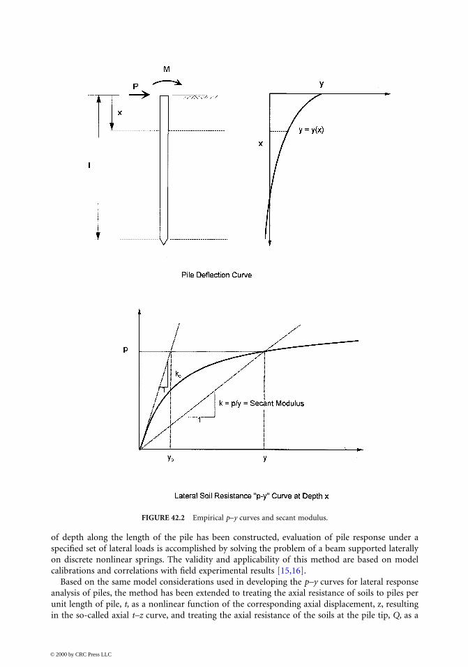
of depth along the length of the pile has been constructed, evaluation of pile response under aspecified set of lateral loads is accomplished by solving the problem of a beam supported laterallyon discrete nonlinear springs. The validity and applicability of this method are based on modelcalibrations and correlations with field experimental results [15,16].
Based on the same model considerations used in developing the p–y curves for lateral responseanalysis of piles, the method has been extended to treating the axial resistance of soils to piles perunit length of pile, t, as a nonlinear function of the corresponding axial displacement, z, resultingin the so-called axial t–z curve, and treating the axial resistance of the soils at the pile tip, Q, as a
FIGURE 42.2 Empirical p–y curves and secant modulus.
© 2000 by CRC Press LLC

nonlinear function of the pile tip axial displacement, d, resulting in the so-called Q–d curve. Again,the construction of the t–z and Q–d curves for a soil-supported pile is based on empirical curvilinearforms and the soil strength parameters as functions of depth. By utilizing the set of p–y, t–z, andQ–d curves developed for a pile foundation, the response of the pile subjected to general three-dimensional (3-D) loadings applied at the pile head can be solved using the model of a 3-D beamsupported on discrete sets of nonlinear lateral p–y, axial t–z, and axial Q–d springs. The method asdescribed above for solving a soil-supported pile foundation subjected to applied loadings at thepile head is referred to here as the empirical p–y method, even though it involves not just the lateralp–y curves but also the axial t–z and Q–d curves for characterizing the soil resistances.
Since this method depends primarily on soil-resistance strength parameters and does not incor-porate soil mass, stiffness, and damping characteristics, it is, strictly speaking, only applicable forcapacity evaluations of slender-pile foundations and is not suitable for seismic demand evaluationsbecause, as mentioned previously, a demand evaluation for an SFSI system requires the incorpora-tion of the mass, stiffness, and damping properties of each of the constituent parts, namely, thesoil, foundation, and structure subsystems.
Even though the p–y method is not strictly suited to demand analyses, it is current practice inperforming seismic-demand evaluations for bridges supported on slender-pile group foundationsto make use of the empirical nonlinear p–y, t–z, and Q–d curves in developing a set of equivalentlinear lateral and axial soil springs attached to each pile at discrete elevations in the foundation.The soil–pile systems developed in this manner are then coupled with the remaining bridge structureto form the complete SFSI system for use in a seismic demand analysis. The initial stiffnesses of theequivalent linear p–y, t–z, and Q–d soil springs are based on secant moduli of the nonlinear p–y,t–y, and Q–d curves, respectively, at preselected levels of lateral and axial pile displacements, asshown schematically in Figure 42.2. After completing the initial demand analysis, the amplitudesof pile displacement are compared with the corresponding preselected amplitudes to check on their
FIGURE 42.3 Typical p–y curves for a pile at different depths.
© 2000 by CRC Press LLC
mutual compatibilities. If incompatibilities exist, the initial set of equivalent linear stiffnesses isadjusted and a second demand analysis is performed. Such iterations continue until reasonablecompatibility is achieved. Since soil inertia and damping properties are not included in the above-described demand analysis procedure, it must be considered approximate; however, it is reasonablyvalid when the nonlinearities in the soil resistances become so large that the inelastic componentsof soil deformations adjacent to piles are much larger than the corresponding elastic components.This condition is true for a slender-pile group foundation subjected to relatively large amplitudepile-head displacements. However, for a large-diameter shaft foundation, having larger soil-bearingareas and higher shaft stiffnesses, the inelastic components of soil deformations may be of the sameorder or even smaller than the elastic components, in which case, application of the empirical p–ymethod for a demand analysis as described previously can result in substantial errors.
42.4 Seismic Inputs to SFSI System
The first step in conducting a seismic performance evaluation of a bridge structure is to define theseismic input to the coupled soil–foundation–structure system. In a design situation, this input isdefined in terms of the expected free-field motions in the soil region surrounding each bridgefoundation. It is evident that to characterize such motions precisely is practically unachievablewithin the present state of knowledge of seismic ground motions. Therefore, it is necessary to usea rather simplistic approach in generating such motions for design purposes. The procedure mostcommonly used for designing a large bridge is to (1) generate a three-component (two horizontaland vertical) set of accelerograms representing the free-field ground motion at a “control point”selected for the bridge site and (2) characterize the spatial variations of the free-field motions withineach soil region of interest relative to the control motions.
The control point is usually selected at the surface of bedrock (or surface of a firm soil stratumin case of a deep soil site), referred to here as “rock outcrop,” at the location of a selected referencepier; and the free-field seismic wave environment within the local soil region of each foundation isassumed to be composed of vertically propagating plane shear (S) waves for the horizontal motionsand vertically propagating plane compression (P) waves for the vertical motions. For a bridge siteconsisting of relatively soft topsoil deposits overlying competent soil strata or rock, the assumptionof vertically propagating plane waves over the depth of the foundations is reasonably valid asconfirmed by actual field downhole array recordings [17].
The design ground motion for a bridge is normally specified in terms of a set of parameter valuesdeveloped for the selected control point which include a set of target acceleration response spectra(ARS) and a set of associated ground motion parameters for the design earthquake, namely (1)magnitude, (2) source-to-site distance, (3) peak ground (rock-outcrop) acceleration (PGA), velocity(PGV), and displacement (PGD), and (4) duration of strong shaking. For large important bridges,these parameter values are usually established through regional seismic investigations coupled withsite-specific seismic hazard and ground motion studies, whereas, for small bridges, it is customaryto establish these values based on generic seismic study results such as contours of regional PGAvalues and standard ARS curves for different general classes of site soil conditions.
For a long bridge supported on multiple piers which are in turn supported on multiple founda-tions spaced relatively far apart, the spatial variations of ground motions among the local soil regionsof the foundations need also be defined in the seismic input. Based on the results of analyses usingactual earthquake ground motion recordings obtained from strong motion instrument arrays, suchas the El Centro differential array in California and the SMART-1 array in Taiwan, the spatialvariations of free-field seismic motions have been characterized using two parameters: (1) apparenthorizontal wave propagation velocity (speed and direction) which controls the first-order spatialvariations of ground motion due to the seismic wave passage effect and (2) a set of horizontal andvertical ground motion “coherency functions” which quantifies the second-order ground motionvariations due to scattering and complex 3-D wave propagation [18]. Thus, in addition to the design
© 2000 by CRC Press LLC
ground motion parameter values specified for the control motion, characterizing the design seismicinputs to long bridges needs to include the two additional parameters mentioned above, namely,(1) apparent horizontal wave velocity and (2) ground motion coherency functions; therefore, theseismic input motions developed for the various pier foundation locations need to be compatiblewith the values specified for these two additional parameters.
Having specified the design seismic ground motion parameters, the steps required in establishingthe pier foundation location-specific seismic input motions for a particular bridge are
1. Develop a three-component (two horizontal and vertical) set of free-field rock-outcropmotion time histories which are compatible with the design target ARS and associated designground motion parameters applicable at a selected single control point location at the bridgesite (these motions are referred to here simply as the “response spectrum compatible timehistories” of control motion).
2. Generate response-spectrum-compatible time histories of free-field rock-outcrop motions ateach bridge pier support location such that their coherencies relative to the correspondingcomponents of the response spectrum compatible motions at the control point and at otherpier support locations are compatible with the wave passage parameters and the coherencyfunctions specified for the site (these motions are referred to here as “response spectrum andcoherency compatible motions).
3. Carry out free-field site response analyses for each pier support location to obtain the time-histories of free-field soil motions at specified discrete elevations over the full depth of eachfoundation using the corresponding response spectrum and coherency compatible free-fieldrock-outcrop motions as inputs.
In the following sections, procedures will be presented for generating the set of response spectrumcompatible rock-outcrop time histories of motion at the control point location and for generatingthe sets of response spectrum and coherency compatible rock-outcrop time histories of motion atall pier support locations, and guidelines will be given for performing free-field site responseanalyses.
42.4.1 Free-Field Rock-Outcrop Motions at Control-Point Location
Given a prescribed set of target ARS and a set of associated design ground motion parameters fora bridge site as described previously, the objective here is to develop a three-component set of timehistories of control motion that (1) provides a reasonable match to the corresponding target ARSand (2) has time history characteristics reasonably compatible with the other specified associatedground motion parameter values. In the past, several different procedures have been used fordeveloping rock-outcrop time histories of motion compatible with a prescribed set of target ARS.These procedures are summarized as follows:
1. Response Spectrum Compatibility Time History Adjustment Method [19–22] — This methodas generally practiced starts by selecting a suitable three-component set of initial or “starting”accelerograms and proceeds to adjust each of them iteratively, using either a time-domain[21,23] or a frequency-domain [19,20,22] procedure, to achieve compatibility with thespecified target ARS and other associated parameter values. The time-domain adjustmentprocedure usually produces only small local adjustments to the selected starting time histories,thereby producing response spectrum compatible time histories closely resembling the initialmotions. The general “phasing” of the seismic waves in the starting time history is largelymaintained while achieving close compatibility with the target ARS: minor changes do occur,however, in the phase relationships. The frequency-domain procedure as commonly usedretains the phase relationships of an initial motion, but does not always provide as close a fitto the target spectrum as does the time-domain procedure. Also, the motion produced bythe frequency-domain procedure shows greater visual differences from the initial motion.
© 2000 by CRC Press LLC
2. Source-to-Site Numerical Model Time History Simulation Method [24–27] — This methodgenerally starts by constructing a numerical model to represent the controlling earthquakesource and source-to-site transmission and scattering functions, and then accelerograms aresynthesized for the site using numerical simulations based on various plausible fault-rupturescenarios. Because of the large number of time history simulations required in order to achievea “stable” average ARS for the ensemble, this method is generally not practical for developinga complete set of time histories to be used directly; rather it is generally used to supplementa set of actual recorded accelerograms, in developing site-specific target response spectra andassociated ground motion parameter values.
3. Multiple Actual Recorded Time History Scaling Method [28,29] — This method starts byselecting multiple 3-component sets (generally ≥7) of actual recorded accelerograms whichare subsequently scaled in such a way that the average of their response spectral ordinatesover the specified frequency (or period) range of interest matches the target ARS. Experiencein applying this method shows that its success depends very much on the selection of timehistories. Because of the lack of suitable recorded time histories, individual accelerogramsoften have to be scaled up or down by large multiplication factors, thus raising questionsabout the appropriateness of such scaling. Experience also indicates that unless a large ensem-ble of time histories (typically >20) are selected, it is generally difficult to achieve matchingof the target ARS over the entire spectral frequency (or period) range of interest.
4. Connecting Accelerogram Segments Method [55] — This method produces a synthetic timehistory by connecting together segments of a number of actual recorded accelerograms insuch a way that the ARS of the resulting time history fits the target ARS reasonably well. Itgenerally requires producing a number of synthetic time histories to achieve acceptablematching of the target spectrum over the entire frequency (or period) range of interest.
At the present time, Method 1 is considered most suitable and practical for bridge engineeringapplications. In particular, the time-domain time history adjustment procedure which producesonly local time history disturbances has been applied widely in recent applications. This methodas developed by Lilhanand and Tseng [21] in 1988, which is based on earlier work by Kaul [30] in1978, is described below.
The time-domain procedure for time history adjustment is based on the inherent definition ofa response spectrum and the recognition that the times of occurrence of the response spectral valuesfor the specified discrete frequencies and damping values are not significantly altered by adjustmentsof the time history in the neighborhoods of these times. Thus, each adjustment, which is made byadding a small perturbation, δa(t), to the selected initial or starting acceleration time history, a(t),is carried out in an iterative manner such that, for each iteration, i, an adjusted acceleration timehistory, ai(t), is obtained from the previous acceleration time history, a(i-1)(t), using the relation
ai(t) = a(i-1)(t) + δai(t) (42.1)
The small local adjustment, δai(t), is determined by solving the integral equation
δRi( ωj, βk) = (τ)hjk(tjk – τ)d τ (42.2)
which expresses the small change in the acceleration response value δRi(ωj, βk) for frequency ωj anddamping βk resulting from the local time history adjustment δai(t). This equation makes use of theacceleration unit–impulse response function hjk(t) for a single-degree-of-freedom oscillator havinga natural frequency ωj and a damping ratio βk. Quantity tjk in the integral represents the time atwhich its corresponding spectral value occurs, and τ is a time lag.
δai
t jk
0∫
© 2000 by CRC Press LLC

By expressing δai(t) as a linear combination of impulse response functions with unknown coef-ficients, the above integral equation can be transformed into a system of linear algebraic equationsthat can easily be solved for the unknown coefficients. Since the unit–impulse response functionsdecay rapidly due to damping, they produce only localized perturbations on the acceleration timehistory. By repeatedly applying the above adjustment, the desired degree of matching between theresponse spectra of the modified motions and the corresponding target spectra is achieved, while,in doing so, the general characteristics of the starting time history selected for adjustment arepreserved.
Since this method of time history modification produces only local disturbances to the startingtime history, the time history phasing characteristics (wave sequence or pattern) in the starting timehistory are largely maintained. It is therefore important that the starting time history be selectedcarefully. Each three-component set of starting accelerograms for a given bridge site should pref-erably be a set recorded during a past seismic event that has (1) a source mechanism similar to thatof the controlling design earthquake, (2) a magnitude within about ±0.5 of the target controllingearthquake magnitude, and (3) a closest source-to-site distance within 10 km of the target source-to-site distance. The selected recorded accelerograms should have their PGA, PGV, and PGD valuesand their strong shaking durations within a range of ±25% of the target values specified for thebridge site and they should represent free-field surface recordings on rock, rocklike, or a stiff soilsite; no recordings on a soft site should be used. For a close-in controlling seismic event, e.g., withinabout 10 km of the site, the selected accelerograms should contain a definite velocity pulse or theso-called fling. When such recordings are not available, Method 2 described previously can be usedto generate a starting set of time histories having an appropriate fling or to modify the starting setof recorded motions to include the desired directional velocity pulse.
Having selected a three-component set of starting time histories, the horizontal componentsshould be transformed into their principal components and the corresponding principal directionsshould be evaluated [31]. These principal components should then be made response spectrumcompatible using the time-domain adjustment procedure described above or the standard fre-quency-domain adjustment procedure[20,22,32]. Using the latt er procedure, only the Fourieramplitude spectrum, not the phase spectrum, is adjusted iteratively.
The target acceleration response spectra are in general identical for the two horizontal principalcomponents of motion; however, a distinct target spectrum is specified for the vertical component.In such cases, the adjusted response spectrum compatible horizontal components can be orientedhorizontally along any two orthogonal coordinate axes in the horizontal plane considered suitablefor structural analysis applications. However, for bridge projects that have controlling seismicevents with close-in seismic sources, the two horizontal target response spectra representingmotions along a specified set of orthogonal axes are somewhat different, especially in the low-frequency (long-period) range; thus, the response spectrum compatible time histories must havethe same definitive orientation. In this case, the generated three-component set of responsespectrum compatible time histories should be used in conjunction with their orientation. Theapplication of this three-component set of motions in a different coordinate orientation requirestransforming the motions to the new coordinate system. It should be noted that such a transfor-mation of the components will generally result in time histories that are not fully compatiblewith the original target response spectra. Thus, if response spectrum compatibility is desired ina specific coordinate orientation (such as in the longitudinal and transverse directions of thebridge), target response spectra in the specific orientation should be generated first and then athree-component set of fully response spectrum compatible time histories should be generatedfor this specific coordinate system.
As an example, a three-component set of response spectrum compatible time histories of controlmotion, generated using the time-domain time history adjustment procedure, is shown inFigure 42.4.
© 2000 by CRC Press LLC

FIGURE 42.4 Examples of a three-component set of response spectrum compatible time histories of control motion.
© 2000 by CRC Press LLC

42.4.2 Free-Field Rock-Outcrop Motions at Bridge Pier Support Locations
As mentioned previously, characterization of the spatial variations of ground motions for engineer-ing purposes is based on a set of wave passage parameters and ground motion coherency functions.The wave passage parameters currently used are the apparent horizontal seismic wave speed, V, andits direction angle θ relative to an axis normal to the longitudinal axis of the bridge. Studies ofstrong- and weak-motion array data including those in California, Taiwan, and Japan show that theapparent horizontal speed of S-waves in the direction of propagation is typically in the 2 to 3 km/srange [18,33]. In applications, the apparent wave-velocity vector showing speed and direction mustbe projected along the bridge axis giving the apparent wave speed in that direction as expressed by
Vbridge = (42.3)
To be realistic, when θ becomes small, a minimum angle for θ, say, 30°, should be used in order toaccount for waves arriving in directions different from the specified direction.
The spatial coherency of the free-field components of motion in a single direction at variouslocations on the ground surface has been parameterized by a complex coherency function definedby the relation
Γij(iω) = i, j = 1, 2, …, n locations (42.4)
in which Sij(iω) is the smoothed complex cross-power spectral density function and Sii(ω) and Sjj(ω)are the smoothed real power spectral density (PSD) functions of the components of motion atlocations i and j. The notation iω in the above equation is used to indicate that the coefficientsSij(iω) are complex valued (contain both real and imaginary parts) and are dependent upon exci-tation frequency ω. Based on analyses of strong-motion array data, a set of generic coherencyfunctions for the horizontal and vertical ground motions has been developed [34]. These functionsfor discrete separation distances between locations i and j are plotted against frequency inFigure 42.5.
Given a three-component set of response spectrum compatible time histories of rock-outcropmotions developed for the selected control point location and a specified set of wave passageparameters and “target” coherency functions as described above, response spectrum compatible andcoherency compatible multiple-support rock-outcrop motions applicable to each pier support loca-tion of the bridge can be generated using the procedure presented below. This procedure is basedon the “marching method” developed by Hao et al. [32] in 1989 and extended by Tseng et al. [35]in 1993.
Neglecting, for the time being, ground motion attenuation along the bridge axis, the componentsof rock-outcrop motions at all pier support locations in a specific direction have PSD functionswhich are common with the PSD function So(ω) specified for the control motion, i.e.,
Sii(ω) = Sjj(ω) = So(ω) = uo(iω)2 (42.5)
where uo(iω) is the Fourier transform of the corresponding component of control motion, uo(t).By substituting Eq. (42.5) into Eq. (42.4), one obtains
Sij(iω) = Γij(iω) So(ω) (42.6)
Vsin θ
S i
S Sij
ii jj
( )
( ) ( )
ωω ω
© 2000 by CRC Press LLC

which can be rewritten in a matrix form for all pier support locations as follows:
S(i ω) = (i ω) So(ω) (42.7)
Since, by definition, the coherency matrix (iω) is an Hermitian matrix, it can be decomposedinto a complex conjugate pair of lower and upper triangular matrices L(iω) and asexpressed by
(i ω) = L(i ω) (42.8)
FIGURE 42.5 Example of coherency functions of frequency at discrete separation distances.
ΓΓ
ΓΓL *( )i Tω
ΓΓ L *( )i Tω
© 2000 by CRC Press LLC
in which the symbol * denotes complex conjugate. In proceeding, let
u(i ω) = L(i ω) (42.9)
in which u(ω) is a vector containing components of motion ui(ω) for locations, i = 1, 2, …, n; and, is a vector containing unit amplitude components having random-phase angles
φi(ω). If φi(ω) and φj(ω) are uniformly distributed random-phase angles, the relations
= 0 if i ≠ j
= 1 if i = j (42.10)
will be satisfied, where the symbol E[ ] represents ensemble average. It can easily be shown thatthe ensemble of motions generated using Eq. (42.9) will satisfy Eq. (42.7). Thus, if the rock-outcropmotions at all pier support locations are generated from the corresponding motions at the controlpoint location using Eq. (42.9), the resulting motions at all locations will satisfy, on an ensemblebasis, the coherency functions specified for the site. Since the matrix L(iω) in Eq. (42.9) is a lowertriangular matrix having its diagonal elements equal to unity, the generation of coherency compat-ible motions at all pier locations can be achieved by marching from one pier location to the nextin a sequential manner starting with the control pier location.
In generating the coherency compatible motions using Eq. (42.9), the phase angle shifts at variouspier locations due to the single plane-wave passage at the constant speed Vbridge defined by Eq. (42.3)can be incorporated into the term . Since the motions at the control point location areresponse spectrum compatible, the coherency compatible motions generated at all other pier loca-tions using the above-described procedure will be approximately response spectrum compatible.However, an improvement on their response spectrum compatibility is generally required, whichcan be done by adjusting their Fourier amplitudes but keeping their Fourier phase angles unchanged.By keeping these angles unchanged, the coherencies among the adjusted motions are not affected.Consequently, the adjusted motions will not only be response spectrum compatible, but will alsobe coherency compatible.
In generating the response spectrum- and coherency-compatible motions at all pier locations bythe procedure described above, the ground motion attenuation effect has been ignored. For a longbridge located close to the controlling seismic source, attenuation of motion with distance awayfrom the control pier location should be considered. This can be achieved by scaling the generatedmotions at various pier locations by appropriate scaling factors determined from an appropriateground motion attenuation relation. The acceleration time histories generated for all pier locationsshould be integrated to obtain their corresponding velocity and displacement time histories, whichshould be checked to ensure against having numerically generated baseline drifts. Relative displace-ment time histories between the control pier location and successive pier locations should also bechecked to ensure that they are reasonable. The rock-outcrop motions finally obtained should thenbe used in appropriate site-response analyses to develop the corresponding free-field soil motionsrequired in conducting the SFSI analyses for each pier location.
42.4.3 Free-Field Soil Motions
As previously mentioned, the seismic inputs to large bridges are defined in terms of the expectedfree-field soil motions at discrete elevations over the entire depth of each foundation. Such motionsmust be evaluated through location-specific site-response analyses using the corresponding previ-ously described rock-outcrop free-field motions as inputs to appropriately defined soil–bedrock
ηηφ ω ωi
i u io( ) ( )
ηηφφ ωω
i
ii ei( ) { }( )=
E i ii j
[ ( ) ( )]*η ω η ωφ φ
E i ii j
[ ( ) ( )]*η ω η ωφ φ
ηηφ ωi
i( )
© 2000 by CRC Press LLC

models. Usually, as mentioned previously, these models are based on the assumption that thehorizontal and vertical free-field soil motions are produced by upward/downward propagation ofone-dimensional shear and compression waves, respectively, as caused by the upward propagationof incident waves in the underlying rock or firm soil formation. Consistent with these types ofmotion, it is assumed that the local soil medium surrounding each foundation consists of uniformhorizontal layers of infinite lateral extent. Wave reflections and refractions will occur at all interfacesof adjacent layers, including the soil–bedrock interface, and reflections of the waves will occur atthe soil surface. Computer program SHAKE [4,44] is most commonly used to carry out the above-described one-dimensional type of site-response analysis. For a long bridge having a widely varyingsoil profile from end to end, such site-response analyses must be repeated for different soil columnsrepresentative of the changing profile.
The cyclic free-field soil deformations produced at a particular bridge site by a maximum expectedearthquake are usually of the nonlinear hysteretic form. Since the SHAKE computer program treatsa linear system, the soil column being analyzed must be modeled in an equivalent linearized manner.To obtain the equivalent linearized form, the soil parameters in the model are modified after eachconsecutive linear time history response analysis is complete, which continues until convergence tostrain-compatible parameters are reached.
For generating horizontal free-field motions produced by vertically propagating shear waves, theneeded equivalent linear soil parameters are the shear modulus G and the hysteretic damping ratioβ. These parameters, as prepared by Vucetic and Dobry [36] in 1991 for clay and by Sun et al. [37]in 1988 and by the Electric Power Research Institute (EPRI) for sand, are plotted in Figures 42.6and 42.7, respectively, as functions of shear strain γ. The shear modulus is plotted in its nondimen-sional form G/Gmax where Gmax is the in situ shear modulus at very low strains (γ ≤ 10–4%). Theshear modulus G must be obtained from cyclic shear tests, while Gmax can be obtained using Gmax =
in which ρ is mass density of the soil and Vs is the in situ shear wave velocity obtained by fieldmeasurement. If shear wave velocities are not available, Gmax can be estimated using publishedempirical formulas which correlate shear wave velocity or shear modulus with blow counts and/orother soil parameters [38–43]. To obtain the equivalent linearized values of G/Gmax and β followingeach consecutive time history response analysis, values are taken from the G/Gmax vs. γ and β vs. γrelations at the effective shear strain level defined as γeff = αγmax in which γmax is the maximum shearstrain reached in the last analysis and α is the effective strain factor. In the past, α has usually beenassigned the value 0.65; however, other values have been proposed (e.g., Idriss and Sun [44]). Theequivalent linear time history response analyses are performed in an iterative manner, with soilparameter adjustments being made after each analysis, until the effective shear strain converges toessentially the same value used in the previous iteration [45]. This normally takes four to eightiterations to reach 90 to 95% of full convergence when the effective shear strains do not exceed 1to 2%. When the maximum strain exceeds 2%, a nonlinear site-response analysis is more appro-priate. Computer programs available for this purpose are DESRA [46], DYNAFLOW [47], DYNAID[48], and SUMDES [49].
For generating vertical free-field motions produced by vertically propagating compression waves,the needed soil parameters are the low-strain constrained elastic modulus Ep = , where Vp isthe compression wave velocity, and the corresponding damping ratio. The variations of these soilparameters with compressive strain have not as yet been well established. At the present time, verticalsite-response analyses have generally been carried out using the low-strain constrained elasticmoduli, Ep, directly and the strain-compatible damping ratios obtained from the horizontal responseanalyses, but limited to a maximum value of 10%, without any further strain-compatibility itera-tions. For soils submerged in water, the value of Ep should not be less than the compression wavevelocity of water.
Having generated acceleration free-field time histories of motion using the SHAKE computerprogram, the corresponding velocity and displacement time histories should be obtained through
ρVs2
ρVp2
© 2000 by CRC Press LLC

single and double integrations of the acceleration time histories. Should unrealistic drifts appear inthe displacement time histories, appropriate corrections should be applied. Should such driftsappear in a straight-line fashion, it usually indicates that the durations specified for Fourier trans-forming the recorded accelerograms are too short; thus, increasing these durations will usuallycorrect the problem. If the baseline drifts depart significantly from a simple straight line, this tendsto indicate that the analysis results may be unreliable; in which case, they should be carefully checkedbefore being used. Time histories of free-field relative displacement between pairs of pier locationsshould also be generated and then be checked to judge the reasonableness of the results obtained.
FIGURE 42.6 Equivalent linear shear modulus and hysteretic damping ratio as functions of shear strain for clay.(Source: Vucetic, M. and Dobry, R., J. Geotech. Eng. ASCE, 117(1), 89-107, 1991. With permission.)
© 2000 by CRC Press LLC

42.5 Characterization of Soil–Foundation System
The core of the dynamic SFSI problem for a bridge is the interaction between its structure–foun-dation system and the supporting soil medium, which, for analysis purposes, can be considered tobe a full half-space. The fundamental step in solving this problem is to characterize the constitutiverelations between the dynamic forces acting on each foundation of the bridge at its interfaceboundary with the soil and the corresponding foundation motions, expressed in terms of thedisplacements, velocities, and accelerations. Such forces are here called the soil–foundation inter-action forces. For a bridge subjected to externally applied loadings, such as dead, live, wind, and
FIGURE 42.7 Equivalent linear shear modulus and hysteretic damping ratio as functions of shear strain for sand.(Source: Sun, J. I. et al., Reort No. UBC/EERC-88/15, Earthquake Engineer Research Center, University of California,Berkeley, 1988.)
© 2000 by CRC Press LLC

wave loadings, these SFI forces are functions of the foundation motions only; however, for a bridgesubjected to seismic loadings, they are functions of the free-field soil motions as well.
Let h be the total number of degrees of freedom (DOF) of the bridge foundations as defined attheir soil–foundation interface boundaries; uh(t), , and be the corresponding foundationdisplacement, velocity, and acceleration vectors, respectively; and , , and be thefree-field soil displacement, velocity, and acceleration vectors in the h DOF, respectively; and letfh(t) be the corresponding SFI force vector. By using these notations, characterization of the SFIforces under seismic conditions can be expressed in the general vectorial functional form:
fh(t) = ℑh (uh(t), , , , ) (42.11)
Since the soils in the local region immediately surrounding each foundation may behave nonlinearlyunder imposed foundation loadings, the form of ℑh is, in general, a nonlinear function of displace-ments uh(t) and and their corresponding velocities and accelerations.
For a capacity evaluation, the nonlinear form of ℑh should be retained and used directly fordetermining the SFI forces as functions of the foundation and soil displacements. Evaluation of thisform should be based on a suitable nonlinear model for the soil medium coupled with appropriateboundary conditions, subjected to imposed loadings which are usually much simplified comparedwith the actual induced loadings. This part of the evaluation will be discussed further in Section 42.8.
For a demand evaluation, the nonlinear form of ℑh is often linearized and then transformed tothe frequency domain. Letting uh(iω), , , , , , and fh(iω) be theFourier transforms of uh(t), , , , , , and fh(t), respectively, and makinguse of the relations
;
and
; , (42.12)
Equation (42.11) can be cast into the more convenient form:
fh(iω) = ℑh ( ) (42.13)
To characterize the linear functional form of ℑh, it is necessary to solve the dynamic boundary-value problem for a half-space soil medium subjected to force boundary conditions prescribed atthe soil–foundation interfaces. This problem is referred to here as the “soil impedance” problem,which is a part of the foundation impedance problem referred to earlier in Section 42.2.2.
In linearized form, Eq. (42.13) can be expressed as
fh(iω) = Ghh(iω) (42.14)
in which fh(iω) represents the force vector acting on the soil medium by the foundation and thematrix Ghh(iω) is a complex, frequency-dependent coefficient matrix called here the “soil impedancematrix.”
Define a force vector by the relation
= Ghh(iω) (42.15)
˙ ( )uh t ˙̇ ( )uh tuh t( ) ˙ ( )uh t ˙̇ ( )uh t
˙ ( )uh t ˙̇ ( )uh t uh t( ) ˙ ( )uh t ˙̇ ( )uh t
uh( )t
u̇h iω( ) ˙̇uh iω( ) uh i( )ω u̇h iω( ) ˙̇uh iω( )˙ ( )uh t ˙̇ ( )uh t uh t( ) ˙ ( )uh t ˙̇ ( )uh t
˙ ( ) ( )u uh hi i iω ω ω= ˙̇ ( ) ( )u uh hi iω ω ω= − 2
˙ ( ) ( )u uh hi i iω ω ω= ˙̇ ( ) ( )u uh hi iω ω ω= − 2
uh hi i( ), ( )ω ωu
{ ( ) ( )}uh hi iω ω− u
fh i( )ω
fh i( )ω uh i( )ω
© 2000 by CRC Press LLC
This force vector represents the internal dynamic forces acting on the bridge foundations at theirsoil–foundation interface boundaries resulting from the free-field soil motions when the founda-tions are held fixed, i.e., = 0. The force vector as defined in Eq. (42.15) is the “seismicdriving force” vector mentioned previously in Section 42.2.2. Depending upon the type of bridgefoundation, the characterization of the soil impedance matrix Ghh(iω) and associated free-field soilinput motion vector for demand analysis purposes may be established utilizing differentsoil models as described below.
42.5.1 Elastodynamic Model
As mentioned in Section 42.3.1, for a large bridge foundation such as a large spread footing, caisson,or single or multiple shafts having very large diameters, for which the nonlinearities occurring inthe local soil region immediately adjacent to the foundation are small, the soil impedance matrixGhh(iω) can be evaluated utilizing the dynamic Green’s functions (dynamic displacements of thesoil medium due to harmonic point-load excitations) obtained from the solution of a dynamicboundary-value problem of a linear damped-elastic half-space soil medium subjected to harmonicpoint loads applied at each of the h DOF on the soil–foundation interface boundaries. Such solutionshave been obtained in analytical form for a linear damped-elastic continuum half-space soil mediumby Apsel [50] in 1979. Because of complexities in the analytical solution, dynamic Green’s functionshave only been obtained for foundations having relatively simple soil–foundation interface geom-etries, e.g., rectangular, cylindrical, or spherical soil–foundation interface geometries, supported insimple soil media. In practical applications, the dynamic Green’s functions are often obtained innumerical forms based on a finite-element discretization of the half-space soil medium and acorresponding discretization of the soil–foundation interface boundaries using a computer programsuch as SASSI [51], which has the capability of properly simulating the wave radiation boundaryconditions at the far field of the half-space soil medium. The use of finite-element soil models toevaluate the dynamic Green’s functions in numerical form has the advantage that foundations havingarbitrary soil–foundation interface geometries can be easily handled; it, however, suffers from thedisadvantage that the highest frequency, i.e., cutoff frequency, of motion for which a reliable solutioncan be obtained is limited by size of the finite element used for modeling the soil medium.
Having evaluated the dynamic Green’s functions using the procedure described above, the desiredsoil impedance matrix can then be obtained by inverting, frequency-by-frequency, the “soil compliancematrix,” which is the matrix of Green’s function values evaluated for each specified frequency ω. Becausethe dynamic Green’s functions are complex valued and frequency dependent, the coefficients of theresulting soil impedance matrix are also complex-valued and frequency dependent. The real parts ofthe soil impedance coefficients represent the dynamic stiffnesses of the soil medium which also incor-porate the soil inertia effects; the imaginary parts of the coefficients represent the energy losses resultingfrom both soil material damping and radiation of stress waves into the far-field soil medium. Thus, thesoil impedance matrix as developed reflects the overall dynamic characteristics of the soil medium asrelated to the motion of the foundation at the soil–foundation interfaces.
Because of the presence of the foundation excavation cavities in the soil medium, the vector of free-field soil motions prescribed at the soil–foundation interface boundaries has to be derived fromthe seismic input motions of the free-field soil medium without the foundation excavation cavities asdescribed in Section 42.4. The derivation of the motion vector requires the solution of a dynamicboundary-value problem for the free-field half-space soil medium having foundation excavation cavitiessubjected to a specified seismic wave input such that the resulting solution satisfies the traction-freeconditions at the surfaces of the foundation excavation cavities. Thus, the resulting seismic responsemotions, , reflect the effects of seismic wave scattering due to the presence of the cavities. Thesemotions are, therefore, referred to here as the “scattered free-field soil input motions.”
The effects of seismic wave scattering depend on the relative relation between the characteristicdimension, f , of the foundation and the specific seismic input wave length, λ, of interest, where
uh i( )ω fh i( )ω
uh i( )ω
uh i( )ω
uh i( )ω
uh i( )ω
l
© 2000 by CRC Press LLC

λ = 2πVs/ω or 2πVp/ω for vertically propagating plane shear or compression waves, respectively; Vs
and Vp are, as defined previously, the shear and compression wave velocities of the soil medium,respectively. If the input seismic wave length λ is much longer than the characteristic length f ,the effect of wave scattering will be negligible; on the other hand, when λ ≤ f , the effect of wavescattering will be significant. Since the wave length λ is a function of the frequency of input motion,the effect of wave scattering is also frequency dependent. Thus, it is evident that the effect of wavescattering is much more important for a large bridge foundation, such as a large caisson or a groupof very large diameter shafts, than for a small foundation having a small characteristic dimension,such as a slender-pile group; it can also be readily deduced that the scattering effect is moresignificant for foundations supported in soft soil sites than for those in stiff soil sites.
The characterization of the soil impedance matrix utilizing an elastodynamic model of the soilmedium as described above requires soil material characterization constants which include (1) massdensity, ρ; (2) shear and constrained elastic moduli, G and Ep (or shear and compression wavevelocities, Vs and Vp); and (3) constant-hysteresis damping ratio, β. As discussed previously inSection 42.4.3, the soil shear modulus decreases while the soil hysteresis damping ratio increases asfunctions of soil shear strains induced in the free-field soil medium due to the seismic input motions.The effects of these so-called global soil nonlinearities can be easily incorporated into the soilimpedance matrix based on an elastodynamic model by using the free-field-motion-induced strain-compatible soil shear moduli and damping ratios as the soil material constants in the evaluation ofthe dynamic Green’s functions. For convenience of later discussions, the soil impedance matrix,Ghh(iω), characterized using an elastodynamic model will be denoted by the symbol .
42.5.2 Empirical p–y Model
As discussed in Section 42.3.2, for a slender-pile group foundation for which soil nonlinearitiesoccurring in the local soil regions immediately adjacent to the piles dominate the behavior of thefoundation under loadings, the characterization of the soil resistances to pile deflections has oftenrelied on empirically derived p–y curves for lateral resistance and t–z and Q–d curves for axialresistance. For such a foundation, the characterization of the soil impedance matrix needed fordemand analysis purposes can be made by using the secant moduli derived from the nonlinear p–y,t–z, and Q–d curves, as indicated schematically in Figure 42.2. Since the development of theseempirical curves has been based upon static or pseudo-static test results, it does not incorporatethe soil inertia and material damping effects. Thus, the resulting soil impedance matrix developedfrom the secant moduli of the p–y, t–z, and Q–d curves reflects only the static soil stiffnesses butnot the soil inertia and soil material damping characteristics. Hence, the soil impedance matrix soobtained is a real-valued constant coefficient matrix applicable at the zero frequency (ω = 0); it,however, is a function of the foundation displacement amplitude. This matrix is designated here as
to differentiate it from the soil impedance matrix defined previously. Thus,Eq. (42.14) in this case is given by
fh(iω) = (42.16)
where depends on the amplitudes of the relative displacement vector ∆uh(iω) defined by
∆uh(iω) = (42.17)
As mentioned previously in Section 42.3.2, the construction of the p–y, t–z, and Q–d curves dependsonly on the strength parameters but not on the stiffness parameters of the soil medium; thus, theeffects of global soil nonlinearities on the dynamic stiffnesses of the soil medium, as caused by soilshear modulus decrease and soil-damping increase as functions of free-field-motion-induced soil
l
l
Ghhe i( )ω
Ghhs ( )0 Ghh
e i( )ω
G u uhhs
h hi i( ){ ( ) ( )}0 ω ω−
Ghhs ( )0
u uh hi i( ) ( )ω ω−
© 2000 by CRC Press LLC
shear strains, cannot be incorporated into the soil impedance matrix developed from these curves.Furthermore, since these curves are developed on the basis of results from field tests in which thereare no free-field ground-motion-induced soil deformations, the effects of such global soil nonlin-earities on the soil strength characterization parameters and hence the p–y, t–z, and Q–d curvescannot be incorporated.
Because of the small cross-sectional dimensions of slender piles, the seismic wave-scattering effectdue to the presence of pile cavities is usually negligible; thus, the scattered free-field soil inputmotions in this case are often taken to be the same as the free-field soil motions when thecavities are not present.
42.5.3 Hybrid Model
From the discussions in the above two sections, it is clear that characterization of the SFI forces fordemand analysis purposes can be achieved using either an elastodynamic model or an empiricalp–y model for the soil medium, each of which has its own merits and deficiencies. The elastodynamicmodel is capable of incorporating soil inertia, damping (material and radiation), and stiffnesscharacteristics, and it can incorporate the effects of global soil nonlinearities induced by the free-field soil motions in an equivalent linearized manner. However, it suffers from the deficiency thatit does not allow for easy incorporation of the effects of local soil nonlinearities. On the contrary,the empirical p–y model can properly capture the effects of local soil nonlinearities in an equivalentlinearized form; however, it suffers from the deficiencies of not being able to simulate soil inertiaand damping effects properly, and it cannot treat the effects of global soil nonlinearities. Since thecapabilities of the two models are mutually complementary, it is logical to combine the elastody-namic model with the empirical p–y model in a series form such that the combined model has thedesired capabilities of both models. This combined model is referred to here as the “hybrid model.”
To develop the hybrid model, let the relative displacement vector, ∆uh(iω), between the foundationdisplacement vector uh(iω) and the scattered free-field soil input displacement vector , asdefined by Eq. (42.17), be decomposed into a component representing the relative displacementsat the soil–foundation interface boundary resulting from the elastic deformation of the global soilmedium outside of the soil–foundation interface, designated as ∆uh
e(iω), and a component repre-senting the relative displacements at the same boundary resulting from the inelastic deformationsof the local soil regions adjacent the foundation, designated as ∆uh
i(iω); thus,
∆uh(iω) = ∆uhi(iω) + ∆uh
e(iω) (42.18)
Let (iω) represent the elastic force vector which can be characterized in terms of the elasticrelative displacement vector (iω) using the elastodynamic model, in which case
fhe(iω) = (42.19)
where Ghhe(iω) is the soil impedance matrix as defined previously in Section 42.5.1, which can be
evaluated using an elastodynamic model. Let fhi(iω) represent the inelastic force vector which is
assumed to be related to ∆uhi(iω) by the relation
fhi(iω) = (42.20)
The characterization of the matrix can be accomplished by utilizing the soil secantstiffness matrix developed from the empirical p–y model by the procedure discussed below.
Solving Eqs. (42.19) and (42.20) for and , respectively, substituting theserelative displacement vectors into Eq. (42.18), and making use of the force continuity condition
uh i( )ω
uh i( )ω
fhe
uhe
G uhhe
hei i( ) ( )ω ω∆
G uhhi
hii i( ) ( )ω ω∆
Ghhi i( )ω
Ghhs 0( )
∆uhe i( )ω ∆uh
i i( )ω
© 2000 by CRC Press LLC

that , since the elastodynamic model and the inelastic local model are in series,one obtains
fh(iω) = ∆uh(iω) (42.21)
Comparing Eq. (42.14) with Eq. (42.21), one finds that by using the hybrid model, the soil imped-ance matrix is given by
Ghh(iω) = (42.22)
Since the soil impedance matrix is formed by the static secant moduli of the nonlinearp–y, t–z, and Q–d curves when ω = 0, Eq. (42.22) becomes
= (42.23)
where is the soil stiffness matrix derived from the secant moduli of the nonlinear p–y, t–z,and Q–d curves. Solving Eq. (42.23), for gives
Ghhi(0) = (42.24)
Thus, Eq. (42.22) can be expressed in the form
Ghh(iω) = (42.25)
From Eq. (42.25), it is evident that when ∆uhi(iω)<<∆uh
e(iω), Ghh(iω) → ; however,when ∆uh
i(iω) >> ∆uhe(iω), Ghh(iω) → → . Thus, the hybrid model represented by
this equation converges to the elastodynamic model when the local inelastic soil deformations arerelatively small, as for the case of a large footing, caisson, or very large diameter shaft foundation,whereas it converges to the empirical p–y model when the local inelastic soil deformations arerelatively much larger, as for the case of a slender-pile group foundation. For a moderately largediameter shaft foundation, the local inelastic and global elastic soil deformations may approach acomparable magnitude; in which case, the use of a hybrid model to develop the soil impedancematrix as described above can properly represent both the global elastodynamic and local inelasticsoil behaviors.
As local soil nonlinearities are induced by the relative displacements between the foundation andthe scattered free-field soil input motions, they do not affect the scattering of free-field soil motionsdue to the traction-free conditions present at the surface of the foundation cavities. Therefore, inapplying the hybrid model described above, the scattered free-field soil input motion vector should still be derived using the elastodynamic model described in Section 42.5.1.
42.6 Demand Analysis Procedures
42.6.1 Equations of Motion
The seismic response of a complete bridge system involves interactions between the structure andits supporting foundations and between the foundations and their surrounding soil media. Todevelop the equations of motion governing the response of this system in discrete (finite-element)
f fhe
hii i( ) ( )ω ω=
[ ( )] [ ( )]G Ghhi
hhei iω ω− − −
+{ }1 1 1
[ ( )] [ ( )]G Ghhi
hhei iω ω− − −
+{ }1 1 1
Ghhs i( )ω
hhsG ( )0 [ ( )] [ ( )]G Ghh
ihhe0 01 1 1− − −
+{ }Ghh
s ( )0Ghh
i ( )0
[ ( )] [ ( )]G Ghhs
hhe0 01 1 1− − −
−{ }
[ ( )] [ ( )]G Ghhi
hhe i0 1 1 1− − −
+{ }ω
Ghhe i( )ω
Ghhi ( )0 Ghh
s ( )0
uh i( )ω
© 2000 by CRC Press LLC
form, let s denote the number of DOF in the structure, excluding its f DOF at the structure/foun-dation interface locations, and let g denote the number of DOF in the foundations, also excludingthe f DOF but including the h DOF at all soil–foundation interfaces as defined in Section 42.5.Corresponding with those DOF, let vectors us(t), uf(t), and ug(t) contain the total displacement timehistories of motion at the DOF s, f, and g, respectively.
Linear ModelingSince the soil medium surrounding all foundations is continuous and of infinite extent, a rigorousmodel of a complete bridge system must contain stiffness and damping coefficients which aredependent upon the excitation (or response) frequencies. Such being the case, the correspondingequations of motion of the complete system having n DOF (n = s + f + g) must rigorously berepresented in the frequency domain.
Considering the coupled structure–foundation system as a free-free (no boundary constraints)system having externally applied forces –fh(t) acting in the h DOF, its equations of motion can beexpressed in the frequency-domain form:
(42.26)
in which us(iω), uf(iω), ug(iω), and fg(iω) are the Fourier transforms of vectors us(t), uf(t), ug(t),and fg(t), respectively; and matrices , i, j = s, f, g, are the corresponding impedance (dynamicstiffness) matrices. The g components in vectors ug(iω) and fg(iω) are ordered such that their lasth components make up vectors uh(iω) and –fh(iω), respectively, with all other components beingequal to zero.
For a viscously damped linear structure–foundation system, the impedance matrices areof the form:
i, j = s, f, g (42.27)
in which Kij, Cij, and Mij are the standard stiffness, damping, and mass matrices, respectively, whichwould appear in the equations of motion of the system if expressed in the time domain. For aconstant-hysteresis-damped linear system, the impedance matrices are given by
i, j = s, f, g (42.28)
in which is a complex stiffness matrix obtained by assembling individual finite-element matrices of the form
(42.29)
where K(m) denotes the standard elastic stiffness matrix for finite element m as used in the assemblyprocess to obtain matrix Kij and β(m) is a damping ratio specified appropriately for the material usedin finite-element m [56].
The hysteretic form of damping represented in Eq. (42.28) is the more appropriate form to usefor two reasons: (1) it is easy to accommodate different damping ratios for the different materialsused in the system and (2) the resulting modal damping is independent of excitation (or response)
D D
D D D
D D
u
u
u f
ss sf
sfT
ff fg
sfT
gg
s
f
g g
i i
i i i
i i
i
i
i i
( ) ( )
( ) ( ) ( )
( ) ( )
( )
( )
( ) ( )
ω ω
ω ω ω
ω ω
ω
ω
ω ω
0
0
0
0
=
Dij i( )ω
Dij i( )ω
D K C Mij ij ij iji i( )ω ω ω= + − 2
D K Mij ij iji( ) *ω ω= − 2
Kij*
K*( )m
*( ) ( ) 2 ( ) ( ) ( ) ( ) ( ) ( ) + ( ) ( + )m m m m m m mi iK K K≡ − −{ } =1 2 2 1 1 22β β β β˙
© 2000 by CRC Press LLC
frequency ω, consistent with test evidence showing that real damping is indeed essentially indepen-dent of this frequency. As noted by the form of Eq. (42.27), viscous damping is dependent uponfrequency ω, contrary to test results; thus, preference should definitely be given to the use ofhysteretic damping for linear systems which can be solved in the frequency domain. Hystereticdamping is unfortunately incompatible with solutions in the time domain.
Vector , which makes up the last h components in force vector appearing inEq. (42.26), represents, as defined in Section 42.5, the internal SFI forces at the soil–foundationinterfaces when the entire coupled soil–foundation–structure system is responding to the free-fieldsoil input motions. Therefore, to solve the SFSI problem, this vector must be characterized in termsof the foundation displacement vector and the scattered free-field soil displacement vector
. As discussed previously in Section 42.5, for demand analysis purposes, this vector can belinearized to the form
-fh(iω) = (42.30)
in which –fh(iω) represents the force vector acting on the foundations from the soil medium and is the soil impedance matrix which is complex valued and frequency dependent.
Substituting Eq. (42.30) into Eq. (42.26), the equations of motion of the complete bridge systembecome
(42.31)
in which
; (42.32)
Vector is the free-field soil “seismic driving force” vector defined by Eq. (42.15), in whichthe free-field soil displacements in vector result from scattering of incident seismic wavespropagating to the bridge site as explained previously in Section 42.5.
Nonlinear ModelingWhen large nonlinearities develop in the structure–foundation subsystem during a seismic event,evaluation of its performance requires nonlinear modeling and analysis in the time domain. In thiscase, the standard linear equations of motion of the complete system as expressed by
(42.33)
must be modified appropriately to characterize the nonlinearities for use in a step-by-step numericalsolution. Usually, it is the third term on the left-hand side of this equation that must be modifiedto represent the nonlinear hysteretic force–deformation behavior taking place in the individual finite
− fh i( )ω fg i( )ω
uh i( )ωuh i( )ω
G u uhh h hi i i( ) ( ) ( )ω ω ω−{ }
Ghh i( )ω
D D
D D D
D D
u
u
u f
ss sf
sfT
ff fg
fgT
gg gg
s
f
g g
i i
i i i
i i i
i
i
i i
( ) ( )
( ) ( ) ( )
( ) [ ( ) ( )]
( )
( )
( ) ( )
ω ω
ω ω ω
ω ω ω
ω
ω
ω ω
0
0
0
0
+
=
G
GG
gg
hh
ii
( )( )
ωω
=
0 0
0f
fg
h
ii
( )( )
ωω
=
0
fh i( )ωuh i( )ω
M M
M M M
M M
u
u
u
C C
C C C
C C
u
u
u
ss sf
sf
T
ff fg
fg
T
gg
s
f
g
ss sf
sf
T
ff fg
fg
T
gg
s
f
g
t
t
t
t
t
t
0
0
0
0
+
˙̇ ( )
˙̇ ( )
˙̇ ( )
˙ ( )
˙ ( )
˙ ( )
+ =
K K
K K K
K K
u
u
u f
ss sf
sf
T
ff fg
fg
T
gg
s
f
g g
t
t
t t
0
0
0
0
( )
( )
( ) ( )
© 2000 by CRC Press LLC
elements of the system. The second term in this equation, representing viscous damping forces, isusually retained in its linear form with the full viscous damping matrix C being expressed in theRayleigh form
C = αR M + βR K (42.34)
in which M and K are the full mass and elastic-stiffness matrices shown in Eq. (42.33) and αR andβR are constants assigned numerical values which will limit the modal damping ratios to levelswithin acceptable bounds over a range of modal frequencies dominating the seismic response.
For a time-domain solution of Eq. (42.33) in its modified nonlinear form, all parameters in theequation must be real (no imaginary parts) and frequency independent. It remains therefore tomodify the soil impedance matrix Ghh(iω) so that when introduced into Eq. (42.30), the inverseFourier transform of –fh(iω) to the time domain will yield a vector –fh(t) having no frequency-dependent parameters. To accomplish this objective, separate Ghh(iω) into its real and imaginaryparts in accordance with
Ghh(iω) = (42.35)
in which and are real functions of ω. Then approximate these functions using the
relations
; (42.36)
where the real constants in matrices , , and are assigned numerical values to providebest fits to the individual frequency-dependent functions in matrices and over thefrequency range of major influence on seismic response. Typically, applying these best fits to therange 0 < ω < 4π radians/second, corresponding to the range 0 < f < 2 Hz, where f = ω/2π, isadequate for most large bridges. In this fitting process, it is sufficient to treat as a diagonalmatrix, thus affecting only the diagonal functions in matrix . The reason for selecting theparticular frequency-dependent forms of Eqs. (42.36) is that when they are substituted intoEq. (42.35), which in turn is substituted into Eq. (42.30), the resulting expression for fh(iω) can beFourier transformed to the time domain yielding
–fh(t) = (42.37)
Substituting –fh(t) given by this equation for the last h components in vector fg(t), with all othercomponents in fg(t) being equal to zero, and then substituting the resulting vector fg(t) intoEq. (42.33) gives
(42.38)
G GhhR
hhIi( ) ( )ω ω+
GhhR ( )ω Ghh
I ( )ω
G K MhhR
hh hh( ) ˙ω ω= − 2 G ChhI
hh( ) ˙ω ω=
Khh Mhh Chh
GhhR ( )ω Ghh
I ( )ω
Mhh
GhhR ( )ω
K u u Chh h h hh h h hh h ht t t t t t( ) ( ) ˙ ( ) ˙ ( ) ˙̇ ( ) ˙̇ ( )−{ } + −{ } + −{ }u u M u u
M M
M M M
M M M
u
u
u
C C
C C C
C C C
u
u
ss sf
sfT
ff fg
fgT
gg gg
s
f
g
ss sf
sfT
ff fg
fgT
gg gg
s
f
t
t
t
t0
0
0
0[ ]
˙̇ ( )
˙̇ ( )
˙̇ ( ) [ ]
˙ ( )
˙ (
+
+
+
tt
tg
)
˙ ( )u
+
K K
K K K
K K K
u
u
u K u C u M u
ss sf
sfT
ff fg
fgT
gg gg
s
f
g gg g gg g gg g
t
t
t t t t
0
0
0
0
[ ]
( )
( )
( ) ( ) ˙ ( ) ˙̇ ( )+
=
+ +
© 2000 by CRC Press LLC
in which
; ; (42.39)
showing that no frequency-dependent parameters remain in the equations of motion, thus allowingthe standard time-domain solution procedure to be used for solving them. Usually, the terms
and on the right-hand side of Eq. (42.38) have small effects on the solutionof this equation; however, the importance of their contributions should be checked. Having modifiedthe third term on the left-hand side of Eq. (42.38) to its nonlinear hysteretic form, the complete setof coupled equations can be solved for displacements us(t), uf(t), ug(t) using standard step-by-stepnumerical integration procedures.
42.6.2 Solution Procedures
One-Step Direct ApproachIn this approach, the equations of motion are solved directly in their coupled form. If the systemis treated as being fully linear (or equivalent linear), the solution can be carried out in the frequencydomain using Eq. (42.31). In doing so, the complete set of complex algebraic equations is solvedseparately for discrete values of ω over the frequency range of interest yielding the correspondingsets of displacement vectors us(iω), uf(iω), and ug(iω). Having obtained these vectors for the discretevalues of ω, they are inverse Fourier transformed to the time domain giving vectors us(t), uf(t),ug(t). The corresponding time histories of internal forces and/or deformations in the system canthen be obtained directly using standard finite-element procedures.
If the structure–foundation subsystem is modeled as a nonlinear system, the solution can becarried out in the time domain using Eq. (42.38). In this case, the coupled nonlinear equations ofmotion are solved using standard step-by-step numerical integration procedures.
This one-step direct approach is simple and straightforward to implement for a structural systemsupported on a single foundation, such as a building. However, for a long, multiple-span bridgesupported on many independent foundations, a very large system of equations and an associatedvery large number of seismic free-field inputs in vector result, making the solution com-putationally impractical, especially when large nonlinearities are present in the equations of motion.In this case, it is desirable to simplify the problem by finding separate solutions to a set of smallerproblems and then combine the solutions in steps so as to achieve the desired end result. Themultiple-step substructuring approach described subsequently is ideally suited for this purpose.
Multiple-Step Substructuring ApproachFor long bridges supported on multiple foundations, the support separation distances are sufficientlylarge so that each foundation subsystem can be treated as being independent of the others; therefore,the soil impedance matrix for each foundation will be uncoupled from those of the other founda-tions. In this case, to simplify the overall problem, each foundation subsystem can be analyzedseparately to obtain a boundary impedance matrix called the foundation impedance matrix and aconsistent boundary force vector called the foundation driving-force vector, both of which areassociated with the DOF at its structure–foundation interface. Having obtained the foundationimpedance matrix and associated driving force vector for each foundation subsystem, all suchmatrices and vectors can be combined into the equations of motion for the total structure as a free-free system, resulting in (s + f) DOF present in the structure–foundation subsystem rather than the(s + f + g) DOF present in the complete soil–structure–foundation system. This reduced set ofequations having (s + f) DOF can be solved much more efficiently than solving the equations forthe complete system having (s + f + g) DOF as required by the one-step direct approach.
MM
gg
hh
=
0 0
0K
Kgg
hh
=
0 0
0C
Cgg
hh
=
0 0
0
C ugg g t˙ ( ) M ugg g t˙̇ ( )
g iu ( )ω
© 2000 by CRC Press LLC
Referring to Eq. (42.31), it is seen that the linear equations of motion for each independentfoundation system j can be expressed in the frequency-domain form:
(42.40)
in which
(42.41)
Solving the second of Eqs. (42.40) for gives
(42.42)
Substituting this equation into the first of Eqs. (42.40) yields
(42.43)
where
(42.44)
(42.45)
Matrix and vector will be referred to here as the foundation impedance matrixand its associated foundation driving-force vector, respectively, for the jth foundation. For conve-nience, a foundation motion vector will now be defined as given by
(42.46)
so that the driving-force vector can be expressed in the form
(42.47)
The motion vector given by Eq. (42.46) will be referred to subsequently as the “effective(scattered) foundation input motion” vector. Conceptually, this is the vector of foundation motionswhich, when multiplied by the foundation impedance matrix , yields the foundation driv-ing-force vector resulting from the prescribed scattered free-field soil input motions con-tained in vector .
Combining Eqs. (42.43) for all foundation subsystems with the equations of motion for thecomplete free-free structure subsystem yields the desired reduced matrix equation of motion forthe entire structure–foundation system in the linear form
(42.48)
D D
D D G
u
u f
ffj
fgj
fgj T
ggj
ggj
fj
gj
g
j
i i
i i i
i
i i
( ) ( )
( ) [ ( ) ( )]
( )
( ) ( )
ω ω
ω ω ω
ω
ω ω+
=
0
f G ug
j
ggj
gji i i( ) ( ) ( )ω ω ω=
ugj i( )ω
u D G D u fgj
ggj
ggj
fgj T
fj
g
ji i i i i i( ) ( ) ( ) ( ) ( ) ( )ω ω ω ω ω ω= +[ ] − +[ ]−1
D F u fffj
ffj
fj
f
ji i i i( ) ( ) ( ) ( )ω ω ω ω+[ ] =
F D D G Dffj
fgj
ggj
ggj
fgj Ti i i i i( ) ( )[ ( ) ( )] ( )ω ω ω ω ω≡ − + −1
f D D G ff
j
fgj
ggj
ggj
g
ji i i i i( ) ( )[ ( ) ( )] ( )ω ω ω ω ω≡ − + −1
Fffj i( )ω f f
ji( )ω
u fj i( )ω
u F ffj
ffj
f
ji i i( ) ( ) ( )ω ω ω≡ −1
f f
ji( )ω
f F uf
j
ffj
fji i i( ) ( ) ( )ω ω ω=
u fj i( )ω
Fffj i( )ω
f f
ji( )ω
ugj i( )ω
D D
D D F
u
u f
ss sf
sfT
ffs
ff
s
f f
i i
i i i
i
i i
( ) ( )
( ) [ ( ) ( )]
( )
( ) ( )
ω ω
ω ω ω
ω
ω ω+
=
0
© 2000 by CRC Press LLC
in which Dss(iω) and Dsf(iω) are given by Eqs. (42.27) and (42.28) directly, Dsff(iω) is that part of
Dff(iω) given by these same equations as contributed by the structure only, and
(42.49)
The solution of Eq. (42.48) for discrete values of ω over the frequency range of interest gives thedesired solutions for us(iω) and uf(iω). To obtain the corresponding solution for eachfoundation subsystem j, a backsubstitution is required. This is done by substituting the solution
for each foundation subsystem j into Eq. (42.42) and computing the corresponding responsemotions in vector . This step will be called the “foundation feedback” analysis.
When large nonlinearities develop in the structure during a seismic event, the reduced equationsof motion representing the coupled structure–foundation system must be expressed in the timedomain. To do so, consider the structure alone as a free-free linear system having externally appliedforces ff(t) acting in the f DOF. The equations of motion for this system can be expressed in thefrequency domain form:
(42.50)
in which ff(iω) is the Fourier transform of vector ff(t). If Eq. (42.50) is to represent the coupledstructure–foundation system, then ff(iω) must satisfy the relation
ff(iω) = Fff(iω) (42.51)
in which matrix Fff(iω) is an assembly of the individual foundation impedance matrices Fffj(iω)
given by Eq. (42.44) for all values of j and vector is the corresponding complete foundation-motion vector containing all individual vectors given by Eq. (42.46).
Equation (42.50) can be converted to the time-domain form:
(42.52)
in which Kffs, Cff
s, and Mffs are the standard stiffness, damping, and mass matrices contributed by
the structure only (no contributions from the foundation) and ff(t) is the inverse Fourier transformof ff(iω) given by Eq. (42.51). In order for ff(t) to have no frequency-dependent parameters, asrequired by a time-domain solution, matrix Fff(iω) should be separated into its real and imaginaryparts in accordance with
(42.53)
in which and can be approximated using the relations
; (42.54)
where the real constants in matrices , , and are assigned numerical values to providebest fits to the individual frequency-dependent functions in matrices and over thefrequency range of major influence on seismic response; usually the range 0 < ω < 4π rad/s. isadequate for large bridges. In this fitting process, it is sufficient to treat as a diagonal matrix,thus affecting only the diagonal functions in matrix .
f F uf ff fi i i( ) ( ) ( )ω ω ω=
ugj i( )ω
u fj i( )ω
ugj i( )ω
D D
D D
u
u f
ss sf
sfT
ffs
s
f f
i i
i i
i
i i
( ) ( )
( ) ( )
( )
( ) ( )
ω ω
ω ω
ω
ω ω
=
0
u uf fi i( ) ( )ω ω−{ }
u f i( )ωu f
j i( )ω
M M
M M
u
u
C C
C C
u
u
K K
K K
u
u
ss sf
sfT
ffs
s
f
ss sf
sfT
ffs
s
f
ss sf
sfT
ffs
s
f
t
t
t
t
t
t
+
+
˙̇ ( )
˙̇ ( )
˙ ( )
˙ ( )
( )
( )
=
0
f f t( )
F ff iω( ) F ffR ω( ) iF ff
l ω( )+=
FffR( )ω Fff
I ( )ω
F ffR ω( ) =̇ K ff ω2M ff–( ) F Cff
Iff( ) ˙ω ω=
K ff M ff C ff
FffR( )ω Fff
I ( )ω
M ff
FffR( )ω
© 2000 by CRC Press LLC

Substituting Eqs. (42.54) into Eq. (42.53) and the resulting Eq. (42.53) into Eq. (42.51), this latterequation can be inverse Fourier transformed, giving
(42.55)
which when introduced into Eq. (42.50) yields the desired reduced linear equations of motion inthe time-domain form
(42.56)
showing that no frequency-dependent parameters remain in the equations of motion, thus satisfyingthe time-domain solution requirement. Again, as explained previously, the full viscous dampingmatrix in this equation is usually expressed in the Rayleigh form given by Eq. (42.34) in whichconstants αR and βR are assigned numerical values to limit the modal damping ratios to levels withinacceptable bounds over the range of frequencies dominating seismic response. As explained previ-ously for Eq. (42.38), the damping and mass terms on the right-hand side of Eq. (42.56) usuallyhave small effects on the solution; however, their importance should be checked.
Having modified the third term on the left-hand side of Eq. (42.56) to its nonlinear hystereticform, the complete set of coupled equations can be solved for displacements us(t) and uf(t) usingstandard step-by-step numerical integration procedures.
To obtain the corresponding for each foundation subsystem j, the previously definedfoundation feedback analyses must be performed. To do so, each subvector contained invector , must be Fourier transformed to obtain . Having these subvectors for all valuesof j, each one can be substituted separately into Eq. (42.42) giving the corresponding subvector
. Inverse Fourier transforming each of these subvectors yields the corresponding vectors for all values of j.
42.7 Demand Analysis Examples
This section presents the results of three example solutions to illustrate applications of the demandanalysis procedures described in the previous section, in particular, the multiple-step substructuringapproach. These examples have been chosen from actual situations to illustrate application of thethree methods of soil–foundation modeling: (1) the elastodynamic method, (2) the empirical p–ymethod, and (3) the hybrid method.
42.7.1 Caisson Foundation
The first example is chosen to illustrate application of the elastodynamic method of modeling andanalysis to a deeply embedded caisson foundation of a large San Francisco Bay crossing bridge. Thefoundation considered is a large reinforced concrete cellular caisson, 80 ft (24.4 m) long, 176 ft(53.6 m) wide, and 282 ft (86.0 m) tall, located at a deep soil site and filled with water. Theconfiguration of the caisson and its supporting soil profile and properties are shown in Figure 42.8.The soil properties are the shear-strain-compatible equivalent linear properties obtained from free-fieldsite-response analyses using SHAKE with the seismic input motions prescribed at the bedrock surface
f K u u C u u M u ut ff f f ff f f ff f ft t t t t t t( ) ( ) ( ) ˙ ( ) ˙ ( ) ˙̇ ( ) ˙̇ ( )= −{ }+ −{ }+ −{ }
M M
M M M
u
u
C C
C C C
u
u
ss ff
sfT
ffs
ff
s
f
ss sf
sfT
ffs
ff
s
f
t
t
t
t[ ]
˙̇ ( )
˙̇ ( ) [ ]
˙ ( )
˙ ( )+
+
+
+
K K
K K K
u
u K u C u M uf f f
ss sf
sfT
ffs
ff
s
f ff ff ff
t
t t t t[ ]
( )
( ) ( ) ˙ ( ) ˙̇ ( )+
=
+ +
0
ugj i( )ω
u fj t( )
u f t( ) u fj i( )ω
ugj i( )ω
u fj t( )
© 2000 by CRC Press LLC
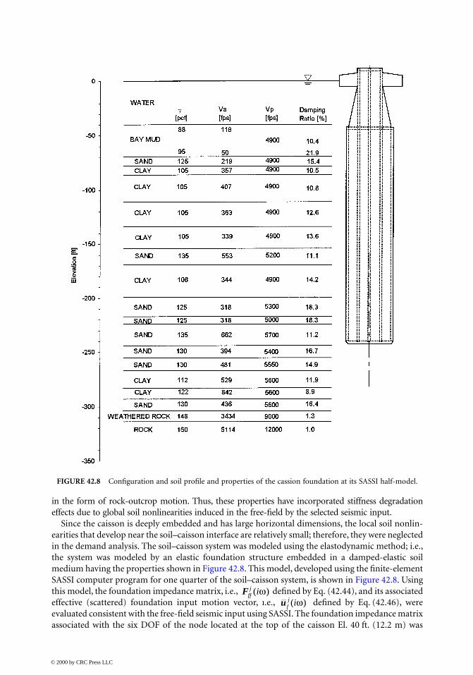
in the form of rock-outcrop motion. Thus, these properties have incorporated stiffness degradationeffects due to global soil nonlinearities induced in the free-field by the selected seismic input.
Since the caisson is deeply embedded and has large horizontal dimensions, the local soil nonlin-earities that develop near the soil–caisson interface are relatively small; therefore, they were neglectedin the demand analysis. The soil–caisson system was modeled using the elastodynamic method; i.e.,the system was modeled by an elastic foundation structure embedded in a damped-elastic soilmedium having the properties shown in Figure 42.8. This model, developed using the finite-elementSASSI computer program for one quarter of the soil–caisson system, is shown in Figure 42.8. Usingthis model, the foundation impedance matrix, i.e., defined by Eq. (42.44), and its associatedeffective (scattered) foundation input motion vector, i.e., defined by Eq. (42.46), wereevaluated consistent with the free-field seismic input using SASSI. The foundation impedance matrixassociated with the six DOF of the node located at the top of the caisson El. 40 ft. (12.2 m) was
FIGURE 42.8 Configuration and soil profile and properties of the cassion foundation at its SASSI half-model.
Fffj i( )ω
u fj i( )ω
© 2000 by CRC Press LLC
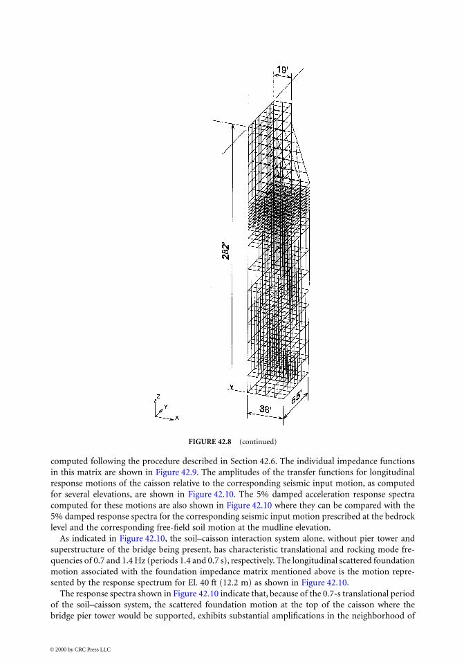
computed following the procedure described in Section 42.6. The individual impedance functionsin this matrix are shown in Figure 42.9. The amplitudes of the transfer functions for longitudinalresponse motions of the caisson relative to the corresponding seismic input motion, as computedfor several elevations, are shown in Figure 42.10. The 5% damped acceleration response spectracomputed for these motions are also shown in Figure 42.10 where they can be compared with the5% damped response spectra for the corresponding seismic input motion prescribed at the bedrocklevel and the corresponding free-field soil motion at the mudline elevation.
As indicated in Figure 42.10, the soil–caisson interaction system alone, without pier tower andsuperstructure of the bridge being present, has characteristic translational and rocking mode fre-quencies of 0.7 and 1.4 Hz (periods 1.4 and 0.7 s), respectively. The longitudinal scattered foundationmotion associated with the foundation impedance matrix mentioned above is the motion repre-sented by the response spectrum for El. 40 ft (12.2 m) as shown in Figure 42.10.
The response spectra shown in Figure 42.10 indicate that, because of the 0.7-s translational periodof the soil–caisson system, the scattered foundation motion at the top of the caisson where thebridge pier tower would be supported, exhibits substantial amplifications in the neighborhood of
FIGURE 42.8 (continued)
© 2000 by CRC Press LLC
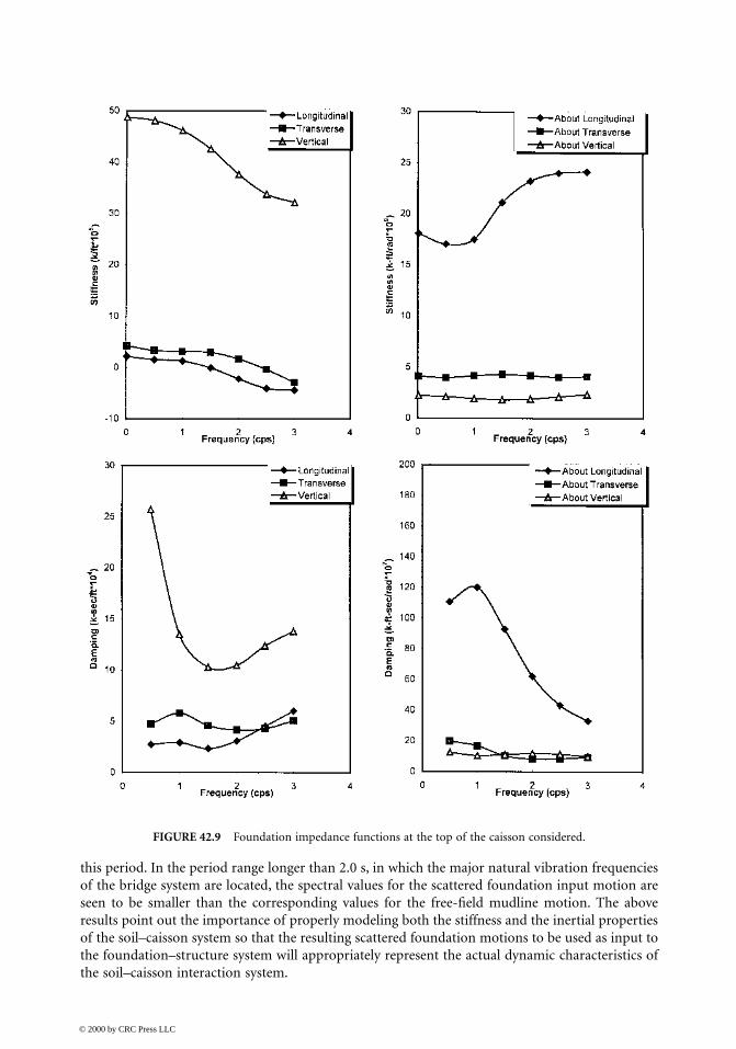
this period. In the period range longer than 2.0 s, in which the major natural vibration frequenciesof the bridge system are located, the spectral values for the scattered foundation input motion areseen to be smaller than the corresponding values for the free-field mudline motion. The aboveresults point out the importance of properly modeling both the stiffness and the inertial propertiesof the soil–caisson system so that the resulting scattered foundation motions to be used as input tothe foundation–structure system will appropriately represent the actual dynamic characteristics ofthe soil–caisson interaction system.
FIGURE 42.9 Foundation impedance functions at the top of the caisson considered.
© 2000 by CRC Press LLC
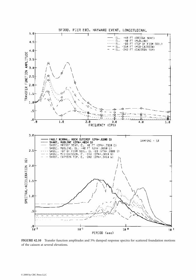
FIGURE 42.10 Transfer function amplitudes and 5% damped response spectra for scattered foundation motionsof the caisson at several elevations.
© 2000 by CRC Press LLC

42.7.2 Slender-Pile Group Foundation
The second example is to illustrate application of the empirical p–y method in a demand analysisof a slender-pile group foundation constructed at a deep soil site. The pile group foundation selectedis one of 78 pier foundations of a long, water-crossing steel truss bridge. The foundation is con-structed of two 24-ft (7.32-m)-diameter bell-shaped precast reinforced concrete pile caps, whichare linked together by a deep cross-beam, as shown in Figure 42.11. Each bell-shaped pile cap issupported on a group of 28 steel 14BP89 H-pipes, giving a total of 56 piles supporting the combinedtwo-bell pile cap. The piles in the outer ring and in the adjacent inner ring are battered at an angleof 4 to 1 and 6 to 1, respectively, leaving the remaining piles as vertical piles. The top ends of allpiles are embedded with sufficient lengths into the concrete that fills the interior space of the bell-shaped pile caps such that these piles can be considered as fixed-head piles. The piles penetrate deepinto the supporting soil medium to an average depth of 147 ft (44.8 m) below the mudline, wherethey encounter a thick dense sand layer. The soil profile and properties at this foundation locationare shown in Figure 42.12. As indicated in this figure, the top 55 ft (16.8 m) of the site soil iscomposed of a 35-ft (10.7-m) layer of soft bay mud overlying a 20-ft (6.1-m) layer of loose silty sand.
FIGURE 42.11 Configuration of the slender-pile group foundation considered.
© 2000 by CRC Press LLC
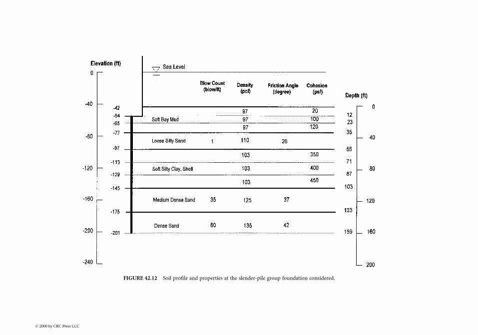
ndation considered.
© 2000
FIGURE 42.12 Soil profile and properties at the slender-pile group fou
by CRC Press LLC

Because of the soft topsoil layers and the slender piles used, the foundation under seismicexcitations is expected to undergo relatively large foundation lateral displacements relative to thefree-field soil. Thus, large local soil nonlinearities are expected to occur at the soil–pile interfaces.To model the nonlinear soil resistances to the lateral and axial deflections of the piles, the empiricallyderived lateral p–y and axial t–z, and the pile-tip Q–d curves for each pile were used. Typical p–yand t–z curves developed for the piles are shown in Figure 42.13. Using the nonlinear p–y, t–z, andQ–d curves developed, evaluation of the foundation impedance matrix, , and the associatedscattered foundation input motion vector, , were obtained following the proceduresdescribed below:
1. Determine the pile group deflected shape using a nonlinear analysis program such as GROUP[52], LPIPE [53], and APILE2 [54], as appropriate, under an applied set of monotonicallyincreasing axial and lateral forces and an overturning moment.
2. Select target levels of axial and lateral deflections at each selected soil depth correspondingto a selected target level of pile cap displacement and determine the corresponding secantmoduli from the applicable nonlinear p–y, t–z, and Q–d curves.
3. Develop a model of a group of elastic beams supported on elastic axial and lateral soil springsfor the pile group using the elastic properties of the piles and the secant moduli of the soilresistances obtained in Step 2 above.
4. Compute the foundation impedance matrix and associated scattered foundation inputmotion vector for the model developed in Step 3 using Eqs. (42.44) and (42.46).
Since the p–y, t–z, and Q–d curves represent pseudo-static force–deflection relations, the resultingfoundation impedance matrix computed by the above procedure is a real (not complex) frequency-independent pseudo-static stiffness matrix, i.e., . For the pile group foundationconsidered in this example, the beam-on-elastic-spring model shown schematically in Figure 42.14was used. The foundation stiffness matrix is associated with the six DOF of the nodal point locatedat the bottom center of the pile cap is shown in Figure 42.14. The scattered foundation motions inthe longitudinal, transverse, and vertical directions associated with this foundation stiffness matrixare represented by their 5% damped acceleration response spectra shown in Figure 42.15. Thesespectra can be compared with the corresponding spectra for the seismic input motion prescribedat the pile tip elevation and the free-field mudline motions computed from free-field site-responseanalyses using SHAKE. As shown in Figure 42.15, the spectral values for the scattered pile capmotions, which would be used as input to the foundation–structure system, are lower than thespectral values for the free-field mudline motions. This result is to be expected for two reasons: (1)the soft topsoil layers present at the site are not capable of driving the pile group foundation and(2) the battered piles, acting with the vertical piles, resist lateral loads primarily through stiff axialtruss action, in which case, the effective input motions at the pile cap are controlled more by thefree-field soil motions at depth, where more competent soil resistances are present, than by the soilmotions near the surface.
42.7.3 Large-Diameter Shaft Foundation
The third example illustrates the application of the demand analysis procedure using the hybridmethod of modeling. This method is preferred for a foundation constructed of a group of large-diameter CISS or CIDH shafts. Because of the large horizontal dimensions and substantial massesassociated with the shafts in this type of foundation, the dynamic interaction of the shafts with thesurrounding soil medium is more appropriately modeled and analyzed using the elastodynamicmethod; however, because the shafts resist loadings in a manner like piles, the local soil nonlinearitiespresent in the soil–shaft interface regions near the ground surface where soft soils are usually presentmay be sufficiently large that they should be explicitly considered using a method such as theempirical p–y method.
Ffff i( )ω
u f i( )ω
F Fffj
ffji( ) ( )ω = 0
© 2000 by CRC Press LLC

The foundation selected for this example is composed of two 10.5-ft (3.2 m)-diameter shafts150 ft (45.7 m) long, each consisting of a steel shell of wall thickness 1.375 in. (34.9 mm) filled withconcrete. These two shafts are designed to be used as seismic retrofit shear piles for adding lateralstiffnesses and lateral load-resistance capacities to the H-pile group foundation considered in thesecond example discussed previously. The two shafts are to be linked to the existing pile group at
FIGURE 42.13 Typical p–y and t–z curves for the piles of the slender-pile group foundation considered.
© 2000 by CRC Press LLC
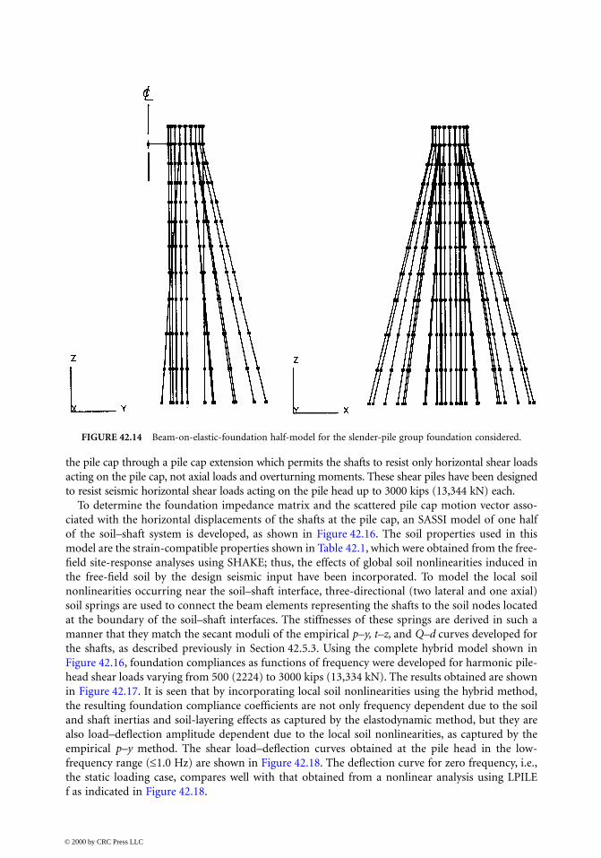
the pile cap through a pile cap extension which permits the shafts to resist only horizontal shear loadsacting on the pile cap, not axial loads and overturning moments. These shear piles have been designedto resist seismic horizontal shear loads acting on the pile head up to 3000 kips (13,344 kN) each.
To determine the foundation impedance matrix and the scattered pile cap motion vector asso-ciated with the horizontal displacements of the shafts at the pile cap, an SASSI model of one halfof the soil–shaft system is developed, as shown in Figure 42.16. The soil properties used in thismodel are the strain-compatible properties shown in Table 42.1, which were obtained from the free-field site-response analyses using SHAKE; thus, the effects of global soil nonlinearities induced inthe free-field soil by the design seismic input have been incorporated. To model the local soilnonlinearities occurring near the soil–shaft interface, three-directional (two lateral and one axial)soil springs are used to connect the beam elements representing the shafts to the soil nodes locatedat the boundary of the soil–shaft interfaces. The stiffnesses of these springs are derived in such amanner that they match the secant moduli of the empirical p–y, t–z, and Q–d curves developed forthe shafts, as described previously in Section 42.5.3. Using the complete hybrid model shown inFigure 42.16, foundation compliances as functions of frequency were developed for harmonic pile-head shear loads varying from 500 (2224) to 3000 kips (13,334 kN). The results obtained are shownin Figure 42.17. It is seen that by incorporating local soil nonlinearities using the hybrid method,the resulting foundation compliance coefficients are not only frequency dependent due to the soiland shaft inertias and soil-layering effects as captured by the elastodynamic method, but they arealso load–deflection amplitude dependent due to the local soil nonlinearities, as captured by theempirical p–y method. The shear load–deflection curves obtained at the pile head in the low-frequency range (≤1.0 Hz) are shown in Figure 42.18. The deflection curve for zero frequency, i.e.,the static loading case, compares well with that obtained from a nonlinear analysis using LPILEf as indicated in Figure 42.18.
FIGURE 42.14 Beam-on-elastic-foundation half-model for the slender-pile group foundation considered.
© 2000 by CRC Press LLC

Subjecting the foundation to the design seismic input motions prescribed at the pile tip elevationand the corresponding free-field soil motions over its full depth, scattered foundation motions inthe longitudinal and transverse directions of the bridge at the bottom center of the pile cap were
FIGURE 42.15 Comparisons of 5% damped response spectra for the rock input, mudline, and scattered pile capmotions in longitudinal, transverse, and vertical directions.
© 2000 by CRC Press LLC

obtained as shown in terms of their 5% damped acceleration response spectra in Figure 42.19, wherethey can be compared with the corresponding response spectra for the seismic input motions andthe free-field mudline motions. It is seen that, because of the substantial masses of the shafts, thespectral amplitudes of the scattered motions are higher than those of the free-field mudline motions
FIGURE 42.16 SASSI half-model of the large-diameter shaft foundation considered.
TABLE 42.1 Strain-Compatible Soil Properties for the Large-Diameter Shaft Foundation
Unit Wt., Shear Wave Compression Wave
El. ft (m)Depth; ft (m)
Thickness; ft (m)
Velocity Damping Ratio
Velocity, Damping Ratio
–50 (–15.2) 0 (0.0) 10 (3.05) 0.096 (15.1) 202.1 (61.6) 0.10 4,800 (1,463) 0.09–60 (–18.3) 10 (3.05) 10 (3.05) 0.096 (15.1) 207.5 (63.3) 0.15 5,000 (1,524) 0.10–70 (–21.3) 20 (6.10) 10 (3.05) 0.096 (15.1) 217.7 (66.4) 0.17 5,000 (1,524) 0.10–80 (–24.4) 30 (9.15) 20 (6.10) 0.110 (17.3) 137.5 (41.9) 0.25 4,300 (1,311) 0.10
–100 (–30.5) 50 (15.2) 10 (3.05) 0.096 (15.1) 215.7 (65.8) 0.20 4,800 (1,463) 0.10–110 (–33.5) 60 (18.3) 20 (6.10) 0.096 (15.1) 218.4 (66.6) 0.20 4,300 (1,311) 0.10–130 (–39.6) 80 (24.4) 20 (6.10) 0.096 (15.1) 233.0 (71.0) 0.20 4,900 (1,494) 0.10–150 (–45.7) 100 (30.5) 20 (6.10) 0.120 (18.8) 420.4 (128.2) 0.20 5,500 (1,677) 0.10–170 (–51.8) 120 (36.6) 10 (3.05) 0.120 (18.8) 501.0 (152.7) 0.19 6,000 (1,829) 0.10–180 (–54.9) 130 (39.6) 10 (3.05) 0.120 (18.8) 532.7 (162.4) 0.19 5,800 (1,768) 0.10–190 (–57.9) 140 (42.7) 20 (6.10) 0.125 (19.6) 607.2 (185.1) 0.18 5,800 (1,768) 0.10–210 (–64.0) 160 (48.8) 20 (6.10) 0.128 (20.1) 806.9 (246.0) 0.16 5,800 (1,768) 0.10–230 (–70.1) 180 (54.9) 10 (3.05) 0.133 (20.9) 1,374.4 (419.0) 0.11 6,400 (1,951) 0.10–240 (–78.2) 190 (57.9) 5 (1.52) 0.140 (21.9) 2,844.9 (867.3) 0.02 12,000 (3,658) 0.02–245 (–74.7) 195 (59.5) halfspace 0.145 (22.8) 6,387.2 (1,947.3) 0.01 12,000 (3,658) 0.01
kft
kNm3 3
fts
ms
fts
ms
© 2000 by CRC Press LLC
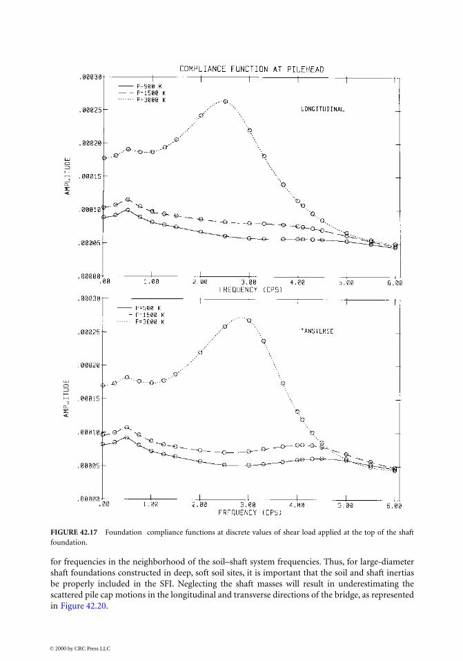
for frequencies in the neighborhood of the soil–shaft system frequencies. Thus, for large-diametershaft foundations constructed in deep, soft soil sites, it is important that the soil and shaft inertiasbe properly included in the SFI. Neglecting the shaft masses will result in underestimating thescattered pile cap motions in the longitudinal and transverse directions of the bridge, as representedin Figure 42.20.
FIGURE 42.17 Foundation compliance functions at discrete values of shear load applied at the top of the shaftfoundation.
© 2000 by CRC Press LLC
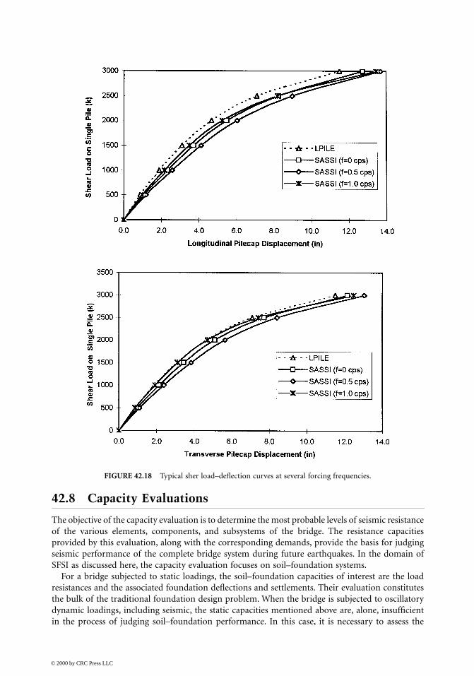
42.8 Capacity Evaluations
The objective of the capacity evaluation is to determine the most probable levels of seismic resistanceof the various elements, components, and subsystems of the bridge. The resistance capacitiesprovided by this evaluation, along with the corresponding demands, provide the basis for judgingseismic performance of the complete bridge system during future earthquakes. In the domain ofSFSI as discussed here, the capacity evaluation focuses on soil–foundation systems.
For a bridge subjected to static loadings, the soil–foundation capacities of interest are the loadresistances and the associated foundation deflections and settlements. Their evaluation constitutesthe bulk of the traditional foundation design problem. When the bridge is subjected to oscillatorydynamic loadings, including seismic, the static capacities mentioned above are, alone, insufficientin the process of judging soil–foundation performance. In this case, it is necessary to assess the
FIGURE 42.18 Typical sher load–deflection curves at several forcing frequencies.
© 2000 by CRC Press LLC

entire load–deflection relationships, including their cyclic energy dissipation characteristics, up toload and/or deformation limits approaching failure conditions in the soil–foundation system.Because of the complexity of this assessment, the capacity evaluation must be simplified in orderto make it practical. This is usually done by treating each soil–foundation system independentlyand by subjecting it to simplified pseudo-static monotonic and/or cyclic deformation-controlledstep-by-step patterns of loading, referred to here as “push-over” analysis.
FIGURE 42.19 Comparisons of 5% damped response spectra for the longitudinal and transverse rock input,mudline, and scattered pile cap motions for the shaft foundations at several shear load levels.
© 2000 by CRC Press LLC
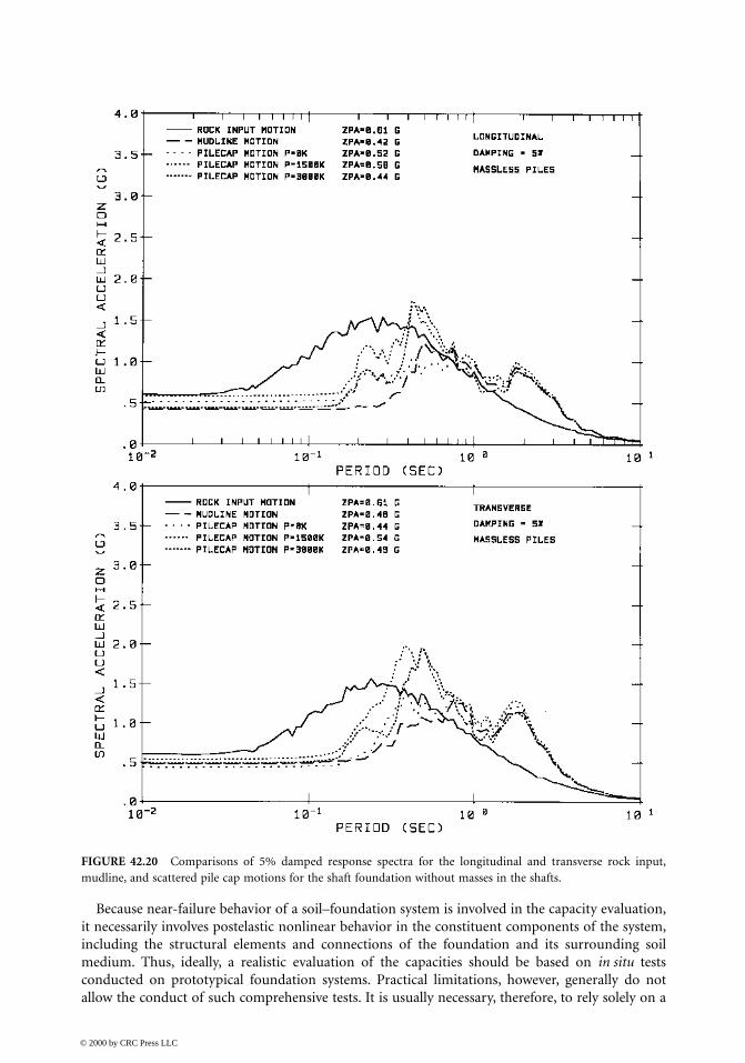
Because near-failure behavior of a soil–foundation system is involved in the capacity evaluation,it necessarily involves postelastic nonlinear behavior in the constituent components of the system,including the structural elements and connections of the foundation and its surrounding soilmedium. Thus, ideally, a realistic evaluation of the capacities should be based on in situ testsconducted on prototypical foundation systems. Practical limitations, however, generally do notallow the conduct of such comprehensive tests. It is usually necessary, therefore, to rely solely on a
FIGURE 42.20 Comparisons of 5% damped response spectra for the longitudinal and transverse rock input,mudline, and scattered pile cap motions for the shaft foundation without masses in the shafts.
© 2000 by CRC Press LLC

combination of analysis and limited-scope in situ or laboratory tests of selected critical components.These tests are performed either to provide the critical data needed for a capacity analysis or toconfirm the adequacy and reliability of the results obtained from such an analysis. Indicator-piletests that have often been performed for a bridge project are an example of limited-scope testing.
In a typical push-over analysis, the structural components of the foundation are represented byappropriate nonlinear finite elements capable of representing the near-failure nonlinear features,such as plastic hinging, ductile or brittle shearing, tensile or compressive yielding and fracturing,local and global buckling, and stiffness and capacity degradations due to P-∆ effects; further, thesurrounding soil medium is usually represented either by nonlinear finite elements capable ofmodeling the postelastic constitutive behavior of the material or by empirically derived generalizednonlinear soil springs such as those developed from the p–y, t–z, and Q–d curves used for pilefoundations. Ideally, the soil–foundation model used should also be able to represent properly theimportant nonlinear behaviors that could develop at the soil–foundation interfaces, such as slippage,debonding, and gapping. After the model has been developed, it is then subjected to a set of suitablepush-over loading programs that simulate the loading conditions imposed on the soil–foundationsystem by the bridge pier at its interface with the foundation.
Conducting a step-by-step push-over analysis of the model described above, one can identifyload and deformation levels associated with the various failure modes in the soil–foundation system.Then, load and deformation limits can be set beyond which the performance goals set for the bridgewill no longer be met. These limits can be considered the capacity limits of the foundation system.
Because large uncertainties usually exist in a capacity evaluation, the capacity limits obtainedtherefrom should be reduced using appropriate capacity reduction φ factors. Each reduction factoradopted should adequately cover the lower limit of capacity resulting from the uncertainties. Thereduced capacity limits established in this manner become the allowable capacity limits for use incomparing with the corresponding demands obtained through the demand analysis.
42.9 Concluding Statements
The previous sections of this chapter discuss the various elements of a modern state-of-the-art SFSIseismic analysis for large important bridges. These elements include (1) generating the site-specificrock-outcrop motions and corresponding free-field soil motions, (2) modeling and analysis ofindividual soil–foundation systems to establish foundation impedances and scattered motions, (3)determining SFSI using the substructuring method of analyses, and (4) assessing overall bridgeperformance by comparing force–deformation demands with corresponding capacities. Withoutretracing the details of these elements, certain points are worthy of special emphasis, as follows:
• Best-estimate rock and soil properties should be used in the generation of free-field seismicmotions, with full recognition of the variations (randomness) and uncertainties (lack ofknowledge) involved.
• Likewise, best-estimate material properties should be used in modeling the foundations, piers,abutments, and superstructure, also recognizing the variations and uncertainties involved.
• In view of the above-mentioned variations and uncertainties, sensitivity analyses should beconducted to provide a sound basis for judging overall seismic performance.
• Considering the current state of development, one should clearly differentiate between therequirements of a seismic force–deformation demand analysis and the corresponding capacityevaluation. The former is concerned with global system behavior; thus, it must satisfy onlyglobal dynamic equilibrium and compatibility. The latter, however, places emphasis on thebehavior of local elements, components, and subsystems, requiring that equilibrium andcompatibility be satisfied only at the local level within both the elastic and postelastic rangesof deformation.
© 2000 by CRC Press LLC
• In conducting a demand analysis, equivalent linear modeling, coupled with the substructuringmethod of analysis, has the advantages that (1) the results are more controllable and predict-able, (2) the uncertainties in system parameters can easily be evaluated separately, and (3)the SFSI responses can be assessed at stages. These advantages lead to a high level of confidencein the results when the nonlinearities are relatively weak. However, when strong nonlinearitiesare present, nonlinear time history analyses should be carried out in an iterative manner sothat system response is consistent with the nonlinearities.
• When strong nonlinearities are present in the overall structural system, usually in the piersand superstructure, multiple sets of seismic inputs should be used separately in conductingthe demand analyses; since, such nonlinearities cause relatively large dispersions of the max-imum values of critical response.
• The elastodynamic method of treating SFSI is valid for foundations having large horizontaldimensions, such as large spread footings and caissons; while the empirical p–y method isvalid only for slender-pile foundations subjected to large-amplitude deflections. For founda-tions intermediate between these two classes, e.g., those using large-diameter shafts, both ofthese methods are deficient in predicting SFSI behavior. In this case, the hybrid method ofmodeling has definitive advantages, including its ability to treat all classes of foundationswith reasonable validity.
• The p–y method of treating SFSI in both demand analyses and capacity evaluations needsfurther development, refinement, and validation through test results, particularly with regardto establishing realistic p–y, t–z, and Q–d curves. For seismic applications, changes in thecharacteristics of these curves, due to global soil nonlinearities induced by the free-fieldground motions, should be assessed.
• The hybrid method of treating SFSI, while being fundamentally sound, also needs furtherdevelopment, refinement, and test validation to make it fully acceptable for bridge applica-tions.
• Systematic research and development efforts, involving laboratory and field tests and analyt-ical correlation studies, are required to advance the SFSI analysis methodologies for treatingbridge foundations.
The state of the art of SFSI analysis of large bridge structures has been rapidly changing in recentyears, a trend that undoubtedly will continue on into the future. The reader is therefore encouragedto take note of new developments as they appear in future publications.
Acknowledgment
The authors wish to express their sincere thanks and appreciation to Joseph P. Nicoletti and AbbasAbghari for their contributions to Sections 42.2 and 42.4, respectively.
References
1. Mylonakis, G., Nikolaou, A., and Gazetas, G., Soil-pile-bridge seismic interaction: kinematic andinertia effects. Part I: Soft soil, Earthquake Eng. Struct. Dyn., 26, 337–359, 1997.
2. Tseng, W. S., Soil-foundation-structure interaction analysis by the elasto-dynamic method, in Proc.4th Caltrans Seismic Research Workshop, Sacramento, July 9–11, 1996.
3. Lam, I. P. and Law, H., Soil-foundation-structure interaction — analytical considerations by empir-ical p–y method, in Proc. 4th Caltrans Seismic Research Workshop, Sacramento, July 9–11, 1996.
4. Schnabel, P. B., Lysmer, J., and Seed, H. B., SHAKE — A Computer Program for EarthquakeResponse Analysis of Horizontally Layered Sites, Report No. EERC 72–12, Earthquake EngineeringResearch Center, University of California, Berkeley, 1972.
© 2000 by CRC Press LLC
5. Tseng, W. S. and Hadjian, A. H., Guidelines for Soil-Structure Interaction Analysis, EPRI NP-7395,Electric Power Research Institute, Palo Alto, CA, October 1991.
6. Richart, F. E., Hall, J. R., Jr., and Woods, R. D., Vibrations of Soils and Foundations, Prentice-Hall,Englewood Cliffs, NJ, 1970.
7. Veletsos, A. S. and Wei, Y. T., Lateral and rocking vibration of footings, J. Soil Mech. Found. Div.ASCE, 97(SM9), 1227–1249, 1971.
8. Kausel, E. and Roësset, J. M., Soil-structure interaction problems for nuclear containment struc-tures, in Proc. ASCE Power Division Specialty Conference, Denver, CO, August 1974.
9. Wong, H. L. and Luco, J. E., Dynamic response of rigid foundations of arbitrary shape, EarthquakeEng. Struct. Dyn., 4, 587–597, 1976.
10. Seed, H. B. and Idriss, I. M., Soil Moduli and Damping Factors for Dynamic Response Analysis,Report No. EERC 70-10, Earthquake Engineering Research Center, University of California, Ber-keley, 1970.
11. Waas, G., Analysis Method for Footing Vibrations through Layered Media, Ph.D. dissertation,University of California, Berkeley, 1972.
12. Lysmer, J., Udaka, T., Tsai, C. F., and Seed, H. B., FLUSH — A Computer Program for Approximate3-D Analysis of Soil-Structure Interaction, Report No. EERC75-30, Earthquake EngineeringResearch Center, University of California, Berkeley, 1975.
13. Tang, Y. K., Proceedings: EPRI/NRC/TPC Workshop on Seismic Soil-Structure Interaction AnalysisTechniques Using Data from Lotung Taiwan, EPRI NP-6154, Electric Power Research Institute,Palo Alto, CA, March 1989.
14. Matlock, H. and Reese, L. C., Foundation analysis of offshore pile supported structures, in Proc.5th Int. Conf. on Soil Mech. and Found. Eng., Paris, France, July 17–22, 1961.
15. Matlock, H., Correlations for design of laterally loaded piles in soft clay, in Proc. Offshore TechnologyConference, Paper No. OTC1204, Dallas, TX, April 22–24, 1970.
16. Reese, L. C., Cox, W. R., and Koop, F. D., Analysis of laterally loaded piles in sand, in Proc. OffshoreTechnology Conference, Paper No. OTC2080, Dallas, TX, May 6–8, 1974.
17. Chang, C. Y., Tseng, W. S., Tang, Y. K., and Power, M. S., Variations of earthquake ground motionswith depth and its effects on soil–structure interaction, Proc. Second Department of Energy NaturalPhenomena Hazards Mitigation Conference, Knoxville, Tennessee, October 3–5, 1989.
18. Abrahamson, N. A., Spatial Variation of Earthquake Ground Motion for Application to Soil-Structure Interaction, Report No. TR-100463, Electric Power Research Institute, Palo Alto, CA,March 1992.
19. Gasparini, D. and Vanmarcke, E. H., SIMQKE: A program for Artificial Motion Generation,Department of Civil Engineering, Massachusetts Institute of Technology, Cambridge, 1976.
20. Silva, W. J. and Lee, K., WES RASCAL Code for Synthesizing Earthquake Ground Motions, State-of-the-Art for Assessing Earthquake Hazards in United States, Report 24, Army Engineers WaterwayExperimental Station, Miscellaneous Paper 5-73-1, 1987.
21. Lilhanand, K. and Tseng, W. S., Development and application of realistic earthquake time historiescompatible with multiple-damping design response spectra, in Proc. 9th World Conference ofEarthquake Engineers, Tokyo-Kyoto, Japan, August 2–9, 1988.
22. Bolt, B. A. and Gregor, N. J., Synthesized Strong Ground Motions for the Seismic ConditionAssessment of Eastern Portion of the San Francisco Bay Bridge, Report No. EERC 93-12, EarthquakeEngineering Research Center, University of California, Berkeley, 1993.
23. Abrahamson, N. A., Nonstationary spectral matching, Seismol. Res. Lett., 63(1), 1992.24. Boore D. and Akinson, G., Stochastic prediction of ground motion and spectral response param-
eters at hard-rock sites in eastern North America, Bull. Seismol. Soc. Am., 77, 440–467, 1987.25. Sommerville, P. G. and Helmberger, D. V., Modeling earthquake ground motion at close distance,
in Proc. EPRI/Stanford/USGS Workshop on Modeling Earthquake Ground Motion at Close Distances,August 23, 1990.
© 2000 by CRC Press LLC

26. Papageorgiou, A. S. and Aki, K., A specific barrier model to the quantitative description of inho-mogeneous faulting and the prediction of strong motion, Bull. Seismol. Soc. Am., Vol. 73, 693–722,953–978, 1983.
27. Bolt, B. A., Ed., Seismic Strong Motion Synthetics, Academic Press, New York, 1987.28. U.S. Nuclear Regulatory Commission, Standard Review Plan, Section 3.71., Revision 2, Washington,
D.C., August, 1989.29. International Conference of Building Officials, Uniform Building Code, Whittier, CA, 1994.30. Kaul, M. K., Spectrum-consistent time-history generation, J. Eng. Mech. Div. ASCE, 104(EM4),
781, 1978.31. Penzien, J. and Watabe, M., Simulation of 3-dimensional earthquake ground motions, J. Earthquake
Eng. Struct. Dyn., 3(4), 1975.32. Hao, H., Oliviera, C. S., and Penzien, J., Multiple-station ground motion processing and simulation
based on SMART-1 array data, Nuc. Eng. Des., III(6), 2229–2244, 1989.33. Chang, C. Y., Power, M. S., Idriss, I. M., Sommerville, P. G., Silva, W., and Chen, P. C., Engineering
Characterization of Ground Motion, Task II: Observation Data on Spatial Variations of EarthquakeGround Motion, NUREG/CR-3805, Vol. 3, U.S. Nuclear Regulatory Commission, Washington,D.C., 1986.
34. Abrahamson, N. A., Schneider, J. F., and Stepp, J. C., Empirical spatial coherency functions forapplication to soil-structure interaction analyses, Earthquake Spectra, 7, 1, 1991.
35. Tseng, W. S., Lilhanand, K., and Yang, M. S., Generation of multiple-station response-spectra-and-coherency-compatible earthquake ground motions for engineering applications, in Proc. 12th Int.Conference on Struct. Mech. in Reactor Technology, Paper No. K01/3, Stuttgart, Germany, August15–20, 1993.
36. Vucetic, M. and Dobry, R., Effects of soil plasticity on cyclic response, J. Geotech. Eng. ASCE, 117(1),89–107, 1991.
37. Sun, J. I., Golesorkhi, R., and Seed, H. B., Dynamic Moduli and Damping Ratios for Cohesive Soils,Report No. UBC/EERC-88/15, Earthquake Engineer Research Center, University of California,Berkeley, 1988.
38. Hardin, B. O. and Drnevich, V., Shear modulus and damping in soils: design equations and curves,J. Soil Mech. Found. Div. ASCE, 98(7), 667–691, 1972.
39. Seed, H. B., and Idriss, I. M., Soil Moduli and Damping Factors for Dynamic Response Analyses,Report No. EERC 70-10, Earthquake Engineering Research Center, University of California,Berkeley, 1970.
40. Seed, H. B., Wong, R. T., Idriss, I. M., and Tokimatsu, K., Moduli and Damping Factors forDynamic Analyses of Cohesionless Soils, Report No. UCB/EERC-84/14, Earthquake EngineeringResearch Center, University of California, Berkeley, 1984.
41. Hardin, B. O. and Black, W. L., Vibration modulus of normally consolidated clay, J. Soil Mech.Found. Div. ASCE, 94(2), 353–369, 1968.
42. Hardin, B. O., The nature of stress-strain behavior for soils, Proc. ASEC Geotech. Eng. Div. SpecialtyConference on Earthquake Eng. and Soil Dyn., Vol. 1, 3-90, 1978.
43. Dickenson, S. E., Dynamic Response of Soft and Deep Cohesive Soils During the Loma Prietaearthquake of October 17, 1989, Ph.D. dissertation, University of California, Berkeley, 1994.
44. Idriss, I. M. and Sun, J. I., User’s Manual for SHAKE 91, Center for Geotechnical Modeling,University of California, Davis, 1992.
45. Seed, H. B. and Idriss, I. M., Influence of soil conditions on ground motions during earthquakes,J. Soil Mech. Found. Div., 95(SM1), 99–138, 1969.
46. Lee, M. K. W. and Finn, W. D. L., DESRA-2: Dynamic Effective Stress Response Analysis of SoilDeposits with Energy Transmitting Boundary Including Assessment of Liquification Potential,Report No. 38, Soil Mechanics Series, Department of Civil Engineering, University of BritishColumbia, Vancouver, 1978.
© 2000 by CRC Press LLC
47. Prevost, J. H. DYNAFLOW: A Nonlinear Transient Finite Element Analysis Program, Departmentof Civil Engineering and Operations Research, Princeton University, Princeton, NJ, 1981; lastupdate, 1993.
48. Prevost, J. H., DYNAID: A Computer Program for Nonlinear Seismic Site Response Analysis,Report No. NCEER-89-0025, National Center for Earthquake Engineering Research, Buffalo, NewYork, 1989.
49. Li, X. S., Wang, Z. L., and Shen, C. K., SUMDES, A Nonlinear Procedure for Response Analysis ofHorizontally-Layered Sites, Subjected to Multi-directional Earthquake Loading, Department ofCivil Engineering, University of California, Davis, 1992.
50. Apsel, R. J., Dynamic Green’s Function for Layered Media and Applications to Boundary ValueProblems, Ph.D. thesis, University of California, San Diego, 1979.
51. Lysmer, J., Tabatabaie-Raissai, M., Tajirian, F., Vahdani, S., and Ostadan, F., SASSI — A System forAnalysis of Soil-Structure Interaction, Report No. UCB/GT/81-02, Department of Civil Engineer-ing, University of California, Berkeley, 1981.
52. Reese, L. C., Awoshirka, K., Lam, P. H. F., and Wang, S. T., Documentation of Computer ProgramGROUP — Analysis of a Group of Piles Subjected to Axial and Lateral Loading, Ensoft, Inc., Austin,TX, 1990.
53. Reese, L. C. and Wang, S. T., Documentation of Computer Program LPILE — A Program forAnalysis of Piles and Drilled Shafts under Lateral Loads,” Ensoft, Inc., Austin, TX, 1989; latestupdate, Version 3.0, May 1997.
54. Reese, L. C. and Wang, S. T., Documentation of Computer Program APILE2 — Analysis of LoadVs. Settlement for an Axially Loaded Deep Foundation, Ensoft, Inc., Austin, TX, 1990.
55. Seed, H. B. and Idriss, I. M., Rock Motion Accelerograms for High-Magnitude Earthquakes, ReportNo. EERC 69-7, Earthquake Engineering Research Center, University of California, Berkeley, 1969.
56. Clough, R. W. and Penzien, J., Dynamics of Structures, 2nd ed., McGraw-Hill, New York, 1993.
© 2000 by CRC Press LLC


![Structure] SAP2000 Dynamics of Structures -3rd Edition[Ray W.clough][Joseph Penzien]](https://static.fdocuments.us/doc/165x107/5478d723b4af9f47558b461d/structure-sap2000-dynamics-of-structures-3rd-editionray-wcloughjoseph-penzien.jpg)