Atmos. Chem. Phys., 12, 5897–5912, 2012www.atmos-chem-phys.net/12/5897/2012/doi:10.5194/acp-12-5897-2012© Author(s) 2012. CC Attribution 3.0 License.

AtmosphericChemistry

and Physics

Tropospheric methanol observations from space: retrievalevaluation and constraints on the seasonality of biogenic emissions

K. C. Wells1, D. B. Millet 1, L. Hu1, K. E. Cady-Pereira2, Y. Xiao2, M. W. Shephard3,*, C. L. Clerbaux4,5, L. Clarisse5,P.-F. Coheur5, E. C. Apel6, J. de Gouw7,8, C. Warneke7,8, H. B. Singh9, A. H. Goldstein10, and B. C. Sive11

1Department of Soil, Water and Climate, University of Minnesota, St. Paul, Minnesota, USA2Atmospheric and Environmental Research, Inc., Lexington, Massachusetts, USA3Environment Canada, Downsview, Ontario, Canada4UMPC Univ. Paris 06, Universite Versailles St-Quentin, CNRS/INSU, LATMOS-IPSL, Paris, France5Spectroscopie de l’Atmosphere, Service de Chimie Quantique et Photophysique, Universite Libre de Bruxelles, Brussels,Belgium6Atmospheric Chemistry Division, NCAR, Boulder, Colorado, USA7Earth System Research Laboratory, NOAA, Boulder, Colorado, USA8CIRES, University of Colorado, Boulder, Colorado, USA9NASA Ames Research Center, Moffett Field, California, USA10Departments of Environmental Science, Policy, and Management and of Civil and Environmental Engineering, UCBerkeley, Berkeley, California, USA11Department of Chemistry, Appalachian State University, Boone, North Carolina, USA* presently at: Atmospheric and Climate Applications (ACApps), Inc., East Gwillimbury, Ontario, Canada

Correspondence to:D. B. Millet (dbm@umn.edu)

Received: 16 December 2011 – Published in Atmos. Chem. Phys. Discuss.: 3 February 2012Revised: 12 June 2012 – Accepted: 13 June 2012 – Published: 12 July 2012

Abstract. Methanol retrievals from nadir-viewing space-based sensors offer powerful new information for quanti-fying methanol emissions on a global scale. Here we ap-ply an ensemble of aircraft observations over North Amer-ica to evaluate new methanol measurements from the Tropo-spheric Emission Spectrometer (TES) on the Aura satellite,and combine the TES data with observations from the In-frared Atmospheric Sounding Interferometer (IASI) on theMetOp-A satellite to investigate the seasonality of methanolemissions from northern midlatitude ecosystems. Using theGEOS-Chem chemical transport model as an intercompari-son platform, we find that the TES retrieval performs wellwhen the degrees of freedom for signal (DOFS) are above0.5, in which case the model:TES regressions are generallyconsistent with the model:aircraft comparisons. Including re-trievals with DOFS below 0.5 degrades the comparisons, asthese are excessively influenced by the a priori. The compar-isons suggest DOFS>0.5 as a minimum threshold for in-terpreting retrievals of trace gases with a weak tropospheric

signal. We analyze one full year of satellite observationsand find that GEOS-Chem, driven with MEGANv2.1 bio-genic emissions, underestimates observed methanol concen-trations throughout the midlatitudes in springtime, with thetiming of the seasonal peak in model emissions 1–2 monthstoo late. We attribute this discrepancy to an underestimate ofemissions from new leaves in MEGAN, and apply the satel-lite data to better quantify the seasonal change in methanolemissions for midlatitude ecosystems. The derived parame-ters (relative emission factors of 11.0, 0.26, 0.12 and 3.0 fornew, growing, mature, and old leaves, respectively, plus a leafarea index activity factor of 0.5 for expanding canopies withleaf area index<1.2) provide a more realistic simulation ofseasonal methanol concentrations in midlatitudes on the ba-sis of both the IASI and TES measurements.

Published by Copernicus Publications on behalf of the European Geosciences Union.

5898 K. C. Wells et al.: Tropospheric methanol observations from space

1 Introduction

Methanol (CH3OH) is the most abundant non-methanevolatile organic compound (VOC) in the atmosphere, witha global burden of 3–4 Tg, and is an important precursor ofCO, HCHO, and O3 (Tie et al., 2003; Millet et al., 2006;Duncan et al., 2007; Choi et al., 2010; Hu et al., 2011). Themajor source of atmospheric methanol is terrestrial plants;plants emit methanol primarily during cell growth (Macdon-ald and Fall, 1993; Nemecek-Marshall et al., 1995; Galballyand Kirstine, 2002; Karl et al., 2003; Harley et al., 2007) and,to a lesser extent, during decay (Warneke et al., 1999; Karlet al., 2005). Because long-term observations of atmosphericmethanol are limited, the spatial distribution, strength, andseasonality of these biogenic emissions are not currently wellconstrained. Here we use aircraft measurements and a globalchemical transport model (GEOS-Chem CTM) to evaluatenew space-based observations of tropospheric methanol, andinterpret the satellite data in terms of their constraints on theseasonality of biogenic methanol emission fluxes.

Current estimates of the total source of methanol to theatmosphere range from 122 to 350 Tg yr−1 (Heikes et al.,2002; Tie et al., 2003; Singh et al., 2004; Jacob et al., 2005;Millet et al., 2008). Along with emissions from terrestrialplants, sources include atmospheric production via methaneoxidation (Tyndall et al., 2001), burning of biomass and bio-fuels (Holzinger et al., 1999; Andreae and Merlet, 2001), andurban/industrial emissions (Holzinger et al., 2001; de Gouwet al., 2005; Hu et al., 2011). Gross emissions from marinebiota are estimated to be comparable in magnitude to thosefrom terrestrial plants (Millet et al., 2008); however, oceansare an overall net sink of atmospheric methanol (Heikes etal., 2002; Carpenter et al., 2004; Williams et al., 2004; Milletet al., 2008; Stavrakou et al., 2011). The other major removalmechanism for methanol is photochemical oxidation by OH,with deposition to land surfaces also being significant (Ja-cob et al., 2005; Karl et al., 2010). Estimates of the atmo-spheric lifetime of methanol range from 5–12 days (Galballyand Kirstine, 2002; Tie et al., 2003; Jacob et al., 2005).

Recent modeling studies have found that current emissioninventories give rise to substantial regional biases in pre-dicted versus measured methanol concentrations. Millet etal. (2008) compared methanol concentrations simulated byGEOS-Chem (using a net primary production (NPP)-basedapproach for estimating biogenic emissions) to available air-craft and ground-based measurements, and found evidencefor a ∼50 % overestimate of biogenic methanol emissionsin the eastern US and the Amazon from broadleaf treesand crops. More recently, Stavrakou et al. (2011) employeddata from the Infrared Atmospheric Sounding Interferome-ter (IASI) satellite sensor to constrain biogenic and biomassburning emissions of methanol. Using a different biogenicemission scheme (MEGAN) and the IMAGESv2 CTM, theyfound a similar overestimate of methanol emissions frombroadleaf trees in the eastern US, Amazonia, and Indonesia;

however, their results also revealed an underestimate of thebiogenic source in more arid regions such as central Asia(by up to a factor of five) and the western US (by a factorof two). Hu et al. (2011) compared methanol measurementsfrom a tall tower in the US Upper Midwest to predicted con-centrations from GEOS-Chem driven by MEGAN biogenicemissions. The model-measurement comparisons indicateda modest underestimate (∼35 %) of methanol emissions forthat region in summer, but also revealed a significant bias inthe seasonality of the modeled biogenic source. This biasedmodel seasonality led to an underestimate of the photochem-ical role for methanol early in the growing season.

New methanol retrievals from nadir-viewing space-bornesensors offer key information for quantifying biogenicmethanol sources to the atmosphere and the correspondingimpacts on tropospheric chemistry. In this paper, we use air-craft measurements from an ensemble of field campaigns(Intercontinental Transport Experiment-Phase B, INTEX-B; Megacity Initiative: Local and Global Research Obser-vations, MILAGRO; the second Texas Air Quality Study,TexAQS-II; Arctic Research of the Composition of the Tro-posphere from Aircraft and Satellites, ARCTAS; Aerosol,Radiation, and Cloud Processes affecting Arctic Climate,ARCPAC) with the GEOS-Chem CTM to (i) evaluate at-mospheric methanol retrievals from the Tropospheric Emis-sion Spectrometer (TES), and (ii) interpret the TES and IASIspace-borne observations in terms of the seasonality of bio-genic emissions from major plant functional types in midlat-itude ecosystems.

2 Methanol measurements from space

Atmospheric methanol was first detected from space via so-lar occultation spectra from the Atmospheric Chemistry Ex-periment infrared Fourier Transform Spectrometer (ACE-FTS), a limb-viewing infrared sounder onboard the SCISAT-1 satellite (Bernath et al., 2005). Enhanced concentrationsof methanol were retrieved in the upper troposphere/lowerstratosphere in the vicinity of biomass burning plumes (Du-four et al., 2006); subsequent analysis of several years ofACE retrievals showed that a majority of the upper tropo-spheric methanol burden in the Northern Hemisphere is bio-genic in origin (Dufour et al., 2007). The ACE measurementsprovide important data for determining the influence of sur-face emissions on upper tropospheric composition, but dueto lack of sensitivity in the lower atmosphere they providelimited information on the sources themselves.

Two nadir-viewing infrared sounders currently in spaceprovide observations of methanol in the lower troposphere:TES, launched onboard the EOS Aura satellite in July 2004(Beer et al., 2001), and IASI, launched onboard the MetOp-A satellite in October 2006 (Clerbaux et al., 2009). We usedata from both of these sensors in this work.

Atmos. Chem. Phys., 12, 5897–5912, 2012 www.atmos-chem-phys.net/12/5897/2012/

K. C. Wells et al.: Tropospheric methanol observations from space 5899

2.1 TES methanol retrieval

TES, onboard EOS Aura in a polar sun-synchronous orbit(equator overpass 1345 local standard time), is an infraredFourier transform spectrometer with a spectral resolution of0.06 cm−1 (apodized) and 5×8 km2 footprint at nadir. Pro-files of species such as O3, CO2, CH4, H2O and HDO (mon-odeuterated water vapor) are derived from the nadir measure-ments as standard products. The TES retrieval uses an opti-mal estimation approach, allowing the averaging kernels anderror estimates to be directly determined as a part of the re-trieval (Rodgers, 2000). The first observations of methanolfrom TES were reported in Beer et al. (2008). These firstresults showed high concentrations in the Beijing area, anddemonstrated the ability of the sensor to detect localized ur-ban methanol enhancements. Xiao et al. (2012) also recentlydemonstrated the ability of TES to detect methanol enhance-ments in Mexico City outflow.

The atmospheric methanol abundance is retrieved basedon the spectral residuals between the TES measurements anda forward radiative transfer model (Clough et al., 2006) from1032.32 to 1034.48 cm−1. This spectral range encompassestheν8 C-O stretching band, which is the strongest absorptionband for methanol. An example TES observation over NorthAmerica is shown in Fig. 1 (top panel). The data have unitsof brightness temperature, i.e. the temperature a blackbodywould need to achieve to emit radiation at the observed inten-sity. The second panel shows the difference between the ob-served spectrum and a modeled spectrum computed assum-ing a methanol-free atmosphere, while the third panel showsthe measurement-model difference after three iterations tooptimize the methanol profile in the forward model. The dif-ference between the model spectrum without methanol andthat with methanol is shown in the fourth panel, illustratingthe brightness temperature signal (∼1 K) for methanol in thisexample.

A detailed description of the TES retrieval strategy, ini-tial performance, and sensitivity is provided by Cady-Pereiraet al. (2012). The a priori methanol profiles in the TES re-trievals are based on simulated profiles for the year 2004from the GEOS-Chem CTM (described in Sect. 3). Four apriori profiles are employed, corresponding to clean marine,enhanced marine, clean continental and enhanced continentalscenes. The clean marine profile was obtained by averagingall simulated marine profiles with mixing ratios≤1 ppb be-low 500 hPa, while the clean continental profile was obtainedby averaging all simulated continental profiles with surfacemixing ratios≤2 ppb. The enhanced marine and continen-tal profiles were derived by averaging the model profiles thatexceeded these respective thresholds.

The retrieved methanol profilex is related to the true pro-file x by

x = xa+ A(x − xa) (1)

Fig. 1. An example TES methanol retrieval from 7 July 2008(54.45◦ N, 113.05◦ W). (A) Spectral brightness temperature ob-served by TES.(B) Residuals between the TES measured spectrumand a modeled spectrum computed assuming a methanol-free atmo-sphere.(C) Measurement-model residuals after three iterations ofthe forward model to optimize the methanol profile.(D) Differencebetween the second and third panels, showing the brightness tem-perature signal associated with methanol. In each case the spectralrange used for the retrieval is shown in red.(E) The correspondingretrieved methanol profile (black line), a priori profile (red line),and the representative volume mixing ratio (RVMR, black symbol)for this example. The shaded bar indicates the vertical range overwhich the RVMR applies, corresponding to the full width at half-maximum of the averaging kernel peak.(F) The sum of rows of theaveraging kernel for this example.

wherexa is the a priori profile andA is the averaging kernelmatrix. The a priori used in the above example correspondsto an enhanced continental profile, and is shown in the lowerleft panel of Fig. 1 along with the retrieved profile.

A series of simulated retrievals based on perturbed TESprofiles was used to test the performance of the methanolretrieval algorithm. The results, described in detail by Cady-Pereira et al. (2012), show that the retrieval has low meanbias (0.16 ppb at 825 hPa), with a standard deviation of0.34 ppb. The sum of the rows of the averaging kernel ma-trix (shown for the above example in the lower right panel ofFig. 1) indicates the fraction of information coming from themeasurement versus the a priori. In the example of Fig. 1,we see that peak sensitivity to the atmospheric state occurs

www.atmos-chem-phys.net/12/5897/2012/ Atmos. Chem. Phys., 12, 5897–5912, 2012

5900 K. C. Wells et al.: Tropospheric methanol observations from space

at ∼800 hPa. The TES methanol retrievals most commonlyexhibit peak sensitivity between∼700 and 900 hPa; aboveand below this vertical range, most of the information comesfrom the a priori.

The degrees-of-freedom for signal (DOFS) reflect the in-formation content of the retrieval (i.e. the number of inde-pendent variables that can be determined from the measure-ment), and are calculated as the trace of the averaging ker-nel matrix. Since the methanol spectral signature in nadirinfrared observations is relatively weak (DOFS generally<1.0), limited information about the true vertical profile canbe obtained from the TES measurements. Therefore, in thefollowing analyses we transform the retrieved profile into asingle Representative Volume Mixing Ratio, RVMR (Payneet al., 2009; Shephard et al., 2011). The RVMR,ρ, provides ameasure of the methanol amount at the vertical level(s) wherethe retrieval is most sensitive.

For methanol, the RVMR is calculated from the retrievedprofile as follows:

ρ = exp

[nlevs∑i=1

log(wi xi)

](2)

wherexi is the retrieved mixing ratio at leveli, andwi is theRVMR weighting function at leveli. The RVMR weightingfunction is derived from a transformation of the averagingkernel matrix; when the total amount of retrieved informa-tion is limited (DOFS≤1.0), as is the case for methanol, itreduces to a vector. The RVMR applies to the pressure rangespanned by the full width at half-maximum of the averagingkernel peak, and for the above retrieval example is 5.6 ppb(Fig. 1). RVMR values typically have an uncertainty from 10to 50 %, with the higher relative uncertainties correspondingto smaller RVMR values.

To compare TES retrievals with GEOS-Chem model out-put, we sample the model at the location and time of thesatellite overpass, and apply the corresponding TES a prioriprofile and averaging kernel using Eq. (1) to derive a modelprofile as it would be detected by TES. We then calculatethe model RVMR based on Eq. (2). For this work, retrievalsare performed only for cloud optical depths<1.0, and subse-quent to the retrieval of surface temperature and emissivity,water vapor, O3, and temperature profiles.

2.2 IASI methanol retrieval

IASI, onboard the MetOp-A satellite in a polar sun-synchronous orbit (equator overpass 0930 local standardtime), is an infrared Fourier transform spectrometer with aspectral resolution of 0.5 cm−1 (apodized) and a 12 km foot-print diameter at nadir. Given the wide swath (2200 km) ofthe instrument’s scans, IASI achieves global coverage twicedaily, resulting in over 1 000 000 measured spectra each day.IASI spectra were first used to retrieve methanol in biomassburning plumes (Coheur et al., 2009), and were found to have

sufficient temporal and spatial resolution to track the loss ofmethanol during plume aging.

Retrieval details and global results were recently reportedby Razavi et al. (2011). To make use of the high volumeof data provided by IASI, the global methanol retrieval usesa fast brightness temperature difference method. In this ap-proach, the difference in brightness temperature between themethanol absorption band (981.25 to 1038 cm−1) and base-line channels with minimal methanol absorption is calcu-lated, and that difference is converted to a total methanolcolumn using a conversion factor. One oceanic and one con-tinental conversion factor are used; these conversion factorswere developed using a subset of full optimal estimation re-trievals at select locations around the globe. Average oceanicand continental profiles of methanol from the IMAGESv2global CTM (Stavrakou et al., 2009, 2011) provide a prioriinformation for the retrieval. Only pixels with<2 % cloudcover are used. The uncertainty estimate for the retrievedmethanol column is±50 %. The mean averaging kernel fromthe optimal estimation retrievals indicates that IASI’s sen-sitivity to methanol peaks between∼5 and 10 km elevationover land.

3 GEOS-Chem methanol simulation

We use the GEOS-Chem global 3-D CTM version 8.3.1(http://www.geos-chem.org) as an intercomparison platformfor evaluating the satellite data against aircraft measure-ments, and to interpret the TES and IASI data in terms ofmethanol emission processes. GEOS-Chem uses GEOS-5 as-similated meteorological data from the NASA Goddard EarthObserving System, which have a resolution of 0.5◦

×0.667◦

with 72 vertical levels. We degrade these to a resolution of2◦

×2.5◦ with 47 vertical levels for our simulations, and usea one-year spin-up to remove the effect of initial conditions.The sources and sinks of atmospheric methanol are mod-eled using the simulation described by Millet et al. (2008),with the emission updates described below. Anthropogenicmethanol emissions are estimated from those of CO based ona methanol:CO emission ratio of 0.012 mol mol−1 (Goldanet al., 1995; de Gouw et al., 2005; Millet et al., 2005;Warneke et al., 2007). Global anthropogenic CO emissionsare from the GEIA inventory (www.geiacenter.org) over-written with the following regional inventories: EPA/NEI99emissions over the US (modified to account for recent COand NOx reductions; Hudman et al., 2007; 2008); Streets-2006 over Asia (Zhang et al., 2009); BRAVO over Mex-ico (Kuhns et al., 2003); EMEP over Europe (Vestreng andKlein, 2002; Auvray and Bey, 2005); and NPRI over Canada(http://www.ec.gc.ca/inrp-npri). Biomass burning emissionsare derived from the monthly GFEDv2 database (van derWerf et al., 2006) using a methanol:CO emission ratioof 0.018 mol mol−1 (Andreae and Merlet, 2001). GFEDv2

Atmos. Chem. Phys., 12, 5897–5912, 2012 www.atmos-chem-phys.net/12/5897/2012/

K. C. Wells et al.: Tropospheric methanol observations from space 5901

extends through 2008; biomass burning emissions for lateryears are set to the 2008 values.

Terrestrial biogenic emissions of methanol are computedusing the Model of Emissions of Gases and Aerosols fromNature (MEGANv2.1) (Guenther et al., 2006; Stavrakou etal., 2011). Emissions within a GEOS-Chem grid box areestimated as the sum of contributions from five plant func-tional types (PFTs: broadleaf trees, needleleaf trees, shrubs,grasses, and crops):

E = γ

5∑i=1

εiχi (3)

whereεi is the canopy emission factor at standard condi-tions for PFTi , χ i is the fractional grid box coverage ofPFTi , andγ is an activity factor used to scale the emissionsto local environmental conditions. The total activity factoris derived from individual activity factors for photosynthet-ically active radiation (PAR), temperature (T ), leaf area in-dex (LAI), and leaf age, each equal to 1.0 under standardconditions (PAR = 1500 µmol m−2 s−1; T = 303 K; LAI = 5;leaf age fractions of 0 % new leaves, 10 % growing leaves,80 % mature leaves, 10 % old leaves). The modeled temper-ature dependence treats the light-independent fraction (LIF)and light-dependent fraction (LDF) of emissions separately:

γ = γageγLAI[(1− LDF)γT ,LIF + (LDF)γPARγT ,LDF

](4)

with LDF = 0.8. Light-independent emissions are scaled byγ T ,LIF = exp(β(T − 303)), whereT is surface temperature(K) and β is the temperature response factor (0.08). Forγ T ,LDF, MEGANv2.1 uses the relationship defined for iso-prene (Guenther et al., 2006) with coefficients as reported inStavrakou et al. (2011). The PAR and LAI activity factors arecalculated using the PCEEA algorithm, which is described inGuenther et al. (2006).

Canopy emission factorsεi are set to 800 µg m−2 h−1 forneedleleaf trees, shrubs, crops, and non-tropical broadleaftrees, and 400µg m−2 h−1 for grasses and tropical broadleaftrees. The fractional coverage of each PFT is based onMEGAN landcover data (PFTv2.0), which is derived froma combination of satellite data, ground survey information,and the Olson et al. (2001) ecosystem database. For localLAI data we use climatological monthly-mean values fromMODIS Collection 5 (Yang et al., 2006), which are parti-tioned into leaf age classes (new, growing, mature, old) usingthe method outlined in Guenther et al. (2006). The fraction ofeach leaf age class,F , is used to calculate the activity factorfor leaf age as:

γage= FnewAnew+ FgrowingAgrowing+ FmatureAmature+ FoldAold (5)

whereA is the relative methanol emission rate for each leafage class. MEGANv2.1 uses relative emission rates of 3.0,2.6, 0.85, and 1.0 for new, growing, mature, and old leaves,respectively. A key objective of this work will be to derive

a more robust constraint on these parameters using satellitedata.

We performed global simulations for the years 2006–2009 to coincide with periods of available in situ and satel-lite observations (see Sect. 4). The total global methanolsource in our simulations is∼200 Tg yr−1. The global terres-trial biogenic methanol source is approximately∼66 Tg yr−1

with little interannual variability (source and sink magni-tudes are listed in Table S1 in the Supplement). The bio-genic source is lower than the recent optimized estimatesof Stavrakou (2011) and Millet (2008) by about 30 %.Stavrakou et al. (2011) employed a different canopy modeland meteorological fields than used here, while Millet etal. (2008) employed an NPP-based approach (rather than theMEGAN model) to estimate biogenic emissions.

4 Model-observation comparison over North America

We use in situ data from recent North American aircraft cam-paigns to evaluate the space-borne methanol retrievals: MI-LAGRO (Singh et al., 2009; Kleb et al., 2011) over Mex-ico, the Gulf of Mexico, and southern Texas (March 2006);INTEX-B (Singh et al., 2009; Kleb et al., 2011) over thePacific Ocean and western US (April/May 2006); ARCPAC(Brock et al., 2011) over the US (transit flight to Alaska,April 2008); ARCTAS (Jacob et al., 2010) over Canada andthe western US (June/July 2008, which comprised the lat-ter phase of the study); and TexAQS-II (Parrish et al., 2009)over the Houston area (September/October 2006). Measure-ment techniques for each campaign are listed in Table 1, withflight tracks shown in Fig. 2.

As there are few TES observations that coincide preciselyin space and time with an aircraft measurement for the cam-paigns used in this study, we use GEOS-Chem as a trans-fer standard for comparing the TES retrievals with the air-craft data. We employ TES retrievals that correspond spa-tially with the aircraft flight tracks and within the timeframeof the various campaigns shown in Fig. 2, and average to-gether all qualifying retrievals within a model grid box fora given hour. We then sample the model at the specific timeand location of each retrieval, and apply the correspondingTES RVMR weighting function, a priori profile and averag-ing kernel matrix to obtain a model RVMR (Eqs. (1) and (2))for direct comparison with TES. We consider only retrievalswith a quality flag equal to 1, corresponding to a convergedretrieval with DOFS>0.1. Later we specifically evaluate theimportance of DOFS in interpreting the satellite data.

To compare the model output with the aircraft data, wesample the model at the time, location, and pressure of eachflight observation, and aggregate the results to the GEOS-Chem model resolution. We restrict the TES:model and air-craft:model comparisons to gridboxes containing at least oneaircraft and one TES observation. The aircraft data includevertical information along the track, resulting in more total

www.atmos-chem-phys.net/12/5897/2012/ Atmos. Chem. Phys., 12, 5897–5912, 2012

5902 K. C. Wells et al.: Tropospheric methanol observations from space

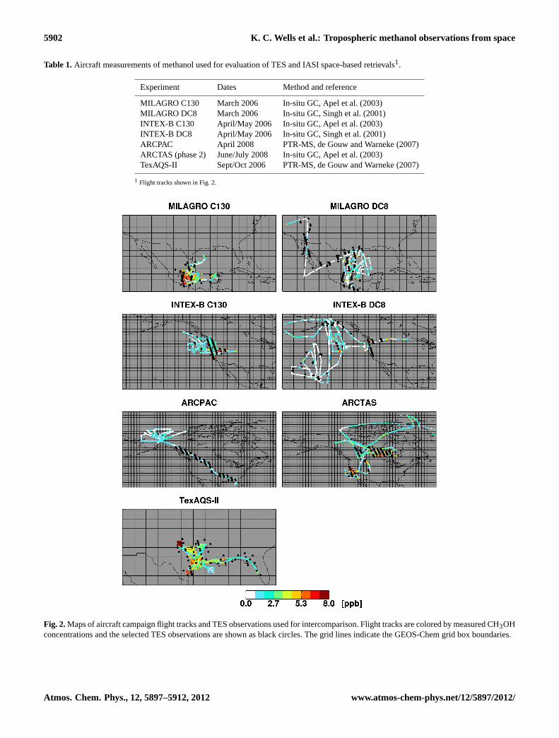
Table 1.Aircraft measurements of methanol used for evaluation of TES and IASI space-based retrievals1.

Experiment Dates Method and reference

MILAGRO C130 March 2006 In-situ GC, Apel et al. (2003)MILAGRO DC8 March 2006 In-situ GC, Singh et al. (2001)INTEX-B C130 April/May 2006 In-situ GC, Apel et al. (2003)INTEX-B DC8 April/May 2006 In-situ GC, Singh et al. (2001)ARCPAC April 2008 PTR-MS, de Gouw and Warneke (2007)ARCTAS (phase 2) June/July 2008 In-situ GC, Apel et al. (2003)TexAQS-II Sept/Oct 2006 PTR-MS, de Gouw and Warneke (2007)

1 Flight tracks shown in Fig. 2.

Fig. 2.Maps of aircraft campaign flight tracks and TES observations used for intercomparison. Flight tracks are colored by measured CH3OHconcentrations and the selected TES observations are shown as black circles. The grid lines indicate the GEOS-Chem grid box boundaries.

Atmos. Chem. Phys., 12, 5897–5912, 2012 www.atmos-chem-phys.net/12/5897/2012/

K. C. Wells et al.: Tropospheric methanol observations from space 5903

datapoints for the latter comparisons. The TES:model com-parisons then provide a measure of the TES data reliabilitybased on the extent to which they are consistent with thecorresponding aircraft:model regressions. Figure 2 illustratesthe spatial sampling of the TES measurements and flight dataemployed in these comparisons, along with the GEOS-Chemgrid resolution.

We also include IASI column retrievals in the comparison,though the IASI data are from 2009, so they do not corre-spond directly to the time period of the in situ observations.In this case, we apply the IASI land and ocean averaging ker-nels and a priori profiles to the GEOS-Chem output for 2009at the approximate time of the IASI observations in the samemanner as we do for the TES observations (Eq. (1)). We thenconvert the sampled model profile to a total column valuefor comparison with IASI. Currently, only a monthly-mean(0.5◦

×0.5◦) product from IASI is available, so we averagethe model output over the same time period. We aggregatethe IASI data to the GEOS-Chem resolution and restrict theIASI:model comparisons to the same gridboxes that were re-tained for the TES:model and aircraft:model comparisons.

Results of the satellite-model-aircraft cross-comparisonsare shown in Fig. 3 for TES retrievals with DOFS>0.5. Ini-tial analyses revealed that the TES data contain two popu-lations split by a DOFS threshold of∼0.5. Retrievals withDOFS below 0.5 tend to agree well with the simulated valuesfrom GEOS-Chem, falling around the 1:1 line in the com-parisons (Fig. S1 in the Supplement). Retrievals with DOFS>0.5, on the other hand, though still well-correlated with themodel, tend to be higher and with a different slope comparedto the model output (Figs. 3, S1 in the Supplement). This bi-modal distribution in the TES observations reflects the factthat TES methanol retrievals with DOFS less than 0.5 tend tobe significantly influenced by the a priori (and thus fall closeto the 1:1 line since the a priori is generated using GEOS-Chem). This result was also found for the TES ammonia re-trieval (Shephard et al., 2011), and suggests a general thresh-old for information content in retrievals of trace gases with aweak tropospheric signal. Cady-Pereira et al. (2012) discussthis point in greater detail. The IASI data show evidence ofa similar bimodal distribution compared to the model (e.g.,in the INTEX-B comparisons in Figs. 3 and S1 in the Sup-plement). However, the IASI methanol data do not provide adirect way to remove this effect, since the brightness temper-ature retrieval approach does not enable computation of theDOFS for each scene. The fact that TES methanol retrievalswith DOFS>0.5 are generally higher than the simulated val-ues from GEOS-Chem suggests a source underestimate forthe spatial-temporal domain of these comparisons.

For the INTEX-B comparisons in Fig. 3, the TES re-trievals are consistent with both the C-130 and DC-8 air-borne measurements. In both cases, the TES:model slopeis statistically indistinguishable from the corresponding air-craft:model slope, and the correlation coefficients are alsovery similar. In the case of MILAGRO, the C-130 data con-

tain a pronounced urban influence as sampling was focusedover Mexico City; TES exhibits lower concentrations (anda higher correlation with the model) because its orbit didnot track directly over Mexico City (Fig. 2). For the DC-8flight tracks during MILAGRO, neither the TES nor the IASIdata are correlated with the model. This campaign focused onsampling Mexico City outflow during transport over the Gulfof Mexico; it may be that the satellite measurements includesome plumes that are not captured at the 2◦

×2.5◦ resolutionof GEOS-Chem.

The ARCPAC data are the only instance with an air-craft:model slope near 1, although a 1–2 ppb offset existsbetween the observations and the model. As this was a tran-sit flight for the campaign with little vertical profiling, theinfluence of near-field emissions is lower than in the othercampaigns. For ARCPAC, most of the TES RVMR valuesfall in the same range as the aircraft observations, but a fewhigh retrieved concentrations lead to an overall low correla-tion with the model. Two of these high TES values occurredover the Colorado Front Range near Colorado Springs andPueblo, and may include urban boundary-layer pollution thatwas not sampled by the aircraft. The other two occurred overcentral/eastern Oklahoma and may be influenced by largewildfires that were burning in central Oklahoma during thecampaign. For the ARCTAS campaign, the TES:model slopeis very similar to the aircraft:model slope, and with a similardegree of correlation. The TES data are low compared to theaircraft data during TexAQS-II, probably because there werefew TES observations directly over the urban core during thiscampaign (Figs. 2 and 3).

The IASI data in Fig. 3 are not strictly analogous to the in-stantaneous values from the aircraft and TES, since they aretotal column monthly-average values, but they do provide apicture that is generally consistent with the TES:model com-parisons. For those campaigns with a significant IASI-modelcorrelation (r>0.25), the slopes are all above 1.0, supportinga source underestimate in the GEOS-Chem methanol simu-lation for the domain of these comparisons.

In summary, the satellite:model comparisons appearbroadly consistent with the information provided by the air-craft data. The satellite instruments demonstrate fidelity inresolving methanol variability in the atmosphere: correlationcoefficients between the satellite and model are for the mostpart similar to the aircraft:model values, with certain excep-tions discussed above. TES:model regression slopes are sim-ilar to the aircraft:model slopes, so there is no indicationof a persistent bias in the TES data with respect to the air-craft measurements. The IASI data exhibit consistently lowerslopes than the TES:model and aircraft:model comparisons;this may be because the IASI sensitivity to methanol peakshigher in the atmosphere than does that of TES (Beer et al.,2008; Razavi et al., 2011), but it may also be partly due to theinfluence of retrievals with low DOFS that are by necessityretained in the comparison.

www.atmos-chem-phys.net/12/5897/2012/ Atmos. Chem. Phys., 12, 5897–5912, 2012

5904 K. C. Wells et al.: Tropospheric methanol observations from space

Fig. 3. Comparison of TES, IASI and airborne methanol measurements using GEOS-Chem as an intercomparison platform. Methanolabundance as modeled by GEOS-Chem (base-case simulation) is compared to aircraft (left column, ppb), TES (middle column, ppb) and IASI(right column, 1016 molec cm−2) measurements for the field campaigns shown in Fig. 2. TES data are colored according to their DOFS, andonly DOFS>0.5 are shown. Red lines correspond to a reduced major axis fit to the data (only performed forr>0.25). Uncertainty estimatescorrespond to the standard error of the regression.

5 Seasonality of biogenic methanol emissions

Recent work by Hu et al. (2011) showed that MEGANbiogenic emissions, implemented in GEOS-Chem, lead topredicted methanol concentrations that are phase-shifted sea-sonally relative to observations in the US Upper Midwest.The result is an underestimate of the pronounced photochem-ical role for methanol early in the growing season, a time of

year when methanol emissions and concentrations are high,but isoprene emissions are still relatively low. With the ex-ception of TexAQS-II, all aircraft campaign data used in thisstudy were taken during the spring and early summer monthsover North America, so the apparent model underestimatediscussed above may be at least partly attributable to thisseasonality bias. In this section we apply the TES and IASIspace-borne observations to address this issue, and derive

Atmos. Chem. Phys., 12, 5897–5912, 2012 www.atmos-chem-phys.net/12/5897/2012/

K. C. Wells et al.: Tropospheric methanol observations from space 5905

new top-down information on the seasonality of biogenicmethanol emissions.

5.1 Methanol emissions as a function of leaf age andplant functional type

A limited number of laboratory enclosure studies and above-canopy measurements have been conducted to examinemethanol emissions from different plant species at vari-ous stages of leaf growth. It is currently understood thatplants produce methanol via dimethylation of pectin duringcell wall expansion (Galbally and Kirstine, 2002) and thusemit more methanol during their growing period. Huve etal. (2007) found that emissions were 4× higher for youngversus mature leaves of eastern cottonwood, while Nemecek-Marshall et al. (1995) found that emission rates decreased bynearly a factor of 20 between the youngest and oldest leavesof the same species. MacDonald and Fall (1993) found thatemission rates from fully expanded leaves dropped by∼2–10× from the rates of young leaves. Harley et al. (2007) re-ported that emissions from young leaves can be at least anorder of magnitude higher than those from mature leaves ofthe same plant. A recent study by Bracho-Nunez et al. (2011)showed that methanol emission rates from young leaves ofseveral Mediterranean plant species were 25–90 % higherthan those from the mature leaves. Karl et al. (2003) mea-sured springtime fluxes of methanol that were 1.7× higher inspring than in fall over a hardwood forest in northern Michi-gan, and Custer and Schade (2005) found that methanolemissions from a sugar beet field were an order of magnitudehigher in the early part of the growing season than in mid-to-late summer. Taken together, these studies provide clearevidence of enhanced methanol emissions in younger versusolder leaves, but the observed variability raises a challengein terms of implementing the phenomenon in a robust way inglobal emission models.

5.2 Application of space- based observations toconstrain seasonal emissions

To better quantify the seasonality of methanol emissions, wecompare total column amounts simulated by MEGANv2.1and GEOS-Chem to those measured by IASI over selectedtemperate regions of the globe. We use IASI for this compar-ison because of the sampling statistics provided by its highspatial and temporal resolution, which minimize any influ-ence from random error. We will then employ the TES data,with its higher spectral resolution, as an independent test ofthe results. We focus our analysis on midlatitude regions ofthe Northern Hemisphere without significant biomass burn-ing influence. Regions were defined as shown in Fig. S2 inthe Supplement: western US, eastern US, southern Canada,Europe, and southern Siberia. The fractional coverage foreach of the MEGAN PFTs in these regions is listed in Ta-ble 2, and the total emissions by source for each region are

Fig. 4. Seasonal cycle in atmospheric methanol over midlati-tudes for 2009. Shown are methanol column amounts simulatedby GEOS-Chem (base-case simulation, red solid line) and mea-sured by IASI (black solid line), and representative volume mixingratios (RVMR) simulated by GEOS-Chem (base-case simulation,red dashed line) and measured by TES (black dashed line). TESRVMR data include only those observations with DOFS>0.5. Thedata represent an average over the northern midlatitude regions ofFig. S2, and shaded areas show the standard error about the mean.

listed in Table S1 in the Supplement. The modeled biogenicsource dominates in all of these regions.

Figure 4 shows timelines of methanol abundance asmeasured by IASI (total column, molec cm−2) and TES(RVMR, ppb), and simulated by GEOS-Chem, averaged overthe midlatitude regions of Fig. S2 for 2009. As above, wesample the model to account for the vertical sensitivity ofeach satellite sensor and to minimize any influence from thea priori on the comparisons. Both the TES and IASI ensem-bles exhibit the same seasonal offset compared to the modelas was observed by Hu et al. (2011) over the US Upper Mid-west, with the observed seasonal peak occurring one monthearlier than in the simulation. The TES and IASI datasetsare seasonally in-phase, both showing the largest discrepancywith respect to the model during springtime. Figure 5 showsmethanol column timelines for 2009 as measured by IASIand simulated by GEOS-Chem for the five regions that madeup the ensemble mean in Fig. 4. The figures also includethe individual model contributions from biogenic and othersources. As we see, the biogenic source clearly drives theseasonality of the simulated methanol column in all of theseregions, serving as the major source of atmospheric methanolduring spring, summer and fall.

The comparisons in Fig. 5 show that the methanol sourceunderestimate in MEGAN+GEOS-Chem occurs predomi-nantly during springtime. It is also especially pronouncedin the western US; the GEOS-Chem column amounts wouldneed to be increased by nearly 2× over this region to matchthose observed from IASI. Our comparisons above withNorth American aircraft observations are consistent withthese findings. The results point to a misrepresentation ofthe seasonality of biogenic methanol emissions, as well as

www.atmos-chem-phys.net/12/5897/2012/ Atmos. Chem. Phys., 12, 5897–5912, 2012

5906 K. C. Wells et al.: Tropospheric methanol observations from space

Table 2.Percent coverage of plant functional types in the MEGAN landcover database for selected midlatitude regions1.

Region % Broadleaf trees % Needleleaf trees % Shrubs % Grasses % Crops

W. US 1.6 11.1 14.5 29.6 11.5E. US 20.1 18.2 8.3 11.7 29.4S. Canada 1.6 37.4 24.9 12.0 6.9Europe 8.5 20.1 9.7 12.1 37.0S. Siberia 2.4 36.8 26.8 16.0 5.2

1 Region boundaries are shown in Fig. S2.

Fig. 5. Seasonal source contributions to atmospheric methanol forthe northern midlatitude regions of Fig. S2 in the Supplement:Western US (35–50◦ N, 120–100◦ W), Eastern US (35–50◦ N, 100–60◦ W), Southern Canada (50–60◦N, 130–60◦ W), Europe (40–50◦ N, 0–30◦ E), and Southern Siberia (50–65◦ N, 80–140◦ E).Shown are 2009 timelines of the methanol column as measured byIASI (black) and simulated by GEOS-Chem (base-case simulation,red). The individual model contributions from biogenic (green) andall other sources (blue) are also shown. Lines show the mean overeach region.

a potential missing source in the western US. Other sourcesof error that could influence the simulated seasonal cycle in-clude model meteorology and methanol sinks (i.e., dry depo-sition and OH oxidation). However, these cannot explain theobserved seasonal discrepancy, which is apparent over mid-latitude landscapes around the world. Sensitivity runs em-ploying alternate OH (archived from an earlier model ver-sion) and meteorological fields (GEOS-4), and allowing forreactive uptake of methanol (Karl et al., 2010), all result in anegligible change to the seasonal cycles shown in Figs. 4 and5. We also do not find a seasonal bias in simulated methanolconcentrations over oceans, indicating that air-sea exchangedoes not contribute to the observed seasonal discrepancy overland.

Fig. 6. 2009 timelines of the percent difference in the total col-umn methanol from GEOS-Chem for a 10 % increase in the relativeemissions from new leaves (red), growing leaves (green), matureleaves (blue), and old leaves (black) for the five regions consideredin this study (Fig. S2). Lines show the mean over each region.

We thus apply the IASI data to derive optimal relativeemission rates for the different leaf age categories in termsof reproducing observed seasonal patterns in atmosphericmethanol. Four simulations were performed in which the rel-ative emission rates for new, growing, mature, and old leaveswere individually increased by 10 %. The resulting fractionalincreases in the simulated methanol column (sampled ac-cording to the IASI sensitivity) are shown in Fig. 6 for thefive midlatitude regions considered. Increases in the rela-tive emission rates of new and growing leaves manifest asincreases in atmospheric methanol during spring, while in-creases for mature and old leaves are strongest during latesummer and fall, respectively. Using these sensitivities, wederive a set of optimized relative emission factors by fittingto an area-weighted mean of the IASI observations over thefive regions of interest. The fit is derived using a constrainedmultivariate linear regression routine, in which the optimizedparameters are not permitted to decrease by more than 90 %of their original value. As our focus here is on the seasonality

Atmos. Chem. Phys., 12, 5897–5912, 2012 www.atmos-chem-phys.net/12/5897/2012/

K. C. Wells et al.: Tropospheric methanol observations from space 5907

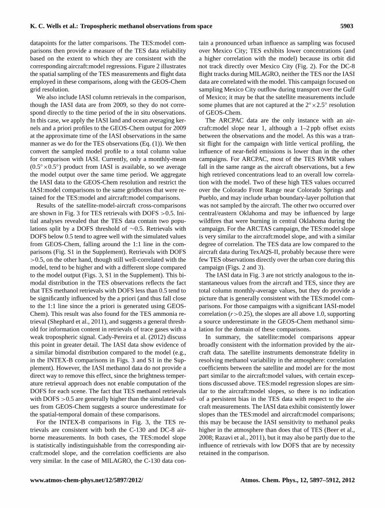
Fig. 7.Seasonal cycle in atmospheric methanol over midlatitudes asmeasured by IASI (black) and predicted by the GEOS-Chem base-case (red) and optimized (green) simulations. Data are for 2009 andare normalized by the annual mean in each case. Lines show themean over all midlatitude regions of Fig. S2, while shaded areasindicate the standard error about the mean.

of emissions rather than the absolute amount, we fit the IASIcolumn normalized by its annual mean.

Despite the fact that emissions from new and growingleaves peak during spring (Fig. 6), our initial optimization at-tempts were unable to close the satellite:model discrepancyat that time of year. IncreasingAnew has only a marginal ef-fect on springtime emissions because the increase is dampedby low values ofγ LAI . One reason for the large model biasat this time of year could thus be an underestimate in theMODIS LAI product for new and expanding canopies. It isalso possible that additional sources of methanol not cur-rently represented in MEGAN, such as leaf buds, soil emis-sions (Schade and Custer, 2004), or snowmelt (e.g. Lap-palainen et al., 2009), contribute to the early season discrep-ancy. To address this, we setγ LAI = 0.5 (corresponding to anLAI of ∼1.2) when the leaf canopy is expanding, and use thestandard PCEEA formulation (Guenther et al., 2006) whenthe canopy is static or declining. Theγ LAI value of 0.5 is ableto close the model-measurement gap in the early springtimewhile not corresponding to an excessively high LAI value.

We then find that revised parameters ofAnew = 11.0,Agrowing = 0.26, Amature= 0.12, andAold = 3.0 are able tocapture the seasonality observed in the IASI midlatitudemethanol measurements. These optimized parameters repre-sent a∼40× difference in emissions between new and grow-ing leaves, and a∼2× difference in emissions between grow-ing and mature leaves. As discussed above, methanol emis-sions have been observed to decrease by an order of mag-nitude or more between new and mature leaves, so thesesatellite-derived parameters have some consistency with insitu observations. They do represent a larger decrease thansome in situ studies suggest but, as is later shown, these newrelative emission factors provide a much more realistic sim-ulation of atmospheric methanol seasonality across midlat-itude ecosystems. Emissions from old leaves are increasedto match observed column amounts in the fall. This likely re-

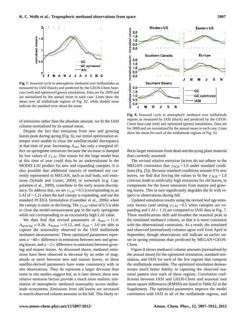
Fig. 8. Seasonal cycle in atmospheric methanol over midlatituderegions as measured by IASI (black) and predicted by the GEOS-Chem base-case (red) and optimized (green) simulations. Data arefor 2009 and are normalized by the annual mean in each case. Linesshow the mean for each of the midlatitude regions of Fig. S2.

flects larger emissions from dead and decaying plant materialthan currently assumed.

The revised relative emission factors do not adhere to theMEGAN convention thatγAGE = 1.0 under standard condi-tions (Eq. (5)). Because standard conditions assume 0 % newleaves, we find that forcing the values to fit theγ AGE = 1.0criterion leads to artificially high emissions for old leaves, tocompensate for the lower emissions from mature and grow-ing leaves. This in turn significantly degrades the fit with re-spect to observations during fall.

Updated simulation results using the revised leaf age emis-sion factors (and settingγ LAI = 0.5 when canopies are ex-panding and LAI< 1.2) are compared to IASI data in Fig. 7.These modifications shift and broaden the seasonal peak inthe simulated methanol column, so that it is more consistentwith the observational constraints. As a result, the simulatedand observed (normalized) columns agree well from April toSeptember, though observations still indicate an earlier on-set in spring emissions than predicted by MEGAN+GEOS-Chem.

Figure 8 shows methanol column amounts (normalized bythe annual mean) for the optimized simulation, standard sim-ulation, and IASI for each of the five regions that composethe midlatitude ensemble. The optimized simulation demon-strates much better fidelity in capturing the observed sea-sonal pattern over each of these regions. Correlation coef-ficients between IASI and GEOS-Chem and seasonal rootmean square differences (RMSD) are listed in Table S2 in theSupplement. The optimized parameters improve the modelcorrelation with IASI in all of the midlatitude regions, and

www.atmos-chem-phys.net/12/5897/2012/ Atmos. Chem. Phys., 12, 5897–5912, 2012

5908 K. C. Wells et al.: Tropospheric methanol observations from space

Fig. 9.Seasonal cycle in atmospheric methanol over midlatitude re-gions as measured by TES (black, for DOFS>0.5) and predictedby the GEOS-Chem base-case (red) and optimized (green) simu-lations. Data are for 2009 and are normalized by the annual meanin each case. Lines show the mean for each region (Fig. S2), whileshaded areas indicate the standard error about the mean.

reduce the model-measurement difference in the spring. Wealso examined the effect of the optimized relative emissionfactors on simulated methanol amounts in the tropics; overallemissions were slightly reduced, and in some areas the sea-sonal amplitude is now larger than observed. Our revised leafage emission parameters are therefore recommended for tem-perate but not for tropical ecosystems.

For some of the cases in Fig. 8, the simulated seasonalamplitude is weaker (e.g., Europe) or stronger (e.g., south-ern Siberia) than observed, though the phase is accurate.Model-measurement RMSD values in winter and summerare somewhat larger post-optimization in these regions. Suchdiscrepancies indicate a need for improved estimates of abso-lute methanol emission rates (rather than their seasonal tim-ing) for different plant functional types in the midlatitudes,or possibly for improved estimates of other, non-biogenic,sources of methanol.

Comparisons with independent data from TES providesupport for our revised leaf age emission factors. Figure 9shows TES global survey retrievals for 2009 over the samefive midlatitude regions used above. Only retrievals withDOFS>0.5 are included. As with IASI, the TES retrievalsreveal a late spring/early summer peak in atmosphericmethanol over midlatitude ecosystems, which is better cap-tured by the optimized simulation. The model-measurementcorrelation is improved in the optimized simulation (withthe exception of the western US), and the spring model-measurement RMS differences are reduced in all regionsexcept Europe. Over all five regions the TES observationsexhibit weaker seasonality than MEGAN+GEOS-Chem or

Fig. 10. Seasonal cycle in atmospheric methanol at North Amer-ican surface sites. Observations from Thompson Farm in NH,USA (January–December 2008), Blodgett Forest in CA, USA (May2000–April 2001), and the KCMP tall tower in MN, USA (January–December 2010), are compared to modeled concentrations from theGEOS-Chem base-case (red) and optimized (green) simulations.Concentrations are normalized to the annual mean in each case.Model results for Blodgett Forest are for 2009 rather than 2000–2001. Lines show the monthly mean values, while shaded areas in-dicate the standard error about the mean.

IASI. This may partly reflect retrieval uncertainty and re-duced sampling statistics during months when methanol con-centrations are low.

Figure 10 shows in situ measurements (normalized bythe annual mean) from Thompson Farm in New Hampshire(43.11◦ N, 70.95◦ W, 24 m a.s.l.) (Jordan et al., 2009), theBlodgett Forest Research Station in California (38.90◦ N,120.63◦ W, 1315 m a.s.l.) (Schade and Goldstein, 2006), andthe KCMP tall tower in Minnesota (44.69◦ N, 93.07◦ W,534 m a.s.l.) (Hu et al., 2011). The optimized simulationgives a better representation of the timing of the seasonalpeak in each case, and reduces the summertime RMSD at theKCMP tall tower and Blodgett Forest. Normalized methanolabundance during spring and summer appears to be too highin the optimized simulation at the KCMP tall tower and atThompson Farm; this is in part because the model underes-timates winter methanol concentrations at both sites, so theseasonal amplitude is overly pronounced. Additionally, localsources of methanol at each site may not be well captured bythe 2◦×2.5◦ simulation.

Although the optimized simulation yields a seasonal cy-cle for atmospheric methanol that is more accurate basedon midlatitude observations, key discrepancies still exist interms of the absolute concentrations. Over the western US,simulated column amounts are still a factor of two lower thanthe IASI observations (Fig. S3 in the Supplement). At Blod-gett, absolute surface concentrations in the model are 4–10×

Atmos. Chem. Phys., 12, 5897–5912, 2012 www.atmos-chem-phys.net/12/5897/2012/

K. C. Wells et al.: Tropospheric methanol observations from space 5909

lower than observed. This discrepancy could be due to thefact that this particular measurement site is located in an areaof complex terrain, but it is also consistent with a missingregional source in the model.

6 Summary and conclusions

We evaluated new retrievals of tropospheric methanol fromthe Tropospheric Emission Spectrometer (TES) and the In-frared Atmospheric Sounding Interferometer (IASI), andused them in conjunction with the GEOS-Chem CTM(driven with MEGAN emissions) to better quantify the sea-sonality of methanol emissions from terrestrial plants in tem-perate ecosystems. The TES retrievals show good agreementwith aircraft observations for retrievals with DOFS>0.5.The TES data exhibit higher concentrations compared to themodel than do the IASI data, which may reflect differing ver-tical sensitivity for the two sensors or the inclusion of re-trievals with low DOFS in the IASI data.

A full year of IASI and TES retrievals over midlatitude re-gions of the Northern Hemisphere revealed a clear seasonaloffset in the timing of model emissions, with peak concentra-tions occurring 1–2 months too late in the model. We appliedthe satellite data to derive a more robust global constraint onthe change in methanol emission rate as a function of leafage in midlatitude ecosystems. We find that the seasonalityin atmospheric methanol as measured by IASI over key mid-latitude regions is well-captured using revised relative emis-sions factors of 11.0, 0.26, 0.12, and 3.0 for new, growing,mature, and old leaves, respectively. These parameters rep-resent an increase in emissions for new and old leaves, anda decrease for growing and mature leaves compared to thestandard model. Implementing these optimized emission fac-tors in the model, and employing a leaf area index activityfactor of 0.5 for expanding canopies with LAI< 1.2, leads toa seasonal cycle in atmospheric methanol that is more con-sistent with the IASI measurements, as well as with indepen-dent data from TES. These relative emission factors for thedifferent leaf age classes were derived with respect to mid-latitude observations and are not necessarily applicable to thetropics.

While our findings here should enable more accurate sim-ulations of atmospheric methanol in temperate regions of theworld, some key issues remain to be resolved. For exam-ple, large underestimates in the overall source magnitude stillexist in areas such as the western US, pointing to a miss-ing regional source in the model. Based on observations byGeron et al. (2006), it is possible that emissions from desertshrubs are currently underestimated in MEGAN, but this re-quires further investigation. The contribution of depositionand OH oxidation to the methanol underestimate also war-rants further study. The new global datasets from TES andIASI should provide powerful new constraints for improv-

ing present understanding of methanol emissions for differ-ent plant functional types.

Supplementary material related to this article isavailable online at:http://www.atmos-chem-phys.net/12/5897/2012/acp-12-5897-2012-supplement.pdf.

Acknowledgements.This work was supported by NASA throughthe Atmospheric Chemistry Modeling and Analysis Program (Grant#NNX10AG65G), by NSF through the Atmospheric ChemistryProgram (Grant #0937004), and also by the University of Min-nesota Supercomputing Institute. The constrained linear regressionwas performed using code developed by Michele Cappellari. Wegratefully thank John Worden and Ming Luo for their role indeveloping the TES methanol retrieval. We thank Alex Guentherfor his help and suggestions in refining this work. We also thankGunnar Schade for providing the Blodgett Forest measurements.IASI has been developed and built under the responsibility of theCentre National d‘Etudes Spatiales (CNES, France). It is flownonboard the MetOp satellites as part of the EUMETSAT PolarSystem. The IASI level 1 data are distributed in near real timeby EUMETSAT through the Eumetcast dissemination system.L. Clarisse is a Postdoctoral Researcher (Charge de Recherches)and P. F. Coheur is a Research Associate (Chercheur Qualifiee)with F.R.S.-FNRS.

Edited by: L. Ganzeveld

References

Andreae, M. O. and Merlet, P.: Emission of trace gases and aerosolsfrom biomass burning, Global Biogeochem. Cy., 15, 955–966,doi:10.1029/2000GB001382, 2001.

Apel, E. C., Hills, A. J., Lueb, R., Zindel, S., Eisele, S., andRiemer, D. D.: A fast-GC/MS system to measure C-2 to C-4carbonyls and methanol aboard aircraft, J. Geophys. Res., 108,8794,doi:10.1029/2002JD003199, 2003.

Auvray, M. and Bey, I.: Long-range transport to Europe: seasonalvariations and implications for the European ozone budget, J.Geophys. Res., 110, D11303,doi:10.1029/2004JD005503, 2005.

Beer, R., Glavich, T. A., and Rider, D. M.: Tropospheric emissionspectrometer for the Earth Observing System’s Aura Satellite,Appl. Opt., 40, 2356–2367, 2001.

Beer, R., Shephard, M. W., Kulawik, S. S., Clough, S. A., Eldering,A., Bowman, K. W., Sander, S. P., Fisher, B. M., Payne, V. H.,Luo, M., Osterman, G. B., and Worden, J. R.: First satellite obser-vations of lower tropospheric ammonia and methanol, Geophys.Res. Lett., 35, L09801,doi:10.1029/2008GL033642, 2008.

Bernath, P. F., McElroy, C. T., Abrams, M. C., Boone, C. D.,Butler, M., Camy-Peyret, C., Carleer, M., Clerbaux, C., Co-heur, P. F., Decola, P., DeMaziere, M., Drummond, J. R., Du-four, D., Evans, W. F. J., Fast, H., Fussen, D., Gilbert, K., Jen-nings, D. E., Llewellyn, E. J., Lowe, R. P., Mahieu, E. Mc-Connell, J. C., McHugh, M., McLeod, S. D., Michaud, R., Mid-winter, C., Nassar, R., Nichitiu, F., Nowlan, C., Rinsland, C.

www.atmos-chem-phys.net/12/5897/2012/ Atmos. Chem. Phys., 12, 5897–5912, 2012

5910 K. C. Wells et al.: Tropospheric methanol observations from space

P., Rochon, Y. J., Rowlands, N. A., Walkty, I., Wardle, D. A.,Wehrle, V., Zander, R., Zou, J.: Atmospheric Chemistry Experi-ment (ACE): mission overview, Geophys. Res. Lett., 32, L15S01,doi:10.1029/2005GL022386, 2005.

Bracho-Nunez, A., Welter, S., Staudt, M., and Kesselmeier, J.:Plant-specific volatile organic compound emission rates fromyoung and mature leaves of Mediterranean vegetation, J. Geo-phys. Res., 116, D16304,doi:10.1029/2010JD015521, 2011.

Brock, C. A., Cozic, J. Bahreini, R., Froyd, K. D., Middlebrook,A. M., McComiskey, A., Brioude, J., Cooper, O. R., Stohl, A.,Aiken, K. C., de Gouw, J. A., Fahey, D. W., Farrare, R. A.,Gao, R. S., Gore, W., Holloway, J. S., Hubler, G., Jefferson, A.,Lack, D. A., Lance, S., Moore, R. H., Murphy, D. M., Nenes, A.,Novelli, P. C., Nowak, J. B., Ogren, J. A., Peischl, J., Pierce,R. B., Pilweskie, P., Quinn, P. K., Ryerson, T. B., Schmidt,K. S., Schwarz, J. P., Sodemann, H., Spackman, J. R., Stark,H., Thomson, D. S., Thornberry, T., Veres, P., Watts, L. A.,Warneke, C: Characteristics, sources, and transport of aerosolsmeasured in spring 2008 during the Aerosol, Radiation, andCloud Processes affecting Arctic Climate (ARCPAC) Project,Atmos. Chem. Phys., 11, 2423–2453,doi:10.5194/acp-11-2423-2011, 2011.

Cady-Pereira, K. E., Shephard, M. W., Millet, D. B., Luo, M., Wells,K. C., Xiao, Y. Payne, V. H., and Worden, J.: Methanol from TESglobal observations: retrieval algorithm and seasonal and spa-tial variability, Atmos. Chem. Phys. Discuss., 12, 11823–11859,doi:10.5194/acpd-12-11823-2012, 2012.

Carpenter, L. J., Lewis, A. C., Hopkins, J. R., Read, K. A., Longley,I. D., and Gallagher, M. W.: Uptake of methanol to the NorthAtlantic Ocean surface, Global Biogeochem. Cy., 18, GB4027,doi:10.1029/2004GB002294, 2004.

Choi, W., Faloona, I. C., Bouvier-Brown, N. C., McKay, M., Gold-stein, A. H., Mao, J., Brune, W. H., LaFranchi, B. W., Co-hen, R. C., Wolfe, G. M., Thornton, J. A., Sonnenfroh, D. M.,and Millet, D. B.: Observations of elevated formaldehyde overa forest canopy suggest missing sources from rapid oxidationof arboreal hydrocarbons, Atmos. Chem. Phys., 10, 8761–8781,doi:10.5194/acp-10-8761-2010, 2010.

Clerbaux, C., Boynard, A., Clarisse, L., George, M., Hadji-Lazaro,J., Herbin, H., Hurtmans, D., Pommier, M., Razavi, A., Turquety,S., Wespes, C., and Coheur, P. F.: Monitoring of atmosphericcomposition using the thermal infrared IASI/MetOp sounder, At-mos. Chem. Phys., 9, 6041–6054,doi:10.5194/acp-9-6041-2009,2009.

Clough, S. A., Shephard, M. W., Worden, J., Brown, P. D., Worden,H. M., Luo, M., Rodgers, C. D., Rinsland, C. P., Goldman, A.,Brown, L., Kulawik, S. S., Eldering, A., Lampel, M., Osterman,G., Beer, R., Bowman, K., Cady-Pereira, K. E., and Mlawer,E. J.: Forward model and Jacobians for Tropospheric EmissionSpectrometer retrievals, IEEE Trans. Geosci. Remote Sens., 44,1308–1323, 2006.

Coheur, P. F., Clarisse, L., Turquety, S., Hurtmans, D., andClerbaux, C.: IASI measurements of reactive trace species inbiomass burning plumes, Atmos. Chem. Phys., 9, 5655–5667,doi:10.5194/acp-9-5655-2009, 2009.

Custer, T. G. and Schade, G. W.: Seasonal OVOC fluxes from anagricultural field planted with sugar beet, Eos Trans. AGU, 86,Fall Meet. Suppl., Abstract A51B-0060, San Francisco, USA,2005.

de Gouw, J. A., Middlebrook, A. M., Warneke, C., Goldan, P.D., Kuster, W. C., Roberts, J. M., Fehsenfeld, F. C., Worsnop,D. R., Canagaratna, M. R., Pszenny, A. A. P., Keene, W. C.,Marchewka, M., Bertman, S. B., and Bates, T. S.: Budget of or-ganic carbon in a polluted atmosphere: results from the New Eng-land Air Quality Study in 2002, J. Geophys. Res., 110, D16305,doi:10.1029/2004JD005623, 2005.

de Gouw, J. and Warneke, C.: Measurements of volatile organiccompounds in the Earth’s atmosphere using proton-transfer-reaction mass spectrometry, Mass Spectrom. Rev., 26, 223–257,2007.

Dufour, G., Boone, C. D., Rinsland, C. P., and Bernath, P. F.:First space-borne measurements of methanol inside aged south-ern tropical to mid-latitude biomass burning plumes usingthe ACE-FTS instrument, Atmos. Chem. Phys., 6, 3463–3470,doi:10.5194/acp-6-3463-2006, 2006.

Dufour, G., Szopa, S., Hauglustaine, D. A., Boone, C. D., Rins-land, C. P., and Bernath, P. F.: The influence of biogenic emis-sions on upper-tropospheric methanol as revealed from space,Atmos. Chem. Phys., 7, 6119–6129,doi:10.5194/acp-7-6119-2007, 2007.

Duncan, B. N., Logan, J. A., Bey, I., Megretskaia, I. A., Yan-tosca, R. M., Novelli, P. C., Jones, N. B., Rinsland, C. P.:Global budget of CO, 1988–1997: source estimates and vali-dation with a global model, J. Geophys. Res., 112, D22301,doi:10.1029/2007JD008459, 2007.

Galbally, I. E. and Kirstine, W.: The production of methanol byflowering plants and the global cycle of methanol, J. Atmos.Chem., 43, 195–229, 2002.

Geron, C., Guenther, A., Greenberg, J., Karl, T., and Rasmussen,R.: Biogenic volatile organic compound emissions from desertvegetation of the southwestern US, Atmos. Environ., 40, 1645-1660, 2006.

Goldan, P. D., Trainer, M., Kuster, W. C., Parrish, D. D., Carpenter,J., Roberts, J. M., Yee, J. E., and Fehsenfeld, F. C.: Measurementsof hydrocarbons, oxygenated hydrocarbons, carbon monoxide,and nitrogen oxides in an urban basin in Colorado: implicationsfor emission inventories, J. Geophys. Res., 100, 22771–22783,1995.

Guenther, A., Karl, T., Harley, P., Wiedinmyer, C., Palmer, P. I.,and Geron, C.: Estimates of global terrestrial isoprene emissionsusing MEGAN (Model of Emissions of Gases and Aerosols fromNature), Atmos. Chem. Phys., 6, 3181–3210,doi:10.5194/acp-6-3181-2006, 2006.

Harley, P., Greenberg, J., Niinemets, U., and Guenther, A.: Envi-ronmental controls over methanol emission from leaves, Biogeo-sciences, 4, 1083–1099,doi:10.5194/bg-4-1083-2007, 2007.

Heikes, B. G., Chang, W. N., Pilson, M. E. Q., Swift, E.,Singh, H. B, Guenther, A., Jacob, D. J., Field, B. D., Fall,R., Riemer, D., and Brand, L.: Atmospheric methanol bud-get and ocean implication, Global Biogeochem. Cy., 16, 1133,doi:10.1029/2002GB001895, 2002.

Holzinger, R., Warneke, C., Hansel, A., Jordan, A., Lindinger, W.,Scharffe, D. H., Schade, G., and Crutzen, P. J.: Biomass burn-ing as a source of formaldehyde, acetaldehyde, methanol, ace-tone, acetonitrile, and hydrogen cyanide, Geophys. Res. Lett., 26,1161–1164, 1999.

Holzinger, R., Jordan, A., Hansel, A. and Lindinger, W.: Methanolmeasurements in the lower atmosphere near Innsbruck (047 de-

Atmos. Chem. Phys., 12, 5897–5912, 2012 www.atmos-chem-phys.net/12/5897/2012/

K. C. Wells et al.: Tropospheric methanol observations from space 5911

grees 16′ N; 011 degrees 24′ E), Austria, Atmos. Environ., 35,2525–2532, 2001.

Hu, L., Millet, D. B., Mohr, M. J., Wells, K. C., Griffis, T. J., andHelmig, D.: Sources and seasonality of atmospheric methanolbased on tall tower measurements in the US Upper Midwest,Atmos. Chem. Phys., 11, 11145–11156,doi:10.5194/acp-11-11145-2011, 2011.

Hudman, R. C., Jacob, D. J., Turquety, S., Leibensperger, E. M.,Murray, L. T., Wu, S., Gilliland, A. B., Avery, M., Bertram, T.H., Brune, W., Cohen, R. C., Dibb, J. E., Flocke, F. M., Fried,A., Holloway, J., Neuman, J. A., Orville, R., Perring, A., Ren,X., Sachse, G. W., Singh, H. B., Swanson, A., Wooldridge, P. J.:Surface and lightning sources of nitrogen oxides over the UnitedStates: magnitudes, chemical evolution, and outflow, J. Geophys.Res., 112, D12S05,doi:10.1029/2006JD007912, 2007.

Hudman, R. C., Murray, L. T., Jacob, D. J., Millet, D. B., Tur-quety, S., Wu, S., Blake, D. R., Goldstein, A. H., Holloway,J., and Sachse, G. W.: Biogenic versus anthropogenic sourcesof CO in the United States, Geophys. Res. Lett., 35, L04801,doi:10.1029/2007GL032393, 2008.

Huve, K., Christ, M., Kleist, E., Uerlings, R., Niinemets, U., Walter,A., and Wildt, J: Simultaneous growth and emission measure-ments demonstrate an interactive control of methanol release byleaf expansion and stomata, J. Exp. Bot., 58, 1783–1793, 2007.

Jacob, D. J., Field, B. D., Li, Q. B., Blake, D. R., de Gouw,J., Warneke, C., Hansel, A., Wisthaler, A., Singh, H. B.,Guenther, A.: Global budget of methanol: constraints fromatmospheric observations, J. Geophys. Res., 110, D08303,doi:10.1029/2004JD005172, 2005.

Jacob, D. J., Crawford, J. H., Maring, H., Clarke, A. D., Dibb, J.E., Emmons, L. K., Ferrare, R. A., Hostetler, C. A., Russell, P.B., Singh, H. B., Thompson, A. M., Shaw, G. E., McCauley, E.,Pederson, J. R., Fisher, J. A.: The Arctic Research of the Compo-sition of the Troposphere from Aircraft and Satellites (ARCTAS)mission: design, execution, and first results, Atmos. Chem. Phys.,10, 5191–5212,doi:10.5194/acp-10-5191-2010, 2010.

Jordan, C., Fitz, E., Hagan, T., Sive, B., Frinak, E., Haase, K., Cot-trell, L., Buckley, S., Talbot, R.: Long-term study of VOCs mea-sured with PTR-MS at a rural site in New Hampshire with urbaninfluences, Atmos. Chem. Phys., 9, 4677–4697,doi:10.5194/acp-9-4677-2009, 2009.

Karl, T., Guenther, A., Spirig, C., Hansel, A., and Fall, R.: Sea-sonal variation of biogenic VOC emissions above a mixed hard-wood forest in northern Michigan, Geophys. Res. Lett., 30, 2186,doi:10.1029/2003GL018432, 2003.

Karl, T., Harren, F., Warneke, C., de Gouw, J., Grayless, C., andFall, R.: Senescing grass crops as regional sources of reactivevolatile organic compounds, J. Geophys. Res., 110, D15302,doi:10.1029/2005JD005777, 2005.

Karl, T., Harley, P., Emmons, L., Thornton, B., Guenther, A., Basu,C., Turnipseed, A., and Jardine, K.: Efficient atmospheric cleans-ing of oxidized organic trace gases by vegetation, Science, 330,816–819,doi:10.1126/science.1192534, 2010.

Kleb, M. M., Chen, G., Crawford, J. H., Flocke, F. M., and Brown,C. C.: An overview of measurement comparisons from theINTEX-B/MILAGRO airborne field campaign, Atmos. Meas.Tech., 4, 9–27,doi:10.5194/amt-4-9-2011, 2011.

Kuhns, H., Green, M., and Etyemezian, V.: Big Bend RegionalAerosol and Visibility Observational (BRAVO) Study Emis-

sions Inventory, Report prepared for BRAVO steering commit-tee, Desert Research Institute, Las Vegas, Nevada, USA, 2003.

Lappalainen, H. K., Sevanto, S., Back, J., Ruuskanen, T. M., Ko-lari, P., Taipale, R., Rinne, J., Kulmala, M., and Hari, P.: Day-time concentrations of biogenic volatile organic compoundsin a boreal forest canopy and their relation to environmen-tal and biological factors, Atmos. Chem. Phys., 9, 5447–5459,doi:10.5194/acp-9-5447-2009, 2009.

Macdonald, R. C. and Fall, R.: Detection of substantial emissionsof methanol from plants to the atmosphere, Atmos. Environ., 27,1709–1713, 1993.

Millet, D. B., Donahue, N. M., Pandis, S. N., Polidori, A.,Stanier, C. O., Turpin, B. J., and Goldstein, A. H.: Atmosphericvolatile organic compound measurements during the PittsburghAir Quality Study: results, interpretation, and quantification ofprimary and secondary contributions, J. Geophys. Res., 110,D07S07,doi:10.1029/2004JD004601, 2005.

Millet, D. B., Jacob, D. J., Turquety, S., Hudman, R. C., Wu, S.,Fried, A., Walega, J., Heikes, B. G., Blake, D. R., Singh, H.B., Anderson, B. E., and Clarke, A. D.: Formaldehyde distribu-tion over North America: implications for satellite retrievals offormaldehyde columns and isoprene emission, J. Geophys. Res.,111, D24S02,doi:10.1029/2005JD006853, 2006.

Millet, D. B., Jacob, D. J., Custer, T. G., de Gouw, J. A., Goldstein,A. H., Karl, T., Singh, H. B., Sive, B. C., Talbot, R. W., Warneke,C., and Williams, J.: New constraints on terrestrial and oceanicsources of atmospheric methanol, Atmos. Chem. Phys., 8, 6887–6905,doi:10.5194/acp-8-6887-2008, 2008.

Nemecek-Marshall, M., Macdonald, R. C., Franzen, F. J., Woj-ciechowski, C. L., and Fall, R.: Methanol emission from leaves:enzymatic detection of gas-phase methanol and relation ofmethanol fluxes to stomatal conductance and leaf development,Plant Physiol., 108, 1359–1368, 1995.

Olson, D. M., Dinerstein, E., Wikramanayake, E. D., Burgess, N.D., Powell, G. V. N., Underwood, E. C., D’Amico, J. A., Itoua, I.,Strand, H. E., Morrison, J. C., Loucks, C. J., Allnutt, T. F., Rick-etts, T. H., Kura, Y., Lamoreux, J. F., Wettengel, W. W., Hedao,P., and Kassem, K. R.: Terrestrial ecoregions of the world: A newmap of life on Earth, Bioscience, 51, 933–938, 2001.

Parrish, D. D., Allen, D. T., Bates, T. S., Estes, M., Fehsenfeld, F.C., Feingold, G., Ferrare, R., Hardesty, R. M., Meagher, J. F.,Nielsen-Gammon, J. W., Pierce, R. B., Ryerson, T. B., Seinfeld,J. H., Williams, E. J.: Overview of the Second Texas Air QualityStudy (TexAQS II) and the Gulf of Mexico Atmospheric Com-position and Climate Study (GoMACCS), J. Geophys. Res., 114,D00F13,doi:10.1029/2009JD011842, 2009.

Payne, V. H., Clough, S. A., Shephard, M. W., Nassar, R., and Lo-gan, J. A.: Information-centered representation of retrievals withlimited degrees of freedom for signal: application to methanefrom the Tropospheric Emission Spectrometer, J. Geophys. Res.,114, D10307,doi:10.1029/2008JD010155, 2009.

Razavi, A., Karagulian, F., Clarisse, L., Hurtmans, D., Coheur, P.F., Clerbaux, C., Muller, J. F., and Stavrakou, T.: Global distribu-tions of methanol and formic acid retrieved for the first time fromthe IASI/MetOp thermal infrared sounder, Atmos. Chem. Phys.,11, 857–872,doi:10.5194/acp-11-857-2011, 2011.

Rodgers, C. D.: Inverse Methods for Atmospheric Sounding: The-ory and Practice, World Scientific, Tokyo, Japan, 2000.

www.atmos-chem-phys.net/12/5897/2012/ Atmos. Chem. Phys., 12, 5897–5912, 2012

5912 K. C. Wells et al.: Tropospheric methanol observations from space

Schade, G. W. and Custer, T. G.: OVOC emissions fromagricultural soil in northern Germany during the 2003European heat wave, Atmos. Environ., 38, 6105–6114,doi:10.1016/j.atmosenv.2004.08.017, 2004.

Schade, G. W. and Goldstein, A. H.: Seasonal measurementsof acetone and methanol: abundances and implications foratmospheric budgets, Global Biogeochem. Cy., 20, GB1011,doi:10.1029/2005GB002566, 2006.

Shephard, M. W., Cady-Pereira, K. E., Luo, M., Henze, D. K., Pin-der, R. W., Walker, J. T., Rinsland, C. P., Bash, J. O., Zhu, L.,Payne, V. H., and Clarisse, L.: TES ammonia retrieval strat-egy and global observations of the spatial and seasonal vari-ability of ammonia, Atmos. Chem. Phys., 11, 10743–10763,doi:10.5194/acp-11-10743-2011, 2011.

Singh, H. B, Chen, Y., Staudt, A., Jacob, D., Blake, D., Heikes, B.,and Snow, J.: Evidence from the Pacific troposphere for largeglobal sources of oxygenated organic compounds, Nature, 410,1078–1081, 2001.

Singh, H. B., Salas, L. J., Chatfield, R. B., Czech, E., Fried,A., Walega, J., Evans, M. J., Field, B. D., Jacob, D. J.,Blake, D., Heikes, B., Talbot, R., Sachse, G., Crawford, J.H., Avery, M. A., Sandholm, S., and Fuelberg, H.: Analy-sis of the atmospheric distribution, sources, and sinks of oxy-genated volatile organic chemicals based on measurements overthe Pacific during TRACE-P, J. Geophys. Res., 109, D15S07,doi:10.1029/2003JD003883, 2004.

Singh, H. B., Brune, W. H., Crawford, J. H., Flocke, F., and Ja-cob, D. J.: Chemistry and transport of pollution over the Gulfof Mexico and the Pacific: spring 2006 INTEX-B campaignoverview and first results, Atmos. Chem. Phys., 9, 2301–2318,doi:10.5194/acp-9-2301-2009, 2009.

Stavrakou, T., Mueller, J. F., De Smedt, I., Van Roozendael,M., van der Werf, G. R., Giglio, L., and Guenther, A.:Global emissions of non-methane hydrocarbons deduced fromSCIAMACHY formaldehyde columns through 2003–2006, At-mos. Chem. Phys., 9, 3663–3679,doi:10.5194/acp-9-3663-2009,2009.

Stavrakou, T., Guenther, A., Razavi, A., Clarisse, L., Clerbaux,C., Coheur, P. F., Hurtmans, D., Karagulian, F., De Maziere,M., Vigouroux, C., Amelynck, C., Schoon, N., Laffineur,Q., Heinesch, B., Aubinet, M., Rinsland, C., and Muller,J. F.: First space-based derivation of the global atmosphericmethanol emission fluxes, Atmos. Chem. Phys., 11, 4873–4898,doi:10.5194/acp-11-4873-2011, 2011.

Tie, X., Guenther, A., and Holland, E.: Biogenic methanol and itsimpacts on tropospheric oxidants, Geophys. Res. Lett., 30, 1881,doi:10.1029/2003GL017167, 2003.

Tyndall, G. S., Cox, R. A., Granier, C., Lesclaux, R., Moortgat, G.K., Pilling, M. J., Ravishankara, A. R., and Wallington, T. J.:Atmospheric chemistry of small organic peroxy radicals, J. Geo-phys. Res., 106, 12157–12182, 2001.

van der Werf, G., Randerson, J., Giglio, L., Collatz, G., Kasibhatla,P., and Arellano, A.: Interannual variability in global biomassburning emissions from 1997 to 2004, Atmos. Chem. Phys., 6,3423–3441,doi:10.5194/acp-6-3423-2006, 2006.

Vestreng, V. and Klein, H.: Emission data reported to UN-ECE/EMEP: Quality assurance & presentation of WebDab, Nor-weigian Meterological Institute, Oslo, Norway, MSC-W StatusReport, 2002.

Warneke, C., Karl, T., Judmaier, H., Hansel, A., Jordan, A.,Lindinger, W., and Crutzen, P. J.: Acetone, methanol, andother partially oxidized volatile organic emissions from deadplant matter by abiological processes: significance for atmo-spheric HOx chemistry, Global Biogeochem. Cy., 13, 9–17,doi:10.1029/98GB02428, 1999.

Warneke, C., McKeen, S. A., de Gouw, J. A., Goldan, P. D.,Kuster, W. C., Holloway, J. S., Williams, E. J., Lerner, B. M.,Parrish, D. D., Trainer, M., Fehsenfeld, F. C., Kato, S., At-las, E. L., Baker, A., and Blake, D. R.: Determination of ur-ban volatile organic compound emission ratios and comparisonwith an emissions database, J. Geophys. Res., 112, D10S47,doi:10.1029/2006JD007930, 2007.

Williams, J., Holzinger, R., Gros, V., Xu, X., Atlas, E., and Wallace,D. W. R.: Measurements of organic species in air and seawa-ter from the tropical Atlantic, Geophys. Res. Lett., 31, L23S06,doi:10.1029/2004GL020012, 2004.

Xiao, Y., Cady-Pereira, K. E., Payne, V. H., Millet, D. B., Shep-hard, M. W., Luo, M., Alvarado, M., Wells, K. C., Apel, E. C.,Campos, T. L., Singh, H. B., and Sachse, G. W.: Methanol-COcorrelations in Mexico City pollution outflow from aircraft andsatellite during MILAGRO, Atmos. Chem. Phys. Discuss., 12,5705–5738,doi:10.5194/acpd-12-5705-2012, 2012.

Yang, W., Shabanov, N. V., Huang, D., Wang, W., Dickinson, R. E.,Nemani, R. R., Knyazikhin, Y., and Myneni, R. B.: Analysis ofleaf area index products from combination of MODIS Terra andAqua data, Remote Sens. of Environ., 104, 297–312, 2006.

Zhang, Q., Streets, D. G., Carmichael, G. R., He, K. B., Huo, H.,Kannari, A., Klimont, Z., Park, I. S., Reddy, S., Fu, J. S., Chen,D., Duan, L., Lei, Y., Wang, L. T., and Yao, Z. L.: Asian emis-sions in 2006 for the NASA INTEX-B mission, Atmos. Chem.Phys., 9, 5131–5153,doi:10.5194/acp-9-5131-2009, 2009.

Atmos. Chem. Phys., 12, 5897–5912, 2012 www.atmos-chem-phys.net/12/5897/2012/