HAL Id: hal-00667122https://hal.archives-ouvertes.fr/hal-00667122

Submitted on 7 Feb 2012

HAL is a multi-disciplinary open accessarchive for the deposit and dissemination of sci-entific research documents, whether they are pub-lished or not. The documents may come fromteaching and research institutions in France orabroad, or from public or private research centers.

L’archive ouverte pluridisciplinaire HAL, estdestinée au dépôt et à la diffusion de documentsscientifiques de niveau recherche, publiés ou non,émanant des établissements d’enseignement et derecherche français ou étrangers, des laboratoirespublics ou privés.

Tropical deforestation modelling : a comparative analysisof different predictive approaches. The case study of

Peten, Guatemala.Marco Follador, Nathalie Villa, Martin Paegelow, Fernanda Renno, Roberto

Bruno

To cite this version:Marco Follador, Nathalie Villa, Martin Paegelow, Fernanda Renno, Roberto Bruno. Tropical de-forestation modelling : a comparative analysis of different predictive approaches. The case study ofPeten, Guatemala.. Modelling Environmental Dynamics, Springer, pp.77-108, 2008, <10.1007/978-3-540-68498-5_3>. <hal-00667122>

TROPICAL DEFORESTATION MODELLING: A COMPARATIVE ANALYSIS OF DIFFERENT PREDICTIVE APPROACHES.

THE CASE STUDY OF PETEN, GUATEMALA M. Follador a,b, N. Villac, M. Paegelowa, F.Rennoa, R.Brunob.

a GEODE/CNRS, University of Toulouse II , 5 allées A. Machado, 31058 Toulouse, France b DICMA, University of Bologna, Viale Risorgimento 2, 40100 Bologna, Italy

c CICT, University of Toulouse III, 118 route de Narbonne, 31062 Toulouse, France marco.follador@mail.ing.unibo.it; nvilla@cict.fr; paegelow@univ-tlse2.fr ;

renno@univ-tlse2.fr; roberto.bruno@mail.ing.unibo.it

Abstract

The frequent use of predictive models for analysing of complex, natural or artificial, phenomena is changing the traditional approaches to environmental and hazard problems. The continuous improvement of computer performances allows more detailed numerical methods, based on space-time discretisation, to be developed and run for a predictive modeling of complex real systems, reproducing the way their spatial patterns evolve and pointing out the degree of simulation accuracy. In this contribution we present an application of several models (Geomatics, Neural Networks, Land Cover Modeler and Dinamica EGO) in a tropical training area of Peten, Guatemala. During the last decades this region, included into the Biosphere Maya reserve, has known a fast demographic raise and a subsequent uncontrolled pressure on its own geo-resources; the test area can be divided into several sub-regions characterized by different land use dynamics. Understand and quantify these differences permits a better approximation of real system; moreover we have to consider all the physic, socio-economic parameters which will be of use for represent the complex and sometime at random, human impact. Because of the absence of detailed data for our test area, nearly all information were derived from the image processing of 41 ETM+, TM and SPOT scenes; we pointed out the past environmental dynamics and we built the Input layers for the predictive models. The data from 1998 and 2000 were used during the calibration to simulate the Land Cover changes in 2003, selected as reference date for the validation. The basic statistics permit to highlight the qualities or the weaknesses for each model on the different sub-regions.

Keywords: Predictive Models; Space-time discretisation; Remote Sensing; Neural Networks; Markov Chains; MCE; Dinamica; Risk management; Deforestation; Peten; Guatemala

Resumen

La utilización cada día más frecuente de los modelos predictivos para describir sistemas complejos, naturales o artificiales, está cambiando progresivamente los enfoques tradicionales de las problemáticas medioambientales y de la gestión del riesgo. El notable potencial de las calculadoras electrónicas actuales hace posible el desarrollo de modelos numéricos de cálculo basado en una discretización espacio-temporal que permiten simular el comportamiento de fenómenos complejos así como prever situaciones futuras, con diferentes grados de aproximación. Se presenta aquí una aplicación de distintos modelos predictivos (Géomatique, Redes de Neuronas, LCM Idrisi Andes y Dinámica), en una región de bosque tropical de Peten, Guatemala. Esta región, inscrita en la reserva de biosfera Maya, a conocido en las últimas décadas, un crecimiento demográfico y una presión fuera de control sobre los recursos naturales; en la región de estudio podemos indicar sub-regiones con diferentes dinámicas de utilización del suelo.Comprender y cuantificar tales diferencias permite la obtención de una buena aproximación de la situación real, y es necesario integrar los parámetros físicos, sociales y económicos esenciales para describir el complejo, y a veces aleatorio, componente antropico. La primera fase de estudio de esta región se ha basado exclusivamente en el análisis de información de satélites, ya que no existen otros datos útiles disponibles sobre esta zona. El tratamiento de 41 imágenes ETM +, TM e SPOT ha hecho posible la observación de dinámicas medioambientales pasadas, así como la construcción de "Input" para los distintos enfoques predictivos. Los resultados obtenidos a partir de la información recogida en 1998 y 2000 serán corroborados con una imagen real de 2003; las estadísticas de base permitirán destacar los puntos fuertes y los puntos débiles de cada modelo sobre las diferentes sub-regiones.

Palabras clave: Modelos Predictivos; Discretizacìon espacio-temporal; Teledeteccìon; Redes

Neurales; Cadenas de Markov; MCE; Dinamica; Gestión del riesgo; Deforestacìon; Peten; Guatemala

2 TÍTULO DEL LIBRO

Résumé

L’ utilisation chaque jour plus fréquent des modèles prédictives pour décrire systèmes complexes, naturels ou artificiels, est en train de changer progressivement les approches traditionnelles des problématiques environnementales et de gestion du risque. Le remarquable potentiel des calculatrices électroniques actuelles rend possible le développement de modèles numériques de calcule basé sur une discrétisation spatio-temporelle que permettent de simuler le comportement de phénomènes complexes ainsi que prévoir des scénarios futures, avec différents dégréés d’approximation. On présent ici une application de différents modèles prédictives (Géomatique, Réseaux de Neurones, LCM Idrisi Andes et Dinamica), dans une région de forêt tropicale au Peten, Guatemala. Cette région, inscrite dans la réserve de biosphère Maya, a connu dans les dernières décades, une croissance démographique et une pression hors contrôle sur les ressources naturelles; dans la région d’étude nous pouvons signaler des sous-régions avec différentes dynamiques d’utilisation du sol. Comprendre et quantifier tels différences permet l’obtention d’une bonne approximation de la situation réel, et il est nécessaire intégrer les paramètres physiques, sociales et économiques essentielles pour décrire la complexe, et parfois aléatoire, composante anthropique. La première phase d’étude de cette région a été basée exclusivement sur l’analyse d’informations des satellites, car il n’existe pas d’autres données utiles disponibles sur cette étendue. Le traitement de 41 images ETM+, TM e SPOT a rendu possible l’observation des dynamiques environnementales passées ainsi que la construction de l’Input pour les différentes approches prédictives. Les résultats obtenues en partent des informations collectées en 1998 et 2000 seront validés avec une image réelle de 2003 ; les statistiques de base vont permettre de souligner les points fort et les points faibles de chaque modèle sur les différentes sous-régions.

Mots clefs: Modèles prédictives ; Discretisation spatio-temporelle ; télédétection ; Réseaux de Neurones ; Markov chaine ; MCE ; Dinamica ; Gestion du risque ; Déforestation ; Peten ; Guatemala

1. Introduction

1.1. Overview

The human activities in tropical forest areas determine an increasing resources consumption, often driven by demographic raise or by large-scale industrial, mining or agricultural projects. The frequent use of simulation methodologies to understand these environmental impacts and their long terms consequences represents an important tools for a rational management of hazard problems. The continuous improvement of computer performances allows more detailed numerical methods, based on space-time discretisation, to be developed and run for a predictive modeling of complex real systems, reproducing the way their spatial patterns evolve.

We remember that a model is an abstraction which simplifies the studied phenomena only considering its principal components and properties (Coquillard & Hill, 1997 ); the modeler should take several decisions which demand a deep knowledge of the model and the links between model and reality (La Moingne,1994), in order to define the objectives coherently with the available data. To better understand the complex land cover properties and the socio-economic factors which influence the human activities, it is necessary an interdisciplinary cooperation among different research areas and an integrated use of several tools and methodologies. After an exploratory analysis (what, where, when), the next step is study the causes and rules that characterize a phenomena and its evolution (how, why); the level of understanding is valued comparing the first raw model outcome with a set of experimental data, pointing out the limits of our approach and often determining some parameters previously ignored (Kavouras, 2001).

To improve the data sets, particularly where field measures are not allowed (large regions with hard environmental conditions; developing countries with political instability; research projects without time and money consumption possibilities), we can take advantage from remote sensed information; the GIS represent a powerful tool for integrated these multiscale data from ground-based and satellite images. The spatial scale of investigation may vary with the type of land cover as different parameters vary in different ways across the space (Moore et al., 1993); the choice of right support size depends on our objectives and on spatial frequencies

3

of environmental system. Moreover we have to consider the computer processing power, because a large size matrix (larger number of rows and columns due to downscaling) may demand a very long computing time and often this represents a serious obstacle for model running. In this contribution we used a pixel size of 20m by 20m that allows to satisfy both processing capabilities and accuracy of spatial pattern representation (Hengl,T., 2006), providing a finer definition of land cover and partially solving the mixed-pixel problems (Atkinson,2003; Foody, 2000).

Other important question during the model developing and calibration is the choice of temporal scale as every land cover change presents a particular spatio-temporal structure. This temporal lag must be representative of the main dynamics during the studied period but it strictly depends on data availability and on specific planning problems. If we want to project the ecological and socio-economic consequences into the immediate future we adopted an higher temporal resolution than strategic planning addressing longer terms goals (Kavouras, 2001). In this contribution we adopted a lag of approximately two years, using the data sets from 1998 and 2000 to reproduce the landscape evolution in 2003, selected as reference date for the validation.

1.2. Description of Predictive Models

Four predictive models are presented here; they simulate the land cover changes in La Joyanca region occurred from 2000 to 2003, using different theoretical approaches. The basic statistics of predicted results and the analysis of residuals point out the limits and the potentialities of each model in the different sub-regions of test areas, characterized by different environmental dynamics.

1.2.1. PNNET: Predictive Neural Networks

Here we adopted a Multi-layer Perceptron (MLP), a feed forward Neural Networks (NN) composed of three layers: the Input layer (the number of neurons depends on the number of input data, e.g., thematic maps and environmental criteria), the Output layer (the number of neurons depends on our goal, i.e. predicted land cover maps) and an intermediate Hidden layer (its size was decided performing a cross validation of NN to optimized the models). Several NN with different topology but the same Input layer, were trained using a supervised learning algorithm (error-back propagation); the best NN was selected on the basis of statistical criteria, (i.e., root mean-squared error) to minimize the difference between the real and the predicted Output (Joshi et al., 2006; Lee et al., 2006; Villa et al., 2007). The nnet function (Venables and Ripley,1999) was loaded in R© computing environment, for the training process; the R© language was used to compile our three program for producing a predictive map of land cover, freely downloaded from http://nathalie.vialaneix.free.fr/maths/article.php3?id_article=49:.

1.2.2. Geomatics model

This model derives from the integration of Markov chains analysis (MCA) for time prediction and Multi Criteria Evaluation (MCE), Multi Objective (MOLA) and cellular automata to perform a spatial allocation of simulated land cover scores. MCA of second order is a discrete process and its values at instance t+1 depend on values at instances t0 and t-1. The prediction is given as estimation of transition probabilities. MCA produces a transition matrix recording the probability that each land cover class change to each other class and the number of pixels expected to change. MCE is a method that is used to create a land cover specific suitability maps, based on the rules that link the environmental variables to the studied phenomena (deforestation).These rules can be set integrating statistical techniques with a supervised analysis of modeler. The suitability maps are used for spatial allocation of predicted time transitions. A MOLA and cellular automata are performed to integrated the predicted land cover maps and improve the spatial contiguity.

4 TÍTULO DEL LIBRO

1.2.3. Land Change Modeller: the new Idrisi Andes model

This model aggregates a Markov Chains analysis (MCA) for time prediction, Multi-layer Perceptron (MLP) and a zoning based on incentives-constraints, for a spatial allocation of simulated land cover scores. We have to use only continuous quantitative variables (PNNET can use both quantitative and qualitative variables, coded in disjunctive form). After the sample size definition, we set the number of neuron in the hidden layer and stop the model running when the accuracy rate is approximately 90%; MPL permits to repeat the training more time to achieve the desiderate error score. The classification produces two transition potential maps, which express for each pixel its potential for both deforestation and reforestation. The Change Prediction step integrates the amount of changes, calculated in MCA, with the potential maps for the modelled transitions, to produce both hard and soft classification. The last one points out all the zones with different probability to change, showing the more vulnerable spots. During this phase we can introduce an incentive-disincentive for each transition, to influence its potential map on the basis of our environmental system knowledge (e.g., future government planning, forest reserves).

1.2.4. Dinamica EGO: Environment for Geoprocessing Objects

Dinamica EGO is the new simulation model of environmental dynamics developed by the Remote Sensing Laboratory (CSR) at Federal University of Minas Gerais (UFMG), Brazil. This powerful freeware (http://www.csr.ufmg.br/dinamica/EGO ) aggregates the traditional GIS tools with several operators for simulating spatial phenomena. The model, from calibration to validation, follows a data flow in form of diagram; a friendly graphical interface permits to create models by connecting algorithms (functors) via their ports. We remark that it is possible divide the test area into sub-regions, characterized by different environmental dynamics, and apply a specific approach for each one of them (Rodrigues et al.,2006) The calibration calculates the matrix of transition rates (net rates) for a time period (initial-final landscape); a probability map of occurrence for each transition is produced, using the Weight of Evidence method. The absolute number of pixels to be changed was divided between two transition functions, Expander which analyses the expansion or contraction of precedent patches for a given category, and Patcher which generates new patches (e.g., new cleared areas). The validation produce a fuzzy similarity map (a comparison within a determined zone of influence for each cell) between real and predicted outcomes; this method considers not only the pixel by pixel agreement (hard comparison), but also the probability to find the correct value in the pixel neighbourhood.

2. Test areas and data sets

2.1. La Joyanca training site, Peten, Guatemala

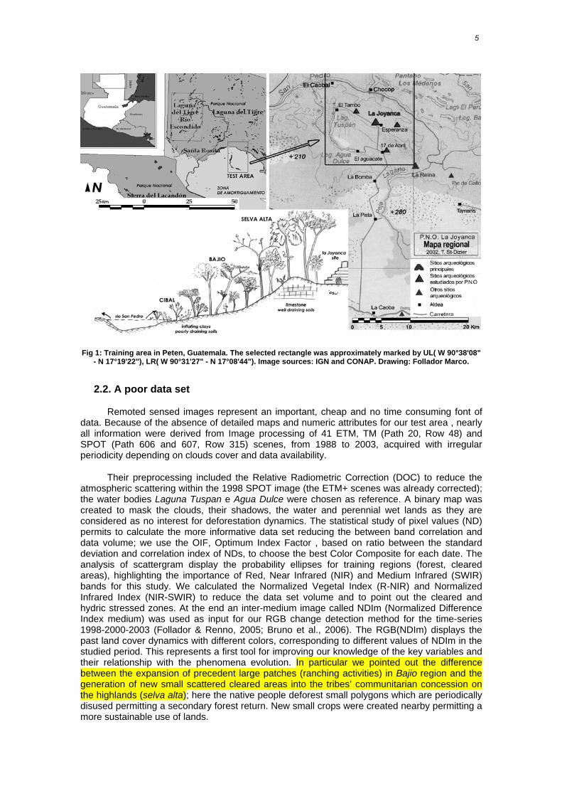
Our test area is located on the boarder between Guatemala and Mexico; it is included into the Biosphere Maya, the largest continuous tropical forest of Central America (Fig.1). Our studies were focused around La Joyanca site, Peten; it is a part of “Bosque Humedo Subtropical” (Cruz 1976) with mean annual temperature of 25°C, precipitation average fluctuating between 1160 and 1700 mm/year and a semi-evergreen tropical forest cover. The topography is generally suave with an elevation from 50 to 250 m on mean sea level (IGM, Instituto Geogràfico Militar Guatemala, Mapa 1-DMA, E754, 2067I).This region is characterized by hilly landscape with small escarps; the soils are comprised of evaporitic limestone and micro granular dolomite (Arnauld 2000). The first historical occupation of Peten with its nearly overall deforestation began during the Classic period of Maya empire and ended with its collapse and subsequent reforestation (Geoghegan et al., 2001). During the last decades this region has known a new progressive demographic raise, due to the immigration of Ladinos and native people from the south of Guatemala running away from poverty and looking for new lands. The human impact became evident after 1988 with the first settlements on the North boarder of Rio San Pedro; in the following years a fast deforestation, obtained by the traditional slash and burn technique, for agriculture and mainly for ranching activities, determined a dangerous situation for environmental sustainability (Follador & Renno. 2005).

5

Fig 1: Training area in Peten, Guatemala. The selected rectangle was approximately marked by UL( W 90°38'08" - N 17°19'22"), LR( W 90°31'27" - N 17°08'44"). Image sources: IGN and CONAP. Drawing: Follador Marco.

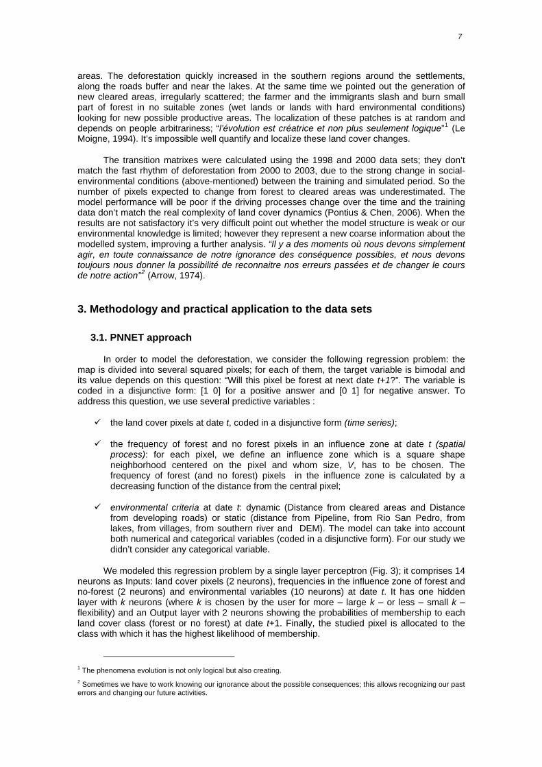
2.2. A poor data set

Remoted sensed images represent an important, cheap and no time consuming font of data. Because of the absence of detailed maps and numeric attributes for our test area , nearly all information were derived from Image processing of 41 ETM, TM (Path 20, Row 48) and SPOT (Path 606 and 607, Row 315) scenes, from 1988 to 2003, acquired with irregular periodicity depending on clouds cover and data availability.

Their preprocessing included the Relative Radiometric Correction (DOC) to reduce the atmospheric scattering within the 1998 SPOT image (the ETM+ scenes was already corrected); the water bodies Laguna Tuspan e Agua Dulce were chosen as reference. A binary map was created to mask the clouds, their shadows, the water and perennial wet lands as they are considered as no interest for deforestation dynamics. The statistical study of pixel values (ND) permits to calculate the more informative data set reducing the between band correlation and data volume; we use the OIF, Optimum Index Factor , based on ratio between the standard deviation and correlation index of NDs, to choose the best Color Composite for each date. The analysis of scattergram display the probability ellipses for training regions (forest, cleared areas), highlighting the importance of Red, Near Infrared (NIR) and Medium Infrared (SWIR) bands for this study. We calculated the Normalized Vegetal Index (R-NIR) and Normalized Infrared Index (NIR-SWIR) to reduce the data set volume and to point out the cleared and hydric stressed zones. At the end an inter-medium image called NDIm (Normalized Difference Index medium) was used as input for our RGB change detection method for the time-series 1998-2000-2003 (Follador & Renno, 2005; Bruno et al., 2006). The RGB(NDIm) displays the past land cover dynamics with different colors, corresponding to different values of NDIm in the studied period. This represents a first tool for improving our knowledge of the key variables and their relationship with the phenomena evolution. In particular we pointed out the difference between the expansion of precedent large patches (ranching activities) in Bajio region and the generation of new small scattered cleared areas into the tribes’ communitarian concession on the highlands (selva alta); here the native people deforest small polygons which are periodically disused permitting a secondary forest return. New small crops were created nearby permitting a more sustainable use of lands.

6 TÍTULO DEL LIBRO

A supervised classification was applied to more informative RGB for each date; we aggregate the MaxLikelihood Algorithm, considering the pixel by pixel probability of membership to each category and ICM (Interacted conditional Models, developed in Spring freeware: http://www.dpi.inpe.br/spring) a vicinity-method which analyses the spatial distribution of nearest pixels. The result displays 4 classes: high forest (Foresta Alta), low wet forest (Bajio), perennial wet land (Cibal) and disturbed areas (cleared areas, nude soil, crops, roads, etc.), after reduced to binary Forest-Milpa during the simulation. The word Milpa traditionally identifies a mixed crops of maize, beans and pumpkin (Effantin-Touyer, 2006), generally obtained in forest zone by the slash and burn technique; here we use “Milpa” to represent the whole loss of original closed tropical vegetation. The accuracy was very good (Kappa >0.9) for the last two categories but we have met a big confusion (25%) in separating Foresta Alta e Bajio, due to a partial spectra overlap. To improve this result a texture analyses using geostatistical tools (variogram) will be necessary.

Integrating the Image processing and GIS spatial operators we have built the environmental criteria strongly linked with landscape trajectory: several distance maps was calculated and a DEM was derived from Radar Image. No qualitative information are used.

2.3. Phenomena evolution and driving processes

There is a visible change in driving processes between the training period 1988-2000 and the simulated period 2000-2003 (Fig.2); from 1988 to 1998 the deforestation dynamics was clearly concentred on the north side of Rio San Pedro which represented for a long time the main way of access to the region. These lands are more elevated than the southern ones which are periodically flooded during the rainy season. The cleared areas presented a regular geometric form and they are mainly used for maize crops and pasture. The clearing progression was driven by the expansion of previous patches and, secondarily, by the generation of new small deforested polygons. From 1998 to 2000 the human impact in the central and southern zones became evident with the first settlements and roads; the subsequent disturbance developed as enlargement of villages and axes’ perimeter. The clearing process in the northern side of Rio San Pedro maintained the above-mentioned characteristics. Into the communitarian concession, the deforestation was limited on the high lands (limestone substrate) which are more suitable for agriculture activities, and it is represented by small irregular polygons.

Fig 2: Deforestation trend from 1988 to 2003. Gains of forest and disturbance (Milpa) during the simulated period. Data derived from image processing of Spot and ETM scenes.

From 2000 we recognized an evident rupture in previous disturbance trends, partially due to the narcotraffic interest in the Northern lands and subsequent difficulty of movement in these

7

areas. The deforestation quickly increased in the southern regions around the settlements, along the roads buffer and near the lakes. At the same time we pointed out the generation of new cleared areas, irregularly scattered; the farmer and the immigrants slash and burn small part of forest in no suitable zones (wet lands or lands with hard environmental conditions) looking for new possible productive areas. The localization of these patches is at random and depends on people arbitrariness; “l’évolution est créatrice et non plus seulement logique”1 (Le Moigne, 1994). It’s impossible well quantify and localize these land cover changes.

The transition matrixes were calculated using the 1998 and 2000 data sets; they don’t match the fast rhythm of deforestation from 2000 to 2003, due to the strong change in social-environmental conditions (above-mentioned) between the training and simulated period. So the number of pixels expected to change from forest to cleared areas was underestimated. The model performance will be poor if the driving processes change over the time and the training data don’t match the real complexity of land cover dynamics (Pontius & Chen, 2006). When the results are not satisfactory it’s very difficult point out whether the model structure is weak or our environmental knowledge is limited; however they represent a new coarse information about the modelled system, improving a further analysis. “Il y a des moments où nous devons simplement agir, en toute connaissance de notre ignorance des conséquence possibles, et nous devons toujours nous donner la possibilité de reconnaitre nos erreurs passées et de changer le cours de notre action”2 (Arrow, 1974).

3. Methodology and practical application to the data sets

3.1. PNNET approach

In order to model the deforestation, we consider the following regression problem: the map is divided into several squared pixels; for each of them, the target variable is bimodal and its value depends on this question: “Will this pixel be forest at next date t+1?”. The variable is coded in a disjunctive form: [1 0] for a positive answer and [0 1] for negative answer. To address this question, we use several predictive variables :

the land cover pixels at date t, coded in a disjunctive form (time series);

the frequency of forest and no forest pixels in an influence zone at date t (spatial process): for each pixel, we define an influence zone which is a square shape neighborhood centered on the pixel and whom size, V, has to be chosen. The frequency of forest (and no forest) pixels in the influence zone is calculated by a decreasing function of the distance from the central pixel;

environmental criteria at date t: dynamic (Distance from cleared areas and Distance from developing roads) or static (distance from Pipeline, from Rio San Pedro, from lakes, from villages, from southern river and DEM). The model can take into account both numerical and categorical variables (coded in a disjunctive form). For our study we didn’t consider any categorical variable.

We modeled this regression problem by a single layer perceptron (Fig. 3); it comprises 14 neurons as Inputs: land cover pixels (2 neurons), frequencies in the influence zone of forest and no-forest (2 neurons) and environmental variables (10 neurons) at date t. It has one hidden layer with k neurons (where k is chosen by the user for more – large k – or less – small k – flexibility) and an Output layer with 2 neurons showing the probabilities of membership to each land cover class (forest or no forest) at date t+1. Finally, the studied pixel is allocated to the class with which it has the highest likelihood of membership.

1 The phenomena evolution is not only logical but also creating. 2 Sometimes we have to work knowing our ignorance about the possible consequences; this allows recognizing our past errors and changing our future activities.

8 TÍTULO DEL LIBRO

Fig 3: PNNET, single layer perceptron topology

We recall that the link between the Input and the Output layer is made by:

pwj x

i 1

k

wij2 g xT wi

1 wi0

(1)

where x is the vector of input variable, pwj x is the jth output depending on weights w, wi

1is the

vector of weights between the Input layer and the ith hidden neuron, wi0

is the bias of the ith

hidden neuron and wij2

is the weight between the ith hidden neuron and the jth Output. The weights are chosen during the training step on a representative data set, in such a way to reduce the error between the real and NN predicted values. The activation function g is the sigmoid function

g z 1 1 exp z (2)

We considered three land cover maps derived from remoted sensed data acquired in 1998 (Spot2, W606-315, 1998_02_24), 2000 (ETM, 20-48, 2000_03_27) and 2003 (ETM, 20-48, 2003_05_07). Each map had 979 rows and 601 columns with a spatial resolution of 20m by 20m; this size and the number of environmental variables are too large to treat it at once by the R programs presented below. So we were obliged to reduce the dimension of the data set, using a simplification: we decided to consider only the “frontier pixels” to perform the training step and the prediction. We called frontier pixel a pixel which has, at least, one different land cover in its influence zone. The methodology used to visualize the neural network performances included three steps (Fig.4):

a training step which optimize the network weights, for a given k (number of hidden layer neurons) and a given V (size of the influence zone);

a validation step which select the optimal k and V ;

9

a test step which compared the predicted land cover map with the real map in 2003.

More precisely, the training step used about 10 % of the frontier pixels of the 1998/2000 maps as inputs/outputs (training set) and lead to determine the optimal weights w given in Eq. (1). For each couples of input/output pixels (xi,yi)i=1..n, w is chosen to minimize the mean squared

error between the predictive values ( pwj xi , Eq. (1)) constructed from inputs xi , and the real

values yij:

Ei 1

n

j 1,2pw

j xi yij 2

(3)

This optimization step was performed via usual optimization algorithms (gradient descent types); to overcome the local minima difficulties we repeated the optimization step 10 times with various training sets, randomly chosen respecting the proportion of forest / no forest pixels in the entire 1998 map. Finally we select the perceptron with the minimum mean squared error. Once optimized a perceptron for each value of k and V, we determined the best values for the two parameters k and V by a validation step. About 30 % of the frontier pixels in the 1998 and 2000 maps were randomly chosen with respect to the proportion of forest / no forest pixels in the entire 1998 map; they were different from those used in the training step. The inputs pixels (from 1998 map) were used in each optimal perceptron to produce a predictive land cover map which was compared to the desired output (real pixels from 2000 map). Once again, we select the perceptron with the minimum mean squared error. For our case study we have chosen k = 5 and V = 3.

Finally, we used the whole frontier pixels of the 2000 map as Input data set for this optimal MPL to construct a predictive map for 2003. The test step offers a measure of overall divergence between the networks’ and real land cover map (Fig.4). At the end we added cellular automata (contiguity filter) to increase the spatial contiguity of land cover classes; in fact the row output presented many isolated pixels and a low isometric form of the patches, probably due to the “frontier pixels” approximation which limits the number of predicted cells.

Fig 4: PNNET approach for LUCC modelling

10 TÍTULO DEL LIBRO

3.2. Geomatics approach

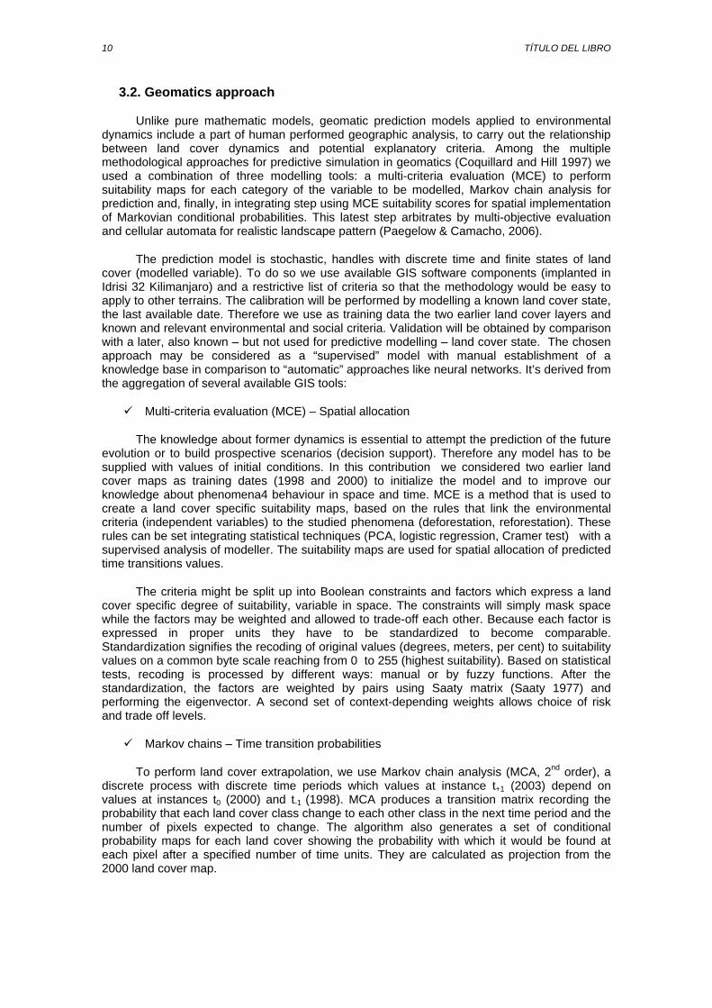
Unlike pure mathematic models, geomatic prediction models applied to environmental dynamics include a part of human performed geographic analysis, to carry out the relationship between land cover dynamics and potential explanatory criteria. Among the multiple methodological approaches for predictive simulation in geomatics (Coquillard and Hill 1997) we used a combination of three modelling tools: a multi-criteria evaluation (MCE) to perform suitability maps for each category of the variable to be modelled, Markov chain analysis for prediction and, finally, in integrating step using MCE suitability scores for spatial implementation of Markovian conditional probabilities. This latest step arbitrates by multi-objective evaluation and cellular automata for realistic landscape pattern (Paegelow & Camacho, 2006).

The prediction model is stochastic, handles with discrete time and finite states of land cover (modelled variable). To do so we use available GIS software components (implanted in Idrisi 32 Kilimanjaro) and a restrictive list of criteria so that the methodology would be easy to apply to other terrains. The calibration will be performed by modelling a known land cover state, the last available date. Therefore we use as training data the two earlier land cover layers and known and relevant environmental and social criteria. Validation will be obtained by comparison with a later, also known – but not used for predictive modelling – land cover state. The chosen approach may be considered as a “supervised” model with manual establishment of a knowledge base in comparison to “automatic” approaches like neural networks. It’s derived from the aggregation of several available GIS tools:

Multi-criteria evaluation (MCE) – Spatial allocation

The knowledge about former dynamics is essential to attempt the prediction of the future evolution or to build prospective scenarios (decision support). Therefore any model has to be supplied with values of initial conditions. In this contribution we considered two earlier land cover maps as training dates (1998 and 2000) to initialize the model and to improve our knowledge about phenomena4 behaviour in space and time. MCE is a method that is used to create a land cover specific suitability maps, based on the rules that link the environmental criteria (independent variables) to the studied phenomena (deforestation, reforestation). These rules can be set integrating statistical techniques (PCA, logistic regression, Cramer test) with a supervised analysis of modeller. The suitability maps are used for spatial allocation of predicted time transitions values.

The criteria might be split up into Boolean constraints and factors which express a land cover specific degree of suitability, variable in space. The constraints will simply mask space while the factors may be weighted and allowed to trade-off each other. Because each factor is expressed in proper units they have to be standardized to become comparable. Standardization signifies the recoding of original values (degrees, meters, per cent) to suitability values on a common byte scale reaching from 0 to 255 (highest suitability). Based on statistical tests, recoding is processed by different ways: manual or by fuzzy functions. After the standardization, the factors are weighted by pairs using Saaty matrix (Saaty 1977) and performing the eigenvector. A second set of context-depending weights allows choice of risk and trade off levels.

Markov chains – Time transition probabilities

To perform land cover extrapolation, we use Markov chain analysis (MCA, 2nd order), a discrete process with discrete time periods which values at instance t+1 (2003) depend on values at instances t0 (2000) and t-1 (1998). MCA produces a transition matrix recording the probability that each land cover class change to each other class in the next time period and the number of pixels expected to change. The algorithm also generates a set of conditional probability maps for each land cover showing the probability with which it would be found at each pixel after a specified number of time units. They are calculated as projection from the 2000 land cover map.

11

Integrating step based on multi-objective evaluation and cellular automata

The spatial allocation of predicted land cover time transition probabilities uses MCE performed suitability maps and a multi-objective evaluation (MOE) arbitrating between the set of finite land cover states. Finally we add an element of spatial contiguity by applying a cellular automaton (contiguity filter); it decreases the suitability of isolated pixel and favours the generation of more compacted patches. The algorithm is iterative so as to match with time distances between t-1 - t0 and between t0 - t+1.

3.3. Land Change Modeller approach

LCM is the new integrated modelling environment of Idrisi Andes for studying landscape trajectories and land use dynamics; it includes tools for analyzing the past land cover change, modelling the potential for future change, predicting the phenomena evolution, assessing its implication on biodiversity and ecological equilibrium and integrating planning regimes into predictions.

Land Cover Change analysis

The first step permits us to analyze the past land cover change between 1998 and 2000, chosen as training dates. We can easily calculate the gains and losses, the net change for each class (Fig ) and the surface trends for each transition.

Land Cover Change modelling

The land cover change modelling allows us to define 2 sub-model (forest to cleared areas=deforestation and cleared areas to forest=reforestation) and explore the explanatory power of environmental criteria (using the Cramer test). The quantitative variables can be included into the model either as static or dynamic factors; the static ones are unchanging over the time (e.g., distance from pipeline, distance from Rio San Pedro) and express the basic suitability for each transition. The dynamic variables change over the training and simulated period (distance of clearing areas, distance from developing roads) and are recalculated for each interaction during the course of prediction. Once the criteria were set, we calculated two transition potential maps using the Multi Layer Perceptron (MPL) neural networks. These express for each pixel the potential it has for both reforestation and deforestation. The MPL is more flexible than logistic regression procedure and allows one to model non-linear relationships. For the training process it creates a random sample of transition cell and a sample of persistent cells; it uses half the samples to train and to develop a multivariate function (adjusting the weights) that predicts the potential for change based on the value of environmental criteria at any location, and the second half of sample to test its performances (validation). The number of training pixels will affect the accuracy of the training result: a small sample size may not represent the population for each category, while too many samples may cause an over training of the network. We construct a network aggregating an Input layer with 10 neurons, an Hidden layer with 4 neurons and the Output layer with 2 neurons (suitability for deforestation and reforestation); we used a learning rate of 0.000121 and a momentum factor of 0,5 . After 5000 interaction we achieved an accuracy rate of approximately 87%. The next classification phase performs the Neural Network classification which produces the transition potential maps for deforestation and reforestation.

Land Cover Change Prediction

The quantity of change for each transition was calculated using the Markov Chains Analysis (MCA, above mentioned), from the 1998 and 2000 classified images and specifying the 2003 end date. We created both hard and soft maps; the first ones are definitive maps in which each pixel belongs to a certain class. The soft ones are a group of images showing the degree of membership of each pixel to each possible class and yield a map of vulnerability to deforestation, pointing out possible hot spots. We use 3 recalculation steps during which the dynamic variables are update. At the end we added the planning interventions tool, creating a disincentive for deforestation (1,5 multiplicative factor for southern areas) in the north side of

12 TÍTULO DEL LIBRO

Rio San Pedro ( affected by narcotraffic interests which limit the movement freedom; the roads in the southern part will be the main vector of penetration in this test area, replacing the Rio San Pedro) and an incentive for reforestation in central highlands (communitarian zone) where a nomad agriculture permits a more sustainable use of natural resources.

3.4. Dinamica EGO approach

Dinamica use a cellular automata approach to reproduce the landscape dynamics and the way its spatial patterns evolve. The simulation environment aggregates several steps which are easily built by connecting algorithms (functors) via their port, using a friendly graphical interface or XLM language. We resume here the main stages from calibration to validation of predicted Output and the adopted parameters:

Amount of change estimate

The first easy model allows calculating the amount of change for each transition through the Markov chains Analysis of second order (comparing two land use/cover map in different dates); we used the 1998 classified map as early image and 2000 map as last information for computing the transition matrix.

Weights of Evidence Method – Change allocation

A probability map of occurrence for each transition is produced using the Weight of Evidence (WOE) method. This is a Bayesian approach to highlight the relationships between environmental criteria and land use/ cover change. The favourability for one transition (e.g., deforestation D), given a binary map describing a spatial pattern C, can be expressed by the conditional probability:

P D |CR S

aP D T CR S

P CP Q

fffffffffffffffffffffffffffffffffa P D

P Q

P C | DR S

P CP Q

fffffffffffffffffffffffffff (4)

Algebraic manipulation allows representing this formula in terms of Logit (log odds) and Weights of Evidence (Bonham-Carter, 1994):

(5) Logit D | CR S

a logit DP QL W L

This method can be extended to handle multiple predictive maps and to relate a change with respect several geographical patterns; some restrictive hypothesis on analysed area and prior odds ratio for each transition will be necessary. At the end the conditional probability for deforestation, given a group of environmental criteria for each pixel, is expressed by:

f (6) P D |C1TC2TC3TCn

R S

aePW L

1L ePW Lffffffffffffffffffffffffffffff

The WOE model allows categorizing the continuous quantitative variables, evaluating the correlation of explanatory maps and displaying the weights of evidence with respect each environmental criteria. The Output is saved as text file.

Land Use/Cover Change prediction

The simulation model allows reproducing the spatial patterns evolution taking into account a large number of parameters specified in the used containers, such as:

Select percent Matrix: we express the percentage of pixels, for each transition, that will be modified using the Expander function; this process expands or contracts the previous

13

patches of certain class (e.g., previous cleared areas). The (1 – Expander %) percentage is treated with the Patcher function, which creates new patches through a seeding mechanism. We have chosen a percentage of 50% for deforestation and 70% for reforestation.

Select transition Parameter Matrix: this container take into account three parameters for Expander and Patcher functions. The mean patch size describe the mean size (hectares) of new pixels groups that will be modified for each transition; increasing this value leads to model a less fragmented landscape with large patches for every classes. The second parameter is the patch size variance, which determines how much the patch size can vary regarding the medium value; increasing this number leads to a more diverse landscape. Finally the isometry determines the degree of aggregation of the patches (values >1 permit a better cohesion of cells groups). We have chosen a mean size of 4 and 2 ha, a variance values of 2 and 1 ha and an isometry of 1,3 and 1,1, respectively for deforestation and reforestation.

4. Results

Four 2003 Land Cover maps were produced using the above-mentioned predictive models (Fig.5). We have semplified the complexity of land use/cover change only considering two transitions: deforestation and reforestation. The different simulation models were employed to projected future landscape evolution under the same scenario. A scenario describes possible future situation based on different hypotesis about socio-economic, demographic, political, ecological, etc., conditions (Hauglustaine et al.,2004; De Castro et al., 2007). We have drawn our scenario using the information observed in the last years of training period (1998-2000).

Fig 5: Outputs of predictive models

14 TÍTULO DEL LIBRO

5. Validation and discussion of results

To understand how well the models performed, many statistical methods measuring the agreement between two categorical maps have been developed in the last years. However they didn’t offer an exhaustive answer to validation problem, particularly to analyse the spatial allocation of disagreement. Our first approach is to perform a visual examination between the reference image (real 2003 land cover map) and the models Output; we can quickly obtain a general idea about model performance, highlighting possible strong incongruence in terms of quantity and location.

Fig 6: PPNET output vs. Real map in 2003

We can remark that the PNNET model underestimates the deforestation amount in the southern zone (Fig.6); the performance improves for the central and northern regions. The spatial allocation of cleared areas is quite realistic, but their form is sometime fragmented, probably due to frontier pixel approximation.

Fig 7: Geomatic model Output vs. Real map in 2003

15

The geomatics model improves the number of deforested pixels as regards to PNNET output; we remark an overestimation of cleared areas around the La Joyanca site (image centre) and a compact aggregation of the same ones in the southern and central zones (Fig.7).

Fig 8: LCM Output vs. Real map in 2003

The Land Cover Modeler produced the worse spatial distribution of cleared areas with several deforested spots scattered in the central region. Some of them present a low realistic structure with a concentric alternation of Forest-Milpa (Fig.8).

Fig 9: Dinamica Output vs. Real map in 2003

At the end we visually examine the Dinamica Ego Output; we point out an underestimation of deforestation in southern area and an overestimation in the northern one. The form of cleared spots is more realistic as regards to the other models output, especially nearby the La Joyanca site (Fig.9).

16 TÍTULO DEL LIBRO

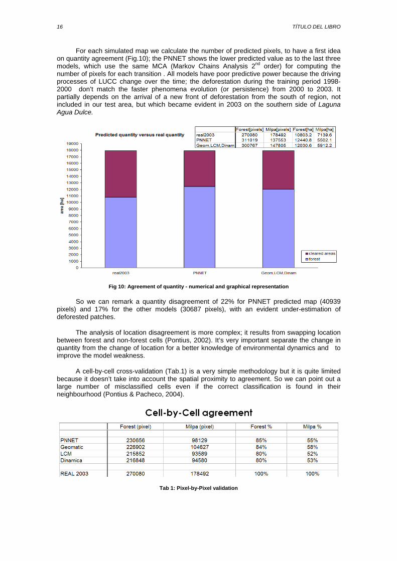
For each simulated map we calculate the number of predicted pixels, to have a first idea on quantity agreement (Fig.10); the PNNET shows the lower predicted value as to the last three models, which use the same MCA (Markov Chains Analysis 2nd order) for computing the number of pixels for each transition . All models have poor predictive power because the driving processes of LUCC change over the time; the deforestation during the training period 1998-2000 don’t match the faster phenomena evolution (or persistence) from 2000 to 2003. It partially depends on the arrival of a new front of deforestation from the south of region, not included in our test area, but which became evident in 2003 on the southern side of Laguna Agua Dulce.

Fig 10: Agreement of quantity - numerical and graphical representation

So we can remark a quantity disagreement of 22% for PNNET predicted map (40939 pixels) and 17% for the other models (30687 pixels), with an evident under-estimation of deforested patches.

The analysis of location disagreement is more complex; it results from swapping location between forest and non-forest cells (Pontius, 2002). It’s very important separate the change in quantity from the change of location for a better knowledge of environmental dynamics and to improve the model weakness.

A cell-by-cell cross-validation (Tab.1) is a very simple methodology but it is quite limited because it doesn’t take into account the spatial proximity to agreement. So we can point out a large number of misclassified cells even if the correct classification is found in their neighbourhood (Pontius & Pacheco, 2004).

Tab 1: Pixel-by-Pixel validation

17

The cell-by-cell validation highlights that all models present a poor performance for the Milpa with a medium value of 54.5% of agreement; this percentage increase for the Forest class to 82.25%. Considering this table we can conclude that the Geomatic model performs better for deforested patches (58%) and the PNNET for the forest prediction (85%).

We calculated now the LUCC budget (Tab.2) to point out the gains and loss for each category (we only consider the Milpa class because the map is binary) and the amount of changes from 2000 to 2003, as regard to real dynamics.

Tab 2: LUCC budget

For real evolution of deforestation (real 2000 x real 2003) we can remark an important total change (29%) which doesn’t appear in the LUCC-budget of 2003 simulated situations. In particular PNNET shows the lower value (10%), due to the absence of reforestation dynamic from 2000 to 2003 (0% loss for Milpa or, if you prefer, 0% forest gain); PNNET only predicts the evolution of clearing processes considering that there will be not forest regrowth in the old deforested patches. Dinamica performs the higher value for total change (18%) and a ratio Swap/Net-change (0.46) close to the real one (0.51), showing the best land cover dynamics approximation. The other models, particularly the neural networks, underestimate the land cover change, predicting the persistence.

We intersect now the simulated land cover maps and the real one, to point out the consistency between models (Tab.3). The correctly predicted area by the four models is about 53% which represents a poor consistency, against an individual prediction rate of about 70%. For each intersection the forest prediction is better than the Milpa one, due to the persistence and large area of this category in opposition to the fast and fragmented evolution of clearing phenomena. The best three models combination is the PNNET-Geomatic model-LCM, with an improvement rate of 6.25%; when we separately use the PNNET or Geomatic model with the other ones, we obtain a poor improvement. This consideration is remarked during subsequent analysis, where the higher value (13.57%) is obtained by the intersection between the PNNET and Geomatic model, indicating a good consistency. The lower improvement is done by the LCM and Dinamica (4.83%). Finally we analyze the contribution of single simulated output; we remark that the Geomatic model performs the best prediction (74%) followed by the PNNET (72.2%) with an improvement of about 21%. The last one shows a better ability in forest prediction (85.4% of real forest), while the Geomatic model performs better for the Milpa (58.62% of real disturbance).

We have seen that for each model, the correct prediction score is linked to the nature of the classes and to their spatial patterns evolution. We have remarked that the PNNET performs better for forest prediction and Geomatic model for Milpa prediction. Now we prove as these performances depend on the number of land cover change between 1998-2000-2003 (Fig.11). The neural network show the higher prediction score (93%) on the areas with land cover persistence (mainly closed forest areas), but it has the lower value for the more dynamic patches. The Geomatic model and Dinamica perform better for the zones with 1 or 2 land cover changes (mainly cleared areas with partial forest regrowth). All models show a good ability for persistence prediction driven by the simplicity of this phenomenon; unfortunately our attention is

18 TÍTULO DEL LIBRO

focused on deforestation processes which are more complex and interdependent on several factors. The models perform similarly on the areas which changed one time (only 50% of real amount) but we have a strong difference in model behaviour when land cover changes become more numerous, with a better prediction scores for Geomatic model (23%) and Dinamica (21%). We remark that these values are very small as regards to real amount of change.

Tab 3: Prediction rates by crossing the models Outputs

Fig 11: Prediction scores depending on the number of Land Cover Change – graph and table

19

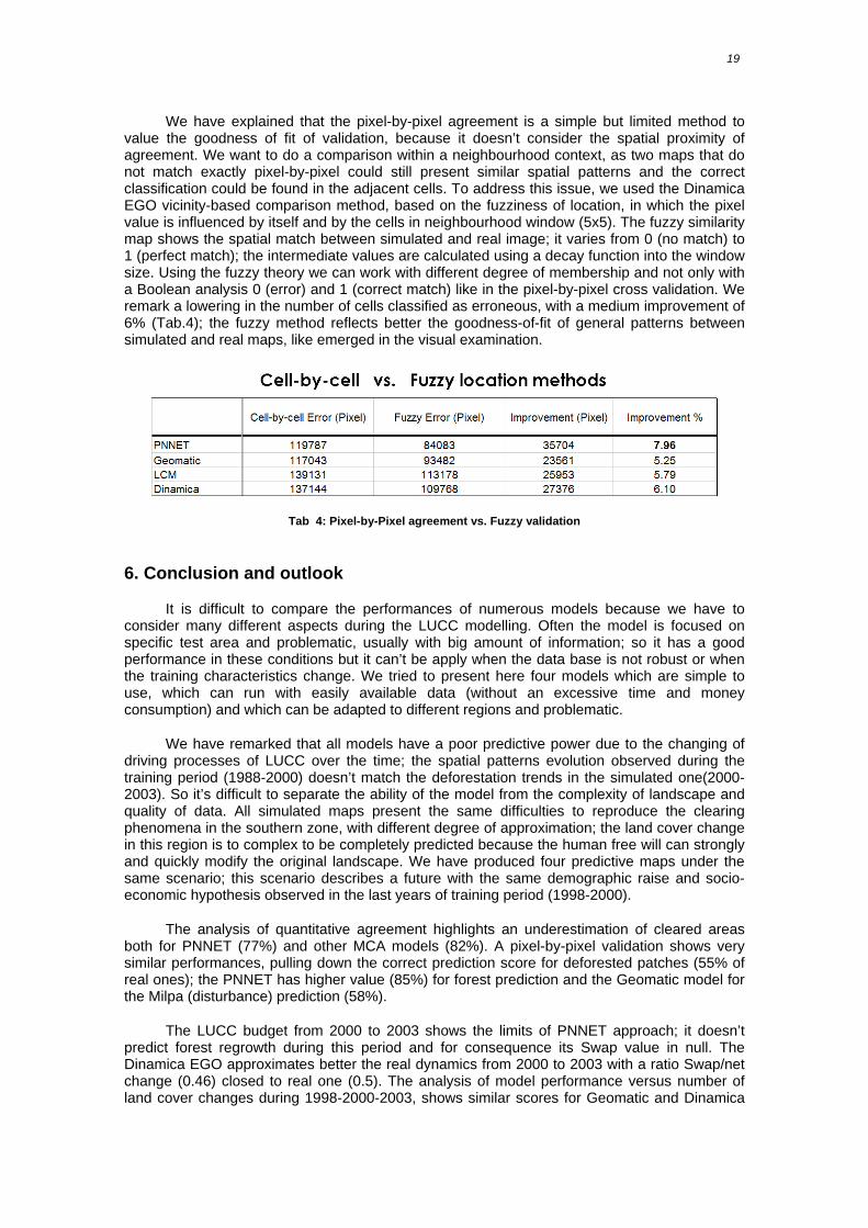
We have explained that the pixel-by-pixel agreement is a simple but limited method to value the goodness of fit of validation, because it doesn’t consider the spatial proximity of agreement. We want to do a comparison within a neighbourhood context, as two maps that do not match exactly pixel-by-pixel could still present similar spatial patterns and the correct classification could be found in the adjacent cells. To address this issue, we used the Dinamica EGO vicinity-based comparison method, based on the fuzziness of location, in which the pixel value is influenced by itself and by the cells in neighbourhood window (5x5). The fuzzy similarity map shows the spatial match between simulated and real image; it varies from 0 (no match) to 1 (perfect match); the intermediate values are calculated using a decay function into the window size. Using the fuzzy theory we can work with different degree of membership and not only with a Boolean analysis 0 (error) and 1 (correct match) like in the pixel-by-pixel cross validation. We remark a lowering in the number of cells classified as erroneous, with a medium improvement of 6% (Tab.4); the fuzzy method reflects better the goodness-of-fit of general patterns between simulated and real maps, like emerged in the visual examination.

Tab 4: Pixel-by-Pixel agreement vs. Fuzzy validation

6. Conclusion and outlook

It is difficult to compare the performances of numerous models because we have to consider many different aspects during the LUCC modelling. Often the model is focused on specific test area and problematic, usually with big amount of information; so it has a good performance in these conditions but it can’t be apply when the data base is not robust or when the training characteristics change. We tried to present here four models which are simple to use, which can run with easily available data (without an excessive time and money consumption) and which can be adapted to different regions and problematic.

We have remarked that all models have a poor predictive power due to the changing of driving processes of LUCC over the time; the spatial patterns evolution observed during the training period (1988-2000) doesn’t match the deforestation trends in the simulated one(2000-2003). So it’s difficult to separate the ability of the model from the complexity of landscape and quality of data. All simulated maps present the same difficulties to reproduce the clearing phenomena in the southern zone, with different degree of approximation; the land cover change in this region is to complex to be completely predicted because the human free will can strongly and quickly modify the original landscape. We have produced four predictive maps under the same scenario; this scenario describes a future with the same demographic raise and socio-economic hypothesis observed in the last years of training period (1998-2000).

The analysis of quantitative agreement highlights an underestimation of cleared areas both for PNNET (77%) and other MCA models (82%). A pixel-by-pixel validation shows very similar performances, pulling down the correct prediction score for deforested patches (55% of real ones); the PNNET has higher value (85%) for forest prediction and the Geomatic model for the Milpa (disturbance) prediction (58%).

The LUCC budget from 2000 to 2003 shows the limits of PNNET approach; it doesn’t predict forest regrowth during this period and for consequence its Swap value in null. The Dinamica EGO approximates better the real dynamics from 2000 to 2003 with a ratio Swap/net change (0.46) closed to real one (0.5). The analysis of model performance versus number of land cover changes during 1998-2000-2003, shows similar scores for Geomatic and Dinamica

20 TÍTULO DEL LIBRO

models, which have the best predictive power on the more dynamic areas (numerous changes), while PNNET performs better for persistent forest zones.

This contribution wants to point out the potentialities of predictive modelling for integrating the traditional approaches to environmental and hazard problems. Parallelly we want to remark that the model performance and utility depend on our geo-system knowledge and on the quality of data, often more than on the model conceptual foundation. The objectives will be clear to address an exhaustive answer: do we want to better know the observed object or to understand the long term effects of specific government planning or industrial project? Taking in account its goals, the modeller often prefer to work in simplified environment with very uniform dynamics and clear relationships; it’s an ideal situation to run a model and perform a good result, but its utility is quite limited. When we analyse a complex phenomena evolution we have to consider all interconnections between the natural and artificial dynamics; the early raw model Output could be quite poor but it helps us to improve our knowledge of hidden relationships between the studied phenomena and the key variables. The subsequent simulation will be better considering these new information.

The spatiotemporal models are simplified representations of reality. Represent is also re-represent, represent again, after a selected period; we have to accept that this result will be not an exact copy of reality. The re-representation has its own legitimacy: it has memory and project; it bases its legitimacy on the coherence with the past history and the future goals (La Moigne, 1994).

Acknowledges

The authors thank the project ?????-Selleron for the SPOT images availability.

References [1] Arnauld 2000

[2] Arrow 1974

[3] Atkinson 2003

[4] Bonham-Carter 1994

[5] Bruno, R., Follador, M., Paegelow, M., Renno, F., Villa, N., 2006

[6] Coquillard,P., and Hill,D.R.C., Modélisation et Simulation d’Ecosystemes. MASSON, Paris Milan Barcelone, 1997.

[7] Cruz 1976

[8] De Castro, F.V.F., Soares Filho, B.S., Mendoza, E., «Modelagem de cenarios de mudanças na região de Brasiléia aplicada ao Zoneamento Ecologico Economico do estado do Acre», Anais XIII Simposio Brasileiro de Sensoriamento Remoto, INPE, 5135-5142, 2007.

[9] Effantin-Touyer, R., De la frontière agraire à la frontière de la nature. Thése ECOLE DOCTORALE A.B.I.E.S, Paris, 2006.

[10] Follador M., Renno, F., 2005

[11] Geoghean 2001

[12] Hauglustaine, D., Jouzel, J., Le Treut, H., Climat: chronique d’un bouleversement annoncé. Le Pommier, Paris, 2005.

[13] Hengl, T., «Finding the right pixel size», Computer&Geosciences, 32,??,2006.

[14] Joshi, C., De Leeuw, J., Skidmore, A.K., van Duren, I.C, van Oosten, H., «Remotely sensed estimation of forest canopy density: A comparison of the performance of four methods», International Journal of Applied Earth Observation and Geoinformation, 8, 84-95, 2006.

21

[15] Kavouras 2001

[16] La Moigne, J.L., La Theorie du Systeme General. Puf, 1994.

[17] Lee, V.C.S, Wong,H.T., « A multivariate neuro-fuzzy system for foreign currency risk management decision making», Neurocomputing, 70, 942-951, 2007.

[18] Moore 1993

[19] Pontius, R.G.J, « Statistical Methodc to Partition Effects of Quantity and Location during Comparison of Categorical Maps at Multiple Resolutions», Photogrammetric Engineering & Remote Sensing, 10, 1041-1049, 2002.

[20] Pontius, R.G.J. and Pacheco,P., «Calibration and validation of a model of forest disturbance in the Western Ghats, India 1920–1990», GeoJournal, 61, 325-334, 2004.

[21] Pontius, R.G.J. and Chen, «Land Use and Cover Change Modellin» 2006

[22] Paegelow, M. and Camacho 2006

[23] Rodrigues, H.O., Soares-Filho, B.S., de Souza Costa, W.L., «Dinamica EGO, uma plataforma para modelagem de sistemas ambientais»

[24] Saaty, T.L., « A Scaling Method for Priorities in Hierarchical Structures », J. Math. Psychology, 15, 234-28, 1977.

[25] Villa, N., 2007

[26] Venables, Ripley 1999

Graphics must be placed in text and be attached in file apart in JPG format.

Los gráficos deben situarse en el texto y adjuntarse en fichero aparte en formato JPG.

Les graphiques doivent se situer dans le texte et dans un fichier à part avec format JPG.