TROPICAL ALGEBRAIC GEOMETRY

ANDREAS GATHMANN

There are many examples in algebraic geometry in which complicated geometric or algebraic problemscan be transformed into purely combinatorial problems. The most prominent example is probably givenby toric varieties — a certain class of varieties that can be described purely by combinatorial data, e.g. bygiving a convex polytope in an integral lattice. As a consequence, most questions about these varietiescan be transformed into combinatorial questions on the defining polytope that are then hopefully easierto solve.

Tropical algebraic geometry is a recent development in the field of algebraic geometry that tries togeneralize this idea substantially. Ideally, every construction in algebraic geometry should have a com-binatorial counterpart in tropical geometry. One may thus hope to obtain results in algebraic geometryby looking at the tropical (i.e. combinatorial) picture first and then trying to transfer the results back tothe original algebro-geometric setting.

The origins of tropical geometry date back about twenty years. One of the pioneers of the theory wasImre Simon [Si], a mathematician and computer scientist from Brazil — which is by the way the onlyreason for the peculiar name “tropical geometry”. Originally, the theory was developed in an appliedcontext of discrete mathematics and optimization, but it has not been part of the mainstream in eitherof mathematics, computer science or engineering. Only in the last few years have people realized itspower for applications in fields such as combinatorics, computational algebra, and algebraic geometry.

This is also why the theory of tropical algebraic geometry is still very much in its beginnings: not eventhe concept of a variety has been defined yet in tropical geometry in a general and satisfactory way. Onthe other hand there are already many results in tropical geometry that show the power of these newmethods. For example, Mikhalkin has proven recently that tropical geometry can be used to computethe numbers of plane curves of given genus g and degree d through 3d +g−1 general points [M1] —a deep result that had been obtained first by Caporaso and Harris about ten years ago by a complicatedstudy of moduli spaces of plane curves [CH].

In this expository article we will for simplicity restrict ourselves mainly to the well-established theoryof tropical plane curves. Even in this special case there are several seemingly different approaches tothe theory. We will describe these approaches in turn in chapter 1 and discuss possible generalizationsat the end. We will then explain in chapter 2 how some well-known results from classical geometry —e.g. the degree-genus formula and Bezout’s theorem — can be recovered (and reproven) in the languageof tropical geometry. Finally, in chapter 3 we will discuss the most powerful applications of tropicalgeometry known so far, namely to complex and real enumerative geometry.

1. PLANE TROPICAL CURVES

1.1. Tropical curves as limits of amoebas. With classical (complex) algebraic geometry in mind themost straightforward way to tropical geometry is via so-called amoebas of algebraic varieties. Fora complex plane curve C the idea is simply to restrict it to the open subset (C∗)2 of the (affine orprojective) plane and then to map it to the real plane by the map

Log : (C∗)2→ R2

z = (z1,z2) 7→ (x1,x2) := (log |z1|, log |z2|).1

2 ANDREAS GATHMANN

The resulting subset A = Log(C∩ (C∗)2) of R2 is called the amoeba of the given curve. It is of coursea two-dimensional subset of R2 since complex curves are real two-dimensional. The following pictureshows three examples (where we set e := exp(1)):

x1

x2

x1 x1

x2x2

(c) C = a generic conic

A A

(a) C = {z; z1 + z2 = 1}

−2

−3

A

(b) C = {z; e3z1 + e2z2 = 1}

FIGURE 1. Three amoebas of plane curves

In fact, the shape of these pictures (that also explains the name “amoeba”) can easily be explained. Incase (a) for example the curve C contains exactly one point whose z1-coordinate is zero, namely (0,1).As log0 =−∞ a small neighborhood of this point is mapped by Log to the “tentacle” of the amoeba Apointing to the left. In the same way a neighborhood of (1,0) ∈C leads to the tentacle pointing down,and points of the form (z,1− z) with |z| → ∞ to the tentacle pointing to the upper right.

In case (b) the multiplicative change in the variable simply leads to an (additive) shift of the amoeba. In(c) a generic conic, i.e. a curve given by a general polynomial of degree 2, has two points each whereit meets the coordinate axes, leading to two tentacles in each of the three directions. In the same wayone could consider curves of an arbitrary degree d that would give us amoebas with d tentacles in eachdirection.

To make these amoebas into combinatorial objects the idea is simply to shrink them to “zero width”. Soinstead of the map Log above let us consider the maps

Logt : (C∗)2→ R2

(z1,z2) 7→ (− logt |z1|,− logt |z2|) =(− log |z1|

log t,− log |z2|

log t

)for small t ∈ R and study the limit of the amoebas Logt(C∩ (C∗)2) as t tends to zero. As Logt differsfrom Log only by a rescaling of the two axes the result for the curve in figure 1 (a) is the graph Γ shownin the following picture on the left. We call Γ the tropical curve determined by C.

x1

x2

x1 x1

x2x2

(a) C = {z; z1 + z2 = 1}

Γ ΓΓ

−2

−3

(c) Ct : a family of conics(b) Ct = {z; t−3z1 + t−2z2 = 1}

FIGURE 2. The tropical curves corresponding to the amoebas in figure 1

TROPICAL ALGEBRAIC GEOMETRY 3

If we did the same thing with the curve (b) the result would of course be that we not only shrink theamoeba to zero width, but also move its “vertex” to the origin, leading to the same tropical curve asin (a). To avoid this we consider not only one curve C = {z; e3z1 + e2z2 = 1} but the family of curvesCt = {z; t−3z1 + t−2z2 = 1} for small t ∈ R. This family has the property that Ct passes through (0, t2)and (t3,0) for all t, and hence all Logt(Ct ∩(C∗)2) have their horizontal and vertical tentacles at z2 =−2and z1 = −3, respectively. So if we now take the limit as t → 0 we shrink the width of the amoeba tozero but keep its position in the plane: we get the shifted tropical curve as in figure 2 (b). We call thisthe tropical curve determined by the family (Ct).

For (c) we can proceed in the same way: using a suitable family of conics we can shrink the width ofthe amoeba A to zero while keeping the position of its tentacles fixed. The resulting tropical curve Γ,i.e. the limit of Logt(Ct ∩ (C∗)2), may e.g. look like in figure 2 (c). We will see at the end of section 1.4however that this is not the only type of graph that we can obtain by a family of conics in this way.

Summarizing we can say informally that a tropical curve should be a subset of R2 obtained as the limit(in a certain sense) of the amoebas Logt(Ct ∩ (C∗)2), where (Ct) is a suitable family of plane algebraiccurves. They are all piecewise linear graphs with certain properties that we will study later.

1.2. Tropical curves via varieties over the field of Puiseux series. Of course this method of con-structing (or even defining) tropical curves is very cumbersome as it always involves a limiting processover a whole family of complex curves. There is an elegant way to hide this limiting process by replac-ing the ground field C by the field K of so-called Puiseux series, i.e. the field of formal power seriesa = ∑q∈Q aqtq in a variable t such that the subset of Q of all q with aq 6= 0 is bounded below and has afinite set of denominators. For such an a ∈ K with a 6= 0 the infimum of all q with aq 6= 0 is actually aminimum; it is called the valuation of a and denoted vala.

Using this construction we can say for example that our family (b) in section 1.1

C = {z ∈ K2; t−3z1 + t−2z2 = 1} ⊂ K2

now defines one single curve in the affine plane over this new field K. How do we now perform the limitt → 0 in this set-up? For an element a = ∑q∈Q aqtq ∈ K only the term with the smallest exponent, i.e.avalatvala, will be relevant in this limit. So applying the map logt we get for small t

logt |a| ≈ logt |avalatvala|= vala+ logt |avala| ≈ vala.

In our new picture the operations of applying the map Logt and taking the limit for t → 0 thereforecorrespond to the map

Val : (K∗)2→ R2

(z1,z2) 7→ (x1,x2) := (−valz1,−valz2).

Using this observation we can now give our first rigorous definition of plane tropical curves:

Definition A. A plane tropical curve is a subset of R2 of the form Val(C∩ (K∗)2), where C is a planealgebraic curve in K2. (Strictly speaking we should take the closure of Val(C∩ (K∗)2) in R2 since theimage of the valuation map Val is by definition contained in Q2.)

Note that this definition is now purely algebraic and does not involve any limit taking processes. AsK is an algebraically closed field of characteristic zero (in fact it is the algebraic closure of the field ofLaurent series in t) the theory of algebraic geometry of plane curves over K is largely identical to thatof algebraic curves over C.

As an example let us consider again case (b) of section 1.1, i.e. the curve C ⊂ K2 given by the equationt−3z1 + t−2z2 = 1. If (z1,z2) ∈C∩ (K∗)2 then Val(z1,z2) can give three different kinds of results:

• If valz1 > 3 then the valuation of z2 = t2− t−1z1 is 2 since all exponents of t in t−1z1 are biggerthan 2. Hence these points map precisely to the left edge of the tropical curve in figure 2 (b)under Val.• In the same way we get the bottom edge of this tropical curve if valz2 > 2.

4 ANDREAS GATHMANN

• If valz1 ≤ 3 and valz2 ≤ 2 then the equation t−3z1 + t−2z2 = 1 shows that the leading terms oft−3z1 and t−2z2 must have the same valuation, i.e. that valz1 = valz2+1. This leads to the upperright edge of the tropical curve in figure 2 (b).

So we recover our old result, i.e. the tropical curve drawn in figure 2 (b).

One special case is worth mentioning: if the curve C⊂K2 is given by an equation whose coefficients liein C (i.e. are “independent of t”) then for any point (z1(t),z2(t)) ∈C the points (z1(tq),z2(tq)) for q ∈Qare obviously in C as well. As replacing t by tq for some q > 0 simply multiplies the valuation with q weconclude that the tropical variety associated to C in this case is a cone (i.e. a union of half-rays startingat the origin) — as it was the case e.g. in figure 2 (a).

1.3. Tropical curves as varieties over the max-plus semiring. We now want to study definition A inmore detail. Let C ⊂ K2 be a plane algebraic curve given by the polynomial equation

C =

{(z1,z2) ∈ K2; f (z1,z2) := ∑

i, j∈Nai jzi

1z j2 = 0

}for some ai j ∈ K of which only finitely many are non-zero. Note that the valuation of a summand off (z1,z2) is

val(ai jzi1z j

2) = valai j + ivalz1 + j valz2.

Now if (z1,z2) is a point of C then all these summands add up to zero. In particular, the lowest valuationof these summands must occur at least twice since otherwise the corresponding terms in the sum couldnot cancel. For the corresponding point (x1,x2) = Val(z1,z2) = (−valz1,−valz2) of the tropical curvethis obviously means that in the expression

g(x1,x2) := max{ix1 + jx2−valai j; (i, j) ∈ N2 with ai j 6= 0} (∗)the maximum is taken on at least twice. It follows that the tropical curve determined by C is containedin the “corner locus” of this convex piecewise linear function g, i.e. in the locus where this function isnot differentiable. In fact, Kapranov’s theorem states that the converse inclusion holds as well, i.e. thatthe tropical curve determined by C is precisely this corner locus (see e.g. [K], [Sh]).

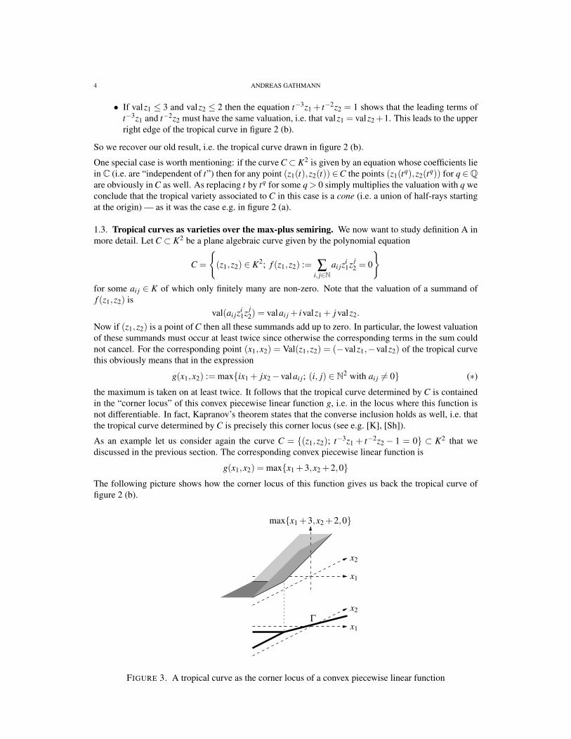
As an example let us consider again the curve C = {(z1,z2); t−3z1 + t−2z2 − 1 = 0} ⊂ K2 that wediscussed in the previous section. The corresponding convex piecewise linear function is

g(x1,x2) = max{x1 +3,x2 +2,0}The following picture shows how the corner locus of this function gives us back the tropical curve offigure 2 (b).

x1

x1

x2

x2

max{x1 +3,x2 +2,0}

Γ

FIGURE 3. A tropical curve as the corner locus of a convex piecewise linear function

TROPICAL ALGEBRAIC GEOMETRY 5

These convex piecewise linear functions are often written in a different way in order to resemble thenotation of the original polynomial: for two real numbers x,y we define “tropical addition” and “tropicalmultiplication” simply by

x⊕ y := max{x,y} and x� y := x+ y.

The real numbers together with these two operations form a semiring, i.e. they satisfy all propertiesof a ring except for the existence of additive neutral and inverse elements. Sometimes an element−∞ is formally added to the real numbers to serve as a neutral element, but there is certainly no way toconstruct inverse elements as this would require equations of the form max{−∞,x}=−∞ to be solvable.

Using this notation we can write our convex piecewise linear function (∗) above as

g(x1,x2) =⊕i, j

(−valai j)� x�i1 � x� j

2 .

We call this expression the tropicalization of the original polynomial f . It can be considered as a“tropical polynomial”, i.e. as a polynomial in the tropical semiring. For example, the tropicalization ofthe polynomial t−3z1 + t−2z2−1 is just

3� x1⊕2� x2⊕0 = max{x1 +3,x2 +2,0}.(Note that the addition of 0 is not superfluous here since 0 is not a neutral element for tropical addition!)

We can therefore now give an alternative definition of plane tropical curves that does not involve thesomewhat complicated field of Puiseux series any more:

Definition B. A plane tropical curve is a subset of R2 that is the corner locus of a tropical polynomial,i.e. of a polynomial in the tropical semiring (R,⊕,�) = (R,max,+).

Again there is a special case that is completely analogous to the one mentioned at the end of section 1.2:if the tropical polynomial g is the maximum of linear functions without constant terms (e.g. because itis the tropicalization of a polynomial with coefficients that do not depend on t) then the corner locus ofg is a cone. If this is not the case and g is the maximum of many affine functions then its corner locuswill in general be a complicated piecewise linear graph in the plane as e.g. in figure 2 (c).

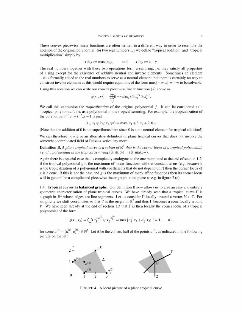
1.4. Tropical curves as balanced graphs. Our definition B now allows us to give an easy and entirelygeometric characterization of plane tropical curves. We have already seen that a tropical curve Γ isa graph in R2 whose edges are line segments. Let us consider Γ locally around a vertex V ∈ Γ. Forsimplicity we shift coordinates so that V is the origin in R2 and thus Γ becomes a cone locally aroundV . We have seen already at the end of section 1.3 that Γ is then locally the corner locus of a tropicalpolynomial of the form

g(x1,x2) =⊕

i

x�a(i)11 � x

�a(i)22 = max{a(i)1 x1 +a(i)2 x2; i = 1, . . . ,n}.

for some a(i) = (a(i)1 ,a(i)2 ) ∈N2. Let ∆ be the convex hull of the points a(i), as indicated in the followingpicture on the left:

1 32

1

2

∆

a(1)

a(2)a(5)

a(3)

a(4)

V

Γ

20

FIGURE 4. A local picture of a plane tropical curve

6 ANDREAS GATHMANN

First of all we claim that any point a(i) that is not a vertex of ∆ is irrelevant for the tropical curve Γ. Infact, it is impossible for such an a(i) (as e.g. a(5) in the example above) that the expression a(i)1 x1+a(i)2 x2

is strictly bigger than all the other a( j)1 x1 + a( j)

2 x2 for some x1,x2 ∈ R. Hence g and therefore also itscorner locus remain the same if we drop this term. In particular we see that — unlike in classicalalgebraic geometry — there is no hope for a one-to-one correspondence between tropical curves andtropical polynomials (up to scalars).

It is now easy to see that the corner locus of g consists precisely of those points where

g(x1,x2) = a(i)1 x1 +a(i)2 x2 = a( j)1 x1 +a( j)

2 x2

for two adjacent vertices a(i) and a( j) of ∆. An easy computation shows that for fixed i and j this isprecisely the half-ray starting from the origin and pointing in the direction of the outward normal of theedge joining a(i) and a( j). So as shown in figure 4 on the right the tropical curve Γ is simply the unionof all these outward normal lines locally around V . In particular all edges of Γ have rational slopes.

There is one more important condition on the edges of Γ around V that follows from this observation.If a(1), . . . ,a(n) are the vertices of ∆ in clockwise direction then an outward normal vector of the edgejoining a(i) and a(i+1) (where we set a(n+1) := a(1)) is v(i) :=(a(i)2 −a(i+1)

2 ,a(i+1)1 −a(i)1 ) for all i= 1, . . . ,n.

In particular it follows that ∑ni=1 v(i) = 0. This fact is usually expressed as follows: we write the vectors

v(i) as v(i) = w(i) · u(i) where u(i) is the primitive integral vector in the direction of v(i) and w(i) ∈ N>0.We call w(i) the weight of the corresponding edge of Γ and thus consider Γ to be a weighted graph.Our equation ∑i v(i) = 0 then states that the weighted sum of the primitive integral vectors of the edgesaround every vertex of Γ is 0. This is usually called the balancing condition. For example, in figure 4the edge of Γ pointing down has weight 2 (since v(2) = (0,−2) = 2 · (0,−1)), whereas all other edgeshave weight 1. In this paper we will usually label the edges with their corresponding weights unlessthese weights are 1. The balancing condition around the vertex V then reads

(2,1)+2 · (0,−1)+(−1,−1)+(−1,2) = (0,0)

in this example.

Together with our observation of section 1.1 that (at least generic) plane algebraic curves of degree dlead to plane tropical curves with d ends each in the directions (−1,0), (0,−1), and (1,1), we arrive atthe following somewhat longer but purely geometric definition of plane tropical curves:

Definition C. A plane tropical curve of degree d is a weighted graph Γ in R2 such that

(a) every edge of Γ is a line segment with rational slope;(b) Γ has d ends each in the directions (−1,0), (0,−1), and (1,1) (where an end of weight w counts

w times);(c) at every vertex V of Γ the balancing condition holds: the weighted sum of the primitive integral

vectors of the edges around V is zero.

Strictly speaking we have only explained above why a plane tropical curve in the sense of definition Bgives rise to a curve in the sense of definition C. One can show that the converse holds as well; a proofcan e.g. be found in [M1] or [Sp] chapter 5.

With this definition it has now become a combinatorial problem to find all types of plane tropical curvesof a given degree. In fact, the construction given above globalizes well: assume that Γ is the tropicalcurve given as the corner locus of the tropical polynomial

g(x1,x2) = max{a(i)1 x1 +a(i)2 x2 +b(i); i = 1, . . . ,n}.

If g is the tropicalization of a polynomial of degree d then the a(i) are all integer points in the triangle∆d := {(a1,a2); a1 ≥ 0,a2 ≥ 0,a1 + a2 ≤ d}. Consider two terms i, j ∈ {1, . . . ,n} with a(i) 6= a( j). Ifthere is a point (x1,x2) ∈ R2 such that

g(x1,x2) = a(i)1 x1 +a(i)2 x2 +b(i) = a( j)1 x1 +a( j)

2 x2 +b( j)

TROPICAL ALGEBRAIC GEOMETRY 7

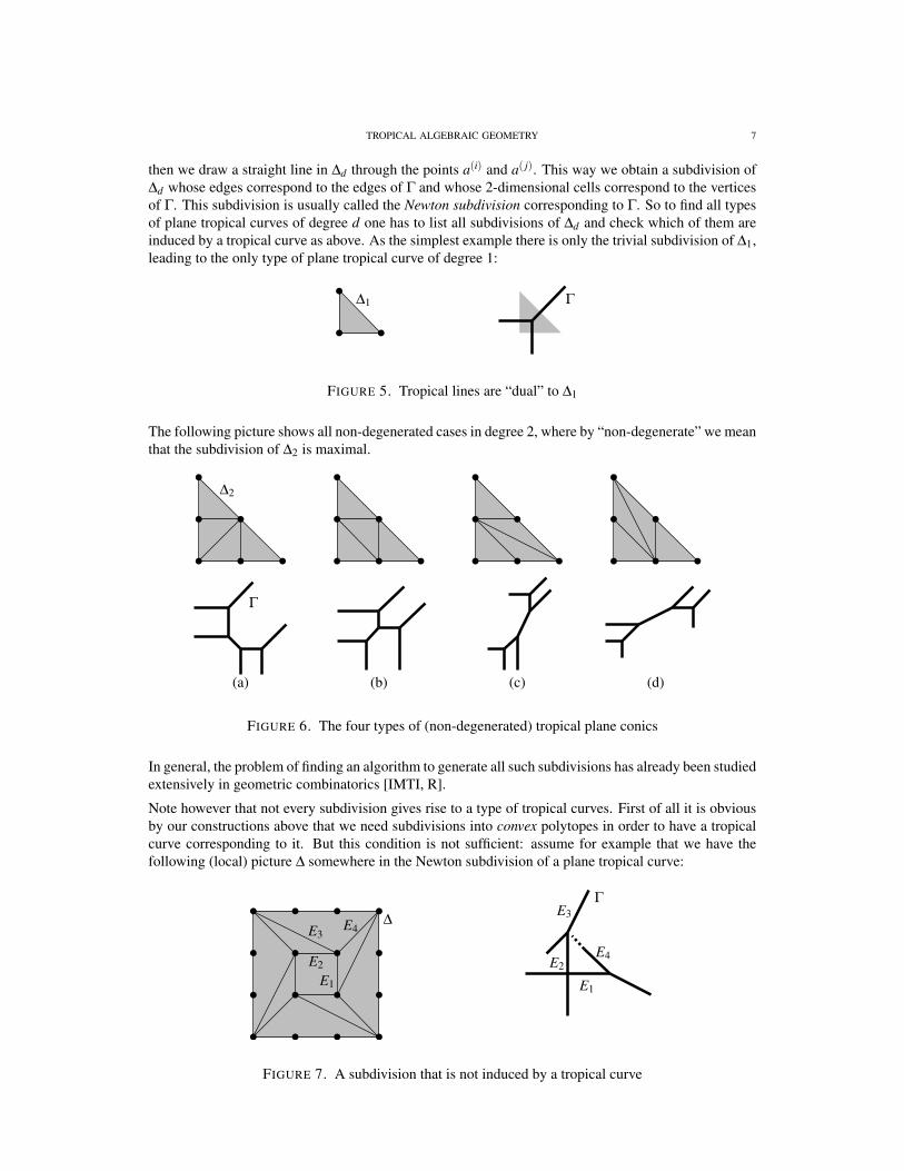
then we draw a straight line in ∆d through the points a(i) and a( j). This way we obtain a subdivision of∆d whose edges correspond to the edges of Γ and whose 2-dimensional cells correspond to the verticesof Γ. This subdivision is usually called the Newton subdivision corresponding to Γ. So to find all typesof plane tropical curves of degree d one has to list all subdivisions of ∆d and check which of them areinduced by a tropical curve as above. As the simplest example there is only the trivial subdivision of ∆1,leading to the only type of plane tropical curve of degree 1:

∆1 Γ

FIGURE 5. Tropical lines are “dual” to ∆1

The following picture shows all non-degenerated cases in degree 2, where by “non-degenerate” we meanthat the subdivision of ∆2 is maximal.

Γ

(a) (b) (c) (d)

∆2

FIGURE 6. The four types of (non-degenerated) tropical plane conics

In general, the problem of finding an algorithm to generate all such subdivisions has already been studiedextensively in geometric combinatorics [IMTI, R].

Note however that not every subdivision gives rise to a type of tropical curves. First of all it is obviousby our constructions above that we need subdivisions into convex polytopes in order to have a tropicalcurve corresponding to it. But this condition is not sufficient: assume for example that we have thefollowing (local) picture ∆ somewhere in the Newton subdivision of a plane tropical curve:

∆

Γ

E1

E2

E3

E4E2

E1

E4E3

FIGURE 7. A subdivision that is not induced by a tropical curve

8 ANDREAS GATHMANN

In the tropical curve Γ that would correspond to this subdivision the edge E4 would have to meet E3 andnot E2 at the dotted end, so E2 must be longer than E1. But the same argument can be used cyclicallyto conclude that each edge around the central vertex must be longer than the previous one. As this isnot possible we conclude that there cannot be a tropical curve corresponding to this subdivision of ∆.In fact, the subdivisions corresponding to tropical curves are precisely the ones that are usually calledthe regular polyhedral subdivisions, i.e. the ones that can be written as the corner locus of a piecewiselinear convex function similarly to figure 3.

It should also be stressed that the subdivision of ∆d determines only the combinatorial type of thetropical curve and not the curve itself. For example, each of the types in figure 6 describes a (real)5-dimensional family of plane tropical conics since the lengths of the bounded edges (3 parameters) aswell as the position in the plane (2 parameters) can vary arbitrarily. Note that this agrees nicely with theclassical picture: conics in the complex plane vary in a 5-dimensional family as well (corresponding tothe 6 coefficients of a quadratic equation modulo a common scalar).

1.5. Generalizations. At the end of this chapter let us briefly describe how the theory of plane tropicalcurves given above can be generalized.

First of all it is quite obvious to note that essentially the same constructions and the same theory can becarried through for curves that are not necessarily in the plane but in any toric surface, i.e. in any surfaceX with a C∗-action that contains (C∗)2 as a dense open subset. Definition A remains unchanged in thiscase; the resulting tropical curves will still be graphs in R2. Definition B only has to be modified as toallow Laurent polynomials compatible with the chosen homology class of the curves; and in definitionC the only change is in the directions of the ends of Γ. In fact, a toric surface X together with a positivehomology class corresponds exactly to a convex integral polytope ∆, and the types of tropical curvescoming from this homology class are precisely those determined by subdivisions of ∆ as explained atthe end of section 1.4.

In the same way one can also consider general hypersurfaces instead of plane curves. Except for theexistence of more variables there are no changes in definitions A and B, and there is an analogous versionof the balancing condition and definition C too. The resulting tropical hypersurfaces are weightedpolyhedral complexes in a real vector space. It is also true in this case that the combinatorial types ofhypersurfaces correspond to subdivisions of a higher-dimensional polytope.

The theory becomes more difficult however in the case of varieties of higher codimension, e.g. spacecurves. It is probably agreed upon that definition A would be the “correct” one also in this case, i.e.that tropical varieties are by definition the images of classical varieties over the field of Puiseux seriesunder the valuation map. This definition is however hard to work with in practice — it would be muchmore convenient to think of tropical hypersurfaces as in definition B and of general tropical varietiesas intersections of such tropical hypersurfaces. Unfortunately, if X ⊂ Kn is a variety given by somepolynomial equations f1 = · · · = fr = 0 it is (in contrast to the codimension-1 case) in general not truethat the tropical variety corresponding to X (i.e. the image of X under the valuation map) is simplygiven by the intersection of the corner loci of the tropicalizations of f1, . . . , fr. In fact, it is not eventrue in general that the intersection of tropical hypersurfaces is a tropical variety at all: if we intersecte.g. a tropical line as in figure 2 (b) with the same line shifted a bit to the left then the result is asingle half-ray — which is not a tropical variety. It has been shown however that the tropical varietycorresponding to X can always be written as an intersection of the corner loci of the tropicalizationsof (finitely many) suitably chosen generators of the ideal ( f1, . . . , fr) defining X [BJSST]. Moreover,there exists an implemented algorithm to perform these computations explicitly [BJSST, J] so that —from an algorithmic point of view — “every variety can be tropicalized”. However, the necessarycalculations rely on Grobner basis techniques and thus become complicated very soon (more precisely,most questions regarding the computation of tropical varieties are NP-hard in the language of complexityanalysis [Th]).

TROPICAL ALGEBRAIC GEOMETRY 9

As for definition C the conditions listed there can be adapted to make sense in higher codimensions aswell, so one could try to use definition C and say that e.g. space curves are simply balanced graphs inR3. Unfortunately it turns out that this definition would not be equivalent to definition A. While it istrue that every tropical space curve in the sense of definition A gives rise to a balanced graph in R3 inthe sense of definition C the converse does not hold in general [Sp]. There is no known general criterionyet to decide exactly when a balanced graph in R3 can be obtained as the image of a curve in K3 underthe valuation map, although a sufficient criterion is given in [Sp].

Finally one should note that even the most generally applicable definition A depends on a given em-bedding of the original variety over K in an affine or projective space (or a toric variety). There is no(known) way to associate a tropical variety to a given abstract variety over K. In fact, there is not even agood theory yet of what an abstract tropical variety should be. There is some recent work of Mikhalkinhowever that tries to build up a theory of tropical geometry completely in parallel to algebraic geometry,replacing the ground field by the semiring (R,⊕,�) [M2].

2. TROPICAL VERSIONS OF CLASSICAL THEOREMS

As tropical curves are simply images of classical curves by definition A we can hope to find tropical —and thus combinatorial — versions of many results known from classical geometry. We will list a fewimportant and interesting ones in this chapter.

2.1. Tropical factorization. Let us start with a very simple statement: in classical geometry it is obvi-ous that for two polynomials f1, f2 ∈ K[z1,z2] the plane curve defined by the equation ( f1 · f2)(z) = 0 issimply the union of the two curves with the equations f1(z) = 0 and f2(z) = 0.

It is easy to see that an analogous statement holds in the tropical semiring as well: if g1,g2 are twotropical polynomials, in particular convex piecewise linear functions, then the corner locus of g1�g2 =g1 +g2 is simply the union of the corner loci of g1 and g2. In particular, the union of two plane tropicalcurves of degrees d1 and d2 is always a plane tropical curve of degree d1 +d2.

We can therefore consider the “tropical factorization problem” both in a geometric and an algebraicversion. In the geometric language (i.e. using definition C) we would start with a weighted balancedgraph in the plane and ask whether this graph is a union of two weighted subgraphs that are themselvesbalanced. In the algebraic language (i.e. using definition B) we would start with a tropical polynomialand ask whether it can be written as a (tropical) product of two polynomials of smaller degrees.

Note however that these two problems are not entirely equivalent since we have seen already in section1.4 that there is no one-to-one correspondence between tropical polynomials and tropical curves. As aneasy example consider the tropical polynomial g(x1,x2) = x1⊕ x2⊕ 0 whose corner locus is the curvein figure 2 (a). If we now consider the tropical square of this polynomial

g(x1,x2)�g(x1,x2) = x�21 ⊕ x�2

2 ⊕0⊕ (x1� x2)⊕ x1⊕ x2

= max{2x1,2x2,0,x1 + x2,x1,x2}

then the tropical curve determined by this polynomial is still the same as before (but with weight 2). Butas piecewise linear maps the function g(x1,x2)�g(x1,x2) is the same as

max{2x1,2x2,0}= x�21 ⊕ x�2

2 ⊕0,

and this tropical polynomial cannot be written as a product of two linear tropical polynomials (to provethis just note that there are no additive inverses in the tropical semiring, so no additive cancellations arepossible anywhere in the expansion of the product).

Geometrically it is in principle easy to decide (although maybe complicated combinatorially if the de-gree of the curve is large) whether a given balanced graph is the union of two smaller ones. Alge-braically, it has been shown for tropical polynomials in one variable that any such polynomial can bereplaced by another one defining the same piecewise linear function that can then be written as a tropical

10 ANDREAS GATHMANN

product of linear factors (see [SS] section 2). For polynomials in more than one variable not much isknown however. The factorization of a tropical polynomial into irreducible polynomials is in general notunique, and there is no algorithm known to determine whether a given polynomial is irreducible resp.to compute a (or all) possible decomposition into irreducible factors (see [SS] section 2). Results in thisdirection would be very interesting since it has been shown that a solution to the tropical factorizationproblem would also be useful to compute factorizations of ordinary polynomials more efficiently [GL].

2.2. The degree-genus formula. If C is a smooth complex plane projective curve of degree d then itis well-known that its genus (i.e. the “number of holes” in the real surface C) is given by the so-calleddegree-genus formula g = 1

2 (d− 1)(d− 2). If C is not smooth then there are several slightly differentways to define its genus, but for any of these definitions the genus will be at most the above number12 (d−1)(d−2).

Let us study the same questions in tropical geometry. If Γ⊂ R2 is a plane tropical curve then the mostnatural way to define its genus is simply to let it be the number of loops in the graph Γ, i.e. its first Bettinumber g = dimH1(Γ,R).

How is this genus related to the degree of Γ? To see this let us denote the set of vertices and boundededges of Γ by Γ0 and Γ1, respectively. Moreover, for a vertex V ∈ Γ0 we define its valence valV to bethe number of (bounded or unbounded) edges adjacent to V . As Γ has 3d unbounded and |Γ1| boundededges it follows that

3d +2|Γ1|= ∑V∈Γ0

valV.

Since the genus of Γ can be computed as 1+ |Γ1|− |Γ0| we conclude that

g = 1+12 ∑

V∈Γ0

valV − 32

d−|Γ0|=12(d−1)(d−2)−

(12

d2− ∑V∈Γ0

12(valV −2)

)︸ ︷︷ ︸

(∗)

.

Recall from section 1.4 that every vertex V ∈ Γ0 corresponds to a convex polygon with valV vertices inthe Newton subdivision of ∆d corresponding to Γ. As such a polygon has area at least 1

2 (valV −2) andthe total area of ∆d is 1

2 d2 it follows that the expression (∗) above is always non-negative and thus thegenus of Γ is always at most 1

2 (d− 1)(d− 2), as in the classical case. Equality holds if and only if allpolygons in the Newton subdivision have minimal area for its number of vertices.

There is nothing like a general “tropical singularity theory” yet, but usually one says that a plane tropicalcurve Γ is smooth if its Newton subdivision is maximal (i.e. consists of d2 triangles of area 1

2 each), orequivalently if every vertex of Γ has valence 3, all weights of the edges are 1, and the primitive integralvectors along the edges adjacent to any vertex generate the lattice Z2. With this definition it follows fromour computations above that the genus of a smooth plane tropical curve of degree d is 1

2 (d−1)(d−2),just as in classical geometry.

The following picture shows three examples of plane cubics: the curve (a) is smooth (and hence of genus1), (b) is not smooth but still of genus 1 (since the Newton subdivision contains only a parallelogram ofarea 1 and triangles of area 1

2 ), and (c) has genus 0 (since the Newton subdivision contains triangles ofarea greater than 1

2 ).

TROPICAL ALGEBRAIC GEOMETRY 11

(c)(b)(a)

2

P

P

FIGURE 8. Three plane tropical cubics

Let us consider case (b) in more detail. Obviously the parallelogram P in the Newton subdivision givesrise to a point in the tropical curve (that we also denoted by P) where two straight edges intersect. Wecan therefore think of Γ as the planar image of a graph of genus 0 that has a “crossing” at P. Thiscorresponds exactly to a normal crossing singularity in the classical case, i.e. to a complex curve C witha point P ∈C where two smooth branches meet transversely. In fact, for a plane tropical curve whoseNewton subdivision contains only of triangles and parallelograms one sometimes subtracts the numberof parallelograms from the genus defined above for that reason (so that e.g. the genus of the curve (b)above would then be 0).

2.3. Bezout’s theorem. Let C1 and C2 be two distinct smooth plane projective complex curves of de-grees d1 and d2, respectively. Bezout’s theorem states that the intersection C1 ∩C2 then consists of atmost d1 ·d2 points, and that in fact equality holds if the intersection points are counted with the correctmultiplicity, namely with the local intersection multiplicities of C1 and C2.

We have seen in section 1.5 already that there is a slight problem if we try to find an analogous statementin tropical geometry: it is not even true that the intersection of two distinct (smooth) plane tropical curvesis always finite — they might as well share some common line segments.

Let us ignore this problem for a moment however and assume that we have two smooth tropical curvesΓ1 and Γ2 of degrees d1 and d2 respectively that intersect in finitely many points, and that none ofthese intersection points is a vertex of either curve. In this case it is in fact easy to find a tropicalBezout theorem: by section 2.1 the union Γ1∪Γ2 is a plane tropical curve of degree d1 +d2 and hencecorresponds to a Newton subdivision of ∆d1+d2 . The vertices of Γ1∪Γ2 are of two types:

• the 3-valent vertices of Γ1 and Γ2 are of course also present in Γ1∪Γ2. As Γ1∪Γ2 looks locallythe same as Γ1 resp. Γ2 around such a vertex the triangles in the Newton subdivisions for Γ1 andΓ2 can also be found in the subdivision for Γ1∪Γ2.

• every intersection point in Γ1∩Γ2 gives rise to a 4-valent vertex of Γ1∪Γ2 where two straightlines meet. As in the end of section 2.2 this gives rise to a parallelogram in the Newton subdivi-sion of Γ1∪Γ2.

The following picture illustrates this for the case of two conics, one of type (a) and one of type (d) inthe notation of figure 6:

12 ANDREAS GATHMANN

∆d1+d2

P3

P1

P2

Γ1∪Γ2

P1

P2 P3

∆d1 ∆d2

Γ1

Γ2

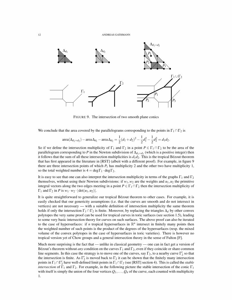
FIGURE 9. The intersection of two smooth plane conics

We conclude that the area covered by the parallelograms corresponding to the points in Γ1∩Γ2 is

area(∆d1+d2)− area∆d1 − area∆d2 =12(d1 +d2)

2− 12

d21 −

12

d22 = d1d2.

So if we define the intersection multiplicity of Γ1 and Γ2 in a point P ∈ Γ1 ∩Γ2 to be the area of theparallelogram corresponding to P in the Newton subdivision of ∆d1+d2 (which is a positive integer) thenit follows that the sum of all these intersection multiplicities is d1d2. This is the tropical Bezout theoremthat has first appeared in the literature in [RST] (albeit with a different proof). For example, in figure 9there are three intersection points of which P1 has multiplicity 2 and the other two have multiplicity 1,so the total weighted number is 4 = degΓ1 ·degΓ2.

It is easy to see that one can also interpret the intersection multiplicity in terms of the graphs Γ1 and Γ2themselves, without using their Newton subdivisions: if w1,w2 are the weights and u1,u2 the primitiveintegral vectors along the two edges meeting in a point P ∈ Γ1∩Γ2 then the intersection multiplicity ofΓ1 and Γ2 in P is w1 ·w2 · |det(u1,u2)|.

It is quite straightforward to generalize our tropical Bezout theorem to other cases. For example, it iseasily checked that our genericity assumptions (i.e. that the curves are smooth and do not intersect invertices) are not necessary — with a suitable definition of intersection multiplicity the same theoremholds if only the intersection Γ1∩Γ2 is finite. Moreover, by replacing the triangles ∆d by other convexpolytopes the very same proof can be used for tropical curves in toric surfaces (see section 1.5), leadingto some very basic intersection theory for curves on such surfaces. The above proof can also be iteratedto the case of hypersurfaces: if n tropical hypersurfaces in Rn intersect in finitely many points thenthe weighted number of such points is the product of the degrees of the hypersurfaces (resp. the mixedvolume of the convex polytopes in the case of hypersurfaces in toric varieties). There is however notropical version yet of Chow groups and a general intersection theory in the sense of Fulton [F].

Much more surprising is the fact that — unlike in classical geometry — one can in fact get a version ofBezout’s theorem without any condition on the curves Γ1 and Γ2, even if they coincide or share commonline segments. In this case the strategy is to move one of the curves, say Γ2, to a nearby curve Γ′2 so thatthe intersection is finite. As Γ′2 is moved back to Γ2 it can be shown that the finitely many intersectionpoints in Γ1∩Γ′2 have well-defined limit points in Γ1∩Γ2 (see [RST] section 4). This is called the stableintersection of Γ1 and Γ2. For example, in the following picture the stable intersection of the conic Γ1with itself is simply the union of the four vertices Q1, . . . ,Q4 of the curve, each counted with multiplicity1.

TROPICAL ALGEBRAIC GEOMETRY 13

Γ1∩Γ2 = {Q1,Q2,Q3,Q4}Γ1∩Γ′2 = {P1,P2,P3,P4}

Γ1 = Γ2Γ′2 Γ1 = Γ2

P3

P2

P1

P4

Q1

Q2

Q4Q3

FIGURE 10. The stable intersection of a conic with itself

The proof of Bezout’s theorem that we have given above is purely combinatorial and does not use thecorresponding classical statement. In fact, we have mentioned already that one of the big advantagesof tropical geometry is that possibly complicated algebraic or geometric questions can be reduced toentirely combinatorial ones. Sometimes it is also interesting and instructive however to remember thattropical geometry is nothing but an “image of classical geometry (over the field K of Puiseux series)under the valuation map”. This way one can try to transfer results from classical geometry directly totropical geometry. In our case at hand we could proceed as follows: if Γ1 and Γ2 are two plane tropicalcurves of degrees d1 and d2 respectively they can be realized as the images under the valuation mapof two classical plane curves C1 and C2 of these degrees over K. Now if we use the classical Bezouttheorem for these curves we can conclude that C1 and C2 intersect in d1d2 points (counted with thecorrect multiplicities). Of course the images of these points under the valuation map are intersectionpoints of Γ1 ∩Γ2, and in a generic situation these will be the only intersection points of these tropicalcurves. To make Bezout’s theorem hold in the tropical setting we therefore should define the intersectionmultiplicity of Γ1 and Γ2 in a point P to be the sum of the intersection multiplicities of C1 and C2 at allpoints that map to P under the valuation map.

Let us check in a simple example that this agrees with the definition of tropical intersection multiplicitythat we have given above. We consider a local situation around an intersection point of Γ1 and Γ2. Forsimplicity let us choose coordinates so that the intersection point is the origin and the two curves havelocal equations Γ1 = {(x1,x2); x2 = 0} and Γ2 = {(x1,x2); x2 = nx1} for some n ∈ N>0. We can thenchoose plane curves C1 and C2 mapping to Γ1 and Γ2 as in the following picture:

1

n

Γ2

x1

x2

Γ2 = {(x1,x2) ∈ R2; x2 = nx1}

C1 = {(z1,z2) ∈ K2; z2 = 1}C2 = {(z1,z2) ∈ K2; z2 = zn

1}

Γ1 = {(x1,x2) ∈ R2; x2 = 0}

Γ1

FIGURE 11. Classical interpretation of the tropical intersection multiplicity

We see that the intersection C1 ∩C2 consists of n points — corresponding to a choice of n-th root ofunity for z1 — that all map to (0,0) in the tropical picture under the valuation map. So the intersectionmultiplicity of Γ1 and Γ2 should be defined to be n. In fact this agrees with our definition above since theprimitive integral vectors of the two tropical curves are u1 = (1,0) and u2(1,n), and |det(u1,u2)|= n.

14 ANDREAS GATHMANN

2.4. The group structure of a plane cubic curve. Again let C be a smooth plane projective complexcurve. The group of divisors DivC on C is the free abelian group generated by the points of C, i.e. thepoints of DivC are finite formal linear combinations D = λ1P1 + · · ·+λnPn with λi ∈ Z and Pi ∈C. Forsuch a divisor we call the number λ1 + · · ·+λn ∈ Z the degree of D. Obviously the subset Div0(C) ofdivisors of degree 0 is a subgroup of DivC.

If C′ is any other curve then the intersection C ∩C′ consists of finitely many points. Hence we canconsider this intersection to be an element of DivC, where we count each point with its intersectionmultiplicity. This divisor is usually denoted C ·C′. By Bezout’s theorem its degree is degC ·degC′.

Two divisors D1,D2 ∈DivC are called equivalent if there are curves C′,C′′ of the same degree such thatD1−D2 =C ·C′−C ·C′′. The group of equivalence classes is usually denoted Pic(C), or Pic0(C) if werestrict to divisors of degree 0.

Now if C has degree 3 it can be shown that after picking a base point P0 ∈C the map C→ Pic0(C),P 7→P−P0 is a bijection. Hence we can use this map to define a group structure on C, or vice versa thestructure of a complex algebraic curve on Pic0(C). Alternatively, it follows by the degree-genus formulathat C has genus 1, i.e. it is a torus. It can be shown that one can realize this torus in the form C/Λ witha lattice Λ ∼= Z2 so that the group structure on C/Λ induced by addition on C is precisely the groupstructure defined by the bijection with Pic0(C) constructed above.

Which of all these results remain true in the tropical world? Let Γ be a plane tropical curve, and letus start by defining the group of divisors DivΓ in the same way as above, i.e. as the free abelian groupgenerated by the points of Γ. As we have seen already that Bezout’s theorem holds in the tropical set-upas well we can also define the group Pic0(Γ) in the same way as before, i.e. it is the group of divisorson Γ of degree 0 modulo those that can be written as Γ ·Γ′−Γ ·Γ′′ for some tropical curves Γ′ and Γ′′

of the same degree.

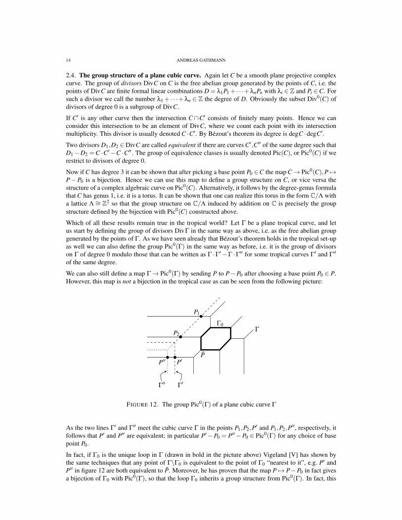
We can also still define a map Γ→ Pic0(Γ) by sending P to P−P0 after choosing a base point P0 ∈ P.However, this map is not a bijection in the tropical case as can be seen from the following picture:

Γ

Γ′Γ′′

P1

P2

P′′ P′P

Γ0

FIGURE 12. The group Pic0(Γ) of a plane cubic curve Γ

As the two lines Γ′ and Γ′′ meet the cubic curve Γ in the points P1,P2,P′ and P1,P2,P′′, respectively, itfollows that P′ and P′′ are equivalent; in particular P′−P0 = P′′−P0 ∈ Pic0(Γ) for any choice of basepoint P0.

In fact, if Γ0 is the unique loop in Γ (drawn in bold in the picture above) Vigeland [V] has shown bythe same techniques that any point of Γ\Γ0 is equivalent to the point of Γ0 “nearest to it”, e.g. P′ andP′′ in figure 12 are both equivalent to P. Moreover, he has proven that the map P 7→ P−P0 in fact givesa bijection of Γ0 with Pic0(Γ), so that the loop Γ0 inherits a group structure from Pic0(Γ). In fact, this

TROPICAL ALGEBRAIC GEOMETRY 15

group structure is just the ordinary group structure of the unit circle S1 after choosing a suitable bijectionof S1 with Γ0.

So to a certain extent we can find analogues of the classical results about plane cubics in the tropicalworld as well. Despite these encouraging results one should note however that there is no good theoryof divisors and their equivalence yet on arbitrary tropical curves.

3. TROPICAL TECHNIQUES IN ENUMERATIVE GEOMETRY

In the last chapter we have seen that many classical results from algebraic geometry have a tropicalcounterpart. However, the main reason why tropical geometry received so much attention recently is thatit can be used very successfully to solve even complicated problems in complex and real enumerativegeometry. So in the rest of this paper we want to give a brief sketch of the progress that has been madeso far in tropical enumerative geometry.

3.1. Complex enumerative geometry and Gromov-Witten invariants. If we stick to plane curves themain basic question in complex enumerative geometry is: given d ≥ 1 and g≥ 0, what are the numbersNg,d of curves of genus g and degree d in the complex projective plane that pass through 3d + g− 1general given points? (The number 3d + g− 1 is chosen so that a naive count of dimensions versusconditions leads one to expect a finite non-zero answer.) Except for some special cases the answer tothis problem has not been known until the invention of Gromov-Witten theory about ten years ago.

For curves in projective spaces the main objects of study in Gromov-Witten theory are the so-calledmoduli spaces of stable maps Mg,n(r,d) for n,r ≥ 0. We will be more specific about the definition ofthese spaces in section 3.2 — for the moment it suffices to say that they are reasonably well-behaved,compact spaces that parametrize curves of genus g and degree d with n marked points in Pr. Of coursethere are evaluation maps evi : Mg,n(r,d)→ Pr for i = 1, . . . ,n that map such an n-pointed curve to theposition of its i-th marked point in Pr.

In the case of plane curves mentioned above we now set n = 3d + g− 1 and choose n general pointsP1, . . . ,Pn ∈P2. The intersection ev−1

1 P1∩·· ·∩ev−1n Pn then obviously corresponds to those plane curves

of the given genus and degree that pass through the specified points. As we have chosen n so that theexpected dimension of this intersection is 0 it makes sense to define the number Ng.d to be the (zero-dimensional) intersection product

ev∗1 P1 · · · · · ev∗n Pn ∈ Z

on Mg,n(r,d). Taking this as a definition has the advantage that we do not have to care about whether(or for which collections of points Pi) the number of curves through the Pi actually is finite — we get awell-defined number in any case. These numbers are called the Gromov-Witten invariants.

In sections 3.2 and 3.3 we will explain how these numbers can actually be computed — both in Gromov-Witten theory and in tropical geometry. For the moment let us just explain how our problem can be setup in the tropical world. In the same way as at the end of section 2.3 the idea is of course simply to mapthe whole situation to the real plane by the logarithm resp. valuation map. A plane curve over C resp.the field of Puiseux series K through some points P1, . . . ,Pn then simply maps to a plane tropical curvein R2 through the n image points. It should therefore also be possible to compute the numbers Ng.d bycounting plane tropical curves of the given genus and degree through n given points in the real plane.The following picture shows the simplest example of this statement, namely that also in the tropicalworld there is always exactly one line through two given (general) points. Note that the relative positionof the points in the plane determines on which edges of the tropical line the points lie (i.e. whether weare in case (a), (b), or (c)):

16 ANDREAS GATHMANN

(a) (b) (c)

FIGURE 13. There is always one tropical line through two given (general) points

This program has been carried out successfully for all Ng,d (and in fact for curves in any toric surface)by Mikhalkin [M1]. One of the main problems when transferring the situation to the tropical world is todetermine — in the same way as for Bezout’s theorem at the end of section 2.3 — how many complexcurves through the given points map to the same tropical curve, i.e. with what multiplicity the tropicalcurves have to be counted. The answer to this question turns out to be surprisingly simple and evenindependent of the chosen points: let Γ⊂ R2 be a tropical curve through the given points. If the pointsare in general position then all vertices of Γ will have valence 3. For any such vertex V we first defineits multiplicity to be w1w2|det(u1,u2)|, where w1,w2,w3 and u1,u2,u3 are the weights and primitiveinteger vectors along the three edges adjacent to V (the balancing condition ensures that it does notmatter which two of the edges we use in the formula). The multiplicity of Γ is then simply the productof the multiplicities of all its vertices. For example, the multiplicity of the following curve is 4 (themultiplicity of both vertices is 2):

(−1,0)2

(0,1)

(2,1)

(−1,−2)

FIGURE 14. A tropical curve whose multiplicity is 4

(Note that this is not a plane curve of some degree since the ends do not point in the right directions forthis. We can interpret figure 14 either as a tropical curve in a different toric surface or as a local pictureof a plane tropical curve.)

Mikhalkin’s “Correspondence Theorem” now states that this is precisely the correct multiplicity for ourpurposes, i.e. that the numbers Ng,d of complex curves through given points P1, . . . ,Pn are the same asthe numbers of tropical curves of the same genus and degree through the images of P1, . . . ,Pn under thelogarithm (resp. valuation) map.

One easy corollary of this statement is worth mentioning: as the numbers of complex curves do notdepend on the choice of points Pi (as long as they are in general position) the same must be true in thetropical setting. To see that this is in fact a non-trivial statement let us consider again the tropical curveof figure 14. Because of the balancing condition this curve is fixed in the plane by the directions of theouter edges and the positions of the three marked points in the plane. If we now move the rightmostpoint down this has the effect of shrinking the bounded edge of the curve (see picture (a) below) untilwe reach a curve with a 4-valent vertex in (b) (note that the slopes of all edges are fixed):

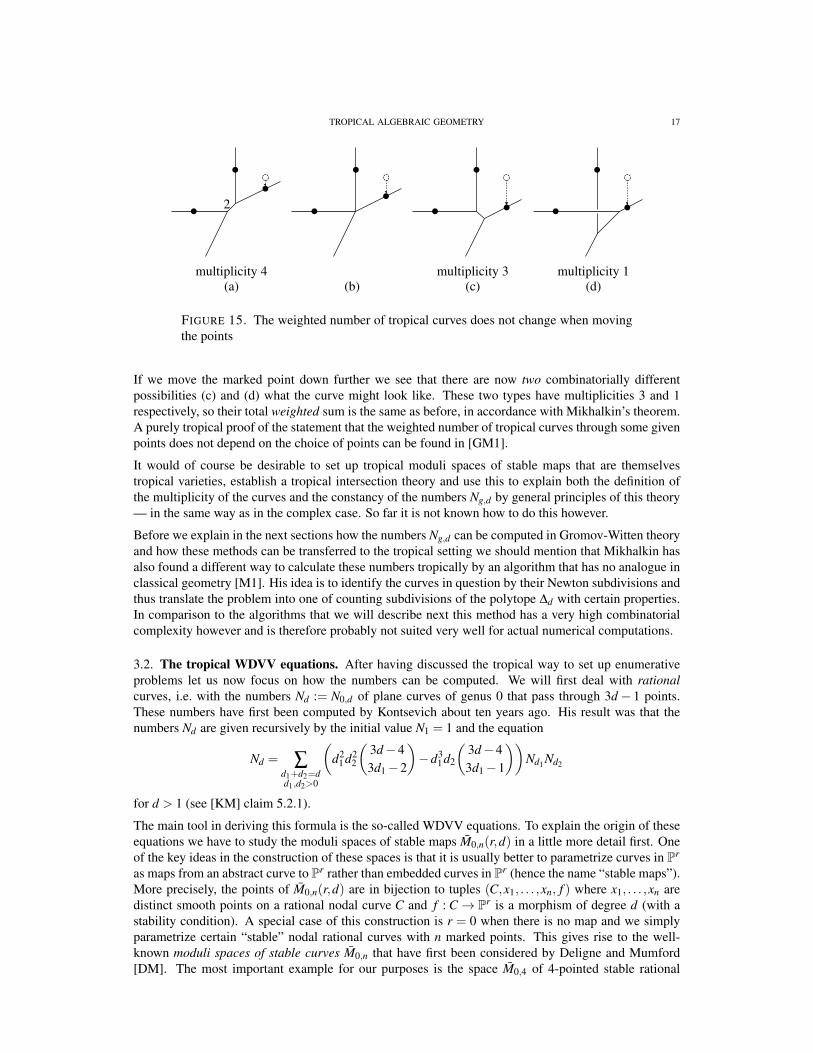
TROPICAL ALGEBRAIC GEOMETRY 17

2

(a) (b)multiplicity 4

(c)multiplicity 3 multiplicity 1

(d)

FIGURE 15. The weighted number of tropical curves does not change when movingthe points

If we move the marked point down further we see that there are now two combinatorially differentpossibilities (c) and (d) what the curve might look like. These two types have multiplicities 3 and 1respectively, so their total weighted sum is the same as before, in accordance with Mikhalkin’s theorem.A purely tropical proof of the statement that the weighted number of tropical curves through some givenpoints does not depend on the choice of points can be found in [GM1].

It would of course be desirable to set up tropical moduli spaces of stable maps that are themselvestropical varieties, establish a tropical intersection theory and use this to explain both the definition ofthe multiplicity of the curves and the constancy of the numbers Ng,d by general principles of this theory— in the same way as in the complex case. So far it is not known how to do this however.

Before we explain in the next sections how the numbers Ng,d can be computed in Gromov-Witten theoryand how these methods can be transferred to the tropical setting we should mention that Mikhalkin hasalso found a different way to calculate these numbers tropically by an algorithm that has no analogue inclassical geometry [M1]. His idea is to identify the curves in question by their Newton subdivisions andthus translate the problem into one of counting subdivisions of the polytope ∆d with certain properties.In comparison to the algorithms that we will describe next this method has a very high combinatorialcomplexity however and is therefore probably not suited very well for actual numerical computations.

3.2. The tropical WDVV equations. After having discussed the tropical way to set up enumerativeproblems let us now focus on how the numbers can be computed. We will first deal with rationalcurves, i.e. with the numbers Nd := N0,d of plane curves of genus 0 that pass through 3d− 1 points.These numbers have first been computed by Kontsevich about ten years ago. His result was that thenumbers Nd are given recursively by the initial value N1 = 1 and the equation

Nd = ∑d1+d2=dd1,d2>0

(d2

1d22

(3d−43d1−2

)−d3

1d2

(3d−43d1−1

))Nd1 Nd2

for d > 1 (see [KM] claim 5.2.1).

The main tool in deriving this formula is the so-called WDVV equations. To explain the origin of theseequations we have to study the moduli spaces of stable maps M0,n(r,d) in a little more detail first. Oneof the key ideas in the construction of these spaces is that it is usually better to parametrize curves in Pr

as maps from an abstract curve to Pr rather than embedded curves in Pr (hence the name “stable maps”).More precisely, the points of M0,n(r,d) are in bijection to tuples (C,x1, . . . ,xn, f ) where x1, . . . ,xn aredistinct smooth points on a rational nodal curve C and f : C→ Pr is a morphism of degree d (with astability condition). A special case of this construction is r = 0 when there is no map and we simplyparametrize certain “stable” nodal rational curves with n marked points. This gives rise to the well-known moduli spaces of stable curves M0,n that have first been considered by Deligne and Mumford[DM]. The most important example for our purposes is the space M0,4 of 4-pointed stable rational

18 ANDREAS GATHMANN

curves. It is well-known that this space is isomorphic to P1. The general point of M0,4 correspondsto a smooth rational curve with 4 distinct marked points, whereas there are also three special pointscorresponding to the curves

x3x4

x2x1 x4x1

x3 x2x1

x2

D12|34 D13|24

x4x3

D14|23

FIGURE 16. The three special points in M0,4

As M0,4 is isomorphic to P1 these three points obviously define the same homology class (resp. the samedivisor) on this moduli space.

The important point is now that there are “forgetful maps” π : M0,n(r,d)→ M0,4 for all n ≥ 4 thatsend a stable map (C,x1, . . . ,xn, f ) to (the stabilization of) (C,x1, . . . ,x4). Pulling back the equalityD12|34 = D13|24 of homology classes on M0,4 we conclude that π∗D12|34 and π∗D13|24 define the samehomology class in M0,n(r,d). Now π∗D12|34 (and similarly of course for π∗D13|24) can be describedexplicitly as the locus of all reducible stable maps with two components such that the marked pointsx1,x2 lie on one component and x3,x4 on the other. Note that this space has many irreducible componentssince the degree and the marked points x5, . . . ,xn can be distributed onto the two components in anarbitrary way.

If we now intersect the equation π∗D12|34 = π∗D13|24 of codimension-1 cycles with suitable cycles ofdimension 1 (that correspond to the condition that the curves in question pass through given subspacesof Pr at the marked points) we get some equations between certain numbers of reducible curves throughgiven points. But these numbers of reducible curves are just products of the corresponding numbers fortheir irreducible components, i.e. products of certain numbers of curves of smaller degree. This way oneobtains recursion formulas that can be shown to determine all the numbers completely (for more detailssee e.g. [CK] section 7.4.2); in the case of P2 we get Kontsevich’s formula stated above.

It has been shown very recently that Kontsevich’s formula can also be proven in essentially the sameway in tropical geometry [GM3]. For a tropical version of the above proof it is very important that wealso adapt the “stable map picture” to the tropical setting, i.e. parametrize plane tropical curves as mapsfrom an “abstract tropical curve” to Pr. Here by abstract tropical curve we simply mean a connectedgraph Γ obtained by glueing closed (not necessarily bounded) real intervals together at their boundarypoints in such a way that every vertex has valence at least 3. In particular, every bounded edge of suchan abstract tropical curve has an intrinsic length. Following an idea of Mikhalkin [M3] the unboundedends of Γ will be labeled and called the marked points of the curve. The most important example for ourapplications is of course the “tropical M0,4” whose points correspond to tree graphs with 4 unboundedends. There are four possible combinatorial types for this:

x3x1

x2

x1 x1

x2

x1

x4 x4

x3

x4x3

x2

x4

x2

x3

l l l

(a) (b) (c) (d)

FIGURE 17. The four combinatorial types of curves in the tropical M0,4

In the types (a) to (c) the bounded edge has an intrinsic length l; so each of these types leads to a stratumof M0,4 isomorphic to R>0 parametrized by this length. The last type (d) is simply a point in M0,4 that

TROPICAL ALGEBRAIC GEOMETRY 19

can be seen as the boundary point where the other three strata meet. Hence M0,4 is again a rationaltropical curve:

(a)

(c)

(d)

(b)

M0,4

FIGURE 18. M0,4 is again a rational tropical curve

In analogy to the complex case plane tropical curves are now parametrized as tuples (Γ,x1, . . . ,xn,h),where Γ is an abstract tropical curve, x1, . . . ,xn are distinct unbounded ends of Γ, and h : Γ→ R2 is apiecewise linear map with certain conditions (see [GM3] for details). The most important feature of thisdefinition is that h may be a constant map on some edges of Γ, and is in fact required to be a constantmap on the unbounded ends x1, . . . ,xn. For example, the following picture shows a 4-pointed planetropical conic, i.e. of the tropical analogue of M0,4(2,2):

x1

x2x3 x4

h

R2Γh(x1)

h(x2)h(x3)

h(x4)

l

FIGURE 19. A tropical stable map in M0,4(2,2)

Note that the balancing condition around every (3-valent) vertex adjacent to a marked point (resp. edge)xi ensures that the other two edges around this vertex form a straight line in R2.

It is easy to see from this picture already that the tropical moduli spaces M0,n(r,d) with n ≥ 4 admitforgetful maps to M0,4: given an n-marked plane tropical curve (Γ,x1, . . . ,xn,h) we simply forget themap h, take the minimal connected subgraph of Γ that contains x1, . . . ,x4, and “straighten” this graphto obtain an element of M0,4. In the picture above we simply obtain the “straightened version” of thesubgraph drawn in bold, i.e. the element of M0,4 of type (a) in figure 17 with length parameter l asindicated in the picture.

To obtain the WDVV equations we now simply consider the inverse image under this forgetful map of apoint of M0,4 of type (a) resp. (b) in figure 17 with a very large length parameter l. It can be shown thatsuch very large lengths can occur only if there is a bounded edge (of a very large length) in Γ on whichh is constant:

20 ANDREAS GATHMANN

h

R2Γx1

x2

h(x1)

h(x2)

h(x4)h(x3)

x3

x4

E

l

h(E)

FIGURE 20. A very large length in M0,4 leads to a tropical stable map with a con-tracted bounded edge

Again the balancing condition around the contracted bounded edge requires that the image of the tropicalcurve in R2 is locally a union of two straight lines. We can therefore consider such curves as beingreducible and made up of two tropical curves of smaller degrees (in figure 20 we have a reducibletropical conic that is a union of two tropical lines). The picture is now exactly the same as in theclassical case, and in fact the rest of the proof of Kontsevich’s formula works in the same way as inGromov-Witten theory. It is expected that essentially the same proof can be used to reprove the WDVVequations for rational curves in higher-dimensional spaces as well.

This application of tropical geometry shows very well that it should be possible to carry many conceptsfrom classical complex geometry over to the tropical world: moduli spaces of curves and stable maps,morphisms, divisors and divisor classes, intersection multiplicities, and so on. In [GM3] these conceptswere introduced only in the specific cases needed for Kontsevich’s formula.

3.3. The tropical Caporaso-Harris formula. After having discussed rational curves let us now turnto the general numbers Ng,d for arbitrary genus g. These numbers have first been computed by Caporasoand Harris [CH]. The idea in their proof is is to define new invariants that count plane curves of givendegree and genus having specified local contact orders to a fixed line L and passing in addition throughthe appropriate number of general points. By specializing one point after the other to lie on L one canthen derive recursive relations among these new invariants that finally suffice to compute all the numbersNg,d .

Instead of explaining the general formula let us look at an example of what happens in this specializationprocess, referring to [CH] for details. We consider plane rational cubics having a point of contact order3 to L at a fixed point P1 ∈ L and passing in addition through 5 general points P2, . . . ,P6 ∈ P2 as in thefollowing picture on the left:

L

specializeP6 P5P1 P2 P3 P4

L L

+P1P2

P1

P2

FIGURE 21. Computing the number of cubics with a point of contact order 3 to a line

To compute the number of such curves we specialize P2 to lie on L. As the cubics intersect L alreadywith multiplicity 3 at P1 they cannot pass through another point on L unless they become reducibleand have L as a component. Hence there are two possibilities after the specialization (see figure 21):the cubics can degenerate into a union of three lines L∪ L1 ∪ L2 where L1 and L2 each pass through

TROPICAL ALGEBRAIC GEOMETRY 21

two of the points P3, . . . ,P6, or they can degenerate into L∪C, where C is a conic tangent to L andpassing through P3, . . . ,P6. The initial number of rational cubics with a point of contact order 3 to L at afixed point and passing through 5 more general points is therefore a sum of two numbers (counted withsuitable multiplicities) related to only lines and conics. This is the general idea of Caporaso and Harrishow specialization finally reduces the degree of the curves and allows a recursive solution to computethe numbers Ng,d as well as all the newly introduced numbers of curves with multiplicity conditions.

In fact, the same constructions can again be made in tropical geometry [GM2]. Intuitively, if we pickour line L⊂C2 to be the line with z1-coordinate 0 then its image under the logarithm map is “the verticalline with x1-coordinate −∞”. Hence the process of moving P2 to the line L in complex geometry nowsimply corresponds to moving P2 to the very far left in tropical geometry. Moreover, curves with highercontact orders to L in complex geometry just correspond to tropical curves with unbounded ends ofhigher weight to the left. So the tropical analogue of the specialization process of figure 21 is

P3

3 + 33 2P1

P2P4 P6

P5

P1

P2

P1

P2

FIGURE 22. The degeneration of figure 21 in the tropical setting

where P1 is to be considered to lie infinitely far to the left. Note that the curves after moving P2 to theleft are not reducible, but they still “split” into two parts: a left part (through P2) and a right part (throughthe remaining points, circled in the picture above). We get the same “degenerations” as in the complexcase: one where the right part consists of two lines through two of the points P3, . . . ,P6 each, and onewhere it consists of a conic “tangent to a line” (i.e. with an unbounded edge of multiplicity 2 to the left).

Using this idea it has been shown in [GM2] that the Caporaso-Harris formula can also be proven intropical geometry — in fact with a much simpler proof than in complex geometry since we are onlydealing with combinatorial objects and do not have to construct and study complicated moduli spacesin complex geometry.

3.4. Real enumerative geometry and Welschinger invariants. Of course, the same questions as inthe previous sections can be asked for real instead of for complex curves: given d ≥ 1, g ≥ 0, and3d + g− 1 points in general position in the real projective plane P2

R, how many curves of degree dand genus g are there in P2

R that intersect all the given points? Note that every such real curve hasa complexification by just considering its equation as an equation in the complex rather than the realplane, and by its degree and genus we simply mean the degree resp. genus of its complexification.

As usual in algebraic geometry this real case is much more difficult to handle than the complex case.The first problem is already that the answer to this question will in general depend on the position ofthe points so that there are no well-defined numbers Ng,d as in the complex case. Instead one could askquestions of the following type:

• is there at least one real curve of degree d and genus g through any choice of 3d +g−1 givenpoints? Or even better: can we compute a lower bound for the number of real curves throughany choice of points?

• Is there a way to assign multiplicities to the real curves through the given points so that theweighted sum of these curves is independent of the choice of points?

A few years ago Welschinger has found a solution to the second question for the case of curves of genus0 [W]. To state his result note first that a general complex plane rational curve of degree d has exactly

22 ANDREAS GATHMANN

12 (d−1)(d−2) nodes, i.e. points where two smooth branches of the curve intersect transversally. If C isnow a real rational plane curve then each of the nodes of its complexification is of one of the followingthree types:

(a) nodes that are in the real plane P2R and where the local equation of the curve is of the form

x2− y2 = 0, i.e. (x+ y)(x− y) = 0 for suitable local analytic coordinates. In a local real pictureC is simply the union of two smooth curves intersecting transversely.

(b) nodes that are in the real plane P2R and where the local equation of the curve is of the form

x2 +y2 = 0 for suitable local analytic coordinates. In a local real picture such a node leads to anisolated point corresponding to the values x = y = 0.

(c) nodes that are not in the real plane P2R. These nodes obviously come in pairs as the complex

conjugate of such a node is again a node of the complexification. They are not visible in the realcurve C.

Welschinger’s main theorem is now the following: if we assign to each real plane curve C the multiplic-ity (−1)m where m is the number of nodes of type (b) of its complexification then the correspondingweighted sum of all curves through the given points is independent of the choice of points. It is calledthe Welschinger invariant Wd . In particular, Wd gives a lower bound for the actual number of real planecurves through any set of 3d−1 general given points, whereas the complex number N0,d is of course anupper bound.

Unfortunately, except for a few special cases Welschinger was not able to actually compute the numbersWd . So the question whether there always exists a real rational plane curve of degree d through any setof 3d−1 general points remained open.

Some time ago however a tropical way has been found to compute the Welschinger invariants Wd andin fact also the actual (non-invariant) numbers of real curves through some configurations of points inthe plane [IKS1, M1]. In the same way as in Mikhalkin’s Correspondence Theorem the strategy is toidentify complex resp. real algebraic curves with tropical curves, and then to count such tropical curveswith the proper multiplicities. More precisely, to obtain the Welschinger invariant Wd one has to countrational plane tropical curves of degree d through 3d−1 points in the same way as for the computationof N0,d — but one does not count them with the “complex multiplicity” as described in section 3.1, butrather with the multiplicity

0 if the “complex multiplicity” is even,1 if the “complex multiplicity” is congruent to 1 modulo 4,−1 if the “complex multiplicity” is congruent to 3 modulo 4.

One can then try to do this count by enumerating the corresponding Newton subdivisions of the poly-tope ∆d as in section 1.4. Although the algorithm is combinatorially very complicated (and cannot beexplained here in detail) it can be used to prove that the numbers Wd are all positive and hence that thereis always at least one real rational plane curve of degree d through any set of 3d− 1 points in generalposition. In fact, a more careful study of the algorithm even allows one to prove that the lower andupper bounds Wd resp. N0,d for the numbers of these curves grow approximately with the same speed asd increases [IKS2].

Very recently Itenberg has shown that both the proof of [GM1] that the invariants are independent of themarked points and the proof of [GM2] of the tropical Caporaso-Harris formula (see section 3.3) can beadapted to the Welschinger case. In particular, this yields a “real Caporaso-Harris formula” that gives afast method to compute the Welschinger invariants. It is not known yet whether there exists an analogueof the WDVV equations (see section 3.2) in the real case.

TROPICAL ALGEBRAIC GEOMETRY 23

CONCLUSION

In the last few years tropical algebraic geometry has evolved with a tremendous speed. Its generalapproach to replace algebro-geometric problems by combinatorial ones often leads to new insights,sometimes to easier proofs of known statements, and occasionally even to new results in algebraicgeometry.

Nevertheless tropical geometry is still in its beginnings since even the most basic objects of algebraicgeometry — (abstract) varieties and their morphisms — do not have a satisfactory counterpart yet in thetropical world. Consequently, there are many open problems in tropical geometry for the near future, andone could reasonably expect that the solution to these problems gives an entirely new strategy to attackmany problems in algebraic geometry. In fact, two such recent new examples in which tropical ideashave already been applied successfully are the study of compactifications of subvarieties of algebraictori (in particular moduli spaces of rational stable curves) [Te] and low-dimensional topology [Ti].

REFERENCES

[BJSST] T. Bogart, A. Jensen, D. Speyer, B. Sturmfels, R. Thomas, Computing tropical varieties, preprint math.AG/0507563.[CH] L. Caporaso, J. Harris, Counting plane curves of any genus, Invent. Math. 131 (1998), 345–392.[CK] D. Cox, S. Katz, Mirror symmetry and algebraic geometry, Mathematical Surveys and Monographs 68, AMS.[DM] P. Deligne, D. Mumford: The irreducibility of the space of curves of given genus. IHES 36 (1969), 75–110.[F] W. Fulton, Intersection theory, Ergebnisse der Mathematik und ihrer Grenzgebiete, Springer (1984).[GL] S. Gao, A. Lauder, Decomposition of polytopes and polynomials, Discrete and Computational Geometry 26 (2004),

89–104.[GM1] A. Gathmann, H. Markwig, The number of tropical plane curves through points in general position, preprint math.AG/

0504390.[GM2] A. Gathmann, H. Markwig, The Caporaso-Harris formula and plane relative Gromov-Witten invariants in tropical

geometry, preprint math.AG/0504392.[GM3] A. Gathmann, H. Markwig, Kontsevich’s formula and the WDVV equations in tropical geometry, preprint math.AG/

0509628.[IKS1] I. Itenberg, V. Kharlamov, and E. Shustin, Welschinger invariant and enumeration of real rational curves, Int. Math.

Res. Not. 2003 no. 49 (2003), 2639–2653.[IKS2] I. Itenberg, V. Kharlamov, and E. Shustin, Logarithmic equivalence of the Welschinger and the Gromov-Witten invari-

ants, Russ. Math. Surv. 59 no. 6 (2004), 1093–1116.[IMTI] H. Imai, T. Masada, F. Takeuchi, K. Imai, Enumerating triangulations in general dimensions, Int. J. Comput. Geom.

Appl. 12 no. 6 (2002), 455–480.[J] A. Jensen, Gfan — a software system for Grobner fans, http://home.imf.au.dk/ajensen/software/gfan/gfan.html (2005).[K] M. Kapranov, Amoebas over non-archimedean fields, preprint (2000).[KM] M. Kontsevich, Y. Manin, Gromov-Witten classes, quantum cohomology, and enumerative geometry, Commun. Math.

Phys. 164 (1994), 525–562.[M1] G. Mikhalkin, Enumerative tropical algebraic geometry in R2, J. Amer. Math. Soc. 18 (2005), preprint math.AG/

0312530.[M2] G. Mikhalkin, Tropical geometry, preprint (2005).[M3] G. Mikhalkin, Tropical curves and their Jacobians, preprint (2005).[R] J. Rambau, TOPCOM: Triangulations of point configurations and oriented matroids, in: Mathematical software –

ICMS 2002 (A. Cohen, X. Gao, N. Takayama, eds.), World Scientific (2002), 330–340.[RST] J. Richter-Gebert, B. Sturmfels, T. Theobald, First steps in tropical geometry, in: Idempotent Mathematics and Math-

ematical Physics (G. Litvinov, V. Maslov, eds.), Proceedings Vienna 2003, American Mathematical Society, Contemp.Math. 377 (2005), 289–317.

[Si] I. Simon, Recognizable sets with multiplicities in the tropical semiring, Mathematical foundations of computer science(Carlsbad 1988), Springer Lecture Notes in Computer Science 324 (1988), 107–120.

[Sh] E. Shustin, Patchworking singular algebraic curves, non-archimedean amoebas, and enumerative geometry, preprintmath.AG/0211278.

[Sp] D. Speyer, Tropical geometry, PhD thesis, UC Berkeley (2005).[SS] D. Speyer, B. Sturmfels, Tropical mathematics, preprint math.CO/0408099.[Te] J. Tevelev, Compactifications of subvarieties of tori, preprint math.AG/0412329.[Th] T. Theobald, On the frontiers of polynomial computations in tropical geometry, preprint math.CO/0411012.[Ti] S. Tillmann, Boundary slopes and the logarithmic limit set, preprint math.GT/0306055.[V] M. Vigeland, The group law on a tropical elliptic curve, preprint math.AG/0411485.

24 ANDREAS GATHMANN

[W] J. Welschinger, Invariants of real rational symplectic 4-manifolds and lower bounds in real enumerative geometry, C.R. Math. Acad. Sci. Paris 336 no. 4 (2003), 341–344.

ANDREAS GATHMANN, FACHBEREICH MATHEMATIK, TECHNISCHE UNIVERSITAT KAISERSLAUTERN, POSTFACH 3049,67653 KAISERSLAUTERN, GERMANY

E-mail address: andreas@mathematik.uni-kl.de