KNOCK PREDICTION INGAS-FIREDRECIPROCATING ENGINESDevelopment of a zero-dimensional two zone model including detailed chemical kinetics

A. Trijselaar

FACULTY OF ENGINEERING TECHNOLOGYFACULTY OF ENGINEERING TECHNOLOGYDEPARTMENT OF THERMAL ENGINEERING

EXAMINATION COMMITTEEprof. dr. ir. M. Woltersdr. ir. J.B.W. Kokdr. ir. A.G.J. van der Hamir. H. de Laat

Enschede, January 2012Enschede, January 2012

1

Summary

The composition of natural gas supplied in the Netherlands is changing as a result of increasing imports and

developments in the field of sustainable gas sources. One of the risks associated with this transition to other

types of gas is the occurrence of knock in gas-fired reciprocating engines. Engine knock is the phenomenon

where part of the unburnt air-fuel mixture in the cylinder autoignites before it is consumed by the flame

front originating from the spark plug. The heavy pressure oscillations resulting from autoignition can cause

considerable damage to the engine. In this respect more information is required on the knock tendency of

possible future gas qualities.

Experimental knock research is both expensive and time consuming. Internal combustion engine modeling

offers an inexpensive and fast alternative for experiments. The goal of the research is therefore to develop an

engine model capable of predicting whether knock will occur when a particular engine is running on a

gaseous fuel of specified composition.

Based on a literature study and progress of research partners in this field a zero-dimensional two zone

model including detailed chemical kinetics has been developed. Based on basic engine parameters and gas

composition the compression and combustion phase of an Otto cycle has been simulated. Output consists of

knock intensity, in-cylinder temperature and pressure, heat release and species concentrations. The model

has been validated by experiments performed on a gas-fired reciprocating engine of a combined heat and

power (CHP) unit fueled by blends of natural gas, hydrogen and carbon monoxide.

The model is able to accurately simulate the in-cylinder pressure for natural gas operation in the span of

spark advance measured during the experiments. For blends of natural gas and hydrogen the pressure

curves show more deviation from the experiments, especially at low fractions of hydrogen. This is caused by

an overprediction of the laminar flame speed by the numerical code used. When the laminar flame speed is

corrected for the lower flammability limit of hydrogen the simulations show good agreement with the

experiments with natural gas-hydrogen blends. More important, the knock intensity predicted by the model

can be directly related to the knock intensity measured during the experiments. The results agree for all gas

compositions used in the experiments, indicating that the model is indeed capable of predicting the

occurrence of knock for at least blends of natural gas and hydrogen. Results also indicate that the model

might be able to accurately predict knock occurrence in blends of natural gas and propane, while the model

is expected to be inaccurate for blends of natural gas and ethane. This has however not been validated by

experiments.

This research shows it is possible to accurately predict knock occurrence using a zero-dimensional two zone

model including detailed chemical kinetics. The accuracy of the predictions however strongly depends on

the suitability of the chemical mechanism used. The mechanisms nC5_50 and C3_41 used in this research are

capable of accurately simulating the knocking behavior of blends of natural gas and hydrogen and possibly

of blends of methane and propane as well. The frequently used mechanism GRI Mech 3.0 is unsuitable for

knock prediction. All three mechanisms are suitable for prediction of in-cylinder pressure.

Future work should focus on improving the laminar flame speed prediction, determining a critical value of

the knock criterion and experimental validation of the simulations of blends of natural gas and higher

hydrocarbons. The validity of the model for turbocharged and lean burn engines might be validated as well.

2

Acknowledgements

This Master‟s thesis marks the end of nine months of research and the end of a splendid period of studying

Mechanical Engineering at the University of Twente. My interest in the subject of changing gas composition

in the Dutch gas grid was raised during the course Gas Technology by professor Wolters. After completing

the course with a report on this subject the idea of writing my Master‟s thesis on the same subject arose. I am

therefore very thankful that I have been given the opportunity by Kiwa Gas Technology to participate in

more in-depth research in this field.

I would like to thank Hans de Laat for guiding this research on behalf of Kiwa Gas Technology and Mannes

Wolters for supervising on behalf of the University of Twente. I really appreciate the help given by the

following people from Kiwa Gas Technology: Mathijs Kippers, Wim Bouwman and Mindert van Rij. Finally,

I would like to express my gratitude towards Jim Kok and Louis van der Ham from the University of

Twente for being available for help and for assessing my Master‟s assignment. The funding for this project

by Gasterra was warmly appreciated.

I hope the results of this research will contribute to the work of Kiwa Gas Technology and will be input for a

lively discussion during the defense of my thesis.

Enschede, January 2012

3

Contents

Summary ......................................................................................................................................................................... 1

Acknowledgements ...................................................................................................................................................... 2

Contents .......................................................................................................................................................................... 3

1 Introduction ........................................................................................................................................................... 5

2 Literature study ..................................................................................................................................................... 7

2.1 Knock phenomenon ........................................................................................................................................ 7

2.1.1 Factors influencing knock occurrence ................................................................................................. 9

2.2 Knock modeling ............................................................................................................................................. 10

2.2.1 Geometry models ................................................................................................................................. 11

2.2.2 Knock models ....................................................................................................................................... 12

2.2.3 Engine correlations .............................................................................................................................. 13

2.3 Experimental knock research ....................................................................................................................... 15

2.3.1 Knock detection .................................................................................................................................... 15

2.3.2 Fuel knock resistance classification ................................................................................................... 16

2.4 Chemical kinetics ........................................................................................................................................... 16

2.5 Final considerations ...................................................................................................................................... 18

3 Research method ................................................................................................................................................. 19

3.1 Model description .......................................................................................................................................... 19

3.1.1 General description.............................................................................................................................. 19

3.1.2 Fundamental equations ....................................................................................................................... 20

3.1.3 Software implementation .................................................................................................................... 23

3.2 Experimental setup and procedure ............................................................................................................. 23

3.2.1 Engine .................................................................................................................................................... 23

3.2.2 Data acquisition system ...................................................................................................................... 23

3.2.3 Gas compositions ................................................................................................................................. 24

3.2.4 Experimental procedure...................................................................................................................... 24

4 Results ................................................................................................................................................................... 26

4.1 Knock prediction model ............................................................................................................................... 26

4.1.1 User input ............................................................................................................................................. 26

4.1.2 Compression stroke ............................................................................................................................. 28

4.1.3 Combustion phase ............................................................................................................................... 30

4.2 Experimental validation ............................................................................................................................... 33

4.2.1 Spark timing ......................................................................................................................................... 33

4.2.2 Gas composition ................................................................................................................................... 35

4.2.3 Knock criterion and knock limit spark time ..................................................................................... 39

4.2.4 Cylinder-to-cylinder variations .......................................................................................................... 41

4

4.2.5 Blow-by measurement ........................................................................................................................ 43

4.3 Correspondence with methane number ..................................................................................................... 44

4.4 Model developments ..................................................................................................................................... 47

4.4.1 Turbulence factor ................................................................................................................................. 47

4.4.2 Ignition lag ............................................................................................................................................ 48

4.5 Sensitivity analysis ........................................................................................................................................ 49

4.5.1 Engine parameters ............................................................................................................................... 49

4.5.2 Other model parameters ..................................................................................................................... 50

4.5.3 Time step ............................................................................................................................................... 51

5 Conclusions and recommendations ................................................................................................................. 52

5.1 Conclusions .................................................................................................................................................... 52

5.2 Recommendations ......................................................................................................................................... 52

References .................................................................................................................................................................... 53

Nomenclature .............................................................................................................................................................. 55

5

1 Introduction

Background

After the discovery of the Slochteren natural gas field in 1959 the Dutch government rapidly started

developing a nationwide gas grid, making it possible to supply nearly every household with „Groningen

quality‟ natural gas. As opposed to most other major gas fields in the world the Slochteren field contains low

calorific natural gas (L-gas), which indicates the heating value of the gas is relatively low. This difference is

caused by a relatively high fraction of inert nitrogen gas and a relatively low fraction of higher

hydrocarbons (ethane and up) in Slochteren natural gas. As a result all domestic (i.e. households and

businesses) gas appliances in the Netherlands are designed to operate using low calorific natural gas.

Liberalization of the Dutch gas market and the ongoing reduction of the Dutch natural gas reserves have

caused a considerable rise in natural gas imports over the last 15 years. Currently the largest part of these

imports originates from Norway and Russia, which both supply high calorific natural gas (H-gas).

Furthermore, the imports of liquid natural gas (LNG) are expected to increase significantly over the

upcoming years. LNG also tends to be high calorific, because the required cleaning process results in a

relatively high purity. These H-gases cannot be fed directly into the Dutch gas grid, because it could cause

flame instability or incomplete combustion in appliances intended for burning L-gas. Currently these

imported gases are blended with inert nitrogen gas up to a level where they comply with Dutch standards.

Another development resulting in a varying gas composition in the Dutch gas grid is the increasing use of

sustainable energy sources. Gasification of biomass results in synthesis gas: a mixture of hydrogen gas and

carbon monoxide. Another option is digestion of biomass, which results in a mixture of methane and carbon

dioxide. Finally, creating hydrogen gas using fuel cells is considered a viable option for storing excessive

electricity generated by for example wind turbines and solar panels. Synthesis gas, biogas and pure

hydrogen gas can all be blended with natural gas to account for a sustainable part of the Dutch gas supply,

but since neither hydrogen nor carbon monoxide are components of natural gas the influence on end-use

equipment should be investigated.

Problem statement

One of the concerns of varying gas composition in the Dutch gas grid is the occurrence of knock in gas-fired

reciprocating engines: heavy pressure oscillations in the cylinders which can cause considerable damage to

the engine. Most engines run safely over the whole range of operating conditions when firing natural gas.

Since some gaseous fuels like hydrogen and higher hydrocarbons are more prone to knocking than

methane, future gas compositions could cause engines to show knocking combustion when firing gas from

the grid. The main problem in predicting whether knock will occur is that this depends on a large number of

parameters, related not only to gas composition, but to engine geometry and engine operating conditions as

well.

Research goal

Experimental research is time consuming and expensive, hence not very suitable for investigating a large

number of engines and gas compositions. Furthermore, there is a risk of damaging the test engine when

performing experimental knock research. Engine simulation can offer a suitable alternative for experimental

research, making it possible to investigate various gas compositions, engine geometries and operating

conditions in a relatively short amount of time. The goal of this research is therefore the development of a

modeling tool capable of predicting knock occurrence based on gas composition and engine parameters.

Research approach

A literature study has been carried out to get acquainted with different aspects of the subject. Based on the

literature study a zero-dimensional two zone model has been developed, capable of predicting engine knock

using gas composition and engine data as input. The model has been validated by experiments performed

on a combined heat and power (CHP) engine at the Kiwa Gas Technology laboratory.

Introduction 6

Structure of the report

The report starts with an overview of the literature study in chapter 2. Consecutively the physical

characteristics of knock, existing methods of knock modeling, experimental knock research and fundamental

chemical kinetics of knock are treated here. Chapter 3 describes the research method, starting with the

method used for modeling, followed by a description of the experimental setup and experimental

procedure. The results of the research are treated in chapter 4, which starts with an extensive description of

the developed model. Next, results of the experiments and simulations are presented for validation and

sensitivity analysis of the model. Finally, chapter 5 contains the conclusions of the research, as well as

recommendations for future work.

Knock phenomenon 7

2 Literature study

To fully understand the subject of engine knock and get acquainted with the current state of research in the

field, a literature study has been performed. This chapter starts with a general discussion of knock, treating

the physical processes which define the phenomenon, possible causes and different types of engine knock.

The next paragraph gives an overview of the current state of knock modeling, focusing on possibilities for

engine geometry modeling, knock prediction and three correlations useful for modeling internal combustion

engines. To prepare for the experimental part of the research the third paragraph gives an overview of

experimental knock research, treating the way knock is determined experimentally and the way fuels are

classified based on knock resistance. The final paragraph gives a more in-depth view on the chemical

kinetics behind engine knock, which is useful for a more fundamental understanding of the problem as well

as for determining which types of modeling are suitable for engine knock.

2.1 Knock phenomenon

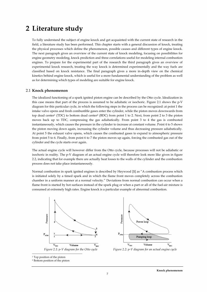
The idealized functioning of a spark ignited piston engine can be described by the Otto cycle. Idealization in

this case means that part of the process is assumed to be adiabatic or isochoric. Figure 2.1 shows the p-V

diagram for this particular cycle, in which the following steps in the process can be recognized: at point 1 the

intake valve opens and fresh combustible gases enter the cylinder, while the piston moves downwards from

top dead center1 (TDC) to bottom dead center2 (BDC) from point 1 to 2. Next, from point 2 to 3 the piston

moves back up to TDC, compressing the gas adiabatically. From point 3 to 4 the gas is combusted

instantaneously, which causes the pressure in the cylinder to increase at constant volume. Point 4 to 5 shows

the piston moving down again, increasing the cylinder volume and thus decreasing pressure adiabatically.

At point 5 the exhaust valve opens, which causes the combusted gases to expand to atmospheric pressure

from point 5 to 6. Finally, from point 6 to 7 the piston moves up again, forcing the combusted gas out of the

cylinder and the cycle starts over again.

The actual engine cycle will however differ from the Otto cycle, because processes will not be adiabatic or

isochoric in reality. The p-V diagram of an actual engine cycle will therefore look more like given in figure

2.2, indicating that for example there are actually heat losses to the walls of the cylinder and the combustion

process does not take place instantaneously.

Normal combustion in spark ignited engines is described by Heywood [1] as “A combustion process which

is initiated solely by a timed spark and in which the flame front moves completely across the combustion

chamber in a uniform manner at a normal velocity.” Deviations from normal combustion can occur when a

flame front is started by hot surfaces instead of the spark plug or when a part or all of the fuel-air mixture is

consumed at extremely high rates. Engine knock is a particular example of abnormal combustion.

Figure 2.1: p-V diagram for the Otto cycle Figure 2.2: p-V diagram for an actual engine cycle

1 Top position of the piston 2 Bottom position of the piston

Literature study 8

According to Heywood knock refers to the phenomenon when spontaneous ignition of the end-gas (the part

of the gas which has not yet been consumed by the flame) causes an extremely rapid release of the chemical

energy in the end-gas. As a result very high local pressures occur in the cylinder and pressure waves

propagate through the combustion chamber. These pressure waves can cause the combustion chamber to

resonate at its natural frequency, resulting in the audible noise known as knock. An example of the high

frequency pressure fluctuations occurring in the cylinder during knock can be found in the pressure

diagrams of figure 2.3. The leftmost graph gives a typical course of pressure during normal combustion. The

center graph shows the occurrence of light knock late in the burning process. The rightmost graph is a

typical example of heavy knock, occurring earlier in the process and thus closer to top dead center. It is

important to note that once knocking occurs the pressure distribution over the cylinder is no longer uniform

and the measured cylinder pressure therefore depends on the location of the sensor.

Although there is no complete fundamental explanation of the knock phenomenon yet, there are two

generally accepted theories on the rapid release of chemical energy which causes knock [1]. The autoignition

theory assumes the end-gas region is compressed to such high pressures and temperatures that spontaneous

combustion of the remaining fuel-air mixture occurs. The detonation theory on the other hand is based on

acceleration of the flame front to sonic velocity, which consumes the end-gas at a much faster rate than

would be the case during normal combustion. According to Heywood [1], most recent evidence however

indicates an extremely rapid sequence of reactions in the end-gas initiated by autoignition of local regions as

the origin of knock. The autoignition theory has thus become the most widely accepted explanation for

knock. The chemical mechanisms behind these autoignition processes are treated in paragraph 2.4.

After autoignition the sharp rise in temperature and pressure of the end-gas region results in a shockwave

which travels into the burnt gas region. Reflection of these waves on the walls of the cylinder eventually

results in standing waves of which the amplitude increases at first, and damps out eventually. These are the

characteristic pressure oscillations shown in figure 2.3.

The danger of knock occurrence is that it can cause severe damage to engines. Due to the additional heat

load under knocking conditions, the cylinder head and piston tend to overheat which can cause even more

intense knocking. When not stopped in time the engine will overheat and the piston and piston rings can

contact the cylinder wall, which causes serious damage at regular engine speeds. Furthermore the higher

heat loads will weaken the engine materials and in combination with the locally elevated pressures pitting,

erosion and breakage of cylinder and piston parts can occur within a small time span.

Another -but for this research less relevant- type of abnormal combustion is surface ignition, in which

ignition is triggered by a hot surface instead of the ignition spark. Well known examples of hot surfaces are

overheated exhaust valves and glowing carbon deposits in the combustion chamber. Depending on whether

this happens before or after the spark the phenomenon is called preignition or postignition respectively.

Since this effect is triggered by for example an overheated spark plug or glowing deposit, it is very hard to

predict and shall therefore not be treated extensively. It is however important to mention, because surface

ignition usually results in a sharp rise in temperature and pressure and is therefore likely to cause knock. In

this case the phenomenon is called knocking surface ignition, as opposed to spark knock which can occur

during normal combustion.

Figure 2.3: Typical pressure-crank angle diagrams for normal combustion (left), slight knocking combustion (center)

and heavy knocking combustion (right) [1]

Knock phenomenon 9

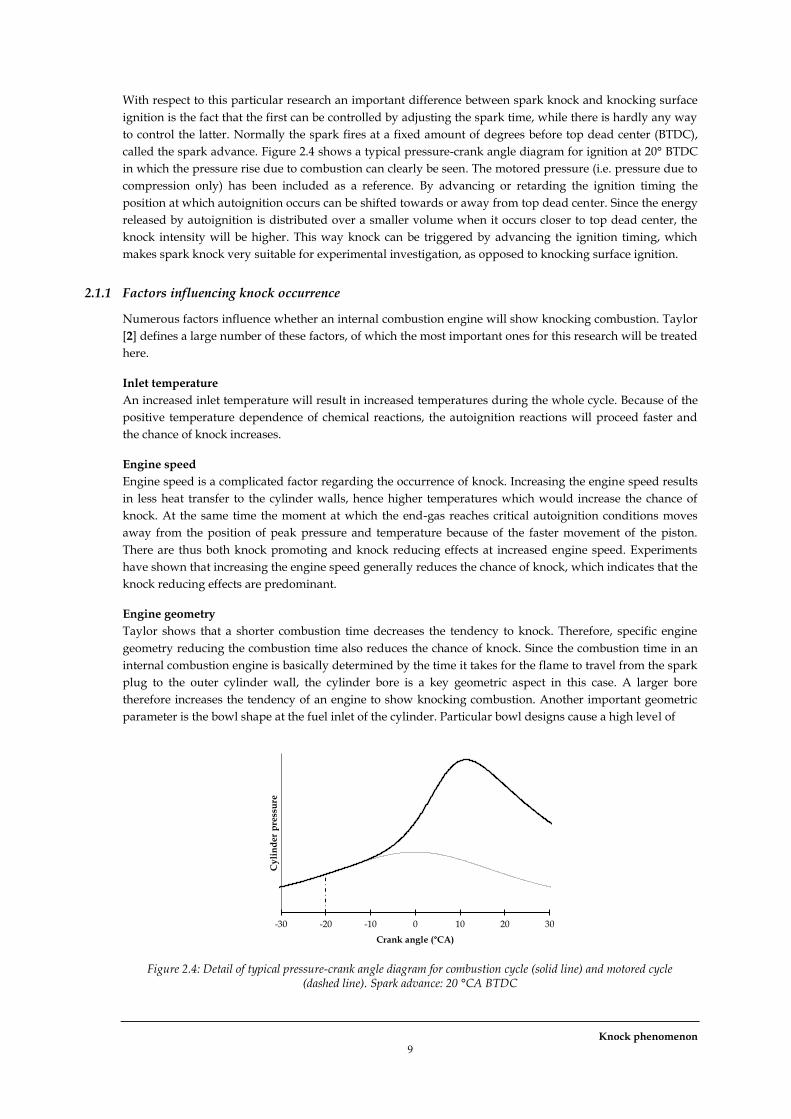
With respect to this particular research an important difference between spark knock and knocking surface

ignition is the fact that the first can be controlled by adjusting the spark time, while there is hardly any way

to control the latter. Normally the spark fires at a fixed amount of degrees before top dead center (BTDC),

called the spark advance. Figure 2.4 shows a typical pressure-crank angle diagram for ignition at 20° BTDC

in which the pressure rise due to combustion can clearly be seen. The motored pressure (i.e. pressure due to

compression only) has been included as a reference. By advancing or retarding the ignition timing the

position at which autoignition occurs can be shifted towards or away from top dead center. Since the energy

released by autoignition is distributed over a smaller volume when it occurs closer to top dead center, the

knock intensity will be higher. This way knock can be triggered by advancing the ignition timing, which

makes spark knock very suitable for experimental investigation, as opposed to knocking surface ignition.

2.1.1 Factors influencing knock occurrence

Numerous factors influence whether an internal combustion engine will show knocking combustion. Taylor

[2] defines a large number of these factors, of which the most important ones for this research will be treated

here.

Inlet temperature

An increased inlet temperature will result in increased temperatures during the whole cycle. Because of the

positive temperature dependence of chemical reactions, the autoignition reactions will proceed faster and

the chance of knock increases.

Engine speed

Engine speed is a complicated factor regarding the occurrence of knock. Increasing the engine speed results

in less heat transfer to the cylinder walls, hence higher temperatures which would increase the chance of

knock. At the same time the moment at which the end-gas reaches critical autoignition conditions moves

away from the position of peak pressure and temperature because of the faster movement of the piston.

There are thus both knock promoting and knock reducing effects at increased engine speed. Experiments

have shown that increasing the engine speed generally reduces the chance of knock, which indicates that the

knock reducing effects are predominant.

Engine geometry

Taylor shows that a shorter combustion time decreases the tendency to knock. Therefore, specific engine

geometry reducing the combustion time also reduces the chance of knock. Since the combustion time in an

internal combustion engine is basically determined by the time it takes for the flame to travel from the spark

plug to the outer cylinder wall, the cylinder bore is a key geometric aspect in this case. A larger bore

therefore increases the tendency of an engine to show knocking combustion. Another important geometric

parameter is the bowl shape at the fuel inlet of the cylinder. Particular bowl designs cause a high level of

Figure 2.4: Detail of typical pressure-crank angle diagram for combustion cycle (solid line) and motored cycle

(dashed line). Spark advance: 20 °CA BTDC

-30 -20 -10 0 10 20 30

Cy

lin

der

pre

ssu

re

Crank angle (°CA)

Literature study 10

turbulence, increasing the flame speed and thus reducing combustion time. High turbulence bowls decrease

the knock tendency of an engine. Finally also the piston shape can influence the occurrence of engine knock.

So called squish design pistons have been designed to cause a radial flow directed to the center of the

cylinder during the compression stroke, see figure 2.5. This causes both an increase in turbulence and a

cooling effect, thus combustion time will reduce and autoignition reactions will proceed slower. This way

these particular pistons reduce the chance of knock.

Air/fuel ratio

Both lean and rich combustion (i.e. combustion with respectively a surplus and a shortage of oxygen

compared to the stoichiometric situation) result in an increased time required for the autoignition reactions

because of lower temperatures in the cylinder. In the lean case this is caused by the cooling effect of the

excessive air, hence lower temperatures in the cylinder. In the rich case the heat release is lower because of

incomplete combustion of the fuel. In both cases this will decrease the chance of knock.

Compression ratio

A higher compression ratio results in a larger temperature increase in the cylinder due to the compression

stroke. Again a higher temperature will result in faster autoignition reactions, thus a higher chance of knock.

An increased compression ratio will therefore increase the knock tendency of an engine.

Fuel composition

Fuels of different chemical composition may have different knock tendencies. First, different fuels may have

different burning velocities. As was mentioned before Taylor [2] indicates that higher burning velocities will

reduce the chance of knock. Autoignition chemistry (see paragraph 2.4) differs from one fuel to another as

well and may play an even more important role in the knock tendency of a fuel. A lot of experimental

research has been performed to classify different fuels based on their knock resistance, see also paragraph 0.

The effect of fuel composition however remains a complicated matter and is one of the main subjects of this

research.

2.2 Knock modeling

Knock modeling requires two types of modeling: one for engine geometry and one for the chemical

behavior of the gas. Combined they can predict the pressure and temperature of the gas during the engine

cycle, which is used in the chemical model to determine possible knock occurrence. Many different types of

models have been developed to predict engine performance in general and knock occurrence in specific. The

difference between these models can be either in the amount of detail with which the flow and the

combustion process is simulated or in what type of model is used for knock prediction. This paragraph

gives an overview of the different methods, which is used to determine which models are most suitable.

Figure 2.5: Example of a squish design pistion. Arrows indicate squish motion.

Knock modeling 11

2.2.1 Geometry models

Two usual ways of incorporating the engine geometry in an internal combustion model could be found in

the literature. The most obvious one is creating a 3D model of the cylinder and connected intake and

exhaust channels which can be used for analysis using computational fluid dynamics (CFD). The more

preferred way however seems to be the use of zero-D models [3]. Both methods will be discussed in more

detail.

Three-dimensional modeling

The basic concept of three-dimensional analysis of an internal combustion engine is meshing the geometry,

which allows for solving the governing equations of mass, momentum and energy conservation in discrete

points within the domain. In this way a highly detailed flow field within the cylinder can be calculated,

including turbulence effects. Furthermore, the three-dimensional approach allows for detailed flame

calculations using turbulent combustion models. Taking all this into account it is clear that three-

dimensional modeling is the preferred way if detailed modeling of the flow is required, but it comes at the

cost of high computational requirements. Therefore with today‟s computational power 3D models are

generally combined with less extensive knock models, such as reduced chemical kinetics (see paragraph

2.2.2). Ge et al. [4] propose to reduce the number of grid points by grouping thermodynamically similar cells

to reduce the computation time. Their research shows that this method can provide accurate results at

relatively low computational expense. Lecocq et al. [5] use a different approach, combining detailed flow

computations with tabulated kinetics: by calculating relevant chemical parameters for autoignition

beforehand using a detailed chemical mechanism and storing them in a database the chemical computations

do not have to be performed during the flow computations. This model proves to be able to simulate knock

and preignition. It was however not validated by any experimental results.

Three-dimensional models require detailed geometry information of the engine cylinder and piston for

creating the computational mesh, performance data like engine speed for determination of the cylinder

volume, valve timing for proper simulation of the intake and exhaust flow and boundary conditions like

inlet pressure, inlet temperature and wall temperature. The output of these models can consist of detailed

flow paths including turbulence data and temperature and pressure distributions over the cylinder.

Zero-dimensional modeling

The distinctive feature of a zero-dimensional model is the fact that the cylinder geometry is not taken into

account explicitly like in 3D modeling. Instead, relevant engine parameters like bore, stroke, speed and

compression ratio are used to determine the instantaneous cylinder volume. This value is subsequently used

for calculating temperatures and pressure in the cylinder. The method therefore assumes uniform conditions

throughout the zones defined in the cylinder. This makes the predictive capability of this approach limited,

but according to Soylu and Van Gerpen [6] it can be very accurate by adjusting particular coefficients in the

correlations to match experimental data. The great advantage of zero-dimensional models is therefore the

fairly accurate results at a fraction of the computational expense of 3D modeling. Furthermore this leaves

room for using it in combination with a detailed chemical kinetics mechanism, see paragraph 2.2.2.

The work of Rassweiler and Withrow [7] has given rise to the development of two zone zero-dimensional

models. They found that the increase in pressure resulting from combustion is proportional to the burnt

mass fraction of the fuel-air mixture in the cylinder. This implies that by dividing the cylinder volume in a

burnt and unburnt zone, the cylinder pressure can be calculated analytically when a correlation for the

burning rate can be found or vice versa. An often cited work in this field is that of Attar [8] who used a two

zone zero-dimensional model combined with detailed chemical kinetics to predict engine knock for

methane-hydrogen mixtures. The model is able to predict knock for mixtures of natural gas and hydrogen

and shows good agreement with experimental data, except at hydrogen fractions exceeding approximately

70 vol%.

Zero-dimensional models require basic information of the cylinder and piston size and engine speed for

determining the volume of the cylinder and initial conditions like intake pressure and temperature. The

output of these models can consist of average temperatures and pressures in the cylinder.

Literature study 12

2.2.2 Knock models

Soylu [3] distinguishes between three different kinds of knock models: those based on empirical ignition

delay correlations, those based on detailed chemical kinetic models and those based on reduced models.

Each one will be treated in more detail. The use of a knock criterion based on enthalpy of combustion is

discussed as well. All models require temperature and pressure of the gas as input. The detailed and

reduced chemical kinetic models require gas composition as well.

Ignition delay correlations

This method, also known as the knock integral approach, uses an autoignition correlation which has to be

derived by fitting a temperature and pressure dependent function to experimental data. Livengood and Wu

[9] have derived an integral function which allows for determination of the crank angle at which knock

starts to occur:

(2.1)

Here θk is the crank angle at which knock starts to occur and τ is the autoignition correlation. An example of

such a correlation is the one used by Soylu [3]:

(2.2)

In this equation p is pressure, Tu is the temperature of the unburnt gas and X1, X2 and X3 are experimental

constants. With this correlation Soylu was able to predict the knock occurrence crank angle within 1 °CA of

the experimental value. It is however clear experiments are a necessity when using these ignition delay

correlations, since either a complete new function or several experimental constants have to be determined

for every engine and every fuel. Furthermore, it is characteristic that this method only gives output related

to the time of knock occurrence and does not take into account details of the combustion reactions.

Detailed chemical kinetics

Models using detailed chemical kinetics consist of an extensive amount of elementary reactions linked to the

combustion process. Included are the chemical and thermodynamic properties of all species1 considered.

This way specific software can calculate nearly every detail of the combustion process, such as reaction

rates, chemical composition, temperature and pressure. These models are therefore well suited to simulate

autoignition reactions in engine conditions (see also paragraph 2.4 about chemical kinetics), and thus to

predict knock occurrence. A huge advantage of these models is that the chemical kinetics databases are

widely available in the literature. The downside however is that because of the extensive amount of

reactions and species the methods require a relatively large amount of computation time.

One of the most well known mechanisms developed for this purpose is GRI Mech 3.0 [10], consisting of 325

reactions and 53 species up to hydrocarbons with a carbon number of three. Close inspection however

learns that the important low temperature oxidation reactions treated in paragraph 2.4 are not included in

this particular mechanism. Since these reactions are believed to be the basis of knock occurrence, this

mechanism could be less suitable for knock prediction. An alternative could be the mechanisms C3_41 and

nC5_50 developed by the National University of Ireland [11][12], which include respectively 124 and 293

species, approximately 700 and 1500 reactions and species up to hydrocarbons with a carbon number of

respectively three and five. These mechanisms do include all important reactions treated in paragraph 2.4.

Reduced chemical kinetics

To decrease the required computational effort of the detailed chemical kinetics approach it is possible to

reduce the reaction mechanism to reactions relevant for autoignition. An example is the work of Cowart et

al. [13] who compare a reduced kinetic model of 19 reactions with a detailed model of 1303 reactions. The

1 Atoms, molecules, etc. subjected to a chemical process

Knock modeling 13

output parameters are equal to models based on detailed chemical kinetics, but contain details about less

species. One of the reduction steps consists of grouping together certain species, which will react according

to one specific reaction. It is interesting to see that some, but not all of the autoignition reactions treated in

paragraph 2.4 are included in the reduced mechanism. This might be due to the grouping procedure.

Cowart et al. find that in the case of pure fuels both the reduced and the detailed chemical kinetics model

can predict the time of onset of knock accurately. The reduced mechanism however had to be calibrated by

two experimental runs with iso-octane and n-pentane on the particular engine. The great advantage of the

method is that because of its low computational expense it can be more easily combined with for example a

detailed flow model. Depending on whether the flow or the chemistry is the determining factor in a specific

application, the decision could therefore be made between a reduced and a detailed mechanism.

Knock criterion

Karim and Gao [14] have defined a knock criterion based on the consideration that the unburnt gas has to

release sufficient energy to cause knock. This is expressed in the ratio of energy released by the unburnt gas

up to time t and the total energy to be released by flame propagation, combined with the ratio of the

instantaneous cylinder volume and the cylinder volume at the start of the compression stage. Attar [8] has

rewritten the knock criterion using specific enthalpies:

(2.3)

Here is the specific enthalpy of combustion of the fresh fuel-air mixture, mu is the mass of unburnt gas at

time t, Vcyl is the cylinder volume at time t, LHV is the lower heating value of the fuel, mfuel,0 is the total mass

of fuel in the cylinder at the start of the process and Vcyl,bdc is the cylinder volume at bottom dead center.

Based on experiments Karim and Gao have derived a critical value of this criterion. At this value Karim and

Gao have found knock to occur and although they are inconclusive about the exact definition of knock, it is

most probably related to the intensity at which knock becomes audible. The advantage of this dimensionless

approach is that the same critical value should be found for every engine and every gas, regardless of engine

geometry and gas composition.

2.2.3 Engine correlations

A large number of correlations between in-cylinder conditions, engine operating conditions and physical

phenomena occurring in the cylinder have been published in the literature. A number of these correlations

can be used in knock modeling. For this reason correlations for the heat transfer coefficient to the cylinder

wall, the heat release rate due to combustion and the laminar flame speed are discussed in this paragraph.

Wall heat transfer coefficient

Most internal combustion engines are cooled during operation, which results in a large temperature

difference between the cold cylinder wall and the hot gases in the cylinder. Depending on the operating

speed of the engine this could result in significant heat transfer from the gas to the cylinder wall.

Heywood [1] treats several correlations for wall heat transfer in cylinders of spark ignition engines. As

suggested by Attar [8] and endorsed by Mohammedi and Yaghoubi [15] the most appropriate one for this

application is the correlation derived by Woschni [16]:

(2.4)

In which hc is the heat transfer coefficient, B is the bore of the cylinder, p is the pressure at time t, T is the

temperature at time t and w is the average cylinder gas velocity defined by:

Literature study 14

(2.5)

In which is the mean piston speed, Vd is the displaced volume at time t, T0, p0 and V0 are respectively the

temperature, pressure and volume at the start of compression, p is the pressure at time t and pm is the

motored pressure (i.e. pressure without combustion) at time t. Finally, C1 and C2 are coefficients depending

on the phase of the cycle; C1 has a constant value of 2.28, while C2 is zero during compression and 3.24e-3

during combustion and expansion.

Combustion heat release rate

Chmela et al. [17] have derived an analytical formula for the combustion heat release rate of a turbulence

controlled mixing process, in which all turbulence related terms have been combined in one model

parameter C:

(2.6)

Here Qcomb is the heat released by combustion, C is a turbulence factor, LHV is the lower heating value of the

fuel, λ is the air-fuel equivalence ratio, AFRstoich is the stoichiometric air-fuel ratio, ρb is the density of the

burnt gas, SL is the laminar flame speed and mfuel,i is the mass of fuel in the cylinder prior to combustion.

Chmela et al. [17] have compared their relation to experiments performed on two engines; one with a low

and one with a high turbulence combustion chamber. In the latter case increased turbulence is created by

progressive intake valve opening. Important conclusions are that the value of the turbulence factor C can be

taken as a constant throughout the combustion phase and the value can be both larger and smaller than 1.

Laminar flame speed

Flame speed is defined as the speed at which the flame front moves through the unburnt mixture. It is a

critical combustion property when investigating engine knock, because it directly influences combustion

phasing and thus the conditions of the unburnt gases.

Metghalchi and Keck [18] have performed much cited research carrying out a large number of flame speed

measurements using different equivalence ratios over a wide temperature and pressure range. It has been

shown that the actual flame speed can be accurately approximated by relating it to a reference flame speed

using a correlation of the following form:

(2.7)

Here is the laminar flame speed, the laminar flame speed at reference conditions, Tu and p the

temperature and pressure of the unburnt gas at time t, Tref and pref the reference temperature and pressure

and α and β are experimental coefficients.

The last term is a correction for diluents, where f is the mass fraction of the diluents. Using this correlation it

is possible to predict the flame speed at certain pressure and temperature conditions once the flame speed at

reference conditions Tref = 298 K and pref = 1 atm is known. Based on a best fit of the experimental results

Metghalchi and Keck suggest the following relations for α and β as a function of equivalence ratio :

(2.8)

(2.9)

Experimental knock research 15

2.3 Experimental knock research

Because the model developed in this research is validated with experiments this paragraph first gives a

short description of two methods of experimental knock detection. Next, two experimental ways of

classifying fuels on their knock resistance are treated. These are useful during the experiments as well as for

comparing the results of the model to existing knock classifications.

2.3.1 Knock detection

There are several ways of detecting knock based on a measured pressure signal. Rahmouni et al. [19]

distinguish between direct evaluation from cylinder pressure, filtered pressure analysis and pressure

derivatives analysis. Because of the large amount of methods available, only the most important ones will be

treated in more detail.

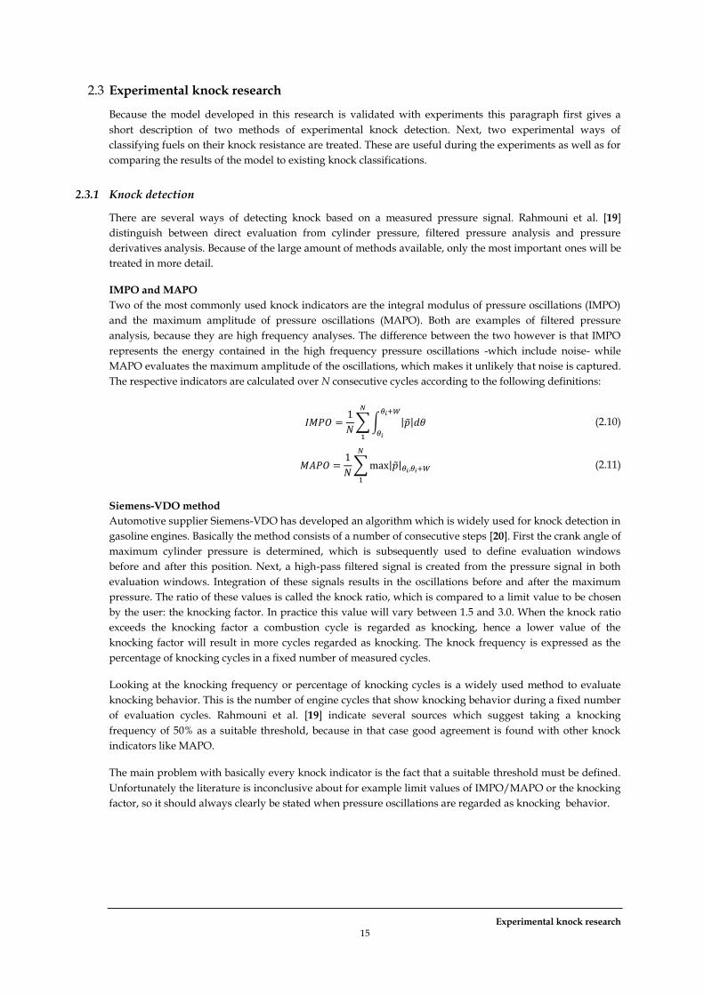
IMPO and MAPO

Two of the most commonly used knock indicators are the integral modulus of pressure oscillations (IMPO)

and the maximum amplitude of pressure oscillations (MAPO). Both are examples of filtered pressure

analysis, because they are high frequency analyses. The difference between the two however is that IMPO

represents the energy contained in the high frequency pressure oscillations -which include noise- while

MAPO evaluates the maximum amplitude of the oscillations, which makes it unlikely that noise is captured.

The respective indicators are calculated over N consecutive cycles according to the following definitions:

(2.10)

(2.11)

Siemens-VDO method

Automotive supplier Siemens-VDO has developed an algorithm which is widely used for knock detection in

gasoline engines. Basically the method consists of a number of consecutive steps [20]. First the crank angle of

maximum cylinder pressure is determined, which is subsequently used to define evaluation windows

before and after this position. Next, a high-pass filtered signal is created from the pressure signal in both

evaluation windows. Integration of these signals results in the oscillations before and after the maximum

pressure. The ratio of these values is called the knock ratio, which is compared to a limit value to be chosen

by the user: the knocking factor. In practice this value will vary between 1.5 and 3.0. When the knock ratio

exceeds the knocking factor a combustion cycle is regarded as knocking, hence a lower value of the

knocking factor will result in more cycles regarded as knocking. The knock frequency is expressed as the

percentage of knocking cycles in a fixed number of measured cycles.

Looking at the knocking frequency or percentage of knocking cycles is a widely used method to evaluate

knocking behavior. This is the number of engine cycles that show knocking behavior during a fixed number

of evaluation cycles. Rahmouni et al. [19] indicate several sources which suggest taking a knocking

frequency of 50% as a suitable threshold, because in that case good agreement is found with other knock

indicators like MAPO.

The main problem with basically every knock indicator is the fact that a suitable threshold must be defined.

Unfortunately the literature is inconclusive about for example limit values of IMPO/MAPO or the knocking

factor, so it should always clearly be stated when pressure oscillations are regarded as knocking behavior.

Literature study 16

2.3.2 Fuel knock resistance classification

Klimstra et al. [21] give an overview of different classification methods for the knock resistance of gaseous

fuels, among which are the methane number method and the knock-limited spark timing method. The first

is the most widely used method of classification for gaseous fuels, while the latter is of great importance for

this particular research. Both will therefore be treated in more detail.

Methane number

The methane number method was developed by the Austrian company AVL. Based on a large number of

experiments in an engine with variable compression ratio, the compression ratio at which knock occurs

(knock limit compression ratio, KLCR) could be determined for different fuels [22]. The KLCR has been

determined for stoichiometric mixtures of methane and hydrogen. Subsequently the methane number has

been defined as the percentage of hydrogen in the mixtures, hence every value of the methane number

corresponds to an experimentally determined KLCR. By determining the KLCR of an arbitrary fuel and

comparing this to the results found for methane-hydrogen mixtures, a methane number can be allocated to

every fuel. Should a fuel prove to be more knock resistant than methane, the methane number can be

determined by comparing the knock resistance to that of methane-carbondioxide mixtures. In this case the

percentage of CO2 in the mixture is added to 100 to give the proper methane number.

Throughout the world engine manufacturers have developed mathematical correlations to determine the

methane number of fuels, hereby reducing the need for expensive and time consuming experiments. The

methane number has become the most widely accepted classification for the knock resistance of fuels, which

is reflected by the fact that most manufacturers of gas fueled engines specify a minimum required methane

number at which their engines can operate safely.

Knock-limited spark timing

Another way of determining the knock resistance of a fuel is advancing the spark timing of an engine up to

a level where knock just starts to occur, a state known as knock-limited combustion. The related spark

advance is likewise known as knock-limited spark timing, on which basis fuels can be classified regarding

knock resistance. As was explained in paragraph 2.1 the ignition timing has to be advanced to force the

occurrence of knock, hence more knock resistant fuels will have a more advanced knock-limited spark

timing.

This method is worth referring to for two reasons. First, most engine-management systems use this method

for knock control, which implies that the experimental and real situation will be much alike. Second, this

method gives the possibility to perform experiments on regular engines, instead of requiring rapid

compression machines or other specific test equipment.

2.4 Chemical kinetics

According to Warnatz et al. [23] the onset of autoignition is almost exclusively governed by chemical

kinetics. For this reason it is important to get acquainted with the chemical reactions leading to autoignition.

This paragraph gives an overview of the reactions which are believed to be the cause of knock and also

check whether the chemical mechanisms used in this research are capable of modeling these reactions.

Atoms or molecules with unpaired electrons are called free radicals. They are generally highly reactive and

play an important role in combustion and knock phenomena. In reaction equations they are generally

denoted by a dot at the side of the atom with an unpaired electron. Warnatz et al. [23] indicate that

combustion at high temperatures is dominated by the following chain branching reaction producing

hydroxyl (HO) radicals. The hydrogen radical involved results from preliminary reactions.

(2.12)

Due to the large activation energy of this reaction it can however not explain autoignition at temperatures

below 1200 K, while experiments show that autoignition occurs at temperatures as low as 800-900 K. One of

Chemical kinetics 17

the suggested mechanisms which governs the ignition process by forming hydroxyl radicals through

another route is:

(2.13)

(2.14)

(2.15)

(2.16)

(2.17)

Equation (2.13) describes how hydrocarbon radicals react with oxygen to peroxy1 radicals. The peroxy

radicals extract an additional hydrogen atom from other hydrocarbons, forming hydroperoxy compounds

(2.14). Finally, in (2.15) the hydroperoxy compounds decompose into an oxy radical and a hydroxide radical.

In case of higher hydrocarbon radicals there might be a possibility to form a cyclic compound2 after reaction

(2.13), in which case the molecule abstracts a hydrogen molecule from itself (2.16). This ring can

subsequently decompose in an aldehyde or ketone and a hydroxide radical, as shown in (2.17). Because the

internal collision rate is much larger than the external one, external hydrogen abstraction (2.14) is much

slower and can therefore not explain autoignition phenomena. Internal abstraction on the other hand seems

to be a plausible explanation.

Although Warnatz et al. propose even another mechanism, Battin-Leclerc et al. [24] and Zádor et al. [25]

endorse internal hydrogen abstraction and subsequent decomposition as a main mechanism for

autoignition. Furthermore, several other reactions are pointed out by Zádor et al. which play an important

role in the autoignition process:

(2.18)

(2.19)

(2.20)

(2.21)

These reactions describe how hydroperoxy radicals (HO2) contribute to the reaction mechanism of (2.13) -

(2.17) by producing either reactive hydroxyl (HO) radicals or one of the intermediate reactants ROOH and

RH.

According to Zádor et al. (2.16) - (2.21) are the key reactions for low temperature combustion and

autoignition. The mechanism used for predicting knock should therefore include these reactions to be able

to perform accurate simulations. In this research the mechanisms GRI Mech 3.0[10], C3_41 [11] and nC5_50

[12] have been used. To see if these mechanism suit the theory described above, it has been checked if above

reactions are included:

(2.22)

(2.23)

(2.24)

(2.25)

Equations (2.22) - (2.25) describe the internal hydrogen abstraction mechanism involving ethane from the

nC5_50 mechanism, corresponding to (2.13), (2.16) and (2.17). Similar reactions are included for propanes,

butanes and pentanes. As was mentioned before, hydrocarbon radicals need to form a stable ring to allow

1 Molecule containing an oxygen-oxygen single bond 2 Series of atoms connected to form a stable ring

Literature study 18

for internal hydrogen abstraction which is not possible for methane. Above mechanism is therefore not

included for methane, but the external hydrogen abstraction process described by (2.13) - (2.15) is. The

C3_41 mechanism contains these reactions as well, except for (2.25). GRI Mech 3.0 does not include any of

these reactions.

The other important autoignition reactions (2.18) - (2.21) are also included in the nC5_50 and C3_41

mechanisms, for example these methane related reactions:

(2.26)

(2.27)

(2.28)

(2.29)

Here (2.26) corresponds to (2.19), while subsequent reaction (2.26) and (2.27) together correspond to (2.18).

Furthermore, (2.28) and (2.29) correspond to (2.20) and (2.21) respectively. Similar reactions are also

included for ethane, propane, butanes and pentanes. GRI Mech 3.0 includes reaction (2.29) only.

The chemical kinetics of knock phenomena in hydrogen have been investigated less thoroughly compared

to conventional hydrocarbon fuels. Huang et al. [26] however indicate that in methane-hydrogen mixtures at

low temperatures the reaction between hydrogen and methylperoxy radicals has a combustion promoting

effect by contributing additional hydrogen radicals:

(2.30)

Furthermore subsequent decomposition of the methylhydroperoxide results in a hydroxyl radical, which is

the most important species in the low temperature hydrocarbon reactions described above:

(2.31)

This reaction sequence is incorporated in the nC5_50 and C3_41 mechanisms up to respectively butane and

propane hydrocarbons. GRI Mech 3.0 does not include these reactions. Based on the fact that the most

important autoignition reactions are included in the nC5_50 and C3_41 mechanism, they seem suitable

mechanisms for performing knocking simulations. The suitability of GRI Mech 3.0 is doubtful.

2.5 Final considerations

Based on the literature study the most suitable approach for this research has been chosen. One of the major

considerations in this case was the fact that one of the research partners is involved in developing detailed

chemical mechanisms as discussed in paragraph 2.2.2. This suggests developing a model incorporating

detailed chemical kinetics. Furthermore, since the model shall be used in future to investigate a large

number of engines and gas compositions rather than a small number of cases, the simulations should

preferably not be very time expensive. Finally there is also a limitation raised by the software available at

the research partners.

Considering all this, a zero-dimensional two zone model seems the most appropriate solution, since it is able

to incorporate detailed chemical kinetics mechanisms, is time inexpensive and can be created using basically

every basic programming language. In the following chapter the development of this model will be treated

in more detail.

Model description 19

3 Research method

A zero dimensional numerical model has been developed based on the work by Attar [8]. This chapter

describes the basics of the zero dimensional two-zone model. Furthermore the experimental setup as well as

the experimental procedure used for validating the model are treated.

3.1 Model description

To give a quick overview of the model this paragraph starts with a short general description of the model.

The fundamental equations from which the development of the model has started will be treated as well.

Finally this paragraph describes the software used for development of the model.

3.1.1 General description

In the approach of Attar the volume of the cylinder is assumed to consist of two zones during the

combustion process: a zone of burnt gas and a zone of unburnt gas, see figure 3.1. The way the volume is

divided geometrically over these two zones will not be taken into account, which makes the model

essentially zero-dimensional. Furthermore, the following assumptions are applied to the two zones.

Both zones are homogeneous regarding composition and density and uniform regarding

temperature and pressure

Pressure is uniform throughout the cylinder and equal to the pressure of the burnt zone

The thickness of the flame separating the two zones is negligible

Both burnt and unburnt gas behave like ideal gases

Blow-by/leakage is negligible

The goal is to simulate the compression, combustion and expansion stage of the combustion cycle as

accurate as seems appropriate.

Figure 3.1: Schematic diagram of the two-zone model [8]

Research method 20

3.1.2 Fundamental equations

The actual model consists of a set of equations, solved consecutively in an iterative loop to determine the

properties of each zone at specific points in time. These equations will be derived here from fundamental

concepts.

Conservation equations

Three fundamental principles of physics are conservation of mass, momentum and energy. Applying the

principle of mass conservation to this specific situation gives:

(3.1)

In which mcyl is the total mass in the cylinder and mu and mb are the mass of unburnt and burnt gas

respectively. Since the total mass in the cylinder is constant during the simulated cycle, taking the time

derivative of (3.1) leads to:

(3.2)

Conservation of volume is not a fundamental principle, but definitely a constraint for this two zone model:

(3.3)

Equation (3.3) states that the sum of the burnt and unburnt gas volume is equal to the total cylinder volume.

When turbulence effects are neglected the gas within the cylinder essentially is a quiescent flow, so

application of the equations of momentum conservation is redundant in this case. Energy conservation on

the other hand can be expressed by the first law of thermodynamics in differential form:

(3.4)

In which U is the internal energy of the system, Q the heat supplied to the system and W the work done by

the system. Expressing the internal energy in the specific internal energy u and taking the time derivative

leads to:

(3.5)

(3.6)

Equations of state

The state of a system in equilibrium can be described by the thermodynamic state variables pressure,

density, temperature, internal energy, enthalpy and entropy. For an ideal gas the relations between these

variables are given by the thermal (3.7) and caloric (3.8)(3.9) equations of state.

(3.7)

(3.8)

(3.9)

In which p is pressure, V is volume, m is mass, R is a specific gas constant, T is temperature, u is specific

internal energy, h is specific enthalpy and cv and cp are specific heat capacity at constant volume and

constant pressure respectively.

Model description 21

Applying the thermal equation of state (3.7) to both the burnt and unburnt zone and recognizing that the

pressure is uniform over the cylinder gives:

(3.10)

(3.11)

Combining these equations and substituting (3.3) gives the following equation for the cylinder pressure:

(3.12)

It should be noted that for an ideal gas the following relation holds between R, cv and cp.

(3.13)

Energy equation

Part of the heat supplied to the system consists of heat transfer to and from the wall of the cylinder, which in

accordance with Attar [8] is assumed to be solely convective. The heat term in (3.4) can therefore be

expressed using Newton‟s law of cooling:

(3.14)

In which hc is the heat transfer coefficient, A is the surface area through which heat transfer takes place and

ΔT is the temperature difference between the gas and the cylinder wall.

Furthermore there is heat from chemical reactions in the system, which can be expressed as:

(3.15)

In this equation V is the volume of the system, N is the number of species in the system, is the rate of

production of species i, Mi is the molecular weight of species i and ui is the specific internal energy of species

i. The minus sign is required to make sure that destruction of species ( negative) results in a positive

energy change and the opposite occurs for creation of species.

The incremental work done by the system can be expressed by the system pressure multiplied by the change

in volume of the system, hence:

(3.16)

Finally, there will be a contribution to the energy equation describing the change in total energy of the

system due to flame propagation, which essentially occurs by mass transfer from one system to another.

This term can therefore be expressed as:

(3.17)

Here h is the specific enthalpy of the system and

is the mass transfer rate across the flame.

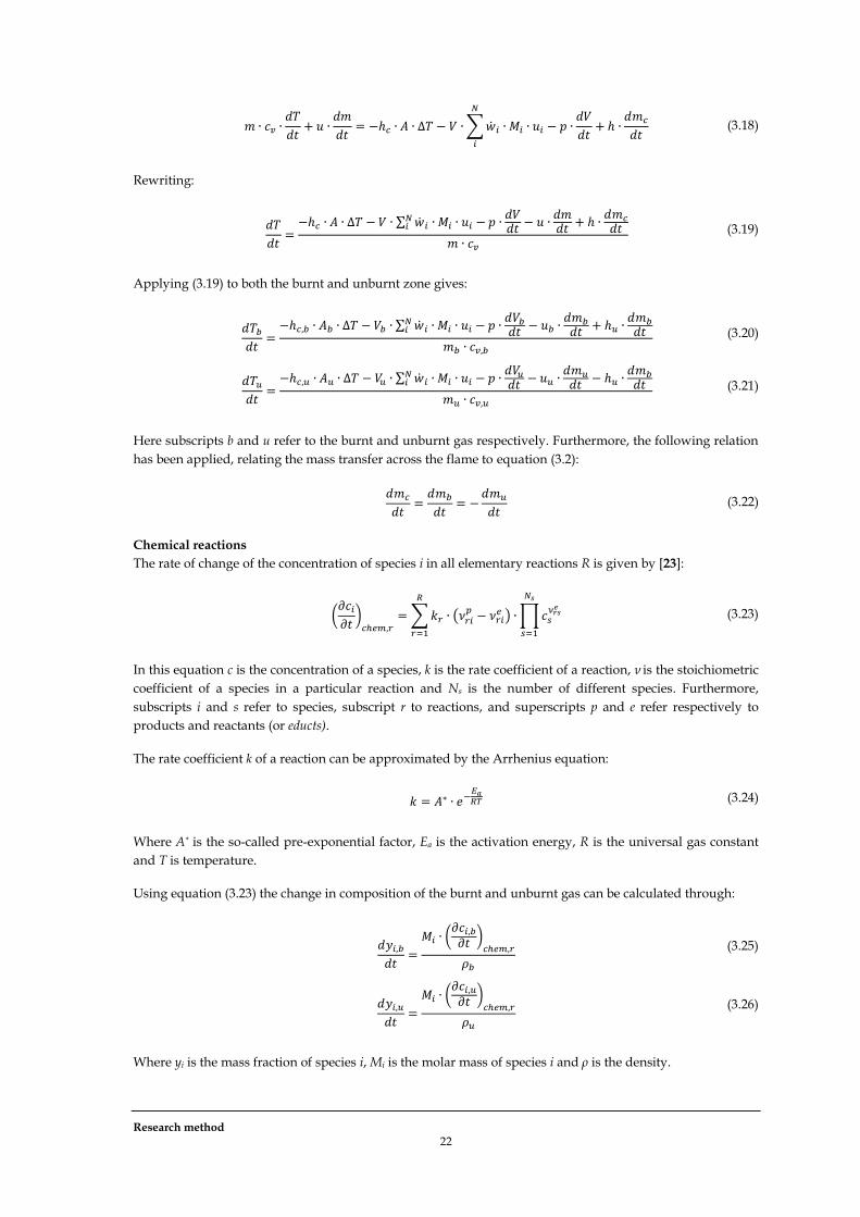
Substituting equations (3.6), (3.8) and (3.14) - (3.17) into (3.4) gives:

Research method 22

(3.18)

Rewriting:

(3.19)

Applying (3.19) to both the burnt and unburnt zone gives:

(3.20)

(3.21)

Here subscripts b and u refer to the burnt and unburnt gas respectively. Furthermore, the following relation

has been applied, relating the mass transfer across the flame to equation (3.2):

(3.22)

Chemical reactions

The rate of change of the concentration of species i in all elementary reactions R is given by [23]:

(3.23)

In this equation c is the concentration of a species, k is the rate coefficient of a reaction, ν is the stoichiometric

coefficient of a species in a particular reaction and Ns is the number of different species. Furthermore,

subscripts i and s refer to species, subscript r to reactions, and superscripts p and e refer respectively to

products and reactants (or educts).

The rate coefficient k of a reaction can be approximated by the Arrhenius equation:

(3.24)

Where A* is the so-called pre-exponential factor, Ea is the activation energy, R is the universal gas constant

and T is temperature.

Using equation (3.23) the change in composition of the burnt and unburnt gas can be calculated through:

(3.25)

(3.26)

Where yi is the mass fraction of species i, Mi is the molar mass of species i and ρ is the density.

Experimental setup and procedure 23

3.1.3 Software implementation

The backbone of the model is Cantera: an open source software code capable of performing calculations

involving chemical kinetics and thermodynamics. The software allows for creating objects representing a

gas of which composition and physical properties like temperature, pressure and/or density can be

prescribed. Based on these values the software automatically calculates other properties like average

molecular weight, specific enthalpy, specific internal energy and specific heat capacity. Furthermore the

software is able to relate changes in temperature and/or pressure to changes in composition and vice versa

using equilibrium computations. In these cases it is assumed that gases behave according to the ideal gas

law (Equation (3.7) and reaction rates are temperature dependent according to the Arrhenius law (Equation

(3.24)).

The data for the computations such as reaction rate constants and species properties are supplied by a

chemical reaction mechanism and a corresponding database of thermodynamic properties. These are widely

available in the literature and can range up to several hundred species and several thousand reactions. More

extensive mechanisms could give more accurate results, but come at the cost of larger computational

expense.

The Cantera code is implemented in Matlab as a toolbox. This allows for using Cantera commands and objects

in scripts written in Matlab. The scripts make up the actual model described in paragraphs 4.1.1 - 4.1.3.

3.2 Experimental setup and procedure

To validate the results of the model experiments are performed on the reciprocating engine of a combined

heat and power (CHP) unit in the Kiwa Gas Technology laboratory. This paragraph describes the details of

the engine, the data acquisition system, gas compositions used and the experimental procedure.

3.2.1 Engine

Most important engine details can be found in table 3.1. Furthermore the engine is equipped with a

manually adjustable ignition controller, which allows for stepless adjustment of the ignition timing between

7 and 33 °CA BTDC.

Model Mercedes G8V183A Number of cylinders 8 Cylinder configuration 90 °CA V Combustion system Spark ignition Engine type Four stroke cycle Air-fuel ratio Stoichiometric Fuel delivery Carburetor Rated speed 1500 rpm Electric power output 150 kW Bore 128 mm Stroke 142 mm Connecting rod 259.5 mm Total displacement 14.6 L Compression ratio 12 Table 3.1: Test engine specifications

3.2.2 Data acquisition system

During the experiments the following properties of the cylinder are measured and processed in real time:

pressure, crank angle, spark timing and exhaust gas temperature.

Cylinder pressure is measured with a piezoelectric sensor incorporated in a spark plug which replaces the

original spark plug of the cylinder being measured. Two pressure sensors are used; one in a reference

cylinder and one in a cylinder which has the highest average peak pressure during normal operation. The

Research method 24

latter is the cylinder in which knock is expected to occur first. An optical encoder placed on the flywheel of

the engine measures crank angle at a resolution of 0.1 °CA. Spark timing is measured using a current clamp

connected to the electrical conductor between the spark plug and the distributor cap. It is placed at one of

the cylinders in which pressure is measured as well. The exhaust temperatures are measured by

thermocouples placed directly behind the exhaust valves of every cylinder.

A Kistler engine diagnostics system is connected to the engine, processing the incoming pressure, crank

angle and spark time signals. The engine diagnostics system in its turn is connected to a PC equipped with

KiBox Cockpit: software to process data from the diagnostics system in real time. Furthermore, the PC is

connected to the control system of the CHP unit which allows for reading the temperatures of the different

cylinders directly behind the exhaust valves.

3.2.3 Gas compositions

The experiments have been performed with a number of different gas blends, which are blended using

custom made venturi nozzles. The mixture fraction is hence determined by installing the appropriate

venturi. The base gas in these experiments is Groningen quality natural gas (G25, blend no. 1), which is

blended with hydrogen and carbon monoxide. To determine the composition of the natural gas and the

exact mixture fraction the blends are analyzed using gas chromatography. The compositions used in the

experiments can be found in table 3.2.

Blend no.

Mol% 1 2 3 4 5 6 7 8*

CO 0 0 0 0 0 0 0 6.86 H2 0 2.618 6.786 10.394 13.673 19.682 27.433 24.91 He 0.049 0.046 0.044 0.043 0.040 0.037 0.032 0.03 N2 13.952 13.692 13.183 12.733 12.408 11.753 10.497 9.90 CH4 81.514 79.303 75.845 72.834 70.080 65.005 58.998 55.40 CO2 1.056 1.028 0.980 0.953 0.894 0.837 0.723 0.70 C2H6 2.810 2.720 2.596 2.499 2.386 2.205 1.902 1.85 C3H8 0.388 0.374 0.357 0.344 0.328 0.303 0.262 0.26 iC4H10 0.064 0.061 0.059 0.056 0.054 0.050 0.043 0.04 nC4H10 0.073 0.070 0.067 0.064 0.061 0.056 0.049 0.04 C5H10 0.018 0.017 0.016 0.016 0.015 0.014 0.012 <0.01 Table 3.2: Gas compositions used in the experiments (*composition analysis performed at lower accuracy)

3.2.4 Experimental procedure

The procedure is started by adjusting the spark timing of the engine to 10 °CA BTDC. This way the chance

of knock occurring immediately after the blended gas is fed to the engine is negligible. After a run in period

of approximately 10 minutes the spark timing is adjusted manually by steps of approximately 1.0 °CA.

During the procedure the knock frequency is calculated continuously using the Siemens-VDO method

described in paragraph 1.1. At every spark timing knock frequency and pressure data are saved over a

course of 200 cycles, while the exhaust temperatures are logged continuously. The knock-limited spark

timing is defined when the knocking frequency has risen to an average value of 50%. This marks the end of

the procedure.

Because the CHP unit supplies an important part of heat and electricity in the building and is not intended

primarily for experiments, damaging the engine by heavy knock should be prevented at all times. For this

reason the Siemens-VDO knock indicator is programmed at its most sensitive setting. In case of the software

used this implies a knocking factor of 1.5. Furthermore the knocking frequency is calculated over 50

consecutive cycles, which is the default setting.

The cycle-to-cycle variations in the cylinders make it difficult to compare the experimental data to the

output of the model. For this reason the average values of the 200 recorded cycles are calculated and used to

validate the model.

Experimental setup and procedure 25

Figure 3.2: Schematic overview of the experimental setup

Figure 3.3: Data acquisition Figure 3.4: Test engine

Figure 3.5: Current clamp Figure 3.6: Carburetor

Air Carburetor

Blendable

gas

Venturi

Engine Engine

control

system

Ambient

conditions

measurement

system

Motor

diagnostics

system

PC

Natural gas

Exhaust gas

Pressure data

Crank angle data

Spark signal

Temperature data

Motor diagnostics system

Current clamp

Carburetor

Air supply

Gas supply

Engine control system

Results 26

4 Results

Based on the basic two zone model described in chapter 3 a complete knock prediction model has been

developed, which will be described in detail in this chapter. Next, the validation of the model using

experimental results is treated. The model is validated with a comparison based on the methane number as

well. Finally this chapter contains a sensitivity analysis of the model.

4.1 Knock prediction model

This paragraph contains a detailed description of the knock prediction model. The flowchart on the next

page gives a complete overview of the model, which consists of three parts: user input, compression stroke

and combustion phase. Each of these parts will be discussed in more detail in the following subparagraphs.

4.1.1 User input

This subparagraph treats the user input required for the model, which consists of engine data, gas

composition, ambient conditions, laminar flame speed and a turbulence factor.

Engine data

The engine data required for the model can be divided in geometric and operating parameters. The first

category comprises bore, stroke, connecting rod length and compression ratio. Required operating

parameters are engine speed, inlet pressure, cooling water temperature, exhaust gas temperature, manifold

temperature and crankshaft angles at which the valves open and close.

Gas composition

The composition of the gas is required in mole percent. The supported species depend on the mechanism

used. The mechanism nC5_50 for example supports the following common natural gas components: linear

hydrocarbons up to and including pentane, isobutane, nitrogen, carbon dioxide and helium. Furthermore

hydrogen and carbon monoxide are supported as well.

Ambient conditions

The only ambient condition required is the ambient pressure. The fresh mixture is assumed to reach the

temperature of the manifold; hence ambient temperature is not required. The same accounts for humidity,

which is proven to be irrelevant for the simulations (see paragraph 4.5.2).

Laminar flame speed

The laminar flame speed at reference temperature 298 K and reference pressure 1 atm. as defined by

Metghalchi and Keck [18] is required to calculate the effective laminar flame speed during the engine cycle.

It can be calculated using a script included in Cantera, for which the user only needs to supply the

composition of the fresh fuel-air mixture. It should be noted that it is currently not possible to include the

effect on the laminar flame speed of hydrocarbons higher than propane, because the transport database

which is required for the computation is not yet available for the nC5_50 mechanism used. For the

mechanisms capable of simulating up to propane (see paragraph 2.2.2) the transport databases are available.

Turbulence factor

The model requires a turbulence factor as input which is used to determine the heat release rate. Although it

is a theoretically derived constant [17] there is hardly any way to determine the actual value of the factor on

a theoretical basis. It is therefore recommended to use a trial-and-error approach to find the most suitable

turbulence factor for the engine at hand. In this research a turbulence factor of 2.6 has proven to give the

best fit to the experimental results (see paragraph 4.4.1). This value turns out to be in the same order of

magnitude as was determined by the authors of the original paper for two test engines: 0.9 and 1.35 [17].

Knock prediction model 27

Figure 4.1: Model flowchart

Stoichiometric

air-fuel ratio

Amount of

residual gas

Lower heating

value of gas

Engine data

Gas composition

Ambient conditions

Laminar flame speed

Turbulence factor

Amount of fuel

and combustion

air

Initial

temperature

mixture

Motored pressure

and temperature

Create burnt gas

Heat release rate

Burnt and unburnt

mass

Unburnt gas

temperature and

composition

Burnt gas

temperature and

composition

Cylinder pressure

Burnt and unburnt

volume

Knock criterion

Laminar flame

speed

Cylinder volume

Iteration

step

Δθ

Compression stroke Combustion phase

User input

Ignition lag

Results 28

4.1.2 Compression stroke

In this subparagraph the modeling of the compression stroke is treated. It focuses on the way initial

parameters such as the amount of fuel and combustion air are calculated and ends with the equations used

for calculating the pressure and temperature during the compression stroke. These last two parameters are

subsequently input for the combustion phase. Key concept in this case is that there is only a single zone

during the compression stroke.

Amount of residual gas

During the exhaust stroke of the piston burnt gases will leave the cylinder until the in-cylinder pressure is

too small to overcome the pressure losses in the exhaust. Another possibility is that the exhaust valve closes

before this point is reached. In any case an amount of burnt gases will remain in the cylinder: the residual

gas. This will reduce the amount of fresh mixture able to enter the cylinder, as well as increase the

temperature of the mixture in the cylinder.

To calculate the amount of residual gas, first the composition of the burnt gas at the end of the cycle is

approximated by calculating the equilibrium composition using a built-in function of Cantera. Next, the

density of the burnt gas is calculated assuming the gas is at exhaust gas temperature and ambient pressure.

Furthermore the instantaneous cylinder volume at the time the exhaust valve closes can be calculated using

equation (4.14). Multiplying the density by the instantaneous cylinder volume gives the mass of residual gas

in the cylinder.

Stoichiometric air-fuel ratio

Internal combustion engines operate either rich, stoichiometric or lean. This means there is respectively too

little, exactly enough or too much combustion air available for complete combustion. In this perspective

calculating the amount of air required for stoichiometric combustion is a key aspect.

Every combustion reaction has specific stoichiometric coefficients, which are the number of molecules

participating in the reaction. Looking for example at the combustion reaction of ethane, the stoichiometric

coefficient of oxygen in this reaction is 7:

(4.1)

It also becomes clear from this reaction that for stoichiometric combustion of a molecule of ethane 3.5

molecules of oxygen are required. For all supported species these „adjusted‟ stoichiometric coefficients have

been determined and tabulated in the model.

Next, the stoichiometric air-fuel ratio is calculated by summing the mass of air required for stoichiometric

combustion of every species present, multiplied by the molar fraction of this particular species in the gas:

(4.2)

In this equation N is the number of species in the fresh gas, Cstoich is the „adjusted‟ stoichiometric coefficient

of species i, Mair is the molecular mass of air (28.97 kg/kmol), xO2 is the molar fraction of oxygen in air

(0.2095), xi is the molar fraction of species i in the fresh gas and Mfuel is the molecular weight of the fresh gas.

Amount of fuel and combustion air

For the amount of heat released during combustion as well as for the in-cylinder pressure the amount of

fresh mixture in the cylinder at the start of the process is required. The main assumption in this case is that

the fresh mixture completely fills the volume of the cylinder at the moment the intake valve closes, minus

the space occupied by the residual gases. Multiplying this volume by the density of the fresh mixture gives

the mass of fresh mixture at the start of the simulation:

Knock prediction model 29

(4.3)

Where Vcyl,ivc is the volume of the cylinder at the moment the intake valve closes.

Next, the mass of fuel and combustion air can be derived from the amount of fresh mixture using the

definition of air-fuel ratio, fresh mixture mass and air factor:

(4.4)

(4.5)

(4.6)

Combining equations (4.4) and (4.5) gives:

(4.7)

Hence:

(4.8)

Combining equations (4.6) and (4.8) gives:

(4.9)

Equation (4.9) allows for calculating the mass of fuel in the fresh mixture using only values which are

already known. Subsequently the mass of combustion air can be calculated using equation (4.5).

Initial mixture temperature

When the fresh mixture enters the cylinder and mixes with the hot residual gases, the temperature of the

final mixture will settle in between. Assuming perfect mixing of the residual gases with the fresh mixture

and a temperature of the residual gases equal to the temperature of the exhaust gases, the initial

temperature in the cylinder can be calculated using conservation of energy:

(4.10)

Using the ideal gas relation U = m∙cv∙T gives:

(4.11)

The specific heat capacity of the final mixture is approximated by summing the mass weighted average of

the specific heat capacity of both gases:

(4.12)

Combining equations (4.11) and (4.12) gives the following relation for the initial temperature of the final

mixture:

Results 30

(4.13)

Motored temperature and pressure

A motored cycle is an engine cycle without combustion, which is for example the case during engine

startup. This process therefore simulates the engine cycle from the moment the intake valve closes up to the

moment combustion starts. Furthermore the complete motored cycle is simulated for determining the heat

losses to the cylinder walls, as will be discussed in subparagraph 2.2.3.

First, the cylinder volume during the cycle is calculated. According to Saikaly et al. [27] the cylinder volume

at a certain crank angle rotation θ is given by:

(4.14)

(4.15)

Here Vc is the clearance volume, B is the cylinder bore, L the length of the connecting rod, S the piston stroke

and CR the compression ratio of the engine.

The temperature during the motored stage can be calculated using equation (3.21). Applying that there is no

change in mass of the unburnt zone during the motored cycle, the mass of the burnt zone is equal to zero

and the volume of the unburnt zone is equal to the total cylinder volume, this reduces to:

(4.16)

Incorporating equations (2.4), (4.14) and (3.12) for respectively the heat transfer coefficient hc,u, the

instantaneous cylinder volume Vcyl and the in-cylinder pressure pcyl, this equation is solved for the time

between closing of the intake valve and opening of the exhaust valve using a solver for stiff differential

equations.

Once the temperature has been calculated, the motored pressure follows from equation (3.12). Again

applying that the mass of the burnt zone is equal to zero, this reduces to:

(4.17)

4.1.3 Combustion phase

Once the spark plug has fired and combustion starts, the model switches to the two zone approach. It

consists of an iterative loop which calculates the properties of both the zones after every time step dt. This

subparagraph treats the equations solved during this iterative loop

Lower heating value

The heating value of a gas is defined as the amount of heat released during combustion of the gas. Whether

the latent heat of condensation of the water vapor is taken into account defines the difference between the

higher and lower heating value of a gas. In case of internal combustion engines the temperature of the

exhaust gases usually is significantly above the condensation temperature of the water vapor, hence the

lower heating value is the proper value to use in the simulations.

Knock prediction model 31

The lower heating values of all supported species have been taken from [28] and are tabulated in the model.

The lower heating value of the fresh gas can now be calculated by multiplying each of these values by the

mass fraction of the corresponding species and summing the values:

(4.18)

Again N is the number of species in the fresh gas and LHVi and xi are respectively the lower heating value

and the mass fraction of species i in the fresh gas.

Ignition lag

Ignition lag is the time between the moment the spark plug fires and actual combustion starts to take place.

As is discussed in paragraph 4.4.2 the ignition lag for the test engine is based on an experimentally

determined linear relation between ignition lag and spark timing:

(4.19)

It should be noted that this correlation allows for negative ignition lag which is physically impossible.

Therefore the minimum ignition lag is taken as being zero (i.e. instant combustion).

Create burnt gas

Before starting the two zone phase of the simulation an object representing the burnt gas at the start of

ignition has to be created. The adiabatic flame temperature and cylinder pressure at the moment of ignition

(taken from the motored cycle simulation) are chosen as initial conditions for the burnt gas. Subsequently

the initial composition is approximated by calculating the equilibrium composition at fixed pressure and

temperature using a built-in element potential method procedure of Cantera, which is a fast way of solving

the Gibbs energy minimization problem used for equilibrium calculations.

Heat release rate

The first step in the iterative loop is calculating the instantaneous heat release rate, which is the heat released

by combustion per unit of time. This is calculated using equation (2.6) rewritten for an iterative loop:

(4.20)

In this equation the position in the iteration loop is indicated by superscript i. Next, the instantaneous total

heat release can easily be calculated by adding the incremental change in heat release to the previous value:

(4.21)

Burnt and unburnt mass

Once the total heat released at a certain moment is known the mass of the burnt and unburnt zone can be

calculated by acknowledging that the heat released by combustion is equal to the mass of fuel burnt

multiplied by the lower heating value of the fuel. The mass of the burnt zone can hence be calculated

according to:

(4.22)

The mass of the unburnt zone can now be derived from the principle of mass conservation (3.1):

(4.23)

Results 32

Unburnt gas temperature and composition

The temperature and composition of both zones are calculated by simultaneously solving the corresponding

differential equations which have been derived in paragraph 0. For the unburnt zone these equations are:

(4.24)

(4.25)

It should be noted that the term

in equation (4.25) is output of the software package Cantera,

based on gas composition, temperature and pressure.

As was treated in subparagraph 2.2.3 the Woschni correlation (equation (2.4)) is used to approximate the

wall heat transfer coefficient hc,u. Since this correlation requires the average piston speed this value is

calculated by dividing the absolute value of the rate of change of cylinder volume for every timestep by the

cross-section of the cylinder and subsequently taking the average value:

(4.26)

Burnt gas temperature and composition

Despite some minor differences in the differential equations, the procedure for determining the burnt gas

temperature and composition is equal to that of the unburnt gas. The equations to be solved are:

(4.27)

(4.28)

Cylinder pressure

After the temperature and composition of the burnt and unburnt zone have been determined, the uniform

cylinder pressure can be calculated using equation (3.12):

(4.29)

Burnt and unburnt volume

The volume of the burnt and unburnt zone can be calculated rewriting equations (3.10) and (3.11) to:

(4.30)

(4.31)

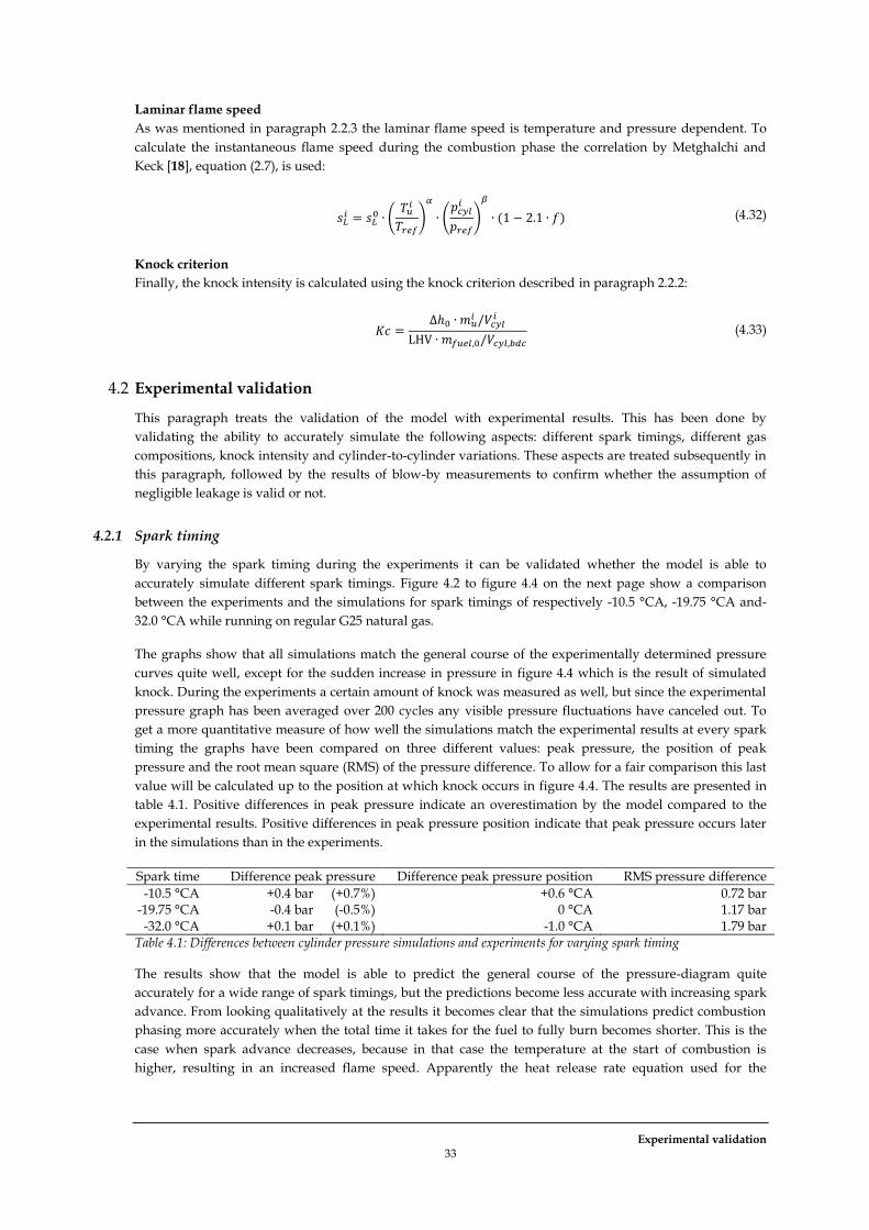
Experimental validation 33

Laminar flame speed

As was mentioned in paragraph 2.2.3 the laminar flame speed is temperature and pressure dependent. To

calculate the instantaneous flame speed during the combustion phase the correlation by Metghalchi and

Keck [18], equation (2.7), is used:

(4.32)

Knock criterion

Finally, the knock intensity is calculated using the knock criterion described in paragraph 2.2.2:

(4.33)

4.2 Experimental validation

This paragraph treats the validation of the model with experimental results. This has been done by

validating the ability to accurately simulate the following aspects: different spark timings, different gas

compositions, knock intensity and cylinder-to-cylinder variations. These aspects are treated subsequently in

this paragraph, followed by the results of blow-by measurements to confirm whether the assumption of

negligible leakage is valid or not.

4.2.1 Spark timing

By varying the spark timing during the experiments it can be validated whether the model is able to

accurately simulate different spark timings. Figure 4.2 to figure 4.4 on the next page show a comparison

between the experiments and the simulations for spark timings of respectively -10.5 °CA, -19.75 °CA and-

32.0 °CA while running on regular G25 natural gas.

The graphs show that all simulations match the general course of the experimentally determined pressure

curves quite well, except for the sudden increase in pressure in figure 4.4 which is the result of simulated

knock. During the experiments a certain amount of knock was measured as well, but since the experimental

pressure graph has been averaged over 200 cycles any visible pressure fluctuations have canceled out. To

get a more quantitative measure of how well the simulations match the experimental results at every spark

timing the graphs have been compared on three different values: peak pressure, the position of peak

pressure and the root mean square (RMS) of the pressure difference. To allow for a fair comparison this last

value will be calculated up to the position at which knock occurs in figure 4.4. The results are presented in

table 4.1. Positive differences in peak pressure indicate an overestimation by the model compared to the

experimental results. Positive differences in peak pressure position indicate that peak pressure occurs later

in the simulations than in the experiments.

Spark time Difference peak pressure Difference peak pressure position RMS pressure difference

-10.5 °CA +0.4 bar (+0.7%) +0.6 °CA 0.72 bar -19.75 °CA -0.4 bar (-0.5%) 0 °CA 1.17 bar -32.0 °CA +0.1 bar (+0.1%) -1.0 °CA 1.79 bar

Table 4.1: Differences between cylinder pressure simulations and experiments for varying spark timing

The results show that the model is able to predict the general course of the pressure-diagram quite

accurately for a wide range of spark timings, but the predictions become less accurate with increasing spark

advance. From looking qualitatively at the results it becomes clear that the simulations predict combustion

phasing more accurately when the total time it takes for the fuel to fully burn becomes shorter. This is the

case when spark advance decreases, because in that case the temperature at the start of combustion is

higher, resulting in an increased flame speed. Apparently the heat release rate equation used for the

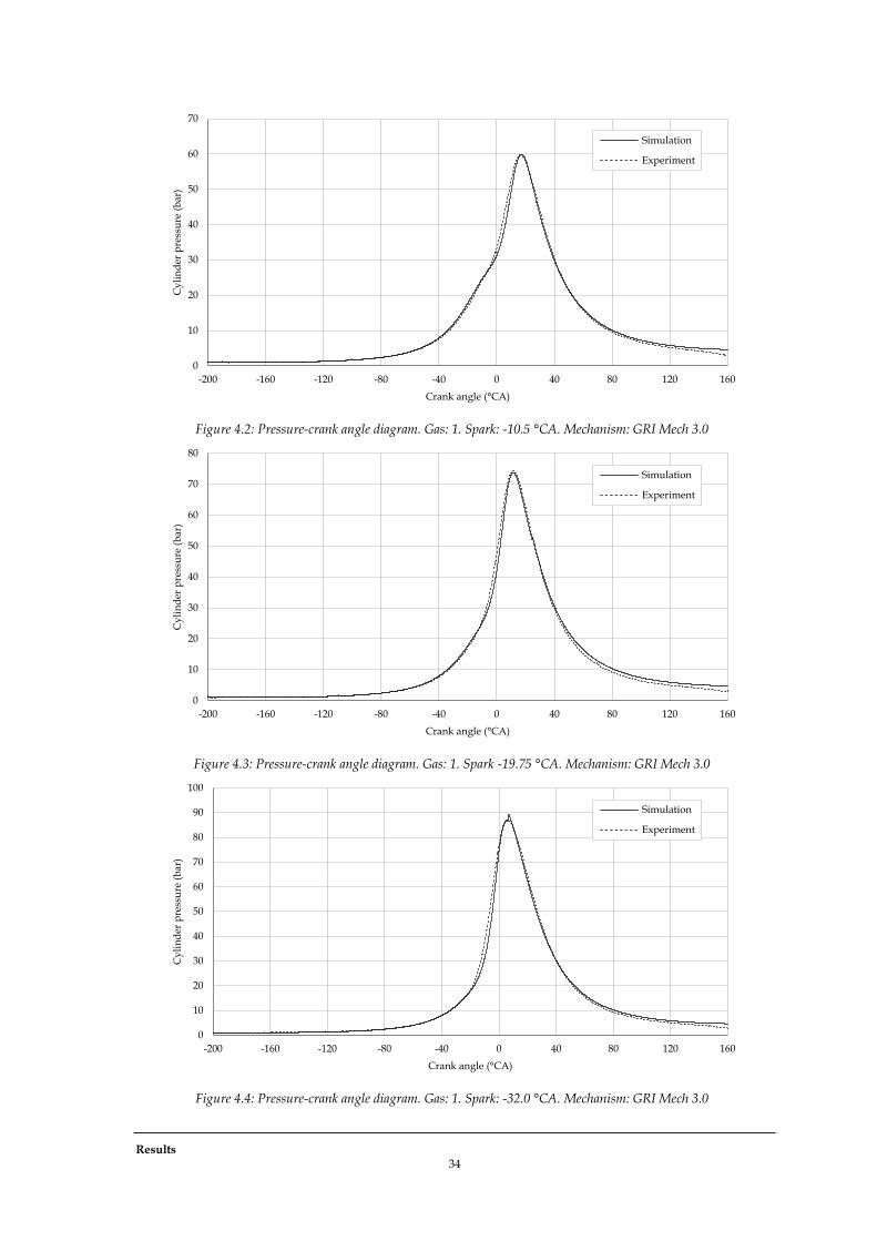
Results 34

Figure 4.2: Pressure-crank angle diagram. Gas: 1. Spark: -10.5 °CA. Mechanism: GRI Mech 3.0

Figure 4.3: Pressure-crank angle diagram. Gas: 1. Spark -19.75 °CA. Mechanism: GRI Mech 3.0

Figure 4.4: Pressure-crank angle diagram. Gas: 1. Spark: -32.0 °CA. Mechanism: GRI Mech 3.0

0

10

20

30

40

50

60

70

-200 -160 -120 -80 -40 0 40 80 120 160

Cy

lin

der

pre

ssu

re (

bar

)

Crank angle (°CA)

Simulation

Experiment

0

10

20

30

40

50

60

70

80

-200 -160 -120 -80 -40 0 40 80 120 160

Cy

lin

der

pre

ssu

re (

bar

)

Crank angle (°CA)

Simulation

Experiment

0

10

20

30

40

50

60

70

80

90

100

-200 -160 -120 -80 -40 0 40 80 120 160

Cy

lin

der

pre

ssu

re (

bar

)

Crank angle (°CA)

Simulation

Experiment

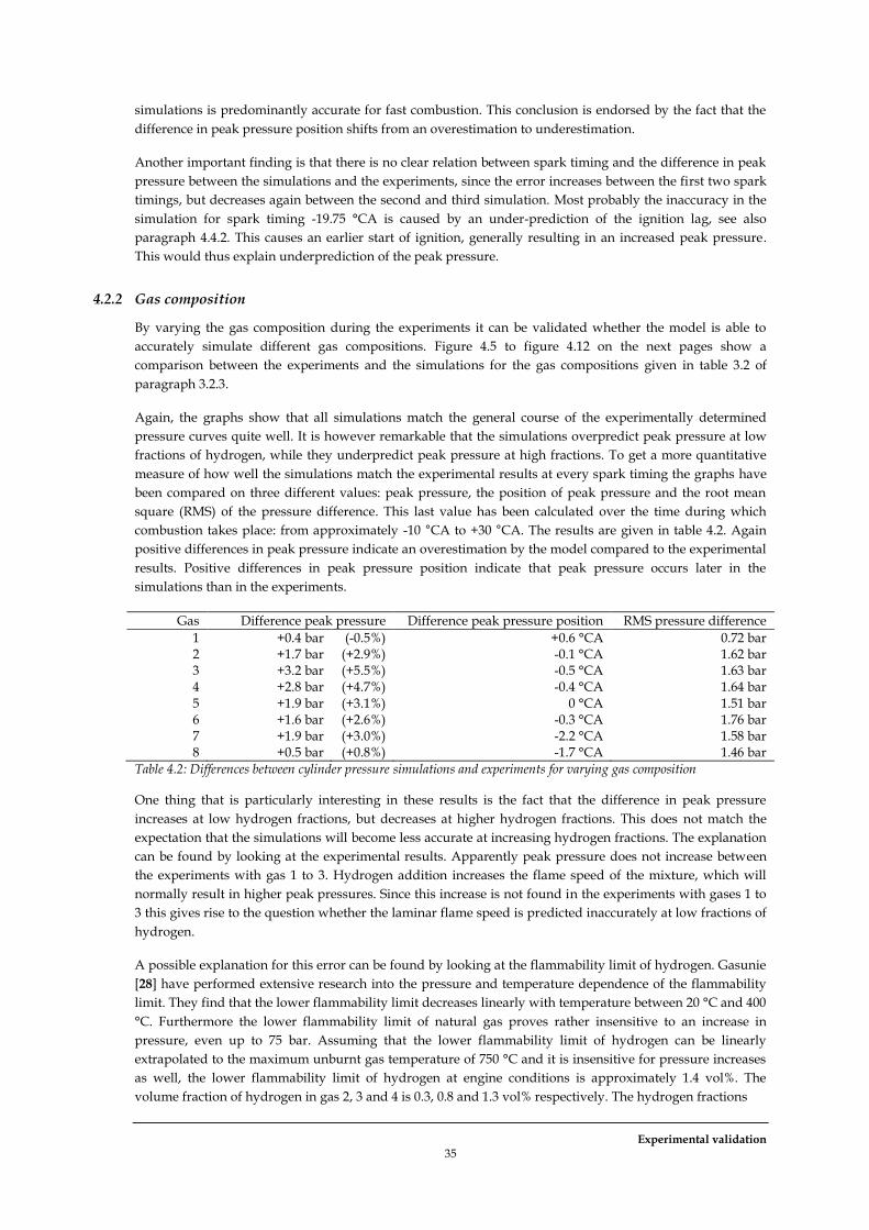
Experimental validation 35

simulations is predominantly accurate for fast combustion. This conclusion is endorsed by the fact that the

difference in peak pressure position shifts from an overestimation to underestimation.

Another important finding is that there is no clear relation between spark timing and the difference in peak

pressure between the simulations and the experiments, since the error increases between the first two spark

timings, but decreases again between the second and third simulation. Most probably the inaccuracy in the

simulation for spark timing -19.75 °CA is caused by an under-prediction of the ignition lag, see also

paragraph 4.4.2. This causes an earlier start of ignition, generally resulting in an increased peak pressure.

This would thus explain underprediction of the peak pressure.

4.2.2 Gas composition

By varying the gas composition during the experiments it can be validated whether the model is able to

accurately simulate different gas compositions. Figure 4.5 to figure 4.12 on the next pages show a

comparison between the experiments and the simulations for the gas compositions given in table 3.2 of

paragraph 3.2.3.

Again, the graphs show that all simulations match the general course of the experimentally determined

pressure curves quite well. It is however remarkable that the simulations overpredict peak pressure at low

fractions of hydrogen, while they underpredict peak pressure at high fractions. To get a more quantitative

measure of how well the simulations match the experimental results at every spark timing the graphs have

been compared on three different values: peak pressure, the position of peak pressure and the root mean

square (RMS) of the pressure difference. This last value has been calculated over the time during which

combustion takes place: from approximately -10 °CA to +30 °CA. The results are given in table 4.2. Again

positive differences in peak pressure indicate an overestimation by the model compared to the experimental

results. Positive differences in peak pressure position indicate that peak pressure occurs later in the

simulations than in the experiments.

Gas Difference peak pressure Difference peak pressure position RMS pressure difference

1 +0.4 bar (-0.5%) +0.6 °CA 0.72 bar 2 +1.7 bar (+2.9%) -0.1 °CA 1.62 bar 3 +3.2 bar (+5.5%) -0.5 °CA 1.63 bar 4 +2.8 bar (+4.7%) -0.4 °CA 1.64 bar 5 +1.9 bar (+3.1%) 0 °CA 1.51 bar 6 +1.6 bar (+2.6%) -0.3 °CA 1.76 bar 7 +1.9 bar (+3.0%) -2.2 °CA 1.58 bar 8 +0.5 bar (+0.8%) -1.7 °CA 1.46 bar

Table 4.2: Differences between cylinder pressure simulations and experiments for varying gas composition

One thing that is particularly interesting in these results is the fact that the difference in peak pressure

increases at low hydrogen fractions, but decreases at higher hydrogen fractions. This does not match the

expectation that the simulations will become less accurate at increasing hydrogen fractions. The explanation

can be found by looking at the experimental results. Apparently peak pressure does not increase between

the experiments with gas 1 to 3. Hydrogen addition increases the flame speed of the mixture, which will

normally result in higher peak pressures. Since this increase is not found in the experiments with gases 1 to

3 this gives rise to the question whether the laminar flame speed is predicted inaccurately at low fractions of

hydrogen.

A possible explanation for this error can be found by looking at the flammability limit of hydrogen. Gasunie

[28] have performed extensive research into the pressure and temperature dependence of the flammability

limit. They find that the lower flammability limit decreases linearly with temperature between 20 °C and 400

°C. Furthermore the lower flammability limit of natural gas proves rather insensitive to an increase in

pressure, even up to 75 bar. Assuming that the lower flammability limit of hydrogen can be linearly

extrapolated to the maximum unburnt gas temperature of 750 °C and it is insensitive for pressure increases

as well, the lower flammability limit of hydrogen at engine conditions is approximately 1.4 vol%. The

volume fraction of hydrogen in gas 2, 3 and 4 is 0.3, 0.8 and 1.3 vol% respectively. The hydrogen fractions

Results 36

Figure 4.5: Pressure-crank angle diagram. Gas: 1. Spark: -10.5 °CA. Mechanism: GRI Mech 3.0

Figure 4.6: Pressure-crank angle diagram. Gas: 2. Spark -10.0 °CA. Mechanism: GRI Mech 3.0

Figure 4.7: Pressure-crank angle diagram. Gas: 3. Spark: -10.0 °CA. Mechanism: GRI Mech 3.0

0

10

20

30

40

50

60

70

-200 -160 -120 -80 -40 0 40 80 120 160

Cy

lin

der

pre

ssu

re (

bar

)

Crank angle (°CA)

Simulation

Experiment

0

10

20

30

40

50

60

70

-200 -160 -120 -80 -40 0 40 80 120 160

Cy

lin

der

pre

ssu

re (

bar

)

Crank angle (°CA)

Simulation

Experiment

0

10

20

30

40

50

60

70

-200 -160 -120 -80 -40 0 40 80 120 160

Cy

lin

der

pre

ssu

re (

bar

)

Crank angle (°CA)

Simulation

Experiment

Experimental validation 37

Figure 4.8: Pressure-crank angle diagram. Gas: 4. Spark: -9.75 °CA. Mechanism: GRI Mech 3.0

Figure 4.9: Pressure-crank angle diagram. Gas: 5. Spark -9.75 °CA. Mechanism: GRI Mech 3.0

Figure 4.10: Pressure-crank angle diagram. Gas: 6. Spark: -10.0 °CA. Mechanism: GRI Mech 3.0

0

10

20

30

40

50

60

70

-200 -160 -120 -80 -40 0 40 80 120 160

Cy

lin

der

pre

ssu

re (

bar

)

Crank angle (°CA)

Simulation

Experiment

0

10

20

30

40

50

60

70

-200 -160 -120 -80 -40 0 40 80 120 160

Cy

lin

der

pre

ssu

re (

bar

)

Crank angle (°CA)

Simulation

Experiment

0

10

20

30

40

50

60

70

-200 -160 -120 -80 -40 0 40 80 120 160

Cy

lin

der

pre

ssu

re (

bar

)

Crank angle (°CA)

Simulation

Experiment

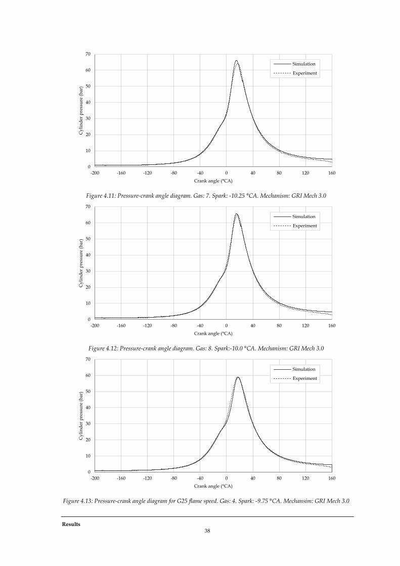
Results 38

Figure 4.11: Pressure-crank angle diagram. Gas: 7. Spark: -10.25 °CA. Mechanism: GRI Mech 3.0

Figure 4.12: Pressure-crank angle diagram. Gas: 8. Spark:-10.0 °CA. Mechanism: GRI Mech 3.0

Figure 4.13: Pressure-crank angle diagram for G25 flame speed. Gas: 4. Spark: -9.75 °CA. Mechansim: GRI Mech 3.0

0

10

20

30

40

50

60

70

-200 -160 -120 -80 -40 0 40 80 120 160

Cy

lin

der

pre

ssu

re (

bar

)

Crank angle (°CA)

Simulation

Experiment

0

10

20

30

40

50

60

70

-200 -160 -120 -80 -40 0 40 80 120 160

Cy

lin

der

pre

ssu

re (

bar

)

Crank angle (°CA)

Simulation

Experiment

0

10

20

30

40

50

60

70

-200 -160 -120 -80 -40 0 40 80 120 160

Cy

lin

der

pre

ssu

re (

bar

)

Crank angle (°CA)

Simulation

Experiment

Experimental validation 39

in these experiments would therefore be too small to allow flame propagation, thus the flame propagates

with the flame speed of natural gas. This would explain why the experiments with these gases show no

increase in peak pressure. To check this assumption the simulation with gas 4 has been performed again

with the flame speed of gas 1. The resulting pressure-crank angle diagram can be found in figure 4.13. A

comparison to the first simulation (figure 4.8) shows that the new simulation indeed fits the experimental

results much better, therefore supporting the explanation involving the lower flammability limit.

Another interesting finding is the fact that the difference in peak pressure position is remarkably larger for

the gases with the highest hydrogen fractions (gas 7 and 8), while the differences between gas 2 to 6 are

significantly smaller. Since the flame speed predictions seem to become more accurate at increasing

hydrogen fraction, it is unlikely that this error has the same cause as the error in peak pressure. One

plausible explanation could be the fact that the knock limit spark time for both gas 7 and 8 has been

determined at -12 °CA, which means that at these experimental conditions (spark at -10 °CA) there is

already a considerable knock intensity. This could be the reason why the shape of the pressure curves of

these experiments show more deviation from the pressure curves predicted by the simulations.

4.2.3 Knock criterion and knock limit spark time

During the experiments the knock limit spark time (KLST) has been determined for all test gases using the

Siemens-VDO method (see paragraph 2.3.1). This method is based on the amplitude of the pressure

oscillations in the cylinder resulting from energy released by the unburnt gases. The knock criterion which

results from the simulations is also based on the energy content of the unburnt gases, which makes it

reasonable to assume there is a relation between the experimentally determined KLST of a gas and the

corresponding knock factor resulting from the simulation. Table 4.3 shows the experimentally determined

knock limit spark time for the different test gases, while figure 4.14 shows the corresponding values of the

knock criterion. The results of this graph have been obtained by running simulations for every test gas at

their respective KLST. The simulations have been performed using three different chemical mechanisms to

investigate the capability of each mechanism to predict knock occurrence.

Figure 4.14 reveals that both the nC5_50 and C3_41 chemical mechanism give fairly constant values for the

knock criterion at KLST, with slight deviations for gas 2 and 3. For GRI Mech 3.0 there is no clear relation

between the different values of the knock criterion.

Gas 1 2 3 4 5 6 7 8 KLST * -33 °CA -25 °CA -20 °CA -20 °CA -17 °CA -12 °CA -12 °CA Table 4.3: Experimentally determined knock limit spark time for all test gases (*KLST could not be determined)

Figure 4.14: Knock criterion at knock limit spark time for different test gases and different chemical mechanisms.

0.4

0.6

0.8

1

1.2

1.4

1.6

1.8

2

2 3 4 5 6 7 8

Kn

ock

cri

teri

on

(-)

Test gas

nC5_50

C3_41

GRI Mech 3.0

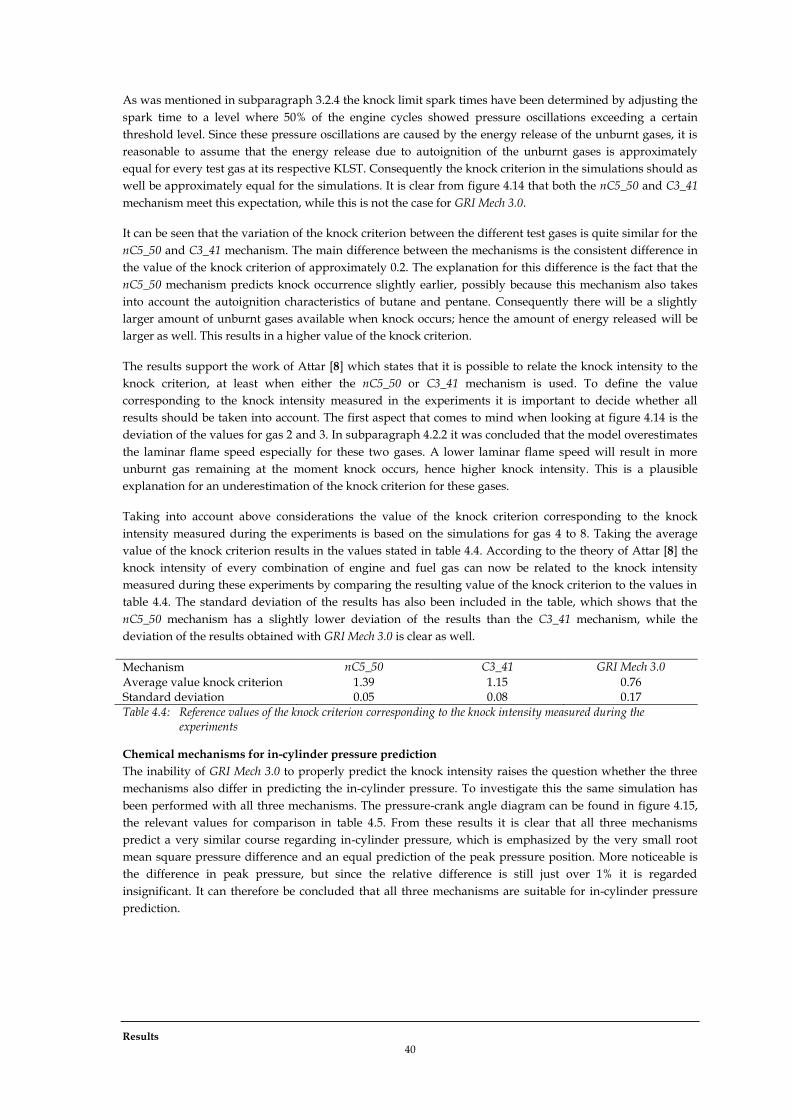
Results 40

As was mentioned in subparagraph 3.2.4 the knock limit spark times have been determined by adjusting the

spark time to a level where 50% of the engine cycles showed pressure oscillations exceeding a certain

threshold level. Since these pressure oscillations are caused by the energy release of the unburnt gases, it is

reasonable to assume that the energy release due to autoignition of the unburnt gases is approximately

equal for every test gas at its respective KLST. Consequently the knock criterion in the simulations should as

well be approximately equal for the simulations. It is clear from figure 4.14 that both the nC5_50 and C3_41

mechanism meet this expectation, while this is not the case for GRI Mech 3.0.

It can be seen that the variation of the knock criterion between the different test gases is quite similar for the

nC5_50 and C3_41 mechanism. The main difference between the mechanisms is the consistent difference in

the value of the knock criterion of approximately 0.2. The explanation for this difference is the fact that the

nC5_50 mechanism predicts knock occurrence slightly earlier, possibly because this mechanism also takes

into account the autoignition characteristics of butane and pentane. Consequently there will be a slightly

larger amount of unburnt gases available when knock occurs; hence the amount of energy released will be

larger as well. This results in a higher value of the knock criterion.

The results support the work of Attar [8] which states that it is possible to relate the knock intensity to the

knock criterion, at least when either the nC5_50 or C3_41 mechanism is used. To define the value

corresponding to the knock intensity measured in the experiments it is important to decide whether all

results should be taken into account. The first aspect that comes to mind when looking at figure 4.14 is the

deviation of the values for gas 2 and 3. In subparagraph 4.2.2 it was concluded that the model overestimates

the laminar flame speed especially for these two gases. A lower laminar flame speed will result in more

unburnt gas remaining at the moment knock occurs, hence higher knock intensity. This is a plausible

explanation for an underestimation of the knock criterion for these gases.

Taking into account above considerations the value of the knock criterion corresponding to the knock

intensity measured during the experiments is based on the simulations for gas 4 to 8. Taking the average

value of the knock criterion results in the values stated in table 4.4. According to the theory of Attar [8] the

knock intensity of every combination of engine and fuel gas can now be related to the knock intensity

measured during these experiments by comparing the resulting value of the knock criterion to the values in

table 4.4. The standard deviation of the results has also been included in the table, which shows that the

nC5_50 mechanism has a slightly lower deviation of the results than the C3_41 mechanism, while the

deviation of the results obtained with GRI Mech 3.0 is clear as well.

Mechanism nC5_50 C3_41 GRI Mech 3.0

Average value knock criterion 1.39 1.15 0.76 Standard deviation 0.05 0.08 0.17 Table 4.4: Reference values of the knock criterion corresponding to the knock intensity measured during the experiments

Chemical mechanisms for in-cylinder pressure prediction

The inability of GRI Mech 3.0 to properly predict the knock intensity raises the question whether the three

mechanisms also differ in predicting the in-cylinder pressure. To investigate this the same simulation has

been performed with all three mechanisms. The pressure-crank angle diagram can be found in figure 4.15,

the relevant values for comparison in table 4.5. From these results it is clear that all three mechanisms

predict a very similar course regarding in-cylinder pressure, which is emphasized by the very small root

mean square pressure difference and an equal prediction of the peak pressure position. More noticeable is

the difference in peak pressure, but since the relative difference is still just over 1% it is regarded

insignificant. It can therefore be concluded that all three mechanisms are suitable for in-cylinder pressure

prediction.

Experimental validation 41

Figure 4.15: Pressure-crank angle diagram for different chemical mechanisms. Gas: 1. Spark: -19.75°

Mechanism Difference peak pressure Difference peak pressure position RMS pressure difference C3_41 +0.84 bar (+1.1%) 0 °CA 0.33

nC5_50 +0.81 bar (+1.1%) 0 °CA 0.37 Table 4.5: Differences between simulations using different chemical mechanisms with respect to the simulation using GRI Mech 3.0

4.2.4 Cylinder-to-cylinder variations

Figure 4.16 shows the pressure curves measured in all eight cylinders of the test engine. It immediately

becomes clear that there are significant cylinder-to-cylinder variations between the respective pressure

curves. More importantly, there seems to be a significant deviation between the cylinders in the left and

right bank (cylinders 1 to 4 and 5 to 8 respectively) of the engine. A possible explanation could be an

unequal distribution of fresh mixture over the cylinders. Furthermore, close inspection of the heat release

rate (figure 4.17) learns that combustion duration is shorter in the right bank, which could also explain the

increased peak pressures in these cylinders.

Inspection of the experimental results learns that the average combustion duration during normal operation

(gas 1, spark -20 °CA) is 36 °CA for cylinder 8 and 46 °CA for cylinder 1 (based on 90% fuel burnt). This

indicates that the flame speed in cylinder 8 should be about 28% higher compared to cylinder 1. The

increased flame speed in the cylinders of the right bank could be caused by two phenomena:

Higher mixture temperature

Enhanced mixing of fuel and air

Since neither one of these two aspects nor the mixture distribution could be measured during the

experiments, a large number of simulations has been performed to see what combination of variables gives

the best fit for cylinder 1 and cylinder 8. The results can be found in figure 4.18. The difference between the

simulations is in the turbulence factor C of the heat release correlation (equation (4.20)) only. This means

that the mixture distribution and the initial mixture temperature are equal for all cylinders in the

simulations.

The difference in turbulence factor between the cylinders is 23%, which corresponds well to the difference in

flame speed mentioned before. Because all the cylinders in the right bank of the engine show an increased

peak pressure, a reasonable assumption is that the difference in turbulence level is caused in the manifold

and not in the cylinders itself.

0

10

20

30

40

50

60

70

80

-200 -160 -120 -80 -40 0 40 80 120 160

Cy

lin

der

pre

ssu

re (

bar

)

Crank angle (°CA)

GRI Mech 3.0

C3_41 mech

nC5_50 mech

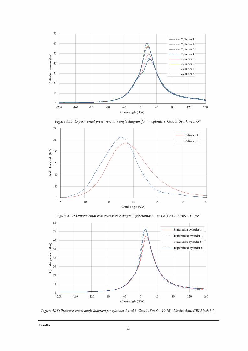
Results 42

Figure 4.16: Experimental pressure-crank angle diagram for all cylinders. Gas: 1. Spark: -10.75°

Figure 4.17: Experimental heat release rate diagram for cylinder 1 and 8. Gas 1. Spark: -19.75°

Figure 4.18: Pressure-crank angle diagram for cylinder 1 and 8. Gas: 1. Spark: -19.75°. Mechanism: GRI Mech 3.0

0

10

20

30

40

50

60

70

-200 -160 -120 -80 -40 0 40 80 120 160

Cy

lin

der

pre

ssu

re (

bar

)

Crank angle (°CA)

Cylinder 1

Cylinder 2

Cylinder 3

Cylinder 4

Cylinder 5

Cylinder 6

Cylinder 7

Cylinder 8

0

40

80

120

160

200

240

-20 -10 0 10 20 30 40

Hea

t re

leas

e ra

te (

J/°)

Crank angle (°CA)

Cylinder 1

Cylinder 8

0

10

20

30

40

50

60

70

80

-200 -160 -120 -80 -40 0 40 80 120 160

Cy

lin

der

pre

ssu

re (

bar

)

Crank angle (°CA)

Simulation cylinder 1

Experiment cylinder 1

Simulation cylinder 8

Experiment cylinder 8

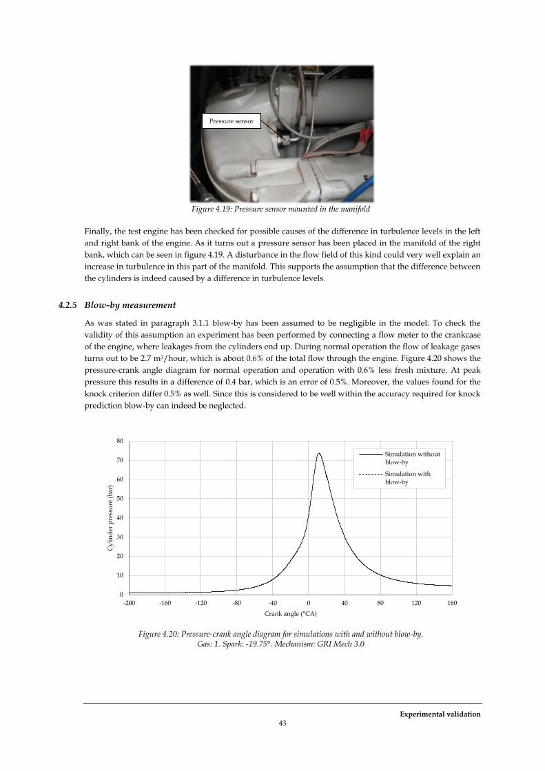
Experimental validation 43

Figure 4.19: Pressure sensor mounted in the manifold

Finally, the test engine has been checked for possible causes of the difference in turbulence levels in the left

and right bank of the engine. As it turns out a pressure sensor has been placed in the manifold of the right

bank, which can be seen in figure 4.19. A disturbance in the flow field of this kind could very well explain an

increase in turbulence in this part of the manifold. This supports the assumption that the difference between

the cylinders is indeed caused by a difference in turbulence levels.

4.2.5 Blow-by measurement

As was stated in paragraph 3.1.1 blow-by has been assumed to be negligible in the model. To check the

validity of this assumption an experiment has been performed by connecting a flow meter to the crankcase

of the engine, where leakages from the cylinders end up. During normal operation the flow of leakage gases

turns out to be 2.7 m3/hour, which is about 0.6% of the total flow through the engine. Figure 4.20 shows the

pressure-crank angle diagram for normal operation and operation with 0.6% less fresh mixture. At peak

pressure this results in a difference of 0.4 bar, which is an error of 0.5%. Moreover, the values found for the

knock criterion differ 0.5% as well. Since this is considered to be well within the accuracy required for knock

prediction blow-by can indeed be neglected.

Figure 4.20: Pressure-crank angle diagram for simulations with and without blow-by.

Gas: 1. Spark: -19.75°. Mechanism: GRI Mech 3.0

0

10

20

30

40

50

60

70

80

-200 -160 -120 -80 -40 0 40 80 120 160

Cy

lin

der

pre

ssu

re (

bar

)

Crank angle (°CA)

Simulation without blow-by

Simulation with blow-by

Pressure sensor

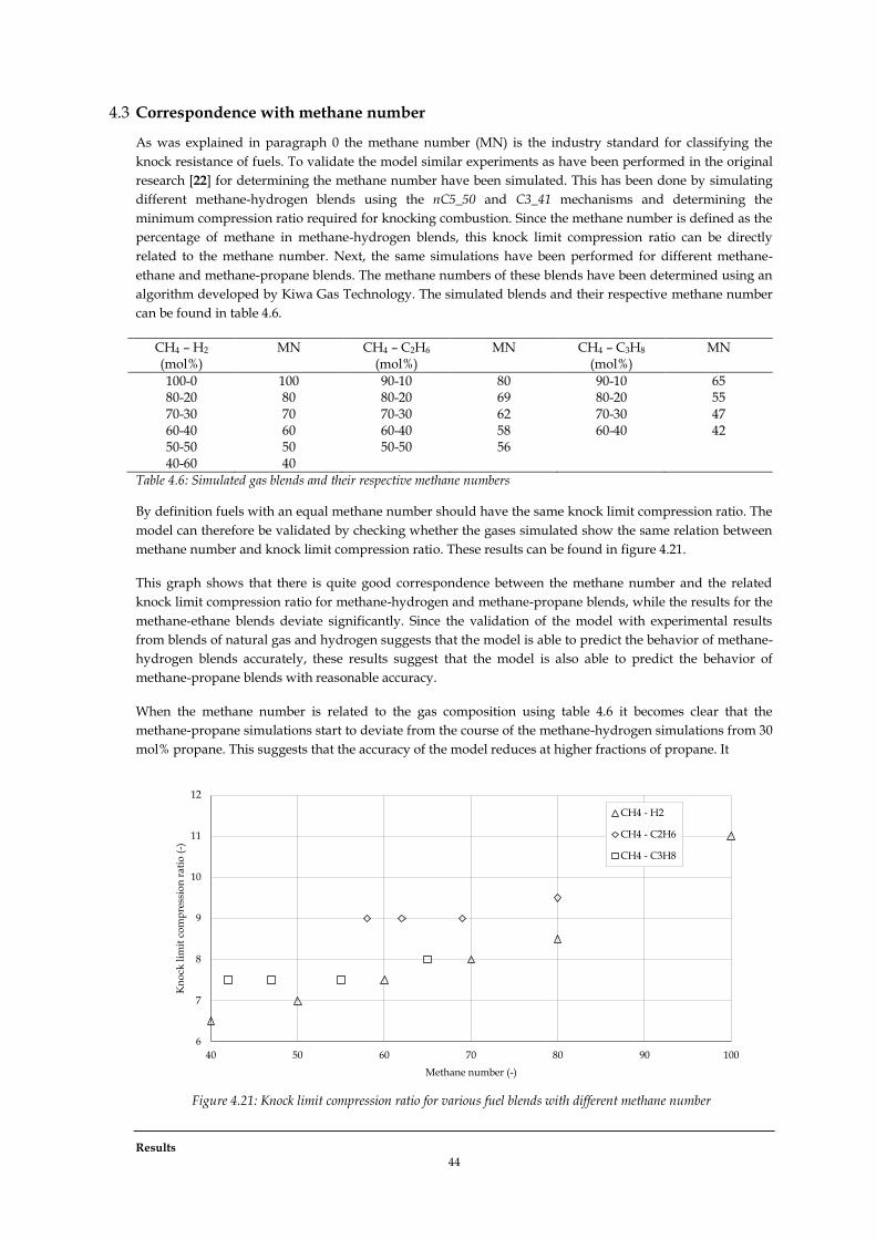
Results 44

4.3 Correspondence with methane number

As was explained in paragraph 0 the methane number (MN) is the industry standard for classifying the

knock resistance of fuels. To validate the model similar experiments as have been performed in the original

research [22] for determining the methane number have been simulated. This has been done by simulating

different methane-hydrogen blends using the nC5_50 and C3_41 mechanisms and determining the

minimum compression ratio required for knocking combustion. Since the methane number is defined as the

percentage of methane in methane-hydrogen blends, this knock limit compression ratio can be directly

related to the methane number. Next, the same simulations have been performed for different methane-

ethane and methane-propane blends. The methane numbers of these blends have been determined using an

algorithm developed by Kiwa Gas Technology. The simulated blends and their respective methane number

can be found in table 4.6.

CH4 – H2 (mol%)

MN CH4 – C2H6 (mol%)

MN CH4 – C3H8 (mol%)

MN

100-0 100 90-10 80 90-10 65 80-20 80 80-20 69 80-20 55 70-30 70 70-30 62 70-30 47 60-40 60 60-40 58 60-40 42 50-50 50 50-50 56 40-60 40

Table 4.6: Simulated gas blends and their respective methane numbers

By definition fuels with an equal methane number should have the same knock limit compression ratio. The

model can therefore be validated by checking whether the gases simulated show the same relation between

methane number and knock limit compression ratio. These results can be found in figure 4.21.

This graph shows that there is quite good correspondence between the methane number and the related

knock limit compression ratio for methane-hydrogen and methane-propane blends, while the results for the

methane-ethane blends deviate significantly. Since the validation of the model with experimental results

from blends of natural gas and hydrogen suggests that the model is able to predict the behavior of methane-

hydrogen blends accurately, these results suggest that the model is also able to predict the behavior of

methane-propane blends with reasonable accuracy.

When the methane number is related to the gas composition using table 4.6 it becomes clear that the

methane-propane simulations start to deviate from the course of the methane-hydrogen simulations from 30

mol% propane. This suggests that the accuracy of the model reduces at higher fractions of propane. It

Figure 4.21: Knock limit compression ratio for various fuel blends with different methane number

6

7

8

9

10

11

12

40 50 60 70 80 90 100

Kn

ock

lim

it c

om

pre

ssio

n r

atio

(-)

Methane number (-)

CH4 - H2

CH4 - C2H6

CH4 - C3H8

Correspondence with methane number 45

should however be noted that this cannot be said with certainty, because the model has only been

experimentally validated with hydrogen blends up to 27 mol%. Since the methane number of a 30 mol%

propane blend corresponds to that of a hydrogen blend of 53 mol%, it is also uncertain if the corresponding

methane-hydrogen simulation is accurate. However, the methane-hydrogen simulations show a more

plausible course than the methane-propane simulations, since the knock limit compression ratio of methane-

propane blends seems to stabilize at a constant value while a decreasing value is expected. Therefore it is

plausible to assume the model becomes less accurate for gases with propane fractions higher than 20 mol%.

The other remarkable result is the fact that the methane-ethane simulations deviate significantly from the

methane-hydrogen simulations for every fraction of ethane. This raises the question what particular aspect

of the simulations causes this difference. The particular simulations differ in only two input variables: gas

composition and laminar flame speed. Furthermore the accuracy of the methane number algorithm is also

unknown. The accuracy of the laminar flame speed and methane number have been cross checked with

other references, see table 4.7 and table 4.8.

CH4 – C2H6 (mol%) 90-10 80-20 70-30 60-40 50-50 Methane number (Kiwa method)

80 69 62 58 56

Methane number [21] 80 69 62 58 55

Table 4.7: Methane number for different methane-ethane blends according to Kiwa method and Klimstra et al. [21]

CH4 – C2H6 (mol%) 90-10 80-20 70-30 60-40 50-50 Laminar flame speed (m/s) (Cantera)

0.389 0.394 0.399 0.404 0.408

Laminar flame speed (m/s) [29]

0.386 0.397 0.405 * *

Table 4.8: Laminar flame speed for different methane-ethane blends according to numerical calculations and Dirrenberger et al. [29] (*flame speed was not determined)

Table 4.7 shows that the methane numbers determined using the Kiwa method correspond nearly perfectly

to the ones from Klimstra et al. [21], while table 4.8 shows that there are only minor differences between the

numerically calculated flame speed using Cantera and the values found by Dirrenberger et al. [29]. The

similarities suggest that the deviations of the methane-ethane simulations are not the result of erroneous

predictions of either the methane number or the laminar flame speed. From this observation can be

concluded that the deviations must be caused by the only variable left: gas composition, hence by

irregularities in the chemical mechanism.

The reaction path of a methane-ethane simulation and a methane-propane simulation has been investigated

in more detail to find any effects supporting the former conclusion. To this end the creation and destruction

rates of particular species have been investigated for both simulations. The focus of the analysis has been on

the species involved in the important knock reactions treated in paragraph 2.4: equations (2.13) - (2.17). The

most remarkable difference between the ethane and propane simulations is related to the results found in

figure 4.22 to figure 4.25, showing the destruction and creation rate of four species in the unburnt gas during

both simulations.

The graphs show the first phase of autoignition and are related to the following reaction:

(4.34)

If the chemical mechanism follows the reaction path as was described in paragraph 2.4, above reaction

should be incorporated. The reaction describes how for every mole of reactant R‟OOH one mole of OH will

result. Figure 4.24 and figure 4.25 show that in the methane-propane simulation the destruction rate of

C3H6OOH is nearly equal to the creation rate of OH, indicating that above reaction is indeed occurring

during the start of autoignition of the unburnt gas. Figure 4.22 and figure 4.23 however indicate that there is

no such relation between C2H4OOH and OH in the methane-ethane simulations. Apparently other reactions

resulting in the formation of OH are taking place. This means that the reaction path described in paragraph

Results 46

2.4 is not the principal reaction path for autoignition in the methane-ethane simulations. Possibly the

reaction path actually followed during the simulations is that of regular combustion, which requires higher

temperatures compared to knocking combustion. This would hence require a higher compression ratio and

is thus a plausible explanation why these simulations do not show the expected relation between methane

number and knock limit compression ratio.

Figure 4.22: C2H4OOH destruction rate in methane-ethane simulation

Figure 4.23: OH creation rate in methane-ethane simulation

Figure 4.24: C3H6OOH destruction rate in methane-propane simulation

Figure 4.25: OH creation rate in methane-propane simulation

0.00E+00

5.00E-04

1.00E-03

1.50E-03

2.00E-03

2.50E-03

3.00E-03

-16 -12 -8 -4 0 4 8

Des

tru

ctio

n r

ate

(km

ol/

m3/

s)

Crank angle (°CA)

0.00E+00

2.50E-02

5.00E-02

7.50E-02

1.00E-01

1.25E-01

1.50E-01

1.75E-01

2.00E-01

-16 -12 -8 -4 0 4 8 C

reat

ion

rat

e (k

mo

l/m

3/

s)

Crank angle (°CA)

0.00E+00

2.00E-02

4.00E-02

6.00E-02

8.00E-02

1.00E-01

1.20E-01

-16 -12 -8 -4 0 4 8

Des

tru

ctio

n r

ate

(km

ol/

m3/

s)

Crank angle (°CA)

0.00E+00

2.00E-02

4.00E-02

6.00E-02

8.00E-02

1.00E-01

1.20E-01

-16 -12 -8 -4 0 4 8

Cre

atio

n r

ate

(km

ol/

m3/

s)

Crank angle (°CA)

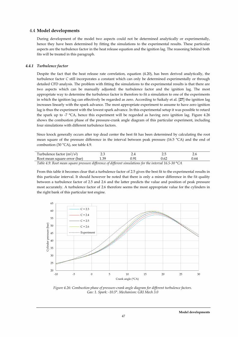
Model developments 47

4.4 Model developments

During development of the model two aspects could not be determined analytically or experimentally,

hence they have been determined by fitting the simulations to the experimental results. These particular

aspects are the turbulence factor in the heat release equation and the ignition lag. The reasoning behind both

fits will be treated in this paragraph.

4.4.1 Turbulence factor

Despite the fact that the heat release rate correlation, equation (4.20), has been derived analytically, the

turbulence factor C still incorporates a constant which can only be determined experimentally or through

detailed CFD analysis. The problem with fitting the simulations to the experimental results is that there are

two aspects which can be manually adjusted: the turbulence factor and the ignition lag. The most

appropriate way to determine the turbulence factor is therefore to fit a simulation to one of the experiments

in which the ignition lag can effectively be regarded as zero. According to Saikaly et al. [27] the ignition lag

increases linearly with the spark advance. The most appropriate experiment to assume to have zero ignition

lag is thus the experiment with the lowest spark advance. In this experimental setup it was possible to retard

the spark up to -7 °CA, hence this experiment will be regarded as having zero ignition lag. Figure 4.26

shows the combustion phase of the pressure-crank angle diagram of this particular experiment, including

four simulations with different turbulence factors.

Since knock generally occurs after top dead center the best fit has been determined by calculating the root

mean square of the pressure difference in the interval between peak pressure (16.5 °CA) and the end of

combustion (30 °CA), see table 4.9.

Turbulence factor (m2/s2) 2.3 2.4 2.5 2.6 Root mean square error (bar) 1.39 0.91 0.62 0.64 Table 4.9: Root mean square pressure difference of different simulations for the interval 16.5-30 °CA

From this table it becomes clear that a turbulence factor of 2.5 gives the best fit to the experimental results in

this particular interval. It should however be noted that there is only a minor difference in the fit quality

between a turbulence factor of 2.5 and 2.6 and the latter predicts the value and position of peak pressure

most accurately. A turbulence factor of 2.6 therefore seems the most appropriate value for the cylinders in

the right bank of this particular test engine.

Figure 4.26: Combustion phase of pressure-crank angle diagram for different turbulence factors.

Gas: 1. Spark: -10.5°. Mechanism: GRI Mech 3.0

20

25

30

35

40

45

50

55

60

65

-10 -5 0 5 10 15 20 25 30

Cy

lin

der

pre

ssu

re (

bar

)

Crank angle (°CA)

C = 2.3

C = 2.4

C = 2.5

C = 2.6

Experiment

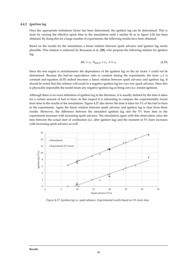
Results 48

4.4.2 Ignition lag

Once the appropriate turbulence factor has been determined, the ignition lag can be determined. This is

done by varying the effective spark time in the simulations until a similar fit as in figure 4.26 has been

obtained. By doing this for a large number of experiments, the following results have been obtained:

Based on the results for the simulations a linear relation between spark advance and ignition lag seems

plausible. This relation is endorsed by Rousseau et al. [30], who propose the following relation for ignition

lag:

(4.35)

Since the test engine is stoichiometric the dependence of the ignition lag on the air factor λ could not be

determined. Because the fuel-air equivalence ratio is constant during the experiments, the term c2∙λ is

constant and equation (4.35) indeed becomes a linear relation between spark advance and ignition lag. It

should be noted that this relation will result in a negative ignition lag for very low spark advance. Since this

is physically impossible the model treats any negative ignition lag as being zero (i.e. instant ignition).

Although there is no exact definition of ignition lag in the literature, it is usually defined by the time it takes

for a certain amount of fuel to burn. In this respect it is interesting to compare the experimentally found

burn time to the results of the simulations. Figure 4.27 also shows the time it takes for 5% of the fuel to burn

in the experiments. Again the linear relation between spark advance and ignition lag is clear from these

results. Moreover, the difference between the simulated ignition lag and the 5% burn time in the

experiments increases with increasing spark advance. The simulations agree with this observation, since the

time between the actual start of combustion (i.e. after ignition lag) and the moment of 5% burn increases

with increasing spark advance as well.

Figure 4.27: Ignition lag vs. spark advance. Experimental results based on 5% burn time.

0

2

4

6

8

10

12

14

16

0 5 10 15 20 25 30 35

Ign

itio

n l

ag (

°CA

)

Spark advance (°CA)

Simulations

Experiments (5% burn)

Sensitivity analysis 49

4.5 Sensitivity analysis

To investigate if the model is particularly sensitive to changes in certain parameters a sensitivity analysis has

been performed. To this end the test engine has been simulated running on regular natural gas and spark

advance at -30 °CA, while subsequently varying every input parameter and checking the resulting knock

intensity.

4.5.1 Engine parameters

A sensitivity analysis has been performed on the different engine parameters in the model by running

analyses with a 20% decrease and a 20% increase in the particular parameter. The results can be found in

table 4.10.

Bore Stroke Compression ratio

Connecting rod length

Engine speed Wall temperature

-20% +2% -2% -46% -1% +24% ±0% +20% +3% ±0% +129% -3% -19% ±0%

Table 4.10: Sensitivity of the knock intensity for a ±20% deviation of different engine parameters

Table 4.10 gives clear examples for why it is difficult to predict the change in knock intensity based on a

change in parameters. For example: both an increase and decrease of the bore result in an increased knock

intensity. In this case this is caused by an interaction between the unburnt gas mass, cylinder volume at the

moment of knock and cylinder volume at bottom dead center, which are all influenced by a change in bore.

More importantly, from table 4.10 can be concluded that the model is rather insensitive to changes in most

parameters, except for compression ratio and engine speed. In this respect it is interesting to estimate with

what accuracy the different parameters can be determined. These estimates can be found in table 4.11.

Bore Stroke Compression ratio

Connecting rod length

Engine speed Wall temperature

Uncertainty <1% <1% <3% <1% <1% <20%

Table 4.11: Estimated uncertainty of different engine parameters

Engine dimensions like bore, stroke and connecting rod length are quite easily measured and there are

hardly any restrictions for accurate measurements, so deviations of more than 1% are not expected in these

parameters. Compression ratio depends on several dimensions and may also be more difficult to determine

because of complicated combustion chamber geometries, the uncertainty is therefore somewhat higher. In

CHP applications the engine speed is known very accurately because it is directly related to the output

frequency of the alternating current, the expected deviation is therefore less than 1%. Wall temperature is

highly uncertain, because it is hard to measure directly, but the temperature of the cooling water gives a

reasonable estimation. The expected deviation of this parameter is however quite high.

By combining the expected deviation of the parameters with their respective sensitivity factors it can be

concluded that despite the relatively high sensitivity of the model for variations in engine speed, this should

not pose a problem because of the high accuracy with which this parameter can be determined. Additional

attention should however be paid to accurate determination of the compression ratio, because even the

small uncertainty might have a huge influence on the knock intensity. The sensitivity of this parameter has

therefore been investigated for smaller deviations. The results can be found in figure 4.28.

From figure 4.28 can be concluded that the sensitivity increases for increasing positive deviations of the

compression ratio, while it decreases for increasing negative deviations. In the latter case there is however

the risk that no knock is simulated. Although the sensitivity is lower at lower deviations, it is still over 10%

at the maximum uncertainty of 3%. It can therefore be concluded that special attention should indeed be

paid to determining the compression ratio accurately.

Results 50

Figure 4.28: Sensitivity of the knock intensity for compression ratio deviations

Figure 4.29: Sensitivity of the knock intensity for manifold temperature deviations

4.5.2 Other model parameters

A sensitivity analysis has been performed as well for other model parameters: exhaust gas temperature,

manifold temperature, inlet pressure, laminar flame speed and turbulence factor. Again this has been done

by running analyses with a 20% decrease and a 20% increase in the particular parameter. The results can be

found in table 4.12.

Exhaust gas temperature

Manifold temperature

Inlet pressure Laminar flame speed

Turbulence factor

-20% +4% * -26% -3% -3% +20% -3% +265% +26% -2% -2%

Table 4.12: Sensitivity of the knock intensity for a ±20% deviation of other model parameters (*no knock predicted)

The extreme sensitivity of the simulations for deviations in manifold temperature immediately stands out

from table 4.12. The model also proves to be quite sensitive to changes in inlet pressure. Changes in the

other parameters have hardly any influence on the knock intensity. Before going into more detail on the

sensitivity of the model for deviations in manifold temperature, first the estimated uncertainty of the

different parameters are treated. These can be found in table 4.13.

Exhaust gas temperature

Manifold temperature

Inlet pressure Laminar flame speed

Turbulence factor

Uncertainty <5% <1% <1% <5% *

Table 4.13: Estimated uncertainty of other model parameters (*not applicable)

The exhaust gas temperature is measured directly behind the exhaust valves. The problem with this

measurement is that the exhaust gas is flowing along the sensor, giving rise to inaccurate measurements.

Furthermore, the exhaust temperature can vary over the section of the exhaust pipe, which is also not taken

into account by the sensor. The measurement is thus highly uncertain, but a 5% deviation of the reference

value of 860 K should definitely account for this uncertainty. The manifold temperature can easily be

measured, so this should be possible at high accuracy. The same applies to the inlet pressure, as long as this

is equal to the ambient pressure. For turbocharged engines the uncertainty can possibly be higher. The

uncertainty of the laminar flame speed is based on comparisons between the outcome of the numerical

calculations and papers on experimentally determined flame speed, like Dirrenberger et al. [29]. Finally, it is

not possible to assign an uncertainty to the turbulence factor, since there are no measurements or reference

values to which it can be compared.

-60%

-40%

-20%

0%

20%

40%

60%

80%

100%

120%

140%

-20% -10% 0% 10% 20%

Kn

ock

in

ten

sity

dev

iati

on

Compression ratio deviation -50%

0%

50%

100%

150%

200%

250%

300%

-10% 0% 10% 20%

Kn

ock

in

ten

sity

dev

iati

on

Manifold temperature deviation

Sensitivity analysis 51

Combining the uncertainty of the different parameters with their respective sensitivity suggests

investigating the sensitivity of the model for manifold temperature in more detail. The results can be found

in figure 4.29. The model again shows an increasing sensitivity for increasing deviations and decreasing

sensitivity for decreasing deviations. If the small uncertainty in the manifold temperature is taken into

account, it can be concluded that the maximum uncertainty in the knock intensity is about 5%. This should

therefore not be a huge liability in the model, as long as care is taken of accurate measurement of the

manifold temperature.

Humidity

The influence of humidity has been investigated by running analyses with and without taking into account

the amount of water vapor. The relative humidity measured during the reference experiment is 33%, which

corresponds to approximately 1.2 mol% H2O in the combustion air [28]. The two analyses give a difference

in knock intensity of 0.02%, which indicates that humidity is irrelevant for accurate knock prediction and

can therefore be neglected in the simulations.

4.5.3 Time step

The sensitivity of the model for the size of the time step Δθ has been investigated by comparing the value of

the knock criterion for the same analysis with varying time step. This is a convergence test at the same time,

to see if the value of the knock criterion indeed converges to a final solution with decreasing time step. The

results can be found in figure 4.30.

Figure 4.30 clearly shows how the values of the knock criterion converge to a value of approximately 0.79

when the time step is decreased. The model thus indeed converges to one solution. The question however

remains what accuracy should be used for the knock criterion. This will be a tradeoff between accuracy and

computation time. As guidance the approximate computation times of the simulations and their relative

error with respect to the smallest time step have been summarized in table 4.14. The computations have

been performed on a dual core 2.8 GHz machine.

Δθ (°CA) 4.0 2.0 1.0 0.5 0.25 0.1 0.05 0.025 0.001 0.005 0.0025 Error 46% 33% 16% 5.3% 4.2% 2.7% 1.4% 0.8% 0.0% 0.2% - Computation time (min)

0.2 0.4 0.8 1.6 3.2 6.4 13 26 52 104 208

Table 4.14: Relative error and approximate computation time for different time steps.

Figure 4.30: Value of the knock criterion for different time steps. Gas: 1. Spark: -30.0°. Mechanism: C3_41

0

0.2

0.4

0.6

0.8

1

1.2

1.4

0.001 0.01 0.1 1 10

Kn

ock

cri

teri

on

(-)

logΔθ (log°CA)

Conclusions and recommendations 52

5 Conclusions and recommendations

5.1 Conclusions

Knock prediction model

It is possible to accurately simulate the in-cylinder pressure and predict the intensity of knock in gas-fired

reciprocating engines using a zero-dimensional two zone model including detailed chemical kinetics.

This model is able to accurately predict the in-cylinder pressure for a large range of spark advance, but the

accuracy decreases with increasing spark advance.

When taking into account the lower flammability limit of hydrogen this model is able to accurately predict

the in-cylinder pressure for natural gas and blends of natural gas and hydrogen up to at least 28 mol%

hydrogen.

The knock intensity predicted by the model through the value of the knock criterion can be directly related

to the actual knock intensity.

The chemical mechanisms nC5_50 and C3_41 used in this research are suitable for knock prediction of

natural gas and blends of natural gas and hydrogen. The frequently used mechanism GRI Mech 3.0 is not.

The chemical mechanisms nC5_50 and C3_41 used in this research are likely to be suitable for knock

prediction of blends of methane and propane, but not for blends of methane and ethane.

The mechanisms GRI Mech 3.0, nC5_50 and C3_41 are all suitable for prediction of in-cylinder pressure.

Ignition lag is linearly dependent on spark advance.

Special attention should be paid to accurate determination of the compression ratio and manifold

temperature when configuring the model.

A fit of the model to at least two experiments is required for any arbitrary engine to determine model

parameters which cannot be determined experimentally.

Test setup

The difference in in-cylinder pressure between the cylinders in the left and right bank is most likely caused

by a difference in turbulence levels in the manifold.

Blow-by is negligible.

5.2 Recommendations

Find an improved method for predicting the laminar flame speed of blends of natural gas and hydrogen at

reference conditions. Possible solutions are manual correction of the numerical calculations for flammability

limits or estimating the flame speed based on experimental results or correlations available in the literature.

Determine the value of the knock criterion at critical (i.e. near damaging) operating conditions. This will

give a more useful reference condition of the knock intensity.

Confirm the suitability of the nC5_50 and C3_41 mechanisms for predicting the knock intensity of blends of

natural gas and higher hydrocarbons by performing additional experimental research. When these

mechanisms prove unsuitable, other mechanisms available in the literature can be investigated.

Confirm the suitability of the model for lean burn and turbocharged engines by performing experimental

research on other test engines.

53

References

[1] J. B. Heywood, Internal combustion engine fundamentals. Singapore: McGraw-Hill, 1988.

[2] C. F. Taylor, The internal combustion engine in theory and practice, volume 2, Revised ed. Cambridge, MA,

United States of America: The MIT Press, 1968.

[3] S. Soylu, "Prediction of knock limited operating conditions of a natural gas engine," Energy conversion

and management, no. 46, pp. 121-138, 2005.

[4] H. Ge, H. Juneja, Y. Shi, S. Yang, and R. D. Reitz, "A two-zone multigrid model for SI engine

combustion simulation using detailed chemistry," Journal of combustion, vol. 2010, pp. 1-13, 2010.

[5] G. Lecocq, S. Richard, J. Michel, and L. Vervisch, "A new LES model coupling flame surface density and

tabulated kinetics approaches to investigate knock and pre-ignition in piston engines," Proceedings of the

Combustion Institute, no. 33, pp. 3105-3114, 2011.

[6] S. Soylu and J. van Gerpen, "Development of an autoignition submodel for natural gas engines," Fuel,

no. 82, pp. 1699-1707, 2003.

[7] G. M. Rassweiler and G. L. Borman, "Motion pictures of engine flames correlated with pressure cards,"

SAE Transactions, no. 33, pp. 185-204, 1938.

[8] A. A. Attar, Optimization and knock modeling of a gas fueled spark ignition engine. Calgary: University of

Calgary, 1997.

[9] J. C. Livengood and P. C. Wu, "Correlation of autoignition phenomena in internal combustion engines

and rapid compression machines," Fifth symposium on combustion, pp. 347-356, 1955.

[10] G. P. Smith, et al. [Online]. http://www.me.berkeley.edu/gri_mech

[11] E. L. Petersen, et al. [Online]. http://c3.nuigalway.ie/natural_gas.html

[12] D. Healy, et al. [Online]. http://c3.nuigalway.ie/naturalgas3.html

[13] J. S. Cowart, J. C. Keck, J. B. Heywood, C. K. Westbrook, and W. J. Pitz, "Engine knock predictions using

a fullly-detailed and reduced chemical kinetic mechanism," Twenty-third symposium on combustion/The

Combustion Institute, pp. 1055-1062, 1990.

[14] G. A. Karim and J. Gao, "A predictive model of knock in spark ignition engines," SAE technical paper, no.

922366, 1992.

[15] A. Mohammadi and M. Yaghoubi, "Estimation of instantaneous local heat transfer coefficient in spark-

ignition engines," International Journal of Thermal Sciences, no. 49, pp. 1309-1317, 2010.

[16] G. Woschni, "A universal applicable equation for the instantaneous heat transfer coefficient in the

internal combustion engine," SAE technical paper, no. 670913, 1963.

[17] F. Chmela, M. Engelmayer, R. Beran, and A. Ludu, "Prediction of heat release rate and NOx emission

References 54

for large open chamber gas engines with spark ignition," 3rd Dessau Gas Engine Conference, May 22-23,

2003.

[18] M. Metghalchi and J. C. Keck, "Burning velocities of mixtures of air with methanol, isooctane and

indolene at high pressure and temperature," Combustion and flame, no. 48, pp. 191-210, 1982.

[19] C. Rahmouni, G. Brecq, M. Tazerout, and O. Le Corre, "Knock rating of gaseous fuels in a single

cylinder spark ignition engine," Fuel, no. 83, pp. 327-336, 2004.

[20] Kistler, KiBox To Go instruction manual. Winterthur: Kistler Group, 2009.

[21] J. Klimstra, et al., "Classification methods for the knock resistance of gaseous fuels - an attempt towards

unification," ASME 1999 Fall technical conference.

[22] M. Leiker, W. Cartellieri, K. Christoph, U. Pfeifer, and M. Ranki, "Evaluation of the antiknocking

property of gaseous fuels by means of the methane number and its practical application to gas engines,"

ASME Paper, no. 72-DGP-4, Apr. 1972.

[23] J. Warnatz, U. Maas, and R. W. Dibble, Combustion - Physical and chemical fundamentals, modeling and

simulation, experiments, pollutant formation. New York: Springer, 1999.

[24] F. Battin-Leclerc, et al., "Experimental confirmation of the low-temperature oxidation scheme of

alkanes," Angewandte chemie, vol. 49, no. 18, pp. 3169-3172, 2010.

[25] J. Zádor, C. A. Taatjes, and R. X. Fernandes, "Kinetics of elementary reactions in low-temperature

autoignition chemistry," Progress in energy and combustion science, no. 37, pp. 371-421, 2011.

[26] J. Huang, W. K. Bushe, P. G. Hill, and S. R. Munshi, "Experimental and kinetic study of shock initiated

ignition in homogeneous methane-hydrogen-air mixtures at engine-relevant conditions," Combustion

and flame, no. 144, pp. 74-88, 2006.

[27] K. Saikaly, S. Rousseau, C. Rahmouni, O. Le Corre, and L. Truffet, "Safe operating conditions

determination for stationary SI gas engines," Fuel processing technology, no. 89, pp. 1169-1179, 2008.

[28] N.V. Nederlandse Gasunie, Physical properties of natural gases. Groningen, 1988.

[29] P. Dirrenberger, et al., "Measurements of laminar flame velocity for components of natural gas," Energy

Fuels, no. 25, pp. 3875-3884, Jul. 2011.

[30] S. Rousseau, B. Lemoult, and M. Tazerout, "Combustion characterization of natural gas in a lean burn

spark-ignition engine," in Proceedings of the Institution of Mechanical Engineers. Part D 32., 1999, pp. 481-

489.

55

Nomenclature

Abbreviations

BDC bottom dead center

BTDC before top dead center

CHP combined heat and power

KLCR knock limit compression ratio

KLST knock limit spark time

MN methane number

RMS root mean square

SI spark ignition

TDC top dead center

Symbols

A surface area (m2)

A* pre-exponential factor (1/s)

AFR air/fuel ratio (-)

B cylinder bore (m)

C turbulence factor (m2/s2)

c molar concentration (mol/m3)

cp specific heat capacity at constant pressure (J/kg/K)

cv specific heat capacity at constant volume (J/kg/K)

Cstoich adjusted stoichiometric coefficient (-)

CR compression ratio (-)

Ea activation energy (J/mol)

f mass fraction of diluents (-)

h specific enthalpy (J/kg)

Δh0 specific enthalpy of combustion (J/kg)

hc heat transfer coefficient (J/m2/K)

k reaction rate constant (mol1-n∙Ln-1/s, for order of reaction n)

Kc knock criterion (-)

L length of connecting rod (m)

LHV lower heating value (J/kg)

m mass (kg)

mc mass transferred across the flame (kg)

M molar mass (g/mol)

p pressure (Pa)

pm motored pressure (Pa)

Q heat (J)

Qcomb heat released by combustion (J)

R universal gas constant (J/mol/K)

Rspecific specific gas constant (J/kg/K)

S piston stroke (m)

sL laminar flame speed (m/s)

mean piston speed (m/s)

Nomenclature 56

T temperature (K)

t time (s)

U internal energy (J)

u specific internal energy (J/kg)

V volume (m3)

Vc clearance volume (m3)

Vd displaced volume (m3)

W work (J)

w average cylinder gas velocity (m/s)

chemical production rate (mol/m3/s)

x molar fraction (-)

y mass fraction (-)

equivalence ratio (-)

θ crank angle position (°CA)

Δθi ignition lag (°CA)

θspark spark advance (°CA)

λ air factor (-)

ν stoichiometric coefficient (-)

ρ density (kg/m3)

Subscripts

0 at start of compression stage

b burnt gas

bdc at bottom dead center

cyl cylinder

ivc at intake valve closure

ref reference state

stoich stoichiometric

u unburnt gas

Superscripts

e reactant

p product