Trends in hydrologic time series - WIT Press

Trends in hydrologic time series

M. M. Portela1, J. F. Santos2, A. C. Quintela1 & C. Vaz3

1Instituto Superior Técnico, IST, Portugal 2Escola Superior de Tecnoclogia e Gestão de Beja, ESTIG, Portugal 3Engidro, Portugal

Abstract

Nowadays it is often mentioned that the Earth is already suffering from climate change effects: it is no longer a matter of future climate scenarios, but rather frequent abnormal climate occurrences. If changes are already happening then they should be embedded in some of the hydrologic time series, with emphasis on those series more closely related to the weather, such as the rainfall series. In the previous scope several studies were carried out aiming at identifying trends in long Portuguese hydrologic time series and at relating such trends with the climate change issue. Some of the models applied for that purpose, as well as some of the results achieved, are briefly summarized. In general terms the studies showed that for the time being the hydrologic time series do not exhibit the trends that are generally pointed out as typifying the climate change effects. Keywords: climate change, hydrologic time series, trend detection, moving average, statistical model.

1 Scope

Nowadays a consensus seems to exist that, due to climate change, the air temperature is rising thus intensifying the hydrological cycle and consequently modifying the magnitude, as well as the temporal and the spatial patterns, of some of the hydrological variables. It is more and more often mentioned that some regions, especially those located in the higher latitudes, will become more humid while other regions will get drier, such as those around the Mediterranean Sea, (IPCC [2]). Also the extreme hydrologic occurrences – like droughts and floods – will become more frequent and intensive in some areas that will turn out to be more prone to hydrologic disasters. These results are mainly provided by

River Basin Management V 185

www.witpress.com, ISSN 1743-3541 (on-line)

© 2009 WIT PressWIT Transactions on Ecology and the Environment, Vol 124,

doi:10.2495/RM090171

general circulation models (GCMs) based on scenarios of the greenhouse gas concentration. For Mainland Portugal, though a decrease in the rainfall is generally pointed out, the results from different climate scenarios denote substantial differences meaning that there is a considerable uncertainty regarding the future projections of the rainfall (Santos and Miranda [9]). Heavier or more intense precipitation events (in the North) as well as more drought occurrences (in the South) are also mentioned. In terms of the annual surface runoff the models were unable to identify any pronounced trend though they suggested some changes in the temporal pattern throughout the year, more often with less water during spring, summer and fall. An increase of the spatial asymmetry of the water distribution may also occur as the reduction of the water availability is expected to become more pronounced towards the South of Portugal (Santos and Miranda [9]). While some authors choose to apply GCMs to analyze the effects of the climate change in Mainland Portugal, we used a different approach aiming at identifying trends in long hydrologic time series and at relating those trends to the climate change. It should be mentioned that the Portuguese hydrologic database comprehends a large number of measuring points, some of them with very long time series, especially rainfall series, thus enabling trend detection, for instance, based on statistical approaches. The first studies carried out utilized monthly, quarterly and annual rainfall records at a few rain gages. Statistical tools, as well as moving average techniques and specific procedures to detect non-homogeneities, were applied (Portela and Quintela [6]). Afterwards not only the rainfall series at a much larger number of rain gages were studied (Santos and Portela [11]), but also the performance of irrigation reservoirs under changing hydrologic constraints was analyzed (Portela et al. [7] and Santos [10]). These constraints involved changes in the temporal patterns both of the inflows to the reservoirs and of the outflows, in the latter due to changes in the crop evapotranspiration. More recently, trend detection in extreme rainfall series was also accomplished (Vaz [14]). Some of the more relevant results thus achieved as well as the models applied are briefly mentioned in this paper. In general terms the studies showed that for the time being the hydrologic time series do not exhibit the trends that are generally pointed out as denoting the effects from the climate change.

2 Models

The results from the trend analysis applied to long hydrologic time series herein summarized were the outcome from different recent studies which utilized several models generally well set in the literature and identified bellow. Specific relevant aspects related with the conception or with the application of those models are also briefly mentioned. The studies were mainly focused in rainfall series – annual, seasonal and monthly rainfalls and also short duration intense rainfalls – and most of the models had statistical nature. To ascertain the effect of the climate change in the reliability of the water supplies based on artificial reservoirs, stream flow series

186 River Basin Management V



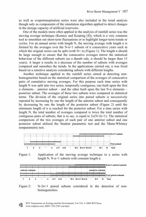
as well as evapotranspiration series were also included in the trend analysis though only as components of the simulation algorithm applied to detect changes in the storage capacity of artificial reservoirs. One of the models more often applied in the analysis of rainfall series was the moving average technique (Kenney and Keeping [4]), which is a very common tool to smoothen out short-term fluctuations or to highlight longer-term trends or cycles. For an annual series with length N, the moving average with length n is formed by the averages over the N-n+1 subsets of n consecutive years each in which the original series can be split (with N> n) (Figure 1). The length n should be large enough to ensure that the consecutive averages mirror the statistical behaviour of the different subsets (as a thumb rule, n should be larger than 15 years). A larger n results in a decrease of the number of subsets with averages compared and smoothes the trends. In the applications carried out, n was fixed based on a sensitive analysis considering subsets with different lengths. Another technique applied to the rainfall series aimed at detecting non-homogeneities based on the statistical comparison of the averages of consecutive pairs of cumulative moving averages. For this purpose each time series with length N was split into two series, temporally contiguous, one built upon the first n elements – anterior subset – and the other built upon the last N-n elements – posterior subset. The averages of these two subsets were compared in statistical terms. The division of the original series into paired subsets is successively repeated by increasing by one the length of the anterior subset and consequently by decreasing by one the length of the posterior subset (Figure 2) until the minimum length of n is reached for the posterior subset. For a time series with length N, the total number of averages compared is twice the total number of contiguous pairs of subsets, that is to say, is equal to 2x(N-2n+1). The statistical comparison of the two averages of each pair of one anterior subset and one posterior subset utilized the Student parametric test and the Mann-Whitney nonparametric test.

1 2 3 ... n n+1 n+2 ... N-n N-n+1 N-n+2 ... N-1 N Year

First subset

N-n+1 subset

Figure 1: Application of the moving average technique to a series with length N. N-n+1 subsets with constant length n.

anterior subsets posterior subsets

1 2 3 ... n n+1 n+2 ... N-n N-n+1 N-n+2 ... N-1 N Year

N-2n+1 paired subsets

First paired subsets

Figure 2: N-2n+1 paired subsets considered in the detection of non-homogeneities.




A non-homogeneity was considered to occur whenever at least one of the previous tests indicated that the two averages under comparison were statistically different. The analysis carried out showed two kinds of non-homogeneities: ones sporadic due to a period of time (a few years, seasons or months) with extremely high or extremely low rainfall and ones persisting and indicating successive posterior subsets with averages consistently different from the averages of the corresponding anterior subsets, thus, denoting a trend. In other words, a trend was considered to occur whenever persistent non-homogeneities were detected. The well known Mann-Kendall nonparametric test (Mann [5] and Kendall [3]), was also applied to detect trends in monthly and annual rainfall series. By applying the Sen slope estimator (Sen [12]), the trends thus detected were additionally characterized in terms of dimensionless magnitudes. In the three tests previously mentioned (Student, Mann-Whitney and Mann-Kendall tests) a significance level of α=5% was adopted (non-exceedance probability of 1-α/2=0.975 for bilateral or two-sided tests). The analysis of extreme rainfall events utilized annual maximum daily rainfall series – Pamd series – which were treated also by means of the moving average technique based on subsets with length n (Vaz [14]). The Pamd series are built upon one value per hydrologic year, the maximum rainfall amount in 24 h. The study also included the comparison of the N-n+1 probability distribution functions of the Gumbel law (Raynali and Salas [8]), obtained by considering separately each one of the N-n+1 consecutive subsets into which the Pamd series with length N was split. For each subset the probability distribution function was obtained by applying the method of moments based on the Weibull plotting position formula (Cunnane [1]). Along with the previous studies, the performance of artificial regulating reservoirs aiming at providing water for irrigation was also analyzed (Portela et al. [7] and Santos [10]). The models used for that purpose were more extensive and complex then the ones applied to rainfall data as they needed to account for the trends both in the inputs to the reservoirs (river flows) and in the outputs from the same (irrigation supplies). A monthly time step was adopted. As the stream flow series are generally not as long as the rainfall series, rainfall-runoff models were employed to extend the flow data, namely the soil sequential water budget and the Temez model (Temez [13]). To ascertain the trends in the crop water requirements long evapotranspiration series were established based on the Thornthwaite and on the Penman-Montheith models. Different supplies – in terms of volumes and guaranties/reliabilities – were considered. The analysis utilized computational simulation algorithms based on the mass equation.

3 Results

The moving average technique and the trend detection based on the identification of persistent non-homogeneities between consecutive pairs of anterior and posterior subsets were firstly applied to the rainfall series in the rain gages 1 to 11 schematically located in Figure 3 (Portela and Quintela [6]). For that purpose,




the year were analyzed. All the series were referred to the hydrologic or water year which, in Portugal, starts October 1st. The minimum length of each moving average was fixed at n=15 years which was also the minimum length of any anterior and posterior subset. The results achieved are exemplified in Figure 4, based on the 117-year rainfall series at Torre de Moncorvo gage (rain gage number 10).

Rain gage:1 - Góis2 - Penha Garcia3 - Pernes4 - Alter do Chão5 - Portalegre6 - Estremoz7 - Évora8 - Travancas9 - Cabeceiras de Basto10 - Torre de Moncorvo11 - Porto - Serra do Pilar12 - Vinhais13 - Serpa

SpainA

tla

nti

c O

cea

n

9

1

10

8

2

54

6

7

3

11

38º

42º

9º 7º 5º8º 6º

40º

12

13

Figure 3: Location of some of the rain gages considered in the trend analysis.

For a given period of time (year, season or month), the moving averages as well as the averages of the consecutive pairs of anterior and posterior subsets were made dimensionless by division by the average of the respective rainfall series in the total period of N=117 years. Each moving average was identified by the first year of the corresponding n=15-year period. The averages of each pair of anterior and posterior subsets were identified by the last year of the corresponding anterior subset. Figure 4 clearly shows that the rainfall series in March at Torre de Moncorvo exhibits a downwards trend which is also visible in the 2nd quarter of the hydrologic year, also as result from the decrease of the rainfall in March. For each one of the first 11 rain gages of Figure 3, Table 1 allows comparing the averages of the rainfall series in the recording periods and in the last 15 years analysed by Portela and Quintela [6]. It shows that all the rain gages exhibit notorious decreases in the rainfall in March. In annual terms, the last periods of 15 years were drier than the total recording periods. However, the decreases of the annual rainfall are within the natural variability of the phenomenon and, therefore, they do not represent non-homogeneities. To apply the Mann-Kendall test along with the Sen slope estimator 94 years of monthly and annual rainfall (from October 1910 to September 2004) in 144 Portuguese rain gages were selected (Santos and Portela [11]). Some of the series had sporadic gaps that were filled up based on linear regression analysis




(Yevjevich [15]). The Mann-Kendall test showed that most of the trends denoted by the 144 monthly and annual rainfall series were statistically meaningless, being explained by the natural temporal variability of the rainfall. Whenever the Mann-Kendall test pointed out a significant trend in a monthly or annual rainfall series the Sen estimator was applied to quantify the magnitude of such trend.

0.4

0.6

0.8

1.0

1.2

1.4

1878 1893 1908 1923 1938 1953 1968

First year of the 15-year moving averages

Moving average (-) b)

1892 1907 1922 1937 1952 1967Last year of the 15-year anterior subsets

Year

1st quarter

2nd quarter

March

a)

0.4

0.6

0.8

1.0

1.2


Year (October to September)

Average (-) c1)

0.4

0.6

0.8

1.0

1.2


1st quarter (October to December)

Average (-) c2)

0.4

0.6

0.8

1.0

1.2


2nd quarter (January to March)

Average (-) c3)

0.4

0.6

0.8

1.0

1.2


March

Average (-) c4)

Year 1st quarter 2nd quarter March

Anterior subset Posterior subset

Figure 4: Torre de Moncorvo rain gage. October 1878 to September 1995 (N=117 hydrologic years): a) dimensionless moving averages in 15-year periods; b) non-homogeneity occurrences; and c1) to c4) averages of the successive pairs of anterior and posterior subsets.

Table 1: First 11 rain gages of Figure 3. Average rainfalls in the recording periods and in the last 15-year periods.

Period PeriodYear 1st quarter 2nd quarter March Year 1st quarter 2nd quarter March(mm) (mm) (mm) (mm) (-) (-) (-) (-)

Góis 1917- 1999 1162 404 441 132 1985 - 1999 0.927 1.040 0.755 0.439Penha Garcia 1910 1999 803 306 289 89 1985 1999 0.976 1.123 0.800 0.368

Pernes 1915 1995 834 310 323 100 1981 1995 0.784 0.922 0.589 0.376Alter do Chão 1911 1999 625 224 236 72 1985 1999 1.028 1.212 0.820 0.436

Portalegre 1910 1997 854 312 325 101 1983 1997 0.975 1.105 0.762 0.436Estremoz 1911 1995 658 243 248 82 1981 1995 0.878 1.022 0.651 0.434

Évora 1900 1996 640 239 240 76 1982 1996 0.924 1.049 0.724 0.418Travancas 1913 1999 993 345 336 101 1985 1999 0.935 1.061 0.727 0.451

Cabeceiras Basto 1913 1999 1505 527 562 166 1985 1999 0.982 1.173 0.775 0.394Torre Moncorvo 1878 1995 563 204 173 54 1981 1995 0.882 1.012 0.614 0.442Porto-Serra Pilar 1900 1994 1187 440 415 127 1980 1994 0.985 1.075 0.796 0.651

Dimensionless average rainfallRain gageLast 15 years

(from October to September)

Recording periodAverage rainfall

(from October to September)




October November December January

April May

August September Year

March June

Atlantic Ocean

Atlantic Ocean

Atlantic Ocean

Atlantic Ocean

February

July

Figure 5: Trends in the monthly and annual rainfall series at 144 Portuguese rain gages. For each interval (month or hydrologic year) the scale represents the yearly variation (light grey for the increase and dark grey for the decrease) of the rainfall, expressed in percentage of the mean annual rainfall in that time interval. The dots represent the 144 rain gages utilized in the study.

By means of a GIS, maps with the spatial distribution (based on the krigging interpolation method) of the Sen estimator were produced, as shown in Figure 5 in which the dots represent the 144 rain gages considered in the study. Any value from one of the maps in Figure 5 represents a change (increase or decrease) in the annual amount of rainfall expressed in percentage of the mean annual rainfall in the period to which the map under consideration refers. The figure clearly shows that most of the rainfall changes are spatially quite circumscript and almost neglectable. Only the rainfall in March exhibits a very pronounced and widespread downwards trend. However, it should be said that except for a small region in the North of Portugal, the rainfall in March is always smaller than




150 mm which means that a maximum annual decrease according to the Sen estimator of about 1.3% will, in fact, represent a decrease of the annual amount of rainfall in March of only 2 mm. To analyze the effect of considering different periods in the estimates of the annual maximum daily rainfall given by the Gumbel law, the Pamd series at 24 rain gages were analyzed (Vaz [14]). The results achieved for the recording period of 70 years (from October 1931 to September 2001) in three of those rain gages are exemplified in Figure 6 (rain gages numbers 3, 12 and 13 in Figure 3). In each rain gage the Gumbel cumulative distribution was computed based on each one of the successive subsets of 25 consecutive years each (total number of subsets of 70-25+1=46). For each of the three rain gages, Figure 6 contains the representation of the Gumbel cumulative distribution based on the first five and on the last five subsets of 25-year each. The vertical axes were made dimensionless by dividing the estimates of the maximum annual daily rainfall by the average of the Pamd sample in the 70-year period and the horizontal axes represent non-exceedance probability, F. The estimates of Pamd for the non-exceedance probability of 0.99 (100-year return period) are highlighted.

0

1

2

3

-3 -2 -1 0 1 2 3

Pamd/(Pamd)average

Pernes

a)

b)

0.01 0.2 0.5 0.8 0.95 0.99 F

0

1

2

3

-3 -2 -1 0 1 2 3

Serpa

Pamd/(Pamd)average

0.01 0.2 0.5 0.8 0.95 0.99 F

a)

b)

0

1

2

3Vinhais

Pamd/(Pamd)average

0.01 0.2 0.5 0.8 0.95 0.99 F

a)

b)

Series order: a) Dark blue to light blue: first five 25-year series ( 1 2 3 4 5 )

b) Yellow to brown: last five 25-year series ( 42 43 44 45 46 )

Figure 6: Application of the Gumbel law based on different recording periods.

Figure 6 shows that for Vinhais gage the estimates based on the latest records are not as high as those supported by the oldest records. The opposite situation occurs in Serpa gage while in Pernes both estimates are very close. One of the conclusions that can be drawn out based on the results exemplified in Figure 6 is that different periods need to be analyzed in order to ensure safe/conservative design criteria. Another conclusion is that the behaviour of the extreme rainfall time series may refuse (like in Vinhais or even in Pernes) or confirm (like in Serpa) the upwards trend that is generally pointed out as denoting the climate change effect. Due to the temporal irregularity that characterizes the Portuguese hydrologic regime, most of the water supplies are ensured by artificial reservoirs created by dams, a significant part of these infrastructures having been built in the 1950 and 1960 decades. So, a question arises: if the climate is changing are those old reservoirs still able to ensure the amount of water adopted as design criterion




with the guaranty/reliability required by each type of water use? This question is especially pertinent when considering reservoirs for irrigation purposes as both the crop demand and the water availability may be influenced by the trends exhibited by the hydrologic variables. To answer the previous question, the performance of 10 hypothetical irrigation reservoirs was analyzed, by means of computational simulation techniques based on 94 years of monthly inflows and of crop requirements (from October 1910 until September 2004) (Portela et al. [7] and Santos [10]). Some of the trends thus detected are depicted in the Figure 7. The dark grey arrows denote worse constraints – decrease (-) of the inflows to the reservoir or greater (+) storage capacities to ensure the same water supply with the same guaranty – and the light grey arrows better constraints – increase (+) of the inflows to the reservoir or smaller (-) storage capacities to ensure a given water supply with a given guaranty. The water supplies were expressed in percentage of the mean annual inflows and guaranties of 80 and 90% were considered. On a monthly basis, the guaranty can be understood as the percentage of months with total fulfilment of the water requirements. The guaranty applied to the irrigation supply is generally 80%.

30 50 70 30 50 70

Vinhais-Qta da Ranca + - - - + - -Castro Daire - + + + + + +Cabriz - - - - + - -Vale Giestoso + - - - - - -Cunhas - + + + + + +

Centre Portugal Couto de Andreiros - + + + + + +Torrão do Alentejo - + + + + + +Albernoa + + + + + + +Monte da Ponte + + + + + + +Vascão + - - + - - +

Trend in the storage capacity as a function of the water demand and of the guaranty of the water supply

Water demand (% of mean annual inflow)

Guaranty of water supply80% 90%

Case studyTrend in the mean annuall

inflow

North Portugal

South Portugal

Figure 7: Irrigation reservoirs. Trend detection and guaranty of the water supplies.

Figure 7 shows that most of the case studies – with special emphasis on those located in the centre and in the southern regions of Portugal – denote loss of reliability as more storage capacity would presently be required to ensure the same water demand with a given guaranty. In some of the case studies this even happens when increases of the water inflows occurred. However, it should be pointed out that all the increases/decreases under consideration were very small and often almost negligible.

4 Final remarks: planning under uncertainty

In general terms the studies developed until now showed that some of the hydrologic series are much more resilient than the human perception and that it




is difficult, for the time being, to clearly identify signs of the climate changes in such series. This also suggests that further studies and scientific judgments are required as, somehow, there is a gap between what is already considered as resulting from the climate change and the effective behaviour denoted by some of the hydrologic time series. But does this mean that the stationarity assumption of most of the hydrologic models is no longer valid? Will the future be statistically different from the past and if so how can we introduce this dissimilarity in the hydrologic models and in the design criteria? Though for the time being this is still an unsolved question it undoubtedly points towards the need to account for hydrologic uncertainty, for instance, by means of risk analysis tools based on scenarios.

References

[1] Cunnane, C., 1978, ‘Unbiased plotting positions - a review’, Journal of Hydrology (37), 205-222.

[2] IPCC, 2007, Fourth Assessment Report: Climate Change 2007, http://www.ipcc.ch/ipccreports/assessments-reports.htm

[3] Kendall, M. G., 1975, Rank Correlation Methods, 4th ed., Charles Griffin: London.

[4] Kenney, J. F.; Keeping, E. S., 1962, "Moving Averages." §14.2 in Mathematics of Statistics, Pt. 1, 3rd ed. Princeton, NJ: Van Nostrand, pp. 221-223.

[5] Mann, H. B., 1945, “Non-parametric test against trend”, Econometrica, 13, 245-259.

[6] Portela, M. M; Quintela, A. C., 2001, “A diminuição da precipitação em épocas do ano como indício de mudança climática. Casos estudados em Portugal Continental”. Ingeniéria del Agua, Vol. 8(1), pp. 79-92, ISSN 1134-2196, Spain (in Portuguese).

[7] Portela, M. M.; Santos, J.; Coelho, M. F., 2006, “Alterações em séries de variáveis hidrológicas: seus efeitos nos volumes de água a fornecer para rega e na fiabilidade do fornecimento desses volumes a partir de albufeiras”. 8º Congresso da Água, 19 p., Associação Portuguesa dos Recursos Hídricos (APRH), Figueira da Foz, Portugal (in Portuguese).

[8] Raynali, J. A.; Salas, J. D., 1986, “Estimation procedures for the type-1 extreme value distribution”, Journal of Hydrology (87), 315-336.

[9] Santos, F. D; Miranda, P. M. (eds.), 2008 Alterações climáticas em Portugal. Cenários, impactos e medidas de adaptação. Projecto SIAM, Gradiva, Lisboa (in Portuguese).

[10] Santos, J. F., 2008, Alterações em séries de variáveis hidro-climatológicas: seus efeitos nos volumes de água a fornecer para rega e na fiabilidade do fornecimento desses volumes a partir de albufeiras, MSc Thesis. IST, Lisbon, Portugal (in Portuguese).

[11] Santos, J. F.; Portela, M. M., 2008, “Quantificação de tendências em séries de precipitação mensal e anual em Portugal Continental”, VIII Seminário




Ibero-Americano sobre Sistemas de Abastecimento Urbano, SEREA 2008, IST, Lisbon, Portugal (in Portuguese).

[12] Sen, P. K., 1968, “Estimates of the regression coefficient based on Kendall's Tau”, J. Am. Stat. Assoc., 63, 1379-1389.

[13] Temez, J.R., 1977, Modelo matemático de transformación precipitación- -aportación. ASINEL

[14] Vaz, C. M., 2008, Análise de tendências em séries de precipitação diária máxima anual. MSc Thesis, IST, Lisbon, Portugal (in Portuguese).

[15] Yevjevich, V., 1972, Probability and statistics in Hydrology, Water Resources Publications, Fort Collins, Colorado, USA.




Trends in hydrologic time series - WIT Press

Documents

Transcript of Trends in hydrologic time series - WIT Press