Treasury Yield Implied Volatility and Real Activity

Martijn Cremers1 Matthias Fleckenstein2 Priyank Gandhi1

1University of Notre Dame

2University of Delaware

AEA Annual MeetingsJanuary, 2018

1 / 24

Introduction

Research question:

What information from financial markets predicts level and volatility of realactivity?

Intuition: Financial markets are forward-looking – potentially capture futureeconomic expectation

Important for policymakers: Incorporate financial market variables in earlywarning systems

Important for investors: Could inform asset prices

2 / 24

Introduction

Not the first to ask this question:

Many papers examining link between stock / bond markets and future realactivity

Comprehensive literature review: Stock and Watson (2003):More than 100 papers

Over past 15 years

More than 43 financial variables

Many samples – 17 different countries

3 / 24

Introduction

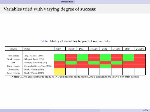
Variables tried with varying degree of success:

Table: Ability of variables to predict real activity

Variable Paper GDP σ(GDP) IND σ(IND) CON σ(CON) EMP σ(EMP)

Term spread Ang/Piazzesi (2003)

Stock returns Schwert; Fama (1990)

VIX Bekaert/Hoerova (2014)

Bond returns Connolly/Stivers/Sun (2006)

Commodity Stock/Watson (2013)

Forex returns Stock/Watson (2013)

Notes: GDP is gross domestic product; IND is industrial production; CON is consumption; EMP is non-farm payroll

4 / 24

Introduction

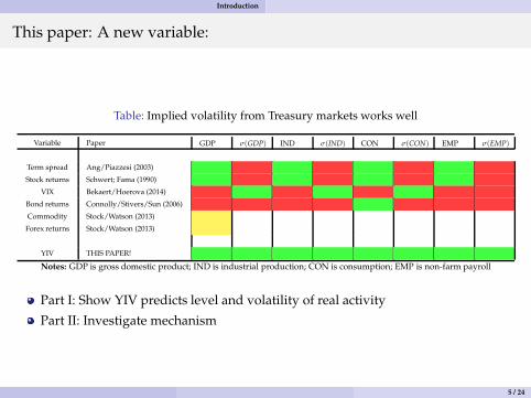
This paper: A new variable:

Table: Implied volatility from Treasury markets works well

Variable Paper GDP σ(GDP) IND σ(IND) CON σ(CON) EMP σ(EMP)

Term spread Ang/Piazzesi (2003)

Stock returns Schwert; Fama (1990)

VIX Bekaert/Hoerova (2014)

Bond returns Connolly/Stivers/Sun (2006)

Commodity Stock/Watson (2013)

Forex returns Stock/Watson (2013)

YIV THIS PAPER!

Notes: GDP is gross domestic product; IND is industrial production; CON is consumption; EMP is non-farm payroll

Part I: Show YIV predicts level and volatility of real activity

Part II: Investigate mechanism

5 / 24

Introduction

YIV is a good candidate variable:

Intuitive reason: Market for Treasury bonds and notes and related options andfutures is largest / most liquid

Theoretical reason: Models (Bansal / Zhou (2005); Ang / Bekaert (2002); Dai /Singleton (2002); Dai / Singleton / Yang (2007) etc.) suggest interest rate volatilityvaries over the business cycles

Surprisingly limited research that uses interest rate uncertainty!

6 / 24

Data

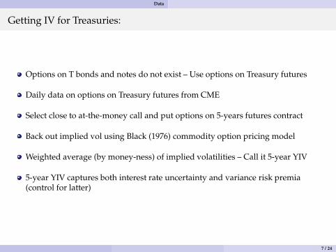
Getting IV for Treasuries:

Options on T bonds and notes do not exist – Use options on Treasury futures

Daily data on options on Treasury futures from CME

Select close to at-the-money call and put options on 5-years futures contract

Back out implied vol using Black (1976) commodity option pricing model

Weighted average (by money-ness) of implied volatilities – Call it 5-year YIV

5-year YIV captures both interest rate uncertainty and variance risk premia(control for latter)

7 / 24

Data

Summary statistics and correlations:

Table: 1, 2: Summary statistics and correlations.

Mean σ Min 25th Median 75th Max ρ

5-year YIV 3.38 1.17 1.37 2.71 3.12 3.67 9.21 0.71

GDP IND CON EMP TRM ∆SY ITB VIX UNC

5-year YIV -0.54∗∗∗ -0.45∗∗∗ -0.41∗∗∗ -0.57∗∗∗ 0.18∗∗∗ -0.12∗∗ 0.04 0.49∗∗∗ 0.12∗∗

Notes: Summary statistics for the YIV; GDP is gross domestic product; IND is industrial production; CON is consumption; EMPis non-farm payroll; TRM is term spread; ∆SY is short-rate; ITB is Treasury bond returns; VWR is value-weighted stock returns;VIX is the CBOE Volatility Index; UNC Bloom/Baker/Davis (2015) uncertainty index; Monthly data except for GDP (quarterly);

Monthly data, 1990 - 2015.

8 / 24

Results I: Predicting macroeconomic activity levels and volatility

Empirical framework: Predictive regressions:

j=H

∑j=1

log(1 + MACROi,t+j)/H = αH + βHYIV + Controls + ǫt+H

Horizons of 1 - 36 months

Newey-West / Hansen-Hodrick standard errors (1 - 36) lags

Control for lags as well as standard predictor variables (term-spread, short rate,VIX, bond returns, stock returns, etc.)

9 / 24

Results I: Predicting macroeconomic activity levels and volatility

YIV predicts real activity:

Table: 4, A3, A4, A5, A6: Predicting real activity: Coefficient on YIV

H = 12 18 24 30 36

GDP -0.08∗∗∗ -0.07∗∗∗ -0.05∗∗∗ -0.05∗∗∗ -0.04∗∗∗

(-3.61) (-3.46) (-3.83) (-3.99) (-3.72)

R2 34.42 26.80 20.72 17.12 14.72

IND -0.17∗∗∗ -0.12∗∗∗ -0.09∗∗∗ -0.06∗∗∗ -0.05∗∗

(-2.90) (-2.61) (-2.66) (-2.48) (-2.00)

R2 32.13 20.47 11.75 7.20 4.87

CON -0.09∗∗∗ -0.07∗∗∗ -0.06∗∗∗ -0.05∗∗∗ -0.05∗∗∗

(-3.31) (-3.19) (-3.36) (-3.52) (-3.76)

R2 34.48 27.76 21.63 17.58 16.11

EMP -0.09∗∗∗ -0.08∗∗∗ -0.07∗∗∗ -0.05∗∗∗ -0.04∗∗∗

(-6.25) (-5.36) (-4.97) (-4.71) (-4.06)

R2 44.77 38.55 29.40 21.78 15.52

Notes: Dependent is year-on-year growth rate in the GDP, IND, CON, EMP; Controls include the term spread; changes inshort-rate; Treasury bond returns; Corporate bonds returns; Stock index returns; CBOE Volatility Index; Economic uncertainty

from Baker/Bloom/Davis (2015); Quarterly or monthly data, 1990 - 2016.

10 / 24

Results I: Predicting macroeconomic activity levels and volatility

YIV predicts volatility of real activity:

Table: 5, A7, A8, A9, A10: Predicting GDP, IP, CON, EMP volatility: Coefficient on YIV

H = 12 18 24 30 36

GDP 0.25∗∗∗ 0.30∗∗∗ 0.30∗∗ 0.26∗∗ 0.20∗∗

(2.95) (2.71) (2.30) (2.12) (2.03)

R2 25.35 26.99 27.45 29.19 30.60

IND 0.82∗∗∗ 1.06∗∗∗ 1.14∗∗∗ 1.02∗∗∗ 0.82∗∗∗

(3.60) (3.31) (3.04) (2.84) (2.49)

R2 36.33 34.29 31.41 23.86 16.21

CON 0.28∗∗∗ 0.33∗∗∗ 0.33∗∗∗ 0.30∗∗∗ 0.26∗∗∗

(4.06) (3.37) (3.08) (2.90) (2.53)

R2 30.69 25.53 20.34 16.58 13.10

EMP 0.22∗∗∗ 0.26∗∗∗ 0.29∗∗∗ 0.29∗∗∗ 0.27∗∗∗

(5.04) (4.19) (3.74) (3.52) (3.13)

R2 35.48 29.74 24.36 20.34 16.47

Notes: Dependent is year-on-year volatility of IP, CON, EMP; Quarterly or monthly data, 1990 - 2016.

11 / 24

Results I: Predicting macroeconomic activity levels and volatility

Results robust to a battery of tests:

Predict over short- and long-term

Not driven by variance risk premia

Using non-overlapping data

Excluding financial crisis

Out of sample forecasts

Obvious question: Why does this work so well?

12 / 24

Results II: YIV captures interest rate uncertainty

YIV captures interest rate volatility (uncertainty) I:

Table: 3: Predicts interest rate volatility

H = 12 18 24 30 36

2-year rates 1.45∗∗ 1.06∗ 0.63 0.27 -0.26

(1.98) (1.75) (0.84) (0.29) (-0.23)

R2− ord 6.02 2.33 0.61 0.09 0.07

5-year rates 1.22∗∗∗ 1.11∗∗ 1.02∗∗ 1.34∗∗∗ 1.66∗∗∗

(2.33) (2.24) (2.06) (2.43) (2.49)

R2− ord 8.01 6.01 4.71 7.43 10.08

10-year rates 0.63 0.66 0.72 1.17∗∗ 1.73∗∗∗

(1.57) (1.38) (1.48) (2.23) (3.20)

R2− ord 4.28 3.75 3.91 9.12 17.91

Notes: Dependent is realized future volatility of 2-, 5-, 10-year rates.

13 / 24

Results II: YIV captures interest rate uncertainty

YIV captures interest rate volatility (uncertainty) II:

Figure: 2: Response of YIV to monetary policy surprises

-2 -1 0 1 20.7590

0.8797

1.0003

1.1209

1.2416

1.3622Positive Surprises

-2 -1 0 1 20.7590

0.8797

1.0003

1.1209

1.2416

1.3622Negative Surprises

-2 -1 0 1 20.7590

0.8797

1.0003

1.1209

1.2416

1.3622No Surprises

YIV Short-rate VIX

Notes: YIV, the short rate, and the term spread over a 5-day window around Fed’s announcements regarding changes in the Federal Funds rate; Daily data,1990 - 2016.

YIV increases on both unexpected rate cuts and increases

14 / 24

Results III: Mechanism

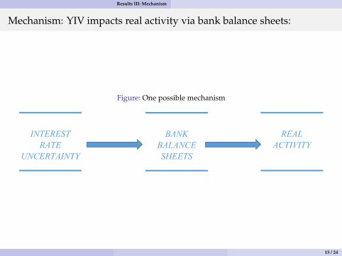
Mechanism: YIV impacts real activity via bank balance sheets:

Figure: One possible mechanism

INTEREST

RATE

UNCERTAINTY

BANK

BALANCE

SHEETS

REAL

ACTIVITY

15 / 24

Results III: Mechanism

Bank centric view of interest rate risk:

Banks’ core activities deposits-taking and loans exposes their balance sheets tointerest rate risk

Banks cannot completely immunize themselves from interest rate uncertainty /risk

Interest rate uncertainty impacts bank liabilities → assets → net worth → realactivity

Drechsler/Savov/Schnabl (2017): Monetary policy affects real activity via bankdeposits

Haddad/Sraer (2017): Bank interest rate exposure forecasts bond returns

16 / 24

Results III: Mechanism

Support for our mechanism:

Evidence 1: YIV forecasts lower (higher) demand (volatility) for deposits frombanks

Evidence 2: YIV forecasts cost of capital of banks

Evidence 3: YIV forecasts level and volatility of bank credit

Evidence 4: Stronger forecasts for banks more exposed to IR risk

Evidence 5: YIV forecasts investment for bank dependent firms

17 / 24

Results III: Mechanism

Evidence 1: YIV and bank deposits:

Table: 6: Predicting bank deposits

H = 12 18 24 30 36

Bank deposit -0.25∗∗∗ -0.27∗∗∗ -0.28∗∗∗ -0.28∗∗∗ -0.29∗∗∗

(-3.31) (-4.19) (-4.70) (-4.66) (-4.36)

Bank deposit volatility 0.62∗∗∗ 0.45∗∗∗ 0.25∗ 0.18 0.12

(2.64) (2.68) (1.64) (0.98) (0.62)

Notes: Dependent is bank deposit growth and bank deposit volatility; Monthly data, 1990 - 2016.

18 / 24

Results III: Mechanism

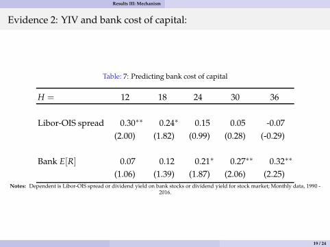
Evidence 2: YIV and bank cost of capital:

Table: 7: Predicting bank cost of capital

H = 12 18 24 30 36

Libor-OIS spread 0.30∗∗ 0.24∗ 0.15 0.05 -0.07

(2.00) (1.82) (0.99) (0.28) (-0.29)

Bank E[R] 0.07 0.12 0.21∗ 0.27∗∗ 0.32∗∗

(1.06) (1.39) (1.87) (2.06) (2.25)Notes: Dependent is Libor-OIS spread or dividend yield on bank stocks or dividend yield for stock market; Monthly data, 1990 -

2016.

19 / 24

Results III: Mechanism

Evidence 3: YIV and bank credit:

Table: 8: Predicting bank credit

H = 12 18 24 30 36

Bank credit -0.13∗∗∗ -0.14∗∗∗ -0.14∗∗∗ -0.14∗∗∗ -0.14∗∗∗

(-3.07) (-4.30) (-4.42) (-4.51) (-5.06)

Bank credit volatility 0.61∗∗∗ 0.73∗∗∗ 0.60∗∗∗ 0.46∗∗∗ 0.33∗∗∗

(7.02) (5.47) (4.75) (4.51) (3.52)

Notes: Dependent is bank credit growth and bank credit volatility; Monthly data, 1990 - 2016.

20 / 24

Results III: Mechanism

Evidence 4: YIV and bank credit by exposure to IR risk:

Table: 9: Predicting bank credit by exposure to interest rate risk

H = 12 18 24 30 36

Small banks, Low Exp. -0.26∗∗∗ -0.28∗∗∗ -0.28∗∗∗ -0.28∗∗∗ -0.25∗∗∗

(-2.79) (-3.90) (-4.40) (-4.90) (-4.16)

Small banks, High Exp. -1.66∗∗ -1.99∗∗ -2.16∗∗ -2.36∗∗ -2.56∗∗

(-2.01) (-1.99) (-2.08) (-2.20) (-2.35)

Large banks, Low Exp. -0.18 -0.07 -0.01 -0.02 0.01

(-0.59) (-0.28) (-0.01) (-0.09) (0.03)

Large banks, High Exp. -0.31∗∗∗ -0.37∗∗∗ -0.39∗∗∗ -0.38∗∗∗ -0.35∗∗

(-2.59) (-2.76) (-2.60) (-2.46) (-2.16)

Notes: IR derivatives held for trading used to compute IR exposure (Purnanandam(2007)); Dependent is bank credit growth;Quarterly data, 1990 - 2016.

21 / 24

Results III: Mechanism

Evidence 5: YIV and investment growth:

Table: 10: Predicting firm investment by bank dependence

H = 12 18 24 30 36

Bank dependent firms -0.28∗ -0.22 -0.22 -0.34∗ -0.31∗

(-1.80) (-1.44) (-1.48) (-1.72) (-1.47)

Non-bank dependent firms 0.00 0.00 -0.01 -0.03 -0.05

(0.00) (0.01) (-0.14) (-0.37) (-0.48)

Notes: Dependent is capex growth; Quarterly data, 1990 - 2016.

Interest rate uncertainty predicts aggregate capex (Mueller / Vedolin (2017)

22 / 24

Conclusion

Key results:

I: A simple measure of uncertainty from Treasury derivatives markets predictslevel and volatility of macroeconomic activity

II: Over horizons of 1 - 36 months

III: Robust to a variety of specifications

23 / 24

Conclusion

Contribution:

Variable captures interest rate uncertainty

Directly impacts balance sheet of banks

Establish a link between time-varying uncertainty in US Treasury markets andbalance sheet of banks that impacts real activity

24 / 24