Trapping and cooling of ions - Accueil - CEL

HAL Id: cel-00334152https://cel.archives-ouvertes.fr/cel-00334152

Submitted on 24 Oct 2008

HAL is a multi-disciplinary open accessarchive for the deposit and dissemination of sci-entific research documents, whether they are pub-lished or not. The documents may come fromteaching and research institutions in France orabroad, or from public or private research centers.

L’archive ouverte pluridisciplinaire HAL, estdestinée au dépôt et à la diffusion de documentsscientifiques de niveau recherche, publiés ou non,émanant des établissements d’enseignement et derecherche français ou étrangers, des laboratoirespublics ou privés.

Trapping and cooling of ionsCaroline Champenois

To cite this version:Caroline Champenois. Trapping and cooling of ions. DEA. du 6 au 10 octobre a l’ecole de Physiquedes Houches,ecole predocotorale sur les atomes froids et la condensation de Bose-Einstein, 2008, pp.28.cel-00334152

https://cel.archives-ouvertes.fr/cel-00334152

https://hal.archives-ouvertes.fr

C. Champenois, trapping and cooling of ions, 2008 Les Houches predoc-school 1

These notes are part of the five lessons given in Les Houches on october 2008 for the

cold atom and BEC predoc school. Why a lesson about trapped ions in such a school?

There is no BEC, no degenerate gas, no Mott transition with trapped ions...but there

are optical clocks among the most accurate in the world, there is phase transition from

liquide to crystal, there are cold molecules to study cold reactions and most famous of all,

there is the realisation of quantum gates, the bricks of quantum computer. Furthermore,

experiments done with trapped ions have inspired and initiated several breakthroughs

with neutral atoms because with such a system, “your hands are free”, the trap keeps the

ion(s) for you and you can try many different laser interaction protocoles. Here are the

basics that, I hope, will help you understand why experiments with trapped ions can be

so interested.

1 Confining charged particules with oscillating elec-

tric fields

1.1 The adiabatic approximation

Because of the Laplace law ruling a space free of charge (∆V = 0), it is not possible to

trap a charged particule only by static electric field. For example, if by a set of electrodes

a confining harmonic potential is created in the (x, y) plane, it has to be non-confining in

the z direction:

Φ(x, y, z) = A(x2 + y2 − 2z2) (1)

The idea of W. Paul was to use an oscillating potential

Φrf (x, y, z, t) = A(x2 + y2 − 2z2) cos(Ωt) (2)

more generally, the potential is the sum of a radiofrequency and a static contribution:

Φ(r, t) = Φrf (r, t) + Φs(r, t) (3)

The first radiofrequency ion trap worked in 1954 and the first paper where its principle

was described was written by W. Paul in 1956 and mentionned an “ionenkafig”. Wolfgang

Paul and Hans Dehmelt won the Nobel prize in physics in 1989 “For the development of

the ion trap technique”.

To understand the motion of an ion inside such a potential, let’s first assume there is

no static voltage (Φs(r) = 0). If the time oscillating electric field E0(r) cos(Ωt) is uniform

(E0(r) = E0), then the motion is simply a rf driven motion at frequency Ω:

r(t) = − qE0

mΩ2cos(Ωt) = −a cos(Ωt) (4)

But if E0(r) is non uniform, the motion can be interpreted as the sum of a slow motion

induced by the enveloppe of the rf field and the rf driven motion which has an amplitude


depending on the local rf field.

r(t) = R0(t)︸︷︷︸

slow

+ R1(t)︸︷︷︸

−a(t) cos(Ωt)

(5)

the local electric field ruling the equations of motion can be written like:

E0(r(t)) = E0(R0) − (a.∇)E0(R0) cos(Ωt) + · · · (6)

A simple resolution can be reached by two approximations:

• a first order development of E0 around R0.

• the adiabatic approximation assuming that : the typical evolution time scale of

a and R0 is far longer than the rf period.

with a(t) = a(R0(t)) put into the equation, one can easily show that

mR0 = − Q2

4mΩ2grad(E2

0). (7)

It says that as far as R0(t) is concerned, it is like the particle is trapped in a static

potential well called the pseudopotential:

V ∗(r) =Q2E2

0(r)

4mΩ2. (8)

If the static electric field is switched on again, the superposition principle leads to the

effective potential

V ∗eff (r) =

Q2E20(r)

4mΩ2+ qΦs(r) (9)

and the motion in this potential gives R0(t). The rf-driven motion (µmotion) is deduced

by

R1(t) = −QE0(R0)

mΩ2cos(Ωt) (10)

The potential V ∗(r) effectively traps if E20(r) increases with r (this condition is not suffi-

cient, see further). So the further is the ion from the center of the trap, the larger is the

µmotion. The µmotion being a driven motion proportionnal to the local field, it can not

be cooled.

1.2 Choosing a geometry, the quadrupole as a generator of har-

monic potential

Let’s go back to our first goal: create a harmonic trapping potential in 3D for a charged

particle. Now, we know we have to make a detour to rf field and make sure that E20(r)

and Φs(r) behave like (x2, y2, z2). This is reached if

Φrf (r, t) = −(αx2 + βy2 + γz2) cos(Ωt). (11)


Figure 1: On the left, equipotential in the x − y plane of a indeal 3D Paul trap (axis of

symmetry: Oz). in the center, equipotential in the x− z plane for the same trap, on the

right, equipotential in the x− y plane of an ideal linear rf-trap.

with α + β + γ = 0. Two geometries with two different symmetries are used; the 3D

cylindrical trap where α = β = −γ/2 and the 2D translational symmetry where α =

−β, γ = 0 and where a static voltage is required to trap along the Oz axis (see figure 1 for

equipotential lines in both geometries). Let’s first deal with the 3D geometry, many points

can be extrapolated to the 2D linear geometry. In 3D, the ideal geometry is a ring plus

two endcaps. If a static voltage is added to the rf voltage and both are applied between

the ring and the two endcaps, the potential voltage created between the electrodes can

be described by

Φ(r, t) = (V0 cos(Ωt) + Vs)x2 + y2 − 2z2

2r20

. (12)

where r0 is the radius of the trap (see figure 2). Such a voltage repartition can be

produced if the surfaces of the electrodes exactly match an equipotential surface which is

an hyperboloid of revolution (x2 − 2z2 =constante)(see fig 2).

But even if the trap is perfectly machined, it is never like in the equations, simply

because the trap has a finite size. Today, several experiments even use miniature (see fig

2, right) and micro traps which do not obey the perfect geometry required by equations.

Nevertheless, as long as some symmetry principles are obeyed, in the center of the trap,

the potential created by the electrodes can be approximated by equation (12). Getting

further from the trap center, higher order contributions become non negligeable. This is

of importance for experiments with a large set of ions, where areas far from the center

are visited by the ions.

In the following, we assume Eq (12) is a good representation of the voltage. In the

adiabatic approximation, the effective potential is then

V ∗eff (r) =

Q2V 20

4mΩ2r40

(x2 + y2 + 4z2) +QVs2r2

0

(x2 + y2 − 2z2) (13)

(here we use the convention where V0 and Vs are potential differences between the ring

and the end-caps forming the trap). Inside this harmonic potential, the motion can be


Figure 2: On the left, a Paul trap like shown by Paul in his Nobel lecture, 2r0 is the

smallest inner diameter of the ring. For an ideal geometry, the height 2z0 between the

two endcaps should be equal to 2√

2r0. On the right, an example of a miniature trap, the

ring inner diameter is 1.4 mm.

described by two frequencies of motion (one for x, y and one for z). Some parameters are

very useful to define these frequencies and other things:

qx = − 2QV0

mΩ2r20

; qz =4QVsmΩ2r2

0

(14)

ax =4QVsmΩ2r2

0

; az = − 8QVsmΩ2r2

0

(15)

From these parameters, the frequencies of motion can be expressed like:

ωx =Ω

2

√

ax + q2x/2 ; ωz =

Ω

2

√

az + q2z/2 (16)

Following our construction of macro and micromotion, the equation of motion of a single

ion in such a trap is then

x(t) = X cos(ωxt)(

1 +qx2

cos(Ωt))

(17)

1.3 Beyond the adiabatic approximation

In the particular case of a quadrupolar geometry (where the pseudopotential is harmonic),

the complete equations of motion for a single ion can be solved analytically, without

any approximation. In a potential described by Eq 12, the equations of motion are linear

and uncoupled in the spatial coordinates (it is not true for higher order geometries). So

each coordinates can be studied independantly:

x = − Qx

mr20

(V0 cos Ωt+ Vs) (18)


Figure 3: Stability region of the Mathieu equation where rf traps are operated, left: 3D

Paul trap, right: linear trap.

the introduction of the reduced time scale ξ = Ωt/2 leads to the well-known Mathieu

equationd2x

dξ2+ (ax − 2qx cos(Ωt))x(ξ) = 0 (19)

which belongs to the family of differential equations with periodic coefficients. Solutions of

this equation can be found in many math textbooks. The important points to remember

are

• the solutions have the form

x(t) = Aeiωxt∑

n

C2neinΩt +Be−iωxt

∑

n

C2ne−inΩt (20)

with ωx = βxΩ/2, βx depending only on ax and qx.

• these solutions are stable if the 0 ≤ βi ≤ 1. This condition defines areas in the plane

defined by (ax,qx) or (az,qz): the stability regions. In practise, rf traps are operated

in the lowest stability region (the one including (0,0), see figure 3).

The solutions of the Mathieu equation can be expanded in the lowest order approx-

imation which requires (|ax|, q2x) ≪ 1 and then βx ≪ 1. In this limit

βx =

√

ax +q2x

2(21)

and

x(t) = X cos(ωxt)(

1 +qx2

cos Ωt)

(22)


Figure 4: Left: plot of equation X cos(ωxt)(

1 + qx2

cos Ωt)

for qx = 0.2 and 0.4. Right:

plot of the same equation with X cosωxt → X(ǫx + cosωxt) which includes an excess

micromotion characterized by ǫx = 0.25.

this is exactly the equation obtained in the adiabatic approximation. To have a look at

examples of trajectories, go to figure 4. For an ideal 3D Paul trap, az = −2ax,y and

qz = −2qx,y. This implies, for example, that if Vs = 0, ωz = 2ωx.

As soon as there is more than one ion in the trap, the Mathieu equation does

not describe exactly the motion of the ions because it does not include the Coulomb

repulsion. This repulsion becomes important when ions are cooled and when the ion-

ion distance is reduced. Then, the equations of motion become nonlinear. The non-

linearities can manifest themselves by nonlinear resonance coupling the motion along x,y

and z or coupling these motions to the radiofrequency. For some working parameters,

the trajectories are then unstable, even inside the stability diagram. Imperfections in the

shape of the electrodes can have the same effects.

1.4 Another tool to trap charged particles: the Penning trap

This device, invented by Penning already in 1936 makes use of a large magnetic field

superposed to a static voltage applied on electrodes. The geometry can be a cylinder

with two endcaps but many experiments now use the hyperboloid of revolution already

defined for the Paul trap. The motion is characterized by three frequencies of motion.

The oscillation in the static confining potential along Oz and two frequencies of motion

for the plane x− y, related to the cyclotron and magnetron motion.

This device is very famous for the high precision measurement of g−2 for the electron

(the first ones from 1969 to 1977 by Graff and Dehmelt and the last one in 2006 by the

group of Gabrielse (Harvard)). The other application of Penning trap is high precision

mass measurement where the precision is such that the mass difference between isobare

can now be exploited.

Because of the required high magnetic field, Penning traps are not very appropriate

for most high precision spectroscopic measurements as a small relative fluctuation of the


magnetic field induces too high frequency fluctuations in the transition). To know more

about them, refer to the books speaking about charged particle traps.

2 Interaction of light with ions trapped in a rf quadupole

trap

When a high number of ions is trapped and the motion can no more be described by

a harmonic oscillator+µmotion, the ion-light interaction is very similar to the ones of

unbound atoms and concepts and processes known for neutral atom work roughly in the

same way (Doppler cooling...). The situation becomes peculiar for single ion or single

ions (a chain in a linear trap) which are trapped at the node of the rf field. Furthermore,

if traps are operated with ax and q2x ≪ 1 the motion can be very well described by

a harmonic oscillator. Then, it becomes possible to coherently couple the internal and

external degrees of freedom. Indeed, the Hamiltonian of the system can, in this limit,

be equivalent to the Jaynes-Cummings Hamiltonian describing photons in QED cavity

and several experiments with trapped ions have been inspired by this analogy (creation

of non-classical states of vibration, coherent states...). In this section, we consider single

ion(s) in quadrupole traps where the oscillation is characterized by ωx, ωy, ωz and most of

the time, we treat the atom as a two level system.

2.1 Classical treatment of the motion

The atom is considered as a two level system |g〉, |e〉 with internal energy Ee−Eg = hω0.

The Hamiltonian of the non-interacting atom is

H0 =hω0

2(|e〉〈e| − |g〉〈g|) +

p2

2m(23)

As a first step, the motion is treated classically and the laser-atom interaction Hamiltonian

can be written like

V =hΩL

2(|e〉〈g| + |g〉〈e|)

(

ei(ωLt−kLx−ψ) + c.c.)

(24)

The self evolution of the system can be eliminated by moving to the Interaction picture

where V I = U †0(t)V U0(t). When doing this transformation, you see that the terms |e〉〈g|

introduces exp(−iω0t) while |g〉〈e| introduces exp(iω0t). So the coupling hamiltonian V I

includes terms like exp(±i(ω0 + ωL)t) which rotate very fast and quasi resonant terms

like exp(±i(ω0 − ωL)t). Like very often in atom-laser interactions, we keep into account

only these quasi-resonant terms and do the Rotating Wave Approximation (RWA). In this

approximation,

V I =hΩL

2

(

|e〉〈g|e−iδtei(kLx+ψ) + |g〉〈e|eiδte−i(kLx+ψ))

(25)


this is a general expression for atom-laser interaction where the position of the atom inside

the travelling wave is relevant. What’s more for an oscillating ion?

In our case, the motion is well described by

x(t) = X cos(ωt)(

1 +q

2cos Ωt

)

(26)

for each axis of the trap. Let’s first assume than

1. the laser propagates along one of this symmetry axis : kL ‖ Ox.

2. q ≪ 1 x(t) ≃ X cos(ωt)

Then the phase modulation implied by the motion of the ion to the atom-laser coupling

is periodic, resulting in something like diffraction by a grating but in the time domain:

eikLx = eikLX cosωt = J0(kLX) + iJ1(kLX)e±iωt − J2(kLX)e±i2ωt... (27)

where the Jn are the Bessel functions. So it is like the atom is excited by several lasers

with frequency ωL, ωL±ω, ωL±2ω...with the coupling strength ΩL.J0(kLX), ΩL.J1(kLX),

ΩL.J2(kLX). The index of modulation kLX controls the relative strength of each excita-

tion and the number of bands that it is relevant to take into account (roughly, one can

remember that Jn(u) becomes non negligeable when u is at least equal to n). In the non

saturated case where the light-shift induced by a band (most probably the carrier) on its

neighbour bands can be neglected, the excitation by this multiple frequency excitation

can be solved for each band independently, which, for a two level atom, gives:

Pe(δ) =n=+∞∑

n=−∞

1

2

Ω2LJ 2

n (kLX)

Ω2LJ 2

n (kLX) + 2(δ − nω)2 + Γ2/2(28)

When looking at such a spectrum for several configurations (like shown on figure 5), one

can notice that

• for excitation on a broad transition (Γ > ω), the oscillating nature of the motion is

not very relevant to describe the spectrum.

• indeed, it can be shown that for Γ ≫ ω, the ions can be treated as free (regime

often called the “weak binding regime”).

• for Γ < ω (the “strong binding regime”), the sideband spectrum is a very efficient

experimental tool to quantify the motion of the ion, as long as there are not too

many bands and it is possible to point the central band without error. That’s why

every sideband spectrum always follows a Doppler cooling process.

• for Γ < ω and for a low amplitude of oscillation and then a low temperature, this

classical description of the motion is not sufficient to explain the observed spectrum.


Figure 5: Calculated spectrum of a two level oscillating atom, the laser-atom interaction

is characterized by kLX = 1, ω/2π = 1 MHz, ΩL = Γ. left: Γ/2π = 105 Hz, middle:

Γ/2π = 5.105 Hz, right: Γ/2π = 2.106 Hz.

In a realistic experiment, the laser does not propagate along a symmetry axis of the

trap and the motion can include non negligeable µmotion and even excess µmotion. Then

kL.r = kx(X cosωxt+ ǫx)(1 +qx2

cos Ωt) + kz(Z cosωzt+ ǫz)(1 +qz2

cos Ωt) (29)

and the same spectral decomposition in Bessel function can be done with several frequen-

cies, as long as these frequencies are not in a rational ratio.

2.2 Being in the strong binding regime

There are two ways to reach this regime :

• choose an ion with a dipole forbidden transition. In several cases, it is an electric

quadrupolar transition (S → D), with natural linewidth ≤ 1 Hz. This is the case

for Ca+, Sr +, Ba+, Ra+, Yb+, Hg+. Let’s also mentionned experiment with In+,

making use of an intercombination line.

• use Raman coupling between two sublevels (Zeeman or hyperfine) of the ground

state. This is the case for Be+, Mg+, Zn+, Cd+.

2.3 The quantum description of the motion and the Lamb-Dicke

regim

If the motion can be well described by a harmonic oscillator (one for each axis of the

trap), it can be relevant to use a quantum description of the motion, especially when

the motion is cooled down so few vibrational levels are populated. Then, the kinetic +

potential energy have to be included in the Hamiltonian :

Summary of useful equations for H.O:

Hm0 =

p2

2m+mω2

2x2 ⇒ Hm

0 = hω(a†a+1

2) (30)


x =

√

h

2mω(a† + a) = x0(a

† + a)

p = i

√

mhω

2(a† − a) (31)

[a, a†] = 1 N = a†a (32)

a†|n〉 =√n+ 1|n+ 1〉

a|n〉 =√n|n− 1〉 (33)

To move again to the interaction picture, the self Hamiltonian of the system is now

H0 + Hm0 :

V I =hΩL

2

(

|e〉〈g|e−i(δt−ψ)eiHm

0t/heikLxe−iH

m

0t/h +H.c.

)

(34)

with x = x0(a+ a†). By using the relation

eA+B = eAeBe−1/2[A,B] if [A, [A, B]] = [B, [A, B]] = 0 (35)

and by using exp(A) = 1 + A + A2/2 + A3/6 + . . . one can demonstrate these useful

relations to move to the interaction picture:

ane−iωa†a = e−iωa

†ae−inωtan (36)

a†ne−iωa†a = e−iωa

†aeinωta†n (37)

eiη(a+a†) = eiηaeiηa

†

e−η/2 (38)

and then, finally:

V I =hΩL

2

(

|e〉〈g|e−i(δt−ψ) exp(

iηa†eiωt + iηae−iωt)

+H.c.)

(39)

with η = kLx0, the Lamb-Dicke parameter (x0 is the size of the ground vibrational

wavepacket). The Hamiltonian V I allows to couple internal and external degrees of free-

dom by one laser pulse. The eigenstates of the non coupled Hamiltonian H0 + Hm0 are

now |g〉|n〉, |e〉|m〉. Here, we care only about one H.O. eigenstates but it can be easily

generalized to full 3D H.O. by introducing nx, ny, nz. For each transition modifying the

vibrational state, an effective Rabi frequency can be defined by

Ωn,n+p = ΩL|〈n+ p|eiη(a+a†)|n〉| (40)

This expression can be found developped in a paper by Glauber in 1969: for p ≥ 0

Ωn,n+p = ΩLe−η2/2ηp

√

n!

(n+ p)!Lpn(η2) (41)

We can gain more insight by making a Taylor expansion of V I with η. Up to the second

order in η:


n→ n Ωn, n = ΩL(1 − η2n)

n→ n+ 1 Ωn, n+ 1 = ΩLη√n+ 1

n→ n− 1 Ωn, n− 1 = ΩLη√n

n→ n+ 2 Ωn, n+ 2 = ΩLη2/2

√

(n+ 1)(n+ 2)

n→ n− 2 Ωn, n− 2 = ΩLη2/2

√

n(n− 1)

This development shows that the p−sideband couplings scale like (η√n)p. For

η√n ≪ 1, the second order excitations are negligeable and only the first sidebands

are excited. This is the Lamb-Dicke regime which corresponds formaly to the valid-

ity regime of exp ikx = 1 + ikx. Many experiments implying high precision spectroscopy

(QI, metrology...) requires to reach this regime where the Doppler spectra is reduced to

the main carrier (central) band and small first order sideband, with a broadening/shift

only induced by the second order Doppler effect.

The amplitude of one band in the spectrum is the sum of many contributions, start-

ing from all the populated vibrational levels. The occupation probability P (n) depends

on the process applied to prepare the motional state of the ion. For example, Doppler

cooling results in a thermal distribution of n. To have an order of magnitude, with usual

miniature trap for single ions, the Doppler cooling allows to reach a thermal distribution

caracterised by n ≃ 5−15. Then it takes η ≪ 1 to reach η√n < 1 after a Doppler cooling

process. This has to be already thought of when the trap is designed. As

η =2π

λ

√

h

2mω(42)

λ ranges from 282 nm (Hg+) → 729 nm (Ca+) → 1760 nm (Ba+). m ranges from m = 9

(Be+) to m = 199 (Hg+) and m = 226 (Ra+) . For Raman coupling keff can be made

very small (and so the effective λ very big) and η can be modified by adjusting laser

direction of propagation.

But how to make high ω ? This is a major issue for ion trappers as it offers two

advantages:

• for a given atom (mass and transition) it makes η smaller.

• for a given temperature, for example, reached by Doppler cooling, the averaged

occupation number n is smaller (n = exp(−hω/kBT )/(1 − exp(−hω/kBT ))).

In the case where no static potential are applied, in the adiabatic approximation, the

oscillation frequency is

ωx = qx/2√

2Ω = 1/2√

22QV0

mΩ2r20

Ω (43)

For stability reason and to remain in the adiabatic approximation, qx is bounded : 0 <

qx ≤ 0.2 − 0.4 (depending on experiment). So for a given qx, reaching high ωx implies

using high Ω. The order of magnitude for Ω, for high precision spectro experiment (optical

clock, QC processes) is Ω ≃ 10−40 MHz. It is technically very difficult to keep qx around


0.1-0.2 as qx scales like 1/Ω2 and so the amplitude voltage V0 should be increased to

compensate that. Technically V0 is limited to few 1000 V so the other way is to reduce

r0, the size of the trap. Tis explains why, in the 90’s, there was a move from centimeter

trap to millimeter trap.

Now, let’s assume the trap is designed so that doppler cooling is sufficient to reach

the Lamb-Dicke (LD) regime. The LD regime is when the phase modulation |kLx(t)|is small enough so that its effect on the laser-atom interaction can be simplified by

exp(ikLx(t)) ≃ 1 + ikLx(t). Then the interaction Hamiltonian is simply

V I =hΩL

2|e〉〈g|

(

1e−i(δt−ψ) + iηa†e−i(δ−ω)t−ψ + iηae−i(δ+ω)t−ψ +H.c.)

(44)

the laser interaction reduced to three componants:

n→ n Ωn, n = ΩL

n→ n+ 1 Ωn, n+ 1 = ΩLη√n+ 1

n→ n− 1 Ωn, n− 1 = ΩLη√n

and when n ≫ 1, Ωn,n+1 ≃ Ωn,n−1. As Ωn,n±1 depends on n, the excitation has to be

calculated for each n and weighted by P (n). If the ion has been laser cooled, it is very

well represented by a thermal state

P (n) =1

1 + n

(n

1 + n

)n

. (45)

Be aware that this state is not formally equivalent to X cos(ωt) which is rather equivalent

to a coherent state (cf quantum optics coherent states or Glauber states). The thermal

state is an uncoherent superposition of coherent states with distribution of amplitude X

like

P (X)dX = X/σ2 exp

(

−X2

2σ2

)

dX (46)

with Eth = mω2σ2 (see Eschner, EPJD 22 (2003)). The coherent state has been invented

by Glauber for laser field E cosωt. It can be described by its representation in the |n〉basis:

|α〉 = e−|α2|/2∞∑

0

αn√n!|n〉 (47)

and then n = |α|2. The averaged position on such a coherent state is

〈x〉α = x0(α+ α∗) = 2x0|α| cos(ωt+ φ) (48)

So you can connect the physical values by X = 2x0

√n and V = Xω so

1/2mV 2 = nhω (49)

Coming back to the thermal distribution, the on-resonance probability of excitation

on the ∆n = +1 band (δ = +ω), called the first blue side band (or 1BSB) is,

SBSB =∞∑

0

P (n)1

2

Ω2Lη

2(n+ 1)

Ω2Lη

2(n+ 1) + Γ2/2(50)


Figure 6: Calculated spectra of a 40Ca+ ion with thermal distribution of n and the

Laguerre polynomial developpement for the effective Rabi frequencies. Ω/2π = 1 kHz,

the laser linewidth ΓL/2π = 10 kHz ,λL = 730 nm, ω/2π = 1 MHz : η0 = 0.094. left:

T = 2.5 mK and n = 51.6, center: T = TD = 0.5 mK, n = 10 ,right T = 0.1 mK

n = 1.6. With a lower Rabi frequency, the second order sidebands are already very small

for T = TD.

The on-resonance probability of excitation on the ∆n = −1 band (δ = −ω), called the

first red side band (or 1RSB) is,

SRSB =∞∑

1

P (n)1

2

Ω2Lη

2n

Ω2Lη

2n+ Γ2/2(51)

=∞∑

0

P (n+ 1)1

2

Ω2Lη

2(n+ 1)

Ω2Lη

2(n+ 1) + Γ2/2(52)

=n

1 + nSBSB (53)

because P (n + 1) = n/(1 + n)P (n). This last relation is very important as it is inde-

pendant of the atomic or laser parameters and it offers a very efficient way to measure

experimentally n by comparing the two sidebands. This difference between blue and red

sideband is visible on the calculated spectra shown on figure 6 and is the signature of

the motion quantum regime. When n → 0 the amplitude of the RSB→ 0 as there is no

red transition from n = 0. But how to realise such sideband spectra on transition which

emits on average one photon per second?

2.4 Detection of the internal state

Making a resolved sideband Doppler spectrum means Γ ≪ ω. In practise, for transition

like the S → D, the spontaneous decay rate is of the order of 1 /s...we can not base the

measurement method on detection of these photons! The method to deal with that issue

was invented by H. Dehmelt (Nobel Prize 1989) and is called the electron shelving

method. It makes use of a particular internal structure that can be shaped as a V.

The ground state |g〉 is coupled by a dipole allowed transition to state |e〉 and to the

metastable state |m〉 by a dipole forbidden transition. On the dipole allowed transition,


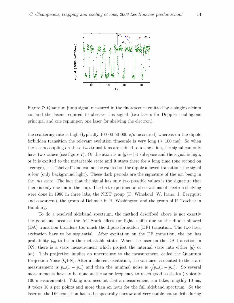
Figure 7: Quantum jump signal measured in the fluorescence emitted by a single calcium

ion and the lasers required to observe this signal (two lasers for Doppler cooling,one

principal and one repumper, one laser for shelving the electron).

the scattering rate is high (typically 10 000-50 000 c/s measured) whereas on the dipole

forbidden transition the relevant evolution timescale is very long (≥ 100 ms). So when

the lasers coupling on these two transitions are shined to a single ion, the signal can only

have two values (see figure 7). Or the atom is in |g〉− |e〉 subspace and the signal is high,

or it is excited to the metastable state and it stays there for a long time (one second on

average), it is “shelved” and can not be excited on the dipole allowed transition: the signal

is low (only background light). These dark periods are the signature of the ion being in

the |m〉 state. The fact that the signal has only two possible values is the signature that

there is only one ion in the trap. The first experimental observations of electron shelving

were done in 1986 in three labs, the NIST group (D. Wineland, W. Itano, J. Bergquist

and coworkers), the group of Dehmelt in H. Washington and the group of P. Toschek in

Hamburg.

To do a resolved sideband spectrum, the method described above is not exactly

the good one because the AC Stark effect (or light- shift) due to the dipole allowed

(DA) transition broadens too much the dipole forbidden (DF) transition. The two laser

excitation have to be sequential. After excitation on the DF transition, the ion has

probability pm to be in the metastable state. When the laser on the DA transition in

ON, there is a state measurement which project the internal state into either |g〉 or

|m〉. This projection implies an uncertainty to the measurement, called the Quantum

Projection Noise (QPN). After a coherent excitation, the variance associated to the state

measurement is pm(1 − pm) and then the minimal noise is√

pm(1 − pm). So several

measurements have to be done at the same frequency to reach good statistics (typically

100 measurements). Taking into account that a measurement run takes rougthly 10 ms,

it takes 10 s per points and more than an hour for the full sideband spectrum! So the

laser on the DF transition has to be spectrally narrow and very stable not to drift during


this spectrum by more than a step (typically 1 kHz).

3 Laser cooling of trapped ions

3.1 Doppler cooling

• If the recoil frequency ωrec = hk2L/2m≪ Γ, then the usual Doppler cooling process

works and the semi-classical treatment can be applied.

• If ωx,y,z ≪ Γ one absorption/emission cycle occurs in a time a lot shorter than the

oscillation periods, the ion velocity does not change much during one cycle and the

continuous force model explaining Doppler cooling limit can be applied.

Γgm < ωrec < ωx,y,z < Γge

≃ 1 Hz ≃ 10 kHz ≃ 1 MHz ≃ 10 MHz

• For the experiments we are interested in, it is very important that ωrec ≪ ωx,y,z as

η = kLx0 =√

ωrec/ωx,y,z.

• DA transition |g〉 → |e〉 are used for Doppler cooling whereas the DF transition

|g〉 → |m〉 are used for QI, metrology...

• Contrary to neutral atom Doppler cooling, a single direction of propagation is

enough to cool trapped ions, as long as this direction has projection on all the

symmetry axis of the trap. Nevertheless, there are several reasons that can prevent

laser cooled ions to reach the Doppler limit...

3.1.1 Excess micromotion

If bias voltage builds up in the trap, the pseudopotential center is shifted from the node

of the electric field. Then, the ion oscillates around a shifted position:

x(t) = (X cosωxt+ ǫx)(1 +qx2

cos Ωt) (54)

this gives rise to an excess contribution to the velocity which is driven by the rf field. It

can be nulled only by applying compensation voltages to side electrodes. But a diagnostic

is required to evaluate ǫx, let’s mention

1. the rf correlation technique: by a time to amplitude converter (TAC), you look for

a modulation at frequency Ω in the DA transition fluorescence. It is the method

to start with as it does not requires very cold ions. The limitation is that to have

information on excess micromotion in 3D, three directions of propagation are needed.

Some setups only offer partial information.

2. the resolved sideband spectra where the Ω band is the signature of excess micromo-

tion. To be relevant, this method must be applied to an ion already close to the

Lamb-Dicke regime.


3.1.2 Having several sidebands inside the Doppler spectrum

Even if the motional sidebands are not resolved (Γ ≫ ω), the quantum treatment of the

motion inside the laser coupling Hamiltonian can be applied. In our usual approximations

(travelling wave, low micromotion regime, Lamb-Dicke regime), but without neglecting

the micromotion, the first order expansion in η of V I is (work of Cirac, Garay, Blatt,

Parkins and Zoller in 1994)

V I =hΩL

2|e〉〈g|

(

1e−i(δt−ψ) + iη∞∑

−∞C2n

(

a†e−i(δ−ω−nΩ)t−ψ + iηae−i(δ+ω+nΩ)t−ψ)

+H.c.

)

(55)

This equation is an extension of the formulae developped for a perfect H.O, taking into

account micromotion and the C2n are the ones already met in the solution of the Mathieu

equation. They give the relative amplitude of each motional band ω + nΩ.

The bands excited when δ = −ω + nΩ leads to cooling whereas the band excited

when δ = +ω + nΩ leads to heating (even if n < 0). In the very realistic case where

Γ/2 ≃ Ω, when the laser detuning is chosen for Doppler cooling δ ≃ −Γ/2 the heating

band at −Ω + ω is excited and it works against the cooling process induced on the other

bands (the most important one being the −ω band). This extra heating process do not

prevent global cooling but it can prevent the ion to reach the Doppler limit.

When it is not the case, experiments have shown that usual Doppler cooling rules

apply. For an example, an experiment performed at the NIST group in 1995 (D. Wineland

and coworkers) with a Be+ ion (Γ/2π = 20 MHz) in a miniature rf-trap (Ω/2π = 230

MHz, ω/2π = 11.2 MHz) showed that for δ ≃ −Γ/2, the measured averaged vibrationnal

number is 0.47(5) where the expected number for the Doppler limit is 0.484. Notice that

this configuration is ideal for Doppler cooling as ω ≃ Γ/2.

What is the expected averaged vibrational number at the Doppler limit?

n =e−hω/kBTD

1 − e−hω/kBTD

=e−2ω/ΓDA

1 − e−2ω/ΓDA

(56)

In the limit where ω ≪ ΓDA/2, it takes the simple form n = ΓDA/2ω which is of the order

of 10, at the most.

Historically, the first demonstrations of laser cooling on an ion cloud were reported in

1978 (but not to the Doppler limit) for 50 Ba+ ions in a rf trap by Toschek, Dehmmelt and

coworkers and for Mg+ ions in a Penning trap by D. Wineland, Drullinger and coworkers

at NBS (now NIST) (see bibliography for references).

3.2 Resolved sideband cooling

If the effective linewidth of the transition satisfies Γe ≪ ωx,y,z, then the motional sidebands

are resolved and it is possible to tune the laser on the first red sideband (1RSB) to cool

the vibrational motion until n → 0, if no heating couterbalance this cooling. The spirit

of sideband cooling is to excite the ion on a transition where one phonon (hω) is missing


to the atomic energy transition. Once excited, the ion emits spontaneously a photon. To

reach an efficient cooling, the emitted photon must have the atomic transition energy hω0

so the system has to be already in the Lamb-Dicke regime. If not, the probability for the

photon to be emitted with energy h(ω0 − ω) is non negligeable and several absorption-

emission cycles do not result in cooling.

More precisely, the efficiency of SB cooling can be estimated in the non saturated

regime, by rate equations, assuming the system is in the LD regime and that the laser

is tuned on the 1RSB (δ = −ω). This work is due to S. Stenholm in 1986 (RMP) and

keeps coupling in the lowest order in η. It assumes that W (δ) = Γ2e/(4δ

2 + Γ2e) is the

linewidth profile without saturation, that for absorption on sideband, the relevant η is

(kL.x)x0 if we are interested in the cooling of the x-motion. But for spontaneous emission

on sidebands, the effective ηe has to take into account that only a fraction of the mean

squared wavevector project along Ox : 〈k2x〉es = α〈k2

L〉 and then η2e = α(kLx0)

2.

Let’s call R± the rate for transition from |g, n〉 to |g, n± 1〉. In the lowest order in

η, R+ results from the sum of two processes : excitation to |e, n〉 followed by relaxation

to |g, n+ 1〉 and excitation to |e, n+ 1〉 followed by relaxation to |g, n+ 1〉. This writes

R+ = W (δ)Ω2L

Γ2e

× Γeη2e(n+ 1) +W (δ − ω)

Ω2Lη

2(n+ 1)

Γ2e

× Γe (57)

=Ω2L

Γe

(

η2eW (δ) + η2W (δ − ω)

)

(n+ 1) = A+(n+ 1). (58)

As for R−, the same points lead to:

R− = W (δ)Ω2L

Γ2e

× Γeη2en+W (δ + ω)

Ω2Lη

2n

Γ2e

× Γe (59)

=Ω2L

Γe

(

η2eW (δ) + η2W (δ + ω)

)

n = A−n. (60)

From these two rates, one can calculate the time evolution of the averaged vibrational

number in the ground state 1:

dn

dt= R+(+1) +R−(−1) = A+(n+ 1) − A−n (61)

= (A+ − A−)n+ A+. (62)

Notice that for δ < 0, A− > A+. The time evolution is then

n(t) = n0e−(A−−A+)t + nf (1 − e−(A−−A+)t) (63)

with nf = 1/(A−/A+ − 1). If δ = −ω and ω2 ≫ Γ2e

A+ =Ω2LΓe

4ω2

(

η2e +

η2

4

)

and A− =Ω2L

Γeη2 (64)

1this is a simplified equation based on the linearity of the rates with n but you can do the full

calculation with each n and its probability of occupation P (n), you’ll end with the same differential

equation for n


one can see that A− ≫ A+ and the reached mean vibrational number takes the simple

form

nf ≃A+

A− =Γ2e

4ω2

(

1

4+η2e

η2

)

. (65)

The main conclusion is that for resolved sideband cooling, the final vibrational state is

described by nf which scales like (Γe/2ω)2 ≪ 1, to compare to the mean occupation

number reached by Doppler cooling nD ≃ ΓDA/2ω.

The first experiment in which the motional ground state was reached by RSBC was

performed on a single Hg+ ion, in 1989, at the NIST group (J. Bergquist, W. Itano, D.

Wineland and coworkers). The RSBCooling was using a quadrupolar electric transition,

broadened by coupling on a dipole transition with an extra laser, to make the cooling

faster.

3.3 Cooling a chain of ions

In a linear trap, if ωz < ωx, ωy, when cooled down, the ions form a chain at the node of the

electric field (the symmetry axis). More precisely if ωx,y > ωc ≃ 3N/(4√

lnN)ωz the stable

configuration is a line. When ωx,y becomes smaller than ωc there is a transition to a zig-

zag configuration and if ωx,y is further lowered, the ions move to an helicoidal structure.

In practise, for high precision spectroscopy application, the trap is operated to have a

line as a stable configuration. To reach such a configuration, the kinetic energy must be

lowered so the Coulomb repulsion can be strong enough to lead to a self organisation of

the system. For an infinite sample, it was shown a long time ago that, the phase transition

to crystals appear for

Γplasma =Q2

4πǫ0a/kBT ≤ 174 (66)

with a the mean distance between ions. When the system is finite, this criterium is mod-

ified, but still, a phase transition occurs for a given temperature that can be reached by

Doppler cooling (the order of 10-100 mK). Then the line is characterized by a nonuniform

density which means that distance between ions increase to the border of the trap and

then no Bloch theorem or other nice theorem related to periodicity can be used.

Resolved sideband cooling is also very efficient on a chain of ions but now the

relevant frequencies of oscillation in the trap are the common vibrational modes. In 1998,

the NIST group (D. Wineland and coworkers, Boulder, Colorado) managed to cool the

collective modes of motion of two Be+ (Raman transition) in an elliptical trap which is

elongated along the Ox axis. The two ions common mode were then (c.o.m for center of

mass)


c.o.mx ωcom = ωx

stretchingx ωstr =√

3ωcom

c.o.my = ωy

c.o.mz = ωz

x− y rocking =√

ω2y − ω2

x

x− z rocking =√

ω2z − ω2

x

When illuminating by a laser beam, the internal states cannot be considered inde-

pendantly because an excitation on a vibrational sideband on one ion will modify the

common vibrational state. So the states that must be considered now are of the form

|g, g, ncom〉 or |g, e, nstr〉.

For one ion, on the 1RSB along Ox, Ωnx,nx−1 = ηx√nxΩL. For two ions, excitation on the

1RSB along Ox, the effective Rabi frequency for the coupling is√

2(2nx − 1)η′

xΩL where

η′

x depends on the excited vibrational mode:

• for c.o.m, η′

x = ηx/√

2 as x′

0 = x0/√

2 for m→ 2m.

• for stretching mode, η′

x = ηx/√

2√

3 as x′

0 = x0/√

2√

3 for m → 2m and ωx →√3ωcom.

Notice that for n→ n± 1, only one atom changes its internal state:

|g, g, n〉 → |g, e, n± 1〉 or |e, g, n± 1〉

As the frequencies of the different modes are different, the RSBCooling has to act sequen-

tially on each band. For the experiment mentionned above, the results were consistent

with a thermal state with

ncom = 0.11+0.17−0.03 ⇒ n = 0 for 90%+3

−12 of time (67)

nstr = 0.01+0.08−0.01 ⇒ n = 0 for 99%+1

−7 of time (68)

the difference between the two modes can be explained by their different symmetry (it

takes an asymmetric perturbation to heat an asymmetric mode).

One could think that it is sufficient to cool the vibrational modes of interest and

ignore the other ones but if they are not cold enough, these other modes can alter the

laser coupling, to second order in η. Let’s imagine mode 2 is not cooled so down whereas

we want to excite n→ n′

on mode 1. Then one can show that the effective Rabi frequency

for this coupling is

Ωn1,n′

1

(n2) = ΩLη1√n1>e

−(η21+η2

2)/2(1 − n2η

22) (69)

So experiments are not reproductible if n2 is let to warm up.

Sharing a common vibrational mode allows to entangle internal states of several

ions by entangling their internal and external degrees of freedom. This results in one of

the most striking application of trapped ions: Creation of entangled states for Quantum

Computation gates.


4 Examples of experiments with trapped ions

4.1 Entanglement with trapped ions

4.1.1 Controlled-NOT gate with a single ion

The idea of using a trapped ion system to implement a quantum computer was suggested

by I. Cirac and P. Zoller in 1995. It initiated large efforts to realize fundamental quantum

logic gates based on entanglement. The first entanglement with trapped ion was realised

between the internal and external degree of freedom of a single Be+ ion in 1995 in the

NIST group (C. Monroe, D. Wineland and coworkers). In this experiment, the controlled

NOT gate is operated with the control qubit being the vibrational state |0〉 or |1〉 and

the target qubit being the internal state |g〉 or |e〉. So the relevant basis set contains 4

eigenstates :

|0, g〉; |0, e〉; |1, g〉; |1, e〉By laser pulses (on Raman pulses in the case of Be+) tuned on the red sideband, it is

possible to coherently couple |0, e〉 and |1, g〉 whereas on the blue sideband the coupling

is between |0, g〉 and |1, e〉. From that, one can realize the basis brick for a quantum

computer: the controlled NOT gate. It requires that the ion is first cooled in the vibra-

tional ground state with a high probability. The following sequence is the one used in the

experiment mentionned above but other sequences can be used, depending on the internal

structure of the atom.

1. the first step is a π/2 pulse on the carier (ΩLT = π/2 at δ = 0). It creates a linear

superposition of |g〉 and |e〉.

2. then, there is a 2π pulse on the blue sideband between |e〉 and an auxiliary state

|aux〉. Its effect is to modify the sign of |1, e〉 only.

3. finally, a second π/2 pulse on the carier is applied, dephased by π compared to the

first one.

init π/2 2π π/2 final

cb bsb cb’

aux-e

|g〉|0〉 → +|g〉+|e〉√2

|0〉 → +|g〉+|e〉√2

|0〉 → |g〉|0〉|e〉|0〉 → −|g〉+|e〉√

2|0〉 → −|g〉+|e〉√

2|0〉 → |e〉|0〉

|g〉|1〉 → +|g〉+|e〉√2

|1〉 → +|g〉−|e〉√2

|1〉 → |e〉|1〉|e〉|1〉 → −|g〉+|e〉√

2|1〉 → −|g〉−|e〉√

2|1〉 → |g〉|1〉

When conparing the initial and final states, one can see the truth table of the

controlled gate: When the vibrational level is |0〉, the internal state is not modified, on

the contrary, when the vibrational level is |1〉, the internal state is modified. The role of

the π/2 pulse is to build a quantum state sensitive to a modification of the sign on one

internal state.


4.1.2 Controlled-NOT gate with two ions

The idea here is that the common vibrational mode is only used to entangle states but is

not part of the truth table anymore. Here, the control qubit is ion1 whereas the target

qubit is ion2. This was first realized in the group led by R.Blatt in Innsbruck in 2003 (F.

Schmidt-Kaler and coworkers). To work, the gate has to start with the ions cooled to the

vibrational ground state.

1. the first step is a π pulse on ion1, on the 1BSB. The purpose of this step is to copy

the internal state of ion1 onto the vibrational state, it is called the SWAP operation.

2. the second step is a controlled-NOT gate like explained above, between the common

vibrational mode and the internal state of ion2.

3. the last step is a π pulse on the 1BSB, π dephased compared to the first pulse.

init π1 cnot π1 final

bsb ion2 bsb’

|g1g2〉|0〉 → |e1g2〉|1〉 → |e1e2〉|1〉 → |g1e2〉|0〉|g1e2〉|0〉 → |e1e2〉|1〉 → |e1g2〉|1〉 → |g1g2〉|0〉|e1g2〉|0〉 → |e1g2〉|0〉 → |e1g2〉|0〉 → |e1g2〉|0〉|e1e2〉|0〉 → |e1e2〉|0〉 → |e1e2〉|0〉 → |e1e2〉|0〉

One notice that the common vibrational state is not part of the truth table of the

gate, it is only a mean to entangle ions internal state. Like expected, the internal state of

ion1 controls the modification of ion2. This example of controlled gate gives you the spirit

of controlled entanglement of ions for quantum computation. Many more sophisticated

gates have been demonstrated since and now people are able to realise gates with 8 ions.

4.2 High precision metrology with entangled ions

Trapped single ions are among the best candidates for optical frequency standard as they

can be trapped and interrogated for a very long time in a very well controlled environment.

Techniques of quantum information processing can be used to increase the fidelity of the

detection. This is very useful if the clock qubit does not have an efficient cycling transition

(or its wavelength is unreachable) and/or if the shelving technique does not result in a

100% detection efficiency.

The first example of such an application is the Al+/Be+ clock developped at NIST.

Al+ is a very good candidate on the metrological point of view as it does not suffer (or far

less than usual ion) from the systematic shifts that are responsible for the finite accuracy

of other ion clocks (quadrupole shift, black body radiation shift...). But on a detection

and cooling point of view, it is a bad choice and its internal state is hard to detect with

the conventional quantum jump techniques: Be+ ion is here to play that role, the internal

state of Al+ is read on Be+ after entanglement of these two ions.


Here is the measurement sequence: it implies Al+ internal states:

|g〉 = |1S0, F = 5/2,mF = 5/2〉 (70)

|e〉 = |3P0, F = 5/2,mF = 5/2〉 τ = 21s (71)

For Be+ internal states, they are two sublevels of the ground state coupled by Raman

coupling:

| ↓〉 = |2S1/2, F = 2,mF = −2〉 (72)

| ↑〉 = |2S1/2, F = 1,mF = −1〉 (73)

1. Doppler cooling on Be+ ion, Al+ cooled by sympathetic cooling.

2. Resolved sideband cooling of the axial modes to vibrational ground state, using the

Raman coupling in Be+.

3. Preparation of Be+ in state | ↓〉.

4. Al+ is excited by the clock laser and is left in the coherent superposition α|g〉+β|e〉.

5. This internal state is maped onto the vibrational state by a π pulse on the BSB

coupling |0〉|g〉 to |1〉|aux〉.

6. The motional state information is transferred to Be+ internal state using a π pulse

on the transition |1〉| ↓〉 → |0〉| ↑〉. So finally the Al+ and Be+ are entangled

(α|g〉 + β|e〉) | ↓〉 → α|aux〉| ↑〉 + β|e〉| ↓〉 (74)

7. The internal state of Be+ is measured by the quantum jump technique which projects

its state into | ↓〉 with probability |β|2 or | ↑〉 with probability |α|2. In the first case,

the Al+ state is projected onto |e〉, in the second case, onto the manyfold (|aux〉, |g〉).

A single round has a fidelity of measurement 0.85, which is low. But by repeating

the measurement and processing some real time analysis, the fidelity reaches 0.9994. This

technique allows to reach a relative systematic uncertainty of 2, 3.10−17 on the Al+ clock

frequency measurement (at 267 nm). With the conventional optical Hg+ clock in NIST

this uncertainty is 1, 9.10−17 (at 282 nm) which represents a better precision but this

clock is a far older project than the Al+/Be+ clock so people expect the precision of this

younger project to be improved in the future. The comparison of these two clocks also

infer their stability to 2, 8.10−15/√

τ(s).

Another application of entanglement related to metrology, is the preparation of

entangled ions in a decoherence-free subspace to reach higher precision on a measurement.

This has been achieved in the Innsbruck group with two calcium ions 40Ca+ in Zeeman

sublevels of the metastable state: |D5/2,mJ〉. The purpose is to measure precisely the

electric quadrupole of level |D5/2〉 which is responsible for one of the major systematic


frequency shift on the clock transition by its coupling to electric field gradient. With a

single ion, the precision of this measurement is reduced by the fluctuations of the first

order Zeeman effect. By building the two ions Zeeman state

|ψ〉 =1√2|−5/2〉1| + 3/2〉2 + | − 1/2〉1| + 1/2〉2) , (75)

the total Zeeman number for each part of these linear combination is -1 so these two

parts are not dephased by a first order Zeeman shift (this subspace is protected from

decoherence induced by first order Zeeman effect). On the contrary, as the quadrupole

shift depends on J(J+1)−3m2J , it is negative for the first term of the linear combination

and positive for the second. So this effect induces a dephasing between these two parts

which can be measured by interferometric method (like Ramsey fringes). This method

allowed to gain an order of magnitude in the estimation of the quadrupole, compared

to the conventional method where the frequency shift is measured for different applied

electric field gradients.

4.3 Sympathetic cooling

The end of the lesson was devoted to application of sympathetic cooling, for few ions and

also for large samples. In both cases it allow, for example, to cool molecular ions and study

cold chemical reactions. Several examples of reactions are presented. It is important to

note that sympathetic cooling is very efficient to cool the translation degree of motion (to

typically 10-100 mK) even if the mass ratio and the number ratio between the two species

is very high, but it is unefficient for cooling vibration and rotation of molecular ions.

After looking at different examples of experimental realisation, the lesson concludes

on the peculiarity of the quadrupole geometry compared to the multipole one and tries

to show how different the dynamics and statistics are in both cases.


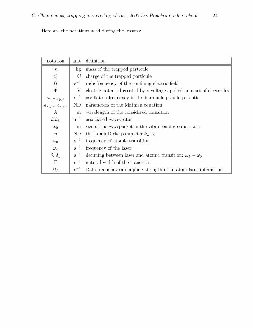
Here are the notations used during the lessons:

notation unit definition

m kg mass of the trapped particule

Q C charge of the trapped particule

Ω s−1 radiofrequency of the confining electric field

Φ V electric potential created by a voltage applied on a set of electrodes

ω, ωx,y,z s−1 oscillation frequency in the harmonic pseudo-potential

ax,y,z, qx,y,z ND parameters of the Mathieu equation

λ m wavelength of the considered transition

k,kL m−1 associated wavevector

x0 m size of the wavepacket in the vibrational ground state

η ND the Lamb-Dicke parameter kL.x0

ω0 s−1 frequency of atomic transition

ωL s−1 frequency of the laser

δ, δL s−1 detuning between laser and atomic transition: ωL − ω0

Γ s−1 natural width of the transition

ΩL s−1 Rabi frequency or coupling strength in an atom-laser interaction


Here is a short bibliography to start with. Most groups make their papers available

from their website.

1 All you want to know about radiofrequency traps

References

[1] Wolfgang Paul. Electromagnetic traps for charged and neutral particles. Rev. Mod.

Phys., 62(3):531–540, 1990. (the Nobel lecture)

[2] P. K. Gosh. Ion traps. Oxford university press, 1995.

[3] D. Gerlich. Inhomogeneous rf fields: a versatile tool for the study of processes with

slow ions. In Cheuk-Yiu Ng and Michael Baer, editors, State-selected and state-to-

state ion-molecule reaction dynamics, Part I, volume 82 of Advances in Chemical

Physics Series. John Wiley and Sons, 1992.

[4] M. Drewsen and A. Brøner. Harmonic linear paul trap: Stability diagram and effec-

tive potentials. Phys. Rev. A, 62(4):045401, 2000.

2 Laser cooling of trapped ions

[5] W. Neuhauser, M. Hohenstatt, P.E. Toschek, and H.G. Dehmelt. Optical-sideband

cooling of visible atom cloud confined in parabolic well. Phys. Rev. Lett., 41:233–236,

1978.

[6] D. J. Wineland, R. E. Drullinger, and F. L. Walls. Radiation-pressure cooling of

bound resonant absorbers. Phys. Rev. Lett., 40(25):1639–1642, 1978.

[7] D. J. Wineland and Wayne M. Itano. Laser cooling of atoms. Phys. Rev. A,

20(4):1521–1540, 1979.

[8] Wayne M. Itano and D. J. Wineland. Laser cooling of ions stored in harmonic and

penning traps. Phys. Rev. A, 25(1):35–54, 1982.

review about laser cooling of trapped ions :

[9] J. Eschner, G. Morigi, F. Schmidt-Kaler, and R. Blatt. Laser cooling of trapped ions.

J. Opt. Soc. Am. B, 20:1003, 2003.

general review about the quantum dynamics of single trapped ions:

[10] D. Leibfried, R. Blatt, C. Monroe, and D. Wineland. Quantum dynamics of single

trapped ions. Rev. Mod. Phys., 75(1):281–324, 2003.


2.1 Toward ion crystals

[11] F. Diedrich, E. Peik, J. M. Chen, W. Quint, and H. Walther. Observation of a phase

transition of stored laser-cooled ions. Phys. Rev. Lett., 59(26):2931–2934, 1987.

[12] D. J. Wineland, J. C. Bergquist, Wayne M. Itano, J. J. Bollinger, and C. H. Manney.

Atomic-ion Coulomb clusters in an ion trap. Phys. Rev. Lett., 59(26):2935–2938,

1987.

[13] M. G. Raizen, J. M. Gilligan, J. C. Bergquist, W. M. Itano, and D. J. Wineland.

Ionic crystals in a linear Paul trap. Phys. Rev. A, 45(9):6493–6501, 1992.

2.2 Resolved sideband cooling of single ion and chain of ions

[14] D. J. Wineland, Wayne M. Itano, J. C. Bergquist, and Randall G. Hulet. Laser-

cooling limits and single-ion spectroscopy. Phys. Rev. A, 36(5):2220–2232, 1987.

[15] F. Diedrich, J. C. Bergquist, Wayne M. Itano, and D. J. Wineland. Laser cooling to

the zero-point energy of motion. Phys. Rev. Lett., 62(4):403–406, 1989.

[16] B. E. King, C. S. Wood, C. J. Myatt, Q. A. Turchette, D. Leibfried, W. M. Itano,

C. Monroe, and D. J. Wineland. Cooling the collective motion of trapped ions to

initialize a quantum register. Phys. Rev. Lett., 81(7):1525–1528, 1998.

[17] H. Rohde, S. T. Gulde, C. F. Roos, P. A. Barton, D. Leibfried, J. Eschner, F. Schmidt-

Kaler, and R. Blatt. Sympathetic ground state cooling and coherent manipulation

with two-ion-crystals. J. Opt. B, 3:S34, 2001.

2.3 Cooling with quantum interference (EIT cooling)

[18] G. Morigi, J. Eschner, and C. Keitel. Ground state laser cooling using electromag-

netically induced transparency. Phys. Rev. Lett., 85(21):4458, 2000.

[19] C. Roos, D. Liebfried, A. Mundt, F. Schmidt-Kaler, J. Eschner, and R. Blatt. Ex-

perimental demonstration of ground state cooling with electromagnetically induced

transparency. Phys. Rev. Lett., 85(26):5547, 2000.

[20] G. Morigi. Cooling atomic motion with quantum interferences. Phys. Rev. A,

67:033402, 2003.


3 Entanglement and quantum logic with trapped

ions

[21] J. I. Cirac and P. Zoller. Quantum computations with cold trapped ions. Phys. Rev.

Lett., 74(20):4091–4094, 1995.

[22] C. Monroe, D. M. Meekhof, B. E. King, W. M. Itano, and D. J. Wineland. Demon-

stration of a fundamental quantum logic gate. Phys. Rev. Lett., 75(25):4714–4717,

1995.

[23] Q. A. Turchette, C. S. Wood, B. E. King, C. J. Myatt, D. Leibfried, W. M. Itano,

C. Monroe, and D. J. Wineland. Deterministic entanglement of two trapped ions.

Phys. Rev. Lett., 81(17):3631–3634, 1998.

[24] Ch. Roos, Th. Zeiger, H. Rohde, H. C. Nagerl, J. Eschner, D. Leibfried, F. Schmidt-

Kaler, and R. Blatt. Quantum state engineering on an optical transition and deco-

herence in a Paul trap. Phys. Rev. Lett., 83(23):4713–4716, 1999.

[25] D. Leibfried, E. Knill, S. Seidelin, J. Britton, R. B. Blakestad, J. Chiaverini, D. B.

Hume, W. M. Itano, J. D. Jost, C. Langer, R. Ozeri, R. Reichle, and D. J. Wineland.

Creation of a six-atom ’schrodinger cat’ state. nature, 453:4091, 2005.

[26] H. Haffner, W. Hansel, C.F. Roos, J. Benhelm, D. Chak al kar, M. Chwalla,

T. Korber, U.D. Rapola nd M. Riebe, P.O. Schmidt, C. Becher, O. Guhne, W. Dur,

and R. Blatt. Scalable multiparticule entanglement of trapped ions. nature, 438:

page 643, 2005.

[27] M. D. Barrett, J. Chiaverini, T. Schaetz, J. Britton, W. M. Itano, J. D. Jost, E. Knill,

C. Langer, D. Leibfried, R. Ozeri, and D. J. Wineland. Deterministic quantum

teleportation of atomic qubits. nature, 429:737, 2004.

[28] M. Riebe, H. Haffner, C. F. Roos, W. Hansel, J. Benhelm, G. P. T. Lancaster, T. W.

Korber, C. Becher, F. Schmidt-Kaler, D. F. V. James, and R. Blatt. Deterministic

quantum teleportation with atoms. nature, 429:734, 2004.

3.1 Using entangled states for high precision metrology

[29] D. J. Wineland, J. J. Bollinger, W. M. Itano, F. L. Moore, and D. J. Heinzen. Spin

squeezing and reduced quantum noise in spectroscopy. Phys. Rev. A, 46(11):R6797–

R6800, 1992.

[30] D. B. Hume, T. Rosenband, and D. J. Wineland. High-fidelity adaptive qubit de-

tection through repetitive quantum nondemolition measurements. Physical Review

Letters, 99(12):120502, 2007.


[31] T. Rosenband, D. B. Hume, P. O. Schmidt, C. W. Chou, A. Brusch, L. Lorini, W. H.

Oskay, R. E. Drullinger, T. M. Fortier, J. E. Stalnaker, S. A. Diddams, W. C. Swann,

N. R. Newbury, W. M. Itano, D. J. Wineland, and J. C. Bergquist. Frequency ratio of

Al+ and Hg+ single-ion optical clocks; metrology at the 17th decimal place. science,

319:1808, 2008.

[32] C.F. Roos, M. Chwalla, K. Kim, M. Riebe, and R. Blatt. ’designer atom’ for quantum

metrology. nature, 443: p316,2006.

[33] M. Chwalla, K. Kim, T. Monz, P. Schindler, M. Riebe, C.F. Roos, and R. Blatt.

Precision spectroscopy with two correlated atoms. Appl. Phys. B, 89:p483,2007.

4 Cooling of large samples and phase transition

[34] R. Blumel, J.M. Chen, E. Peik, W. Quint, W. Schleich, Y.R. Shen, and H. Walther.

Phase transition of stored laser-cooled ions. nature, 334:309, 1988.

[35] M. Drewsen, C. Brodersen, L. Hornekær, J. S. Hangst, and J. P. Schifffer. Large ion

crystals in a linear paul trap. Phys. Rev. Lett., 81(14):2878–2881, 1998.

4.1 Sympathetic cooling

[36] P. Bowe, L. Hornekær, C. Brodersen, M. Drewsen, J. S. Hangst, and J. P. Schiffer.

Sympathetic crystallization of trapped ions. Phys. Rev. Lett., 82(10):2071–2074,

1999.

[37] K. Mølhave and M. Drewsen. Formation of translationally cold MgH+ and MgD+

molecules in an ion trap. Phys. Rev. A, 62(1):011401, 2000.

[38] M. D. Barrett, B. DeMarco, T. Schaetz, V. Meyer, D. Leibfried, J. Britton, J. Chi-

averini, W. M. Itano, B. Jelenkovic, J. D. Jost, C. Langer, T. Rosenband, and D. J.

Wineland. Sympathetic cooling of 9Be+ and 24Mg+ for quantum logic. Phys. Rev.

A, 68(4):042302, 2003.

[39] B Roth, A Ostendorf, H Wenz, and S Schiller. Production of large molecular ion

crystals via sympathetic cooling by laser-cooled Ba+. J. Phys. B, 38:3673, 2005.

Trapping and cooling of ions - Accueil - CEL

Documents

Transcript of Trapping and cooling of ions - Accueil - CEL