Appalachian Coal Industry Ecosystem Appalachian Regional Commission

1-2018

Transportation Implications of Coal Transportation Implications of Coal

Mark L. Burton University of Tennessee, Knoxville

David B. Clarke University of Tennessee, Knoxville

Follow this and additional works at: https://researchrepository.wvu.edu/arc_acie

Part of the Regional Economics Commons

Recommended Citation Recommended Citation Burton, M.L., Clarke, D.B. (2018). An Economic Analysis of the Appalachian Coal Industry Ecosystem: Transportation Implications of Coal. Appalachian Regional Commission. https://www.arc.gov/wpcontent/ uploads/2018/01/CIE3-TransportationImplicationsofCoal-2.pdf

This Article is brought to you for free and open access by the Appalachian Regional Commission at The Research Repository @ WVU. It has been accepted for inclusion in Appalachian Coal Industry Ecosystem by an authorized administrator of The Research Repository @ WVU. For more information, please contact ian.harmon@mail.wvu.edu.

Regional Research InstituteWest Virginia University

Research Paper Series

An Economic Analysis of the Appalachian Coal IndustryEcosystem

Transportation Implications of Coal

Mark L. BurtonUniversity of Tennessee, Knoxville

David B. ClarkeUniversity of Tennessee, Knoxville

Date Submitted: January, 2018

Keywords: Regional Economics, Energy, Transportation, Appalachia JEL Classification: R11, O13, O18

An Economic Analysis of the Appalachian Coal Industry Ecosystem

Transportation Implications of CoalMark L. Burton*

David B. Clarke†

January, 2018

Abstract

This report describes the direct economic relationship between the coal and railroad industries in Appalachia. It finds that between 2015 and 2016, changing electric generation strategies—including accelerated coal-powered plant retirements—combined with a downturn in coal demand contributed to losses of nearly 2,000 full-time jobs and $150 million in income across Appalachia’s railroad sector.

The original version of this report is available on the Appalachian Regional Commission website Appalachian Regional Commission website.

Recommended Citation

Burton, M.L., Clarke, D.B. (2018). An Economic Analysis of the Appalachian Coal Industry Ecosystem: Transportation Implications of Coal. Appalachian Regional Commission. https://www.arc.gov/wp-content/uploads/2018/01/CIE3-TransportationImplicationsofCoal-2.pdf

*University of Tennessee-Knoxville†University of Tennessee-Knoxville

AcknowledgementsThis report was prepared for the Appalachian Regional Commission under contract PW-18673-16.

<This page blank>

An Economic Analysis of the Appalachian Coal

Industry Ecosystem

Mark L. Burton and David B. ClarkeWest Virginia University

andThe University of Tennessee

Transportation Implications of Coal

Prepared for the Appalachian Regional Commission

under contract # PW-18673-16 January 2018

1

Table of Contents List of Tables ..................................................................................................... 2

List of Figures .................................................................................................... 2

Executive Summary ............................................................................................. 3

Chapter 1: Introduction ........................................................................................ 5

Why A Freight Rail Focus? ............................................................................ 5

Goals and Organization ............................................................................... 5

Chapter 2: The Evolving Role of Rail ......................................................................... 7

Railroads as a Source of Commerce and Employment .......................................... 7

Appalachian Coal: Where It’s Mined and Where It’s Consumed ............................... 8

Appalachian Coal: How It Moves ................................................................... 10

Chapter 3: Understanding the New Normal ................................................................ 13

Chapter 4: Future Rail Access in an Era of Diminished Coal ............................................ 16

Modeling Railroad Activity Under Future Demands ............................................. 16

Future Railroad Traffic and Traffic Flows in Appalachia ...................................... 18

The Costs of Moving Surviving Traffic ............................................................. 24

Chapter 5: Policy Implications and Conclusions........................................................... 27

Key Findings ........................................................................................... 27

The Potential for Regional and State Responses ................................................ 28

Cautions, Caveats, and Closing Thoughts ........................................................ 31

Appendix A: Defining the Appalachian Rail Network ..................................................... 32

Appendix B: Analytical Methodology, Assumptions, and Parameters ................................. 34

Appendix C: An In-Depth Description of RAILNET ......................................................... 38

Appendix D: Post-Processing Cost Calculations ........................................................... 57

2

List of Tables 1. Railroad Employment in Appalachian Counties, 2015 ........................................... 7

2. Coal Production in the Eastern U.S., 2015-2016 ................................................. 8

3. Summary of Regional Waterway and Railroad Infrastructures ............................... 11

4. Modes Used for 2016 Regional Coal Delivery (Thousands of Short-Tons) ................... 12

5. Coal’s Share of Regional Waterway and Rail Traffic in 2016 ................................. 12

6. U.S. Coal Rail Car Loadings, 2013-2015 .......................................................... 15

7. RAILNET-Predicted Reductions in Ton-Miles ..................................................... 24

8. Potential Impacts on Railroad Costs and Rates ................................................. 25

List of Figures 1. Consumption of Appalachian Coal, 2016 .......................................................... 9

2. Simplified Regional Waterway and Railroad Networks ........................................ 11

3. Spot Market Prices for Central Appalachian Coal ............................................... 13

4. Aggregated Appalachian Coal Production Forecast ............................................ 14

5. Monthly U.S. Coal Rail Car Loadings .............................................................. 15

6. Modeling Process Summary ......................................................................... 16

7. RAILNET Operating Network ........................................................................ 17

8. Annual Losses to Railroad Coal Traffic Predicted by 2036 .................................... 19

9. Annual Carrier-Specific Losses to Railroad Coal Traffic Predicted by 2036 ................ 19

10. Coal Traffic Losses as a Share of Total Originating Traffic ................................... 20

11. RAILNET Distribution of Baseline (2011) Traffic ................................................ 22

12. RAILNET Distribution of Coal Scenario (2036) Traffic .......................................... 22

13. Differences Between Baseline and Coal Scenario Traffic Volumes .......................... 23

14. Estimated Surviving West Virginia Rail Traffic (2036) ......................................... 25

3

Executive Summary Recognizing the realities of a changing energy landscape, the Appalachian Regional Commission (ARC)

has commissioned a series of research initiatives that explore various aspects of Appalachian Coal

Industry Ecosystems (CIE). This report describes the goals, execution, and findings of a CIE effort

focused on rail freight access in the Appalachian Region.

For more than a century, railroads have played an important role in Appalachia’s coal industry

ecosystem. But that ecosystem is changing, and the long-run, downward trend in Appalachian coal

production implies a large and lasting reduction in coal traffic for the Region’s railroads. The recently

encountered cyclical traffic lapse provided policymakers with a glimpse as to how rail carriers may

adapt to more permanent traffic losses. Taken as a whole, this information suggests that preserving rail

freight access in Appalachia’s core may eventually become difficult.

Utilizing network modeling techniques developed at the University of Tennessee, the study team

modeled railroad network flows under baseline (2011) traffic conditions and with the diminished coal

flows predicted for 2036. Key findings include:

• Rather than unfolding evenly through time, the results suggest that the largest declines in railroad tonnage may have already been observed.

• Geographically, with only a few exceptions, any threats to rail access associated with reduced coal volumes seem to be constrained to Appalachia.

• While unwelcome, the magnitude of losses to rail access, either in the form of physical proximity or affordability, is not currently predicted to be catastrophic. However, this prediction depends pivotally on rail carriers’ abilities to garner adequate revenues from remaining freight traffic.

• Continued access to eastern ports and the global connectivity they afford depends largely on Appalachian coal’s competitiveness in international markets and the strength of those markets going forward.

The results suggest that, during 2015 and 2016, aggressive electric utility strategies (including

accelerated plant retirements), combined with a pronounced cyclical downturn in coal demand,

compressed more than a decade’s worth of reduced coal consumption and transportation into a two-

year span. Setting aside the broader effects of these events, the rapid reduction in coal-related

railroad activity eliminated roughly 2,000 full-time railroad jobs and $150 million in income from a

region that can ill-afford such disruptions.

Still, for policymakers, there are two advantages in this outcome. First, beginning in late 2016 and

continuing throughout 2017, coal production and transportation began to regain the more gradual,

long-run path predicted by the West Virginia University forecasts. Barring any additional, unanticipated

disruptions, this affords policymakers the opportunity to evaluate and implement policies that help

ensure the preservation of stable rail-freight access in the face of further declines in coal outputs.

4

As importantly, the temporal compression in reduced coal activity forced the Region’s railroads to act

with an immediacy that provides valuable information regarding future network adjustments.

Specifically, while the railroads have acted with deliberate speed, they have also avoided responses

that are irreversible. In adjusting to the 2015-16 collapse of coal demands, the railroads have not

abandoned trackage, have not razed or sold terminal facilities, and have shed unsustainable lines

through leases rather than line sales. In aggregate, these actions suggest a railroad industry that is

hesitant to permanently relinquish freight capacity.

If one accepts the long-run reduction in eastern railroad coal traffic as probable, the next question is

whether existing or foreseeable non-coal traffic will be drawn to Appalachian-inclusive rail corridors by

capacity made available through the loss of coal volumes. The analysis reported here suggests that this

will not happen. The rail routes in and through Appalachia were built to access the Region’s coal and

timber. The railroad trunk lines that first connected the American East with the nation’s interior were

built around Appalachia, much like the Interstate highways that came a century later.

The final question is—absent robust coal volumes and without a probable substitute—whether surviving

Appalachian freight traffic will generate sufficient activity to sustain the Region’s rail access. The

answer, for the moment, is a somewhat tentative probably. However, the key to this assurance is coal

volumes that do not permanently fall too far below those predicted in the above analysis. Without the

residual forecasted coal traffic, a positive outcome would be impossible.

5

Chapter 1: Introduction Two points seem irrefutable. First, mining, preparing, and transporting coal has been an integral part

of Appalachia’s economy for more than a century. Second, coal-related commerce everywhere is

changing in ways that will continue to challenge coal-dependent communities far into the future.

Recognizing these realities, the Appalachian Regional Commission (ARC) has commissioned a series of

research initiatives that explore various aspects of Appalachian Coal Industry Ecosystems (CIE). This

report describes the goals, execution, and findings of a CIE effort focused on rail freight access in the

Appalachian Region.

Why a Freight Rail Focus The Appalachian Regional Commission was organized in the mid-1960s to help the Region attain

economic parity with the nation. Early in that process, it became clear that one of the Region’s chief

disadvantages was its physical isolation. Accordingly, ARC’s earliest and most enduring strategies have

been to improve the physical mobility of both individuals and goods moving to, from, and within the

Region. Because access is key to Appalachia’s future in the global economy, protecting and improving

all transportation modes are among the Region’s foremost goals.

Continued transportation access via all transport modes is paramount, but the changes in the coal

industry ecosystem are not affecting all transport modes equally. Roadway access and motor carriage

are sustained by public policies and public-sector funding. Moreover, highway use is rarely coal-

dependent. The Region’s navigable waterways are another essential asset, and navigation traffic is

heavily dependent on the movement of coal. Still, like the roadways, navigable rivers are maintained

by the public sector. As such, private sector water carriers are, to a degree, insulated from the early

effects of economic change.

In contrast, the Region’s railroads—both its large, Class I carriers and its smaller short-lines—are almost

all privately owned. For these firms, the loss of coal and related freight traffic is resulting in

immediate financial pressures that demand near-term decisions about continued service and service-

sustaining investments. The market forces that guide railroad decision-making afford little flexibility,

sentiment, or broader community concern. In short, if Appalachia’s changing coal economy poses

threats to transportation resources, the Region’s railroad access is its most vulnerable asset.

Goals and Organization The work reported here is the third in a series of efforts recently undertaken by ARC. Motivated by

concerns for the Region’s rail networks, ARC’s senior leadership gathered a group of independent

scholars to prepare a briefing paper in January 2016 that described the emerging threat to

Appalachia’s rail freight access. This was followed by another Commission-sponsored effort (released in

6

March 2017) that evaluated the changing coal industry, the changes in the related demands for railroad

transportation, and potential public-sector strategies.1

The goal of the current initiative is to provide a level of detailed information that was not produced as

part of either earlier effort. Specifically, the analysis reported here combines long-run coal production

forecasts generated by West Virginia University with railroad network models developed at the

University of Tennessee to estimate the locations and extent of coal-related railroad traffic losses.

These predictions are then used to suggest if and where rail access may be lost altogether and how

railroad rates may be affected in areas where access is retained.

Chapter 2 provides readers with a contextual foundation. It briefly traces the rail industry’s role in the

evolution of Appalachia’s coal industry ecosystem and concludes with a discussion of the industry’s

current position. Chapter 3 outlines the rail-related CIE changes—both those that have already been

observed and those that are predicted. This chapter also describes how private sector decisions are

made regarding retaining or abandoning both services and infrastructure. The detailed information

alluded to above is provided in Chapter 4, including indications of which rail routes are most vulnerable

and how the costs of providing surviving railroad services may be affected. Finally, policy implications

and alternatives are discussed in Chapter 5. Technical appendices include details on the study data and

analytical techniques.

1 For a full discussion of these effects see, Mark Burton, “Access vs. Isolation Preserving Appalachia’s Rail Connectivity in the 21st Century: Part 2, Appalachian Regional Commission, Washington, DC, March 2017, https://www.arc.gov/images/programs/transp/RailAccessinAppalachiaPartTwoFinal.pdf

7

Chapter 2: The Evolving Role of Rail A mid-20th century railroad map of Appalachia reveals a spaghetti bowl containing thousands of miles of

main-line, branch-line, and mine-branch trackage operated by at least eight Class I carriers and dozens

of smaller regional and short-line railroads. The rail routes existed almost solely to transport coal in

every direction—east to the Tidewater for export, north for industrial users, and in every direction as a

transportation and household fuel. Not surprisingly, the nature and extent of these operations closely

mirrored business conditions in the coal industry and the changing demands of coal users. Beginning in

the post-World War II era, this activity was supplemented (and ultimately replaced by) the movement

of Appalachian steam coal to electricity-generating facilities. For the past 60 years, the fortunes of

America’s railroads, its coal producers, and its power generators have been tightly bound together.

Railroads as a Source of Commerce and Employment As with mining, technological advancements have dramatically reduced the labor requirements of

freight railroads. As recently as 1956, the Class I railroads employed over one million full-time workers.

Although freight traffic measured in ton-miles has more than tripled nationwide over the last sixty

years, by 2016, Class I employment had fallen to just 153,000.2

Railroad employment within Appalachia has followed the national trend. However, the railroads still

provide an important opportunity for regional labor. Table 1 shows the number of current (2015)

railroad employees in Appalachian counties for all railroads. Based on this accounting, roughly 10

percent of all railroad jobs are in Appalachia, and 17 percent of all Class I railroad employment is

within the Appalachian Region. Finally, like mining employment, railroad earnings are notably higher

than regional averages. For 2016, annual railroad worker compensation averaged $85,000. Thus, rail-

related employment brings approximately $2.2 billion in earnings to the Region each year.

Table 1: Railroad Employment in Appalachian Counties, 2015

State

Railroad Workers

State

Railroad Workers

Alabama 2,795 Pennsylvania 5,133 Georgia 1,868 South Carolina 331 Kentucky 2,096 Tennessee 2,624 Maryland 690 Virginia 3,842 Mississippi 473 West Virginia 2,971 North Carolina 429 ARC Region 26,009 New York 524 Non-Appalachia 240,733 Ohio 2,233 Total 266,742

Source: U.S. Railroad Retirement Board

2 See Association of American Railroads, Railroad Facts, various years.

8

Appalachian Coal: Where It’s Mined and Where It’s Consumed The March 2017 report cited above provides a more comprehensive description of coal transportation in

the eastern United States (see Section 3, page 10). However, given its importance, a portion of that

information has been updated for inclusion here.

Understanding the transportation of Appalachian coal requires three pieces of information. These

include: (1) data describing where domestic coal is mined, (2) similar information detailing where and

for what purposes coal is consumed (or exported), and (3) depictions (including cost and availability) of

the transportation alternatives for moving coal from source to consumption.

Table 2 summarizes eastern production for 2015 and 2016.3 Roughly one-quarter of U.S.-produced coal

was mined in Appalachia, while 13.5 percent was produced in the Illinois basin. Of the coal-producing

Appalachian states, West Virginia was dominant, producing 11.0 percent of the national output.

Table 2: Coal Production in the Eastern U.S., 2015-2016

2016 (Thousands

of Short Tons)

2016 Percent of U.S Total

2015 n (Thousands

of Short Tons)

Percentage Change

Alabama 9,643 1.3% 13,191 -26.9% Illinois 43,422 6.0% 56,101 -22.6% Indiana 28,767 3.9% 34,295 -16.1% Kentucky (East) 16,772 2.3% 28,101 -40.3% Kentucky (West) 26,096 3.6% 33,324 -21.7% Maryland 1,616 0.2% 1,922 -15.9% Mississippi 2,870 0.4% 3,143 -8.7% Ohio 12,564 1.7% 17,041 -26.3% Pennsylvania Total 45,720 6.3% 50,031 -8.6% Tennessee 644 0.1% 897 -28.2% Virginia 12,910 1.8% 13,914 -7.2% West Virginia (Northern) 43,524 6.0% 47,785 -8.9% West Virginia (Southern) 36,233 5.0% 47,848 -24.3% East of the Mississippi River 280,781 38.5% 347,593 -19.2% Appalachia Total 179,626 24.7% 220,730 -18.6% Illinois Basin 98,285 13.5% 123,720 -20.6% U.S. Total 728,364 100.0% 896,941 -18.8%

Source: Energy Information Administration

3 The current analysis focuses on production and consumption in states east of the Mississippi River unless explicitly noted otherwise.

9

In a typical year within the U.S., roughly 90 percent of all coal mined is consumed domestically, with

only 10 percent going to export. However, the characteristics and location of Appalachian coal make it

particularly attractive in broader global markets, and so export coal routinely accounts for 20-25

percent of the Region’s annual output. As the remainder of the current report highlights, the

distinction between Appalachian coal used in domestic electricity production and coal mined for export

has important implications for eastern railroads and the Region’s continued access to rail freight

service.

Of the 80 percent of Appalachian coal that is not exported, nearly all of it is burned as steam coal

within or near the Region. Figure 1 depicts coal shipments from Appalachian origins and the volume of

western and Illinois basin coal consumed by the receiving states.

Figure 1: Consumption of Appalachian Coal, 2016

Source: Energy Information Administration

10

Appalachian Coal: How It’s Moved Much of the Region’s coal is consumed relatively close to where it is mined and nearly all domestic

consumption takes place east of the Mississippi River. When distances are sufficiently short (less than

100 miles) and volumes are small, coal is sometimes moved by truck. When volumes are large and

inland navigation is feasible, coal moves by barge. Most often, however, coal moves by rail in unit

trains that often operate directly between “prep” plants and electric generating facilities or, in the

case of exports, deep-draft ports.

Both Kentucky and West Virginia have state-designated coal-haul roadway systems designed to

accommodate loaded coal trucks. In addition to these systems, the general consensus is that coal truck

travel is both possible and efficient throughout the coal-producing region wherever there are roadways

of any form. Both barge and railroad transport are different.

Private sector barge owners and towing companies operate on navigable waterways as determined by

the U.S. Coast Guard on a system that is designed, constructed, and maintained by the U.S. Army Corps

of Engineers (Corps). On most reaches of these waterways, maintaining adequate water depth depends

on establishing navigation pools created by dams that can be transited through navigation locks.4 With

very few exceptions, railroad infrastructure is privately owned by rail carriers who create, maintain,

and operate freight rail systems. A thumbnail sketch of mainline railroad trackage and main-stem

waterway system components are provided in Figure 2. The extent of these systems within the Region

is summarized in Table 3.

Table 4 provides a summary of the freight transportation modes used to deliver coal to final

destination states in 2016. Table 5 reverses the analytical lens and depicts the importance of coal

traffic as a share of overall 2016 freight activity for both rail and barge. Together, these data make

clear the rigid interdependence that has historically existed between coal production and freight

transportation. Focusing on West Virginia, Kentucky, Pennsylvania, and Ohio, 87.3 percent of all

regional coal shipments were delivered by rail or barge in 2016. Alternatively, coal traffic accounted

for 47.3 percent of all locked tonnage on the Ohio River main stem and 68.3 of all rail shipments

originating in these four states in 2016. At least historically, without the ability to move coal to where

it is consumed, the Region’s coal reserves would have been of far less value; without the need to move

coal, much of the Region’s transportation infrastructure would have been unnecessary.

4 Only two major waterway segments are devoid of locks and dams. These are the Missouri River below the head of navigation near Council Bluffs, Iowa to its confluence with the Mississippi and the lower Mississippi River for its entirety below St. Louis.

11

Figure 2: Simplified Regional Waterway and Railroad Networks

Source: Center for Transportation Research

Table 3: Summary of Regional Waterway and Railroad Infrastructures

Railroad Network Waterway Network

Primary Class I Carriers CSXT, NS Mainstem Ohio Miles 436 Total Freight RR Miles 16,970 Navigable Tributary Miles 768 Number of Short-Line Carriers 83 Mainstem Ohio Locks 12 Total Regional Short-Line Miles 5,459 Navigable Tributary Locks 33 Holding Co. Short-Lines 35 Holding Co. Short-Line Miles 3,475

Source: Center for Transportation Research

12

Table 4: Modes Used for 2016 Regional Coal Delivery (Thousands of Short-Tons)

State Rail Barge Truck Other Total

Domestic Export Total Alabama 671 1,962 1,077 3,710 6,329 10,039 Illinois 13,632 17,304 3,054 6,071 40,060 6,250 46,311 Indiana 24,112 2,719 2,498 19 29,348 172 29,520 Kentucky (East) 11,410 1,409 1,413 70 14,302 1,255 15,557 Kentucky (West) 8,574 12,707 4,439 25,720 97 25,817 Maryland 22 10 1,518 1,550 209 1,759 Mississippi 3,053 3,053 3,053 Ohio 567 14,830 3,079 18,476 137 18,613 Pennsylvania (Anthracite) 19 166 185 401 586 Pennsylvania (Bituminous) 23,393 6,939 4,113 2,026 36,471 5,607 42,077 Tennessee 618 3 17 638 638 Virginia 4,375 1,790 2,803 252 9,220 5,004 14,223 West Virginia (Northern) 4,267 19,438 150 5,010 28,864 9,681 38,546 West Virginia (Southern) 16,071 7,597 1,881 1 25,549 14,387 39,936 STUDY REGION TOTAL 107,728 86,709 29,261 13,448 237,146 49,528 286,674

Source: Energy Information Administration

Table 5: Coal’s Share of Regional Waterway and Rail Traffic in 2016

Railroad Origin State

Loaded Carloads -

Coal

Loaded Carloads -

ALL

Coal Percentage

of Total Ohio River Lock

and Dam

2016 Coal Traffic Tons

(X1K)

2016 Total Traffic

Tons (X1K)

Coal Percentage

of Total Alabama 54,483 518,718 10.5% Ohio 52 13,771 70,718 19.47% Kentucky 258,996 636,346 40.7% Ohio 53 8,171 63,695 12.83% Ohio 85,412 1,211,763 7.0% Belleville 25,487 40,485 62.95% Pennsylvania 255,372 1,089,106 23.4% Cannelton 25,510 52,367 48.71% Virginia 126,038 523,994 24.1% Meldahl 15,538 37,549 41.38% West Virginia 549,538 690,684 79.6% Dashields 7,580 12,135 62.47% ARC TOTAL 1,329,839 4,670,611 28.5% Emsworth 7,576 10,979 69.01% Illinois 295,001 4,935,567 6.0% Greenup 13,393 35,584 37.64% Indiana 170,060 750,285 22.7% Hannibal 26,578 39,562 67.18% Regional Total 1,794,900 10,356,463 17.3% Myers 15,454 47,765 32.36% US Total 5,352,604 32,335,465 16.6% Markland 14,167 39,249 36.10%

McAlpine 25,118 53,269 47.15% Montgomery 7,119 12,343 57.68% Newburgh 28,712 58,871 48.77% New Cumberland 14,253 23,953 59.51% Pike Island 15,571 26,158 59.53% Racine 28,225 43,345 65.12% Robert Byrd 12,703 30,498 41.65% Smithland 17,180 55,725 30.83% Willow Island 24,240 37,331 64.93%

Ohio River Total 346,347 791,582 43.75% Source: Association of American Railroads, U.S. Army Corps of Engineers

13

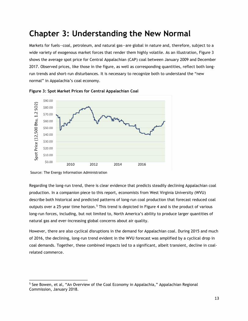
Chapter 3: Understanding the New Normal Markets for fuels—coal, petroleum, and natural gas—are global in nature and, therefore, subject to a

wide variety of exogenous market forces that render them highly volatile. As an illustration, Figure 3

shows the average spot price for Central Appalachian (CAP) coal between January 2009 and December

2017. Observed prices, like those in the figure, as well as corresponding quantities, reflect both long-

run trends and short-run disturbances. It is necessary to recognize both to understand the “new

normal” in Appalachia’s coal economy.

Figure 3: Spot Market Prices for Central Appalachian Coal

Source: The Energy Information Administration

Regarding the long-run trend, there is clear evidence that predicts steadily declining Appalachian coal

production. In a companion piece to this report, economists from West Virginia University (WVU)

describe both historical and predicted patterns of long-run coal production that forecast reduced coal

outputs over a 25-year time horizon.5 This trend is depicted in Figure 4 and is the product of various

long-run forces, including, but not limited to, North America’s ability to produce larger quantities of

natural gas and ever-increasing global concerns about air quality.

However, there are also cyclical disruptions in the demand for Appalachian coal. During 2015 and much

of 2016, the declining, long-run trend evident in the WVU forecast was amplified by a cyclical drop in

coal demands. Together, these combined impacts led to a significant, albeit transient, decline in coal-

related commerce.

5 See Bowen, et al, “An Overview of the Coal Economy in Appalachia,” Appalachian Regional Commission, January 2018.

14

Figure 4: Aggregated Appalachian Coal Production Forecast

Source: West Virginia University Forecast

Figure 5 illustrates U.S. railroad coal car-loadings from 2014 forward. Table 6 provides 2013-2015 coal

traffic data for individual carriers. These data underscore the rapid and pronounced 2015-2016 drop in

railroad coal traffic, particularly in the eastern U.S. In response, Appalachia’s railroads undertook a

variety of actions. Norfolk Southern temporarily discontinued service over two routes in West Virginia

and Ohio; leased a 300-mile secondary mainline route and a 44-mile North Carolina branch-line a to a

short-line holding company; closed its coal terminal in Ashtabula, Ohio; consolidated its division-level

operations at Bluefield and Roanoke, Virginia; and closed its yard operations in Knoxville.

CSX was as equally aggressive in its response. It closed shop facilities in Erwin, Tennessee and Corbin,

Kentucky; ceased yard operations at Russell, Kentucky; temporarily curtailed operations on portions of

its route between Russell, Kentucky and Spartanburg, South Carolina; downgraded its route between

Cincinnati and north Georgia; and ended division operations at Huntington, West Virginia.

In total, the actions noted above led to the elimination of roughly 2,000 direct, highly-compensated

jobs in Appalachia, losses that were particularly difficult for the hardest hit communities. Further,

from a policy perspective, the retrenchments signaled potential additional cuts and the possible loss of

rail network access. However, on a forward-looking basis there are, at least, three positive factors.

First, very few of the facility closures have been followed by actions that are permanent. No buildings

have been razed and no track has been abandoned. Second, in some areas where service had been

suspended, it has been restored, at least nominally. Finally, most of the actions described above were

taken in late 2015 or the first half of 2016. At present, planners for both CSX and Norfolk Southern

have indicated that further coal-related system rationalizations are not pending.

15

In the last months of 2016 and through most of 2017, the cyclical factors that brought such disarray to

U.S. coal producers have largely subsided, and coal production has inched toward recovery, but only to

the point of rejoining the WVU-predicted long-run decline.

Figure 5: Monthly U.S. Coal Rail Car Loadings

Source: The Association of American Railroads

Table 6: U.S. Coal Rail Car Loadings, 2013-2015

2013 2014 2015

Peak to Low Percent Change

U.S. Total 5,951,982 6,110,053 5,441,934 -10.9% Eastern Railroads 2,208,515 2,258,236 1,866,615 -17.3% Western Railroads 3,743,467 3,851,817 3,575,319 -7.2% CSXT 996,540 1,009,831 810,077 -19.8% Norfolk Southern 1,029,218 971,906 796,991 -22.6% Canadian National (U.S) 182,757 276,499 259,547 -6.1% BNSF 2,209,522 2,258,902 2,276,715 0.8% Kansas City Southern 2,181 2,211 7,767 251.3% Canadian Pacific (U.S.) ----- 982 3,203 226.2% Union Pacific 1,531,764 1,589,722 1,287,634 -19.0%

Source: The Association of American Railroads

16

Chapter 4: Future Rail Access in an Era of Diminished Coal Railroads continue to play an important role in Appalachia’s coal industry ecosystem, but that

ecosystem is changing. The long-run, downward trend in regional coal production implies a large and

lasting reduction in coal traffic for the Region’s railroads and the recently encountered cyclical traffic

lapse provides policymakers with a glimpse of how rail carriers may adapt to more permanent traffic

losses. Taken as a whole, this information suggests that preserving rail freight access throughout

Appalachia may eventually become difficult.

What remains in this section is an attempt to lend precision to this concern—to predict where traffic

losses are likely to be greatest, to explore whether railroads have other uses for resulting excess

regional capacity, to identify the railroad routes that are most vulnerable, and to estimate how

diminished railroad activity will affect the costs of moving the non-coal traffic that remains. The

remainder of this section briefly describes how the study team worked to address these issues, then

presents the results of these efforts.

Modeling Railroad Activity Under Future Demands In terms of evaluating what will happen to Appalachia’s rail access in a post-coal era, history is of little

help. The Region’s railroads were built to transport coal. Even during periods of prolonged slack

demand, coal producers and the Region’s coal-hauling railroads assumed that demands would rebound,

and traffic would return. For 100 years, they were right.

Absent a historical record with which to make predictions, the next best choice is to model potential

outcomes based on known physical and economic relationships and to simulate how substantially lower

coal traffic volumes will affect railroad behaviors. That modeling process involves several specific

steps. These are summarized in Figure 6, briefly discussed in the text that follows, and described in

detail in the report’s appendices.

Figure 6: Modeling Process Summary

17

To model railroad traffic flows, the study team used RAILNET, a GIS-based optimization model

developed at the University of Tennessee. Given a specified set of transportation demands, RAILNET

routes railroad traffic over the railroad network in a way that simulates the profit-maximizing behavior

of the Region’s railroads. This is far more realistic than similar models that minimize transit distances

or transit times. In the current application, the network, pictured in Figure 7, is confined to the Region

east of the Mississippi River and includes both Class I railroad trackage and relevant short-line

facilities.

Baseline traffic data were developed through the use of the Surface Transportation Board’s 2011

Carload Waybill Sample (CWS). 2011 was picked as the baseline year because it was the year in which

aggregate railroad industry coal revenues peaked and the last year in which coal volumes were near

their historic highs.6

Figure 7: RAILNET Operating Network

Source: Center for Transportation Research

The same 2011 baseline data were used to create the scenario dataset. The study team did not

attempt to forecast future traffic volumes for non-coal commodities. For coal movements originating in

the eastern United States, the coal data were adjusted to reflect the WVU-predicted 2036 values as

described above. Importantly, the rail traffic to, from, and within the study region includes coal mined

6 Industry-wide, railroad coal volumes peaked in 2007. See, Association of American Railroads, Annual Statistics of Class I Railroads, 1978 – 2015.

18

in regions outside Appalachia (e.g., the Illinois basin or the Powder River basin). Based on EIA

production forecasts, we assumed that production in those non-Appalachian regions would remain

constant over the 20-year time horizon.7

Future Railroad Traffic and Traffic Flows in Appalachia The results of both the data preparation and the coal scenario simulations suggest that preserving rail

freight access in Appalachia’s core may be difficult. These findings underscore the dominance of coal

traffic, the grave magnitude of the long-run predicted traffic declines, and the low probability that

unneeded capacity on most coal-dominated routes will be absorbed by network traffic currently

traversing alternative routings.

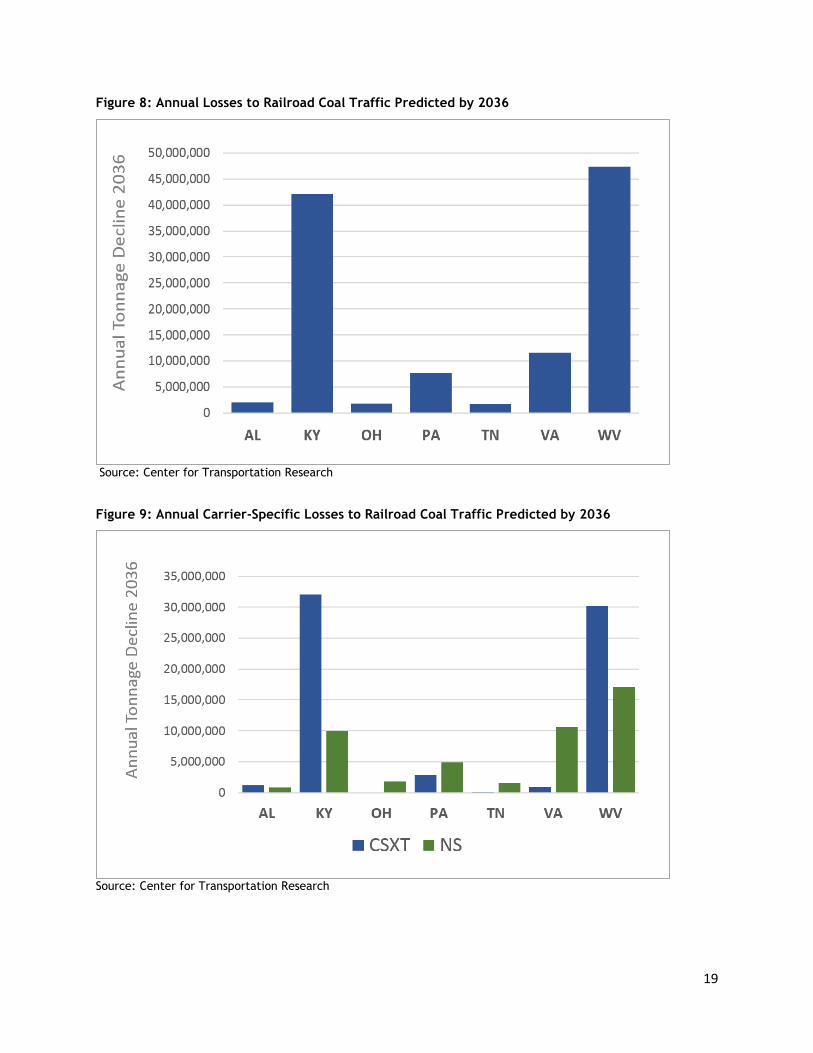
Lessons from the Scenario Data Even before the RAILNET simulations, the scenario data provided useful insights.8 Figure 8 illustrates

the total, state-specific coal traffic reductions predicted when 2011 coal production totals are

replaced with the forecasted 2036 values. The estimated traffic losses are located in exactly the same

places where early coal traffic declines have been most observable—eastern Kentucky and southern

West Virginia.

Figure 9 further decomposes the predicted losses in 2036 traffic volumes between Norfolk Southern and

CSX. In total, predicted traffic losses are 67.5 million tons for CSX compared to 46.9 million tons for

Norfolk Southern, signifying that both railroads will continue to be significantly impacted. However,

the geographic pattern varies between the two railroads. In the case of CSX, volume declines are

heavily concentrated in eastern Kentucky and southern West Virginia. While NS also will see significant

declines in these regions, its overall coal traffic losses are more evenly distributed across the seven

states where it currently originates coal movements.

The final finding attributable to the coal scenario data development is contained in Figure 10, which

depicts the predicted 2036 coal losses as a share of current originating traffic for each railroad within

each state. While neither this figure nor the data it depicts include terminating regional traffic or pass-

through network use, it is nonetheless clear that at its predicted levels, declining coal traffic will

dramatically affect the economics of providing freight rail service to the Region.

7 See U.S. Department of Energy, Energy Information Administration, Annual Energy Outlook: 2017, Supplemental Tables, “Coal Supply, Disposition, and Prices,” https://www.eia.gov/outlooks/aeo/data/browser/#/?id=15-AEO2017&cases=ref2017&sourcekey=0 8 Reporting in this section is constrained by the reliance on the Carload Waybill Sample and a need to protect both shipper and carrier confidentiality.

19

Figure 8: Annual Losses to Railroad Coal Traffic Predicted by 2036

Source: Center for Transportation Research

Figure 9: Annual Carrier-Specific Losses to Railroad Coal Traffic Predicted by 2036

Source: Center for Transportation Research

20

Figure 10 – Coal Traffic Losses as a Share of Total Originating Traffic

Source: Center for Transportation Research

The RAILNET Simulation Results The goal of the simulations was to provide stakeholders with useful information about the specific

effects of reduced coal reliance on the demand for rail transportation and the railroad infrastructure

that supports it. The simulations do that. Baseline estimates of link-specific traffic volumes

approximate the observed distribution of railroad traffic in the southeastern U.S. in 2011. The traffic

flows predicted under forecasted 2036 coal volumes correlate well with the observed effects of already

declining coal volumes and provide valuable insights into future outcomes.

Figure 11 depicts the RAILNET-generated, link-specific railroad flows, based on actual shipment origins,

destinations, and transported tonnages. Moreover, while this figure does not reflect values for

individual commodities, commodity-specific tallies are one of many available model outputs. The units

are gross tons, including empty cars, on each link.

Figures 12 and 13 depict rail traffic in the eastern U.S. based on forecasted 2036 Appalachian coal

volumes.9 Figure 12 illustrates total forecasted regional tonnage and Figure 13 captures the difference

between the coal scenario traffic and traffic under the 2011 baseline conditions. As above, units are

gross tons including empties.

There are several important results. First, as expected, the coal-producing regions—particularly West

Virginia and eastern Kentucky—experience the largest impact on predicted infrastructure use. As

9 As described in Section above, the analysis changes only Appalachian coal volumes. All other (coal and non-coal) traffic volumes are at 2011 levels.

21

noted, these regions originate little else other than coal. Further, the model results suggest that

diversions from other routes will not absorb newly available capacity on these coal-dominated route

segments. Instead, the coal routes serving central Appalachia seem segregated from other rail network

flows. This isolation leads to a second observation: With the exception of coal routes to export

locations, the predicted infrastructure impacts of reduced coal reliance are concentrated in the coal-

producing areas.

Together, the three figures highlight the importance of export coal volumes to the Region’s rail

carriers and suggest that the two mainline routes between southern West Virginia and Virginia’s deep

draft ports may be vulnerable. However, this conclusion may be attributable, at least in part, to the

forecasts’ inability to distinguish between steam coal and metallurgical coal, the latter of which is

mined specifically for export. By necessity, the WVU forecasts used here consider coal produced within

a state or within a substate region to be homogeneous. Though unavoidable, the resulting ambiguities

introduce uncertainty in interpreting the results presented here.

The results summarized in Figures 11, 12, and 13 suggest that specific routes may face traffic shortages

that threaten their viability. Interestingly, many of these seemingly vulnerable routes have already lost

traffic and undergone a change in status. This would seem to validate the model’s performance. For

example, the results predict the impact of reduced coal volumes on the CSX route between Russell,

Kentucky and the Carolinas. As noted above, this has occurred, with CSX responding by reducing the

FRA track class on some segments, suspending service on other portions of the route, and closing shop

facilities at Erwin, Tennessee. Similarly, the model predicts traffic losses for the CSX route between

Cincinnati and northern Georgia. Again, this happened, with the carrier reducing track to Class 2 and

closing locomotive maintenance facilities at Corbin, Kentucky. Loosely applied, the model output

predicts approximately 150 miles of heavy-haul trackage will be subject to abandonment or sale and

that roughly 1,200 route-miles will eventually be downgraded in terms of capacity. Much of this has

already been observed.

22

Figure 11: RAILNET Distribution of Baseline (2011) Traffic

Source: Center for Transportation Research

Figure 12: RAILNET Distribution of Coal Scenario (2036) Traffic

Source: Center for Transportation Research

23

Figure 13: Differences Between Baseline and Coal Scenario Traffic Volumes

Source: Center for Transportation Research

The predicted impacts to rail route segments are largely confined to central Appalachia and are shared

roughly equally by CSX and Norfolk Southern. Still, these two dominant eastern railroads are not the

only affected carriers. Other regional carriers also suffer traffic losses. Table 7 provides carrier-specific

predictions of losses to gross railroad ton-miles that reflect 2036 coal flows.10 Readers should bear in

mind that (1) these are predicted, not actual changes, (2) changes are measured in gross ton-miles,

10 The model also predicts a small number of net traffic gains. However, because these outcomes are not yet validated, Table 14 does not include them.

24

and (3) while the vast majority of traffic changes reflect lost coal movements, some link-specific

traffic changes may be affected by alternative routes for non-coal traffic.

Table 7: RAILNET-Predicted Reductions in Ton-Miles

Carrier

Increases in Gross Link Ton-Miles (Millions)

Decreases in Gross Link Ton-Miles (Millions)

Net Change in Gross Link Ton-Miles (Millions)

CSXT 3,824 34,554 -30,731 Norfolk Southern 3,157 30,529 -27,372 BNSF 949 9,348 -8,399 Florida East Coast 580 -580 Other Railroads 824 6,285 -5,450 TOTAL 8,754 81,296 -72,531

Source: Center for Transportation Research

The Costs of Moving Surviving Traffic Further reductions in coal traffic will clearly impact the role and profitability of regional rail

operations. However, not all coal traffic will be lost, and non-coal commodities also move by rail to

and from Appalachian communities. Therefore, it is important to anticipate how lost coal traffic may

affect the underlying costs and rates for moving the surviving coal and non-coal rail traffic. To

illustrate, estimated non-coal and surviving coal rail traffic for West Virginia in 2036 is summarized in

Figure 14. Presumably, the demand for this traffic will remain, even as other coal traffic declines.

The cost that railroads incur to move a specific shipment depends heavily on how much other traffic is

using the same routes required by the subject freight. In most cases, railroads exhibit what economists

refer to as economies of density, in which individual shipment costs are lower when there is more

(rather than less) overall traffic on route segments. It follows that the costs for moving the surviving

coal and non-coal rail shipments to and from Appalachia will increase as coal traffic continues to

decline.

As more fully explained in Appendix C, the RAILNET modeling platform used to estimate the traffic

losses described above depends on cost parameters for different commodities and differing traffic

volumes. Appendix D describes how these results were also used to estimate likely changes in unit costs

attributable to diminished coal traffic. The results of these calculations are provided in Table 8.

25

Figure 14: Estimated Surviving West Virginia Rail Traffic (2036)

Source: Center for Transportation Research, Association of American Railroads

Table 8: Potential Impacts on Railroad Costs and Rates11

Condition

Average Total Cost Per Ton-

Mile

Hypothetical Ton-Mile

Rate

Hypothetical Rate per

Ton

Hypothetical Rate per Carload)

Baseline $0.0263 $0.045 $24.00 $1,920 Short-Run $0.0752 $0.114 $68.40 $5,472 Long-Run $0.0337 $0.051 $30.72 $2,458

Source: Center for Transportation Research

Again, the full derivation of the values in Table 8 is provided in Appendix D. However, there are two

important elements to discuss here. First, the table contains both short-run and long-run cost

implications. Railroads design, modify, and maintain infrastructure based on expected use. Most of the

potentially-affected regional trackage is currently built and maintained to sustain high-density, coal-

dominated traffic. In the short-run, it is impossible to fully reduce the capacity of this infrastructure,

even if it is only lightly used. Thus, the short-run cost effects of the lost traffic are substantial. In the

11 The conversion of ton-mile rates to rates per ton and per carload are based on a hypothetical trip distance of 600 miles and a hypothetical loading weight of 80 tons per carload.

26

longer-run, however, carriers can do a great deal to reduce capacity so that the infrastructure is

consistent with lower traffic volumes. Thus, the long-run effect of reduced traffic on the costs of

continuing service for surviving traffic are not nearly as severe.

Next, the existence of common costs necessarily drives a wedge between unit costs and railroad rates.

However, there is nothing that guarantees surviving coal traffic or the demands for transporting non-

coal traffic will sustain the roughly 25 percent long-run rate increases projected in Table 8. If these

markets cannot afford these rates, then there is a chance that additional traffic will disappear or be

diverted to an alternative transport mode. This possibility makes conclusions regarding the future

viability of regional rail access more fragile than they first appear.

27

Chapter 5: Policy Implications and Conclusions This report summarizes the findings of a year-long study of the relationship between freight railroads

and Appalachia’s coal industry ecosystem. Based on already observed reductions in coal production and

production forecasts produced by West Virginia University, the analysis attempts to anticipate the

effects on the Region’s railroads over a 25-year time horizon. The results presented here are

preliminary and can be improved upon. Nonetheless, the findings hint at possible policy challenges and

opportunities. In this final section, we enumerate these and close with a discussion of potential public-

sector responses.

Key Findings The analysis has generated four key findings. These include:

1. Rather than unfolding evenly through time, the results developed here suggest that the largest declines in railroad tonnage may have already been observed.

Comparing the data projections summarized in Section 3 to the coal traffic volumes actually observed

between 2011 and 2016, it seems that much of the total forecasted decline in coal production, spread

evenly over the 2011-2036 forecast period, has actually been observed within the forecast period’s

early years. This outcome is consistent with an electric utility strategy where coal-fired generating

capacity is retired as early as possible. Thus, policymakers may have already observed much (if not the

majority) of coal traffic declines predicted over the 25-year time horizon.

2. Geographically, with only a few exceptions, any threats to rail access associated with reduced coal volumes seem to be constrained to Appalachia.

The evidence described above suggests that the ongoing and future traffic impacts attributable to

reduced coal reliance are (and will continue to be) largely constrained to Appalachia. The implication

is that the coal routes highlighted in Figure 13 exist in relative isolation from other railroad network

activities. It follows that diminished coal volumes will continue to threaten freight rail access in

Appalachia’s coal producing regions, but that this threat is not likely to spread to other segments of

the eastern U.S. Thus, discussions that compare current challenges to the broader eastern rail network

collapse barely avoided during the 1970s are without foundation. Any railroad problems associated with

declining coal reliance are likely local or regional and any policy responses to the challenges associated

with reduced rail network access will likely need to originate at the same local or regional levels.

28

3. While unwelcome and detrimental, the magnitude of losses to rail access, either in the form of physical proximity or affordability, is not currently predicted to be catastrophic. However, this prediction is somewhat fragile and depends on carriers’ abilities to garner adequate revenues from remaining freight traffic.

Generally, results do not point to a wholesale, widespread loss of rail access for the Region. However,

the same results do suggest that railroad rates for remaining coal traffic and for other non-coal

commodities will face substantial upward pressure. Specifically, the analysis identifies roughly 150

miles of Class I, mainline trackage that are highly vulnerable to sale or abandonment. The results also

point to roughly 1,200 route-miles that are likely candidates to be downgraded or, perhaps, leased to a

short-line. As importantly, the same results suggest that, even after infrastructure adjustments, Class I

carriers will need to increase rates for surviving coal and non-coal rail traffic by more than 25 percent

if the remaining traffic will sustain such increases.

4. Continued access to eastern ports and the global connectivity they afford depends largely on Appalachian coal’s competitiveness in international markets and the strength of those markets going forward.

Finally, and to reiterate, the extent of predicted reduced coal traffic between Appalachia and eastern

deep-draft ports (Norfolk, Hampton Roads, and Baltimore) depends almost exclusively on the demands

for coal exports. While many factors can influence these volumes, changes in U.S. trade policies

certainly can affect coal exports. Any modification of trade policy that diminishes the competitiveness

of Appalachian coal in global markets is also likely to further strain rail access between Appalachia and

East Coast ports.

The Potential for Regional and State Responses The results suggest that aggressive electric utility strategies, combined with a pronounced cyclical

downturn, compressed more than a decade’s worth of reduced coal consumption and transportation

demand into a four- or five-year span. Setting aside the psychological effects of this collapse, the rapid

reduction in coal-related railroad activity ripped roughly 2,000 full-time jobs and $150 million in

incomes from a region that can ill-afford such disruptions.

However, as perverse as it may seem, there are at least two advantages for policymakers in this

compressed outcome. First, beginning in late 2016 and continuing throughout 2017, coal production

and transportation began to regain the more gradual, long-run path predicted by the West Virginia

University forecasts. Barring any additional, unanticipated disruptions, this course affords policymakers

a little time to evaluate and implement policies that, as much as possible, ensure the preservation of

stable rail-freight access in the face of further declines in coal outputs.

29

Second, and just as important, the temporal compression in reduced coal activity forced the Region’s

railroads to act with an immediacy that provides valuable information regarding future network

adjustments. Specifically, while the railroads have acted with deliberate speed, they have also avoided

responses that are irreversible. In adjusting to the 2015-16 collapse of coal demands, the railroads

have not abandoned trackage, have not razed or sold terminal facilities, and have shed unsustainable

lines through leases rather than line sales. In aggregate, these actions suggest a railroad industry that

is hesitant to permanently relinquish freight capacity.

The previously referenced March 2017 ARC report provides an extensive discussion of steps that states

can take to help ensure stable rail-freight access. These activities are summarized below.

State-Level Freight Planning The most recent federal surface transportation bill, the Fixing America’s Surface Transportation (FAST)

Act continues to require that states develop statewide rail plans and that these plans be approved by

the U.S. Secretary of Transportation.12 In this light, every state should have available basic information

describing the nature and extent of railroad infrastructure, carrier operations, and traffic composition.

In addition to collecting and updating this information, states may wish to include freight plan

elements that:

• Preserve the railroad infrastructure footprint if at all possible;

• Support quick (if not automatic) state responses to potential abandonments;

• Create or, at least, identify potential sources of funding; and

• Integrate rail planning as fully as possible into broader statewide freight planning and plans for

economic development.

Experience shows that, once lost, the railroad “footprint” is difficult (or often impossible) to recreate.

Moreover, while retaining rights-of-way is essential to rail capacity preservation, the ability to restore

service to an inactive route may also depend on the presence and condition of the infrastructure on

that right-of-way. This is particularly true of tunnels, bridges, and other high-dollar infrastructure

components. North Carolina’s program for retaining abandoned trackage is exemplary in this regard.

It is also important that states be prepared to act quickly in the face of potential abandonments.

Federal reform legislation of the 1970s and 1980s included provisions that diminish the duration of

abandonment proceedings. Moreover, railroad owners are not generally compelled to discuss system

rationalization plans prior to executing them. Thus, it is easy for both on-line communities and state

12 See 49 U.S. Code § 22702 as amended by Pub. L. 114–94, div. A, title XI, § 11315(a)(1), Dec. 4, 2015, 129 Stat. 1674.)

30

authorities to be surprised by proposed abandonments. However, the same reform legislation that

accelerated abandonment proceedings also included provisions that compel incumbent railroads to sell

subject lines to qualified buyers if these buyers are available and able to quickly engage.13

State-Level Short-Line Programs If short-line railroads share any common attribute, it is that they are financially fragile. Accordingly,

states that choose to actively rely on short-lines as a means of preserving railroad capacity must be

prepared to either provide direct financial assistance or, at the very least, provide sub-state

jurisdictions with the legal authority and technical support necessary to pursue non-state funding for

short-line acquisition, rehabilitation, and operations. Within Appalachia, there are measurable

differences in the form and availability of short-line funding.

Integrating Short-Lines and Economic Development In 2015, the Tennessee Department of Transportation (TDOT) commissioned a confidential survey of

short-line operators to gain their views on state-level programs. One of the most consistent themes

noted by respondents was that state-level programs are most effective when integrated with larger

state-level economic development actions.14 Unfortunately, state-level activities often fail to embrace

a holistic, multi-agency approach to freight mobility. In the current setting, this means that short-line

operators are too often unaware of industrial recruits and state-level economic developers are,

sometimes, uninformed about short-line availability, capacity, or adaptability. In either case, both

entities can be made better off by improved coordination—coordination that comes at a very low

financial cost.

Opportunities for Jurisdictional Diversity The spatial nature of transportation confounds traditional policy organization by jurisdiction. Thus,

while individual state-level programs can provide opportunities to preserve freight-rail access, they are

insufficient in some and not needed in others. Instead, larger preservation efforts may require a

multistate approach and smaller efforts may simply require cooperation between specific communities

in very localized settings.

13 Accelerated abandonment processes were components of both the Railroad Revitalization and Regulatory Reform (4R) Act of 1976 and the Staggers Rail Act of 1980. Importantly, however, the Staggers Act also contained provisions creating the Feeder Railroad Development Program that allow qualified purchasers to intervene if there are viable alternatives that preserve railroad network access. 14 See, “Tennessee’s Short-Line Railroads Programs Policies and Perspectives,” Center for Transportation Research, The University of Tennessee, October 2016.

31

Cautions, Caveats, and Closing Thoughts The economic landscape is littered with the spent reputations of those who wrongly predicted the

behavior of energy markets. And the ever-increasing global nature of these markets only makes

predictions more perilous. The entire body of work presented here is based on coal production

forecasts that, while rigorously derived, may quickly be rendered invalid by unforeseeable events

occurring a half-world away. To this, we add analytical techniques that rely on data that are, at best,

fragile. In this light, the railroads’ reluctance to permanently relinquish transportation capacity based

on this form of analysis is not altogether surprising.

This caution notwithstanding, we would ask the more skeptical reader to revisit to Figures 4 and 5

(Section 3). If one removes the chaotic disruptions of 2015 and 2016, the (national) pattern of railcar

coal loadings between 2011 and 2017 almost perfectly mirrors the Appalachian coal production

forecasted by West Virginia University over the same timeframe. To the extent that these few years of

data can validate the predicted fall in America’s reliance on coal and the related impacts on railroad

traffic, they do so.

If one accepts the long-run degradation in eastern railroad coal traffic as probable, the task of

assessing its further effects on railroads and on rail access in Appalachia becomes more manageable.

The next question is whether existing or foreseeable non-coal traffic will be drawn to Appalachian-

inclusive rail corridors by capacity made available through the loss of coal volumes. The RAILNET

simulations suggest that this will not happen. Transportation historians will find little surprise in this.

The rail routes in and through Appalachia were built to access the Region’s coal and timber. The

railroad trunk lines that first connected the American east with the nation’s interior were built around

Appalachia, much like the Interstate highways were built a century later.

The final question is—absent robust coal volumes and without a probable substitute—whether surviving

Appalachian freight traffic generate sufficient activity to sustain the Region’s rail access. The answer,

for the moment, is a somewhat tentative probably. However, the key to this assurance is in coal

volumes that do not permanently fall too far below those predicted in the above analysis. Without the

residual forecasted coal traffic, a positive outcome would be impossible.

Even under predicted conditions, sustaining freight-rail availability will not be easy. As coal volumes

continue to decline, an increasingly small surviving traffic base will be asked to account for an ever-

larger share of common network costs through higher freight rates. If this is not possible, the Class I

carriers may well dispose of route segments that are, in aggregate measure, much greater than those

described in Section 4. Those dispositions may come in the form of short-line spin-offs (if conditions

allow) or they may entail line abandonments.

32

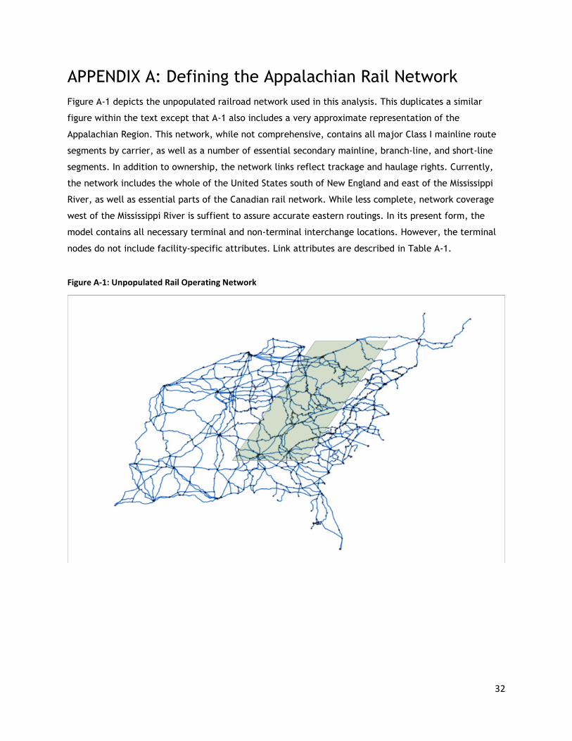
APPENDIX A: Defining the Appalachian Rail Network Figure A-1 depicts the unpopulated railroad network used in this analysis. This duplicates a similar

figure within the text except that A-1 also includes a very approximate representation of the

Appalachian Region. This network, while not comprehensive, contains all major Class I mainline route

segments by carrier, as well as a number of essential secondary mainline, branch-line, and short-line

segments. In addition to ownership, the network links reflect trackage and haulage rights. Currently,

the network includes the whole of the United States south of New England and east of the Mississippi

River, as well as essential parts of the Canadian rail network. While less complete, network coverage

west of the Mississippi River is suffient to assure accurate eastern routings. In its present form, the

model contains all necessary terminal and non-terminal interchange locations. However, the terminal

nodes do not include facility-specific attributes. Link attributes are described in Table A-1.

Figure A-1: Unpopulated Rail Operating Network

33

Table A-1 – Network Link Attributes

Attribute Description

LENGTH Link length CAPACITY Average number of trains under optimal conditions NO. OF RAILROADS Number of railroads with operating rights (ownership, trackage, haulage, etc.) RAILROADS NOS. AAR identifiers for each railroad with operating rights NO. OF TRACKS Number of mainline tracks FREE FLOW SPEED Maximum speed under optimal conditions TRAVEL TIME Link length / Free Flow Speed P1,P2 Capacity function parameters ML CLASS FRA Track Class LINK TYPE Based on usage - yard tracks, directional operations etc. SIGNAL CTC, ABS, Manual Block CAPACITY CODE Based on siding spacing, reverse signals, etc.

Unlike traditional highway traffic models, the rail assignment model considers multiple commodities,

with each commodity having a potentially different set of costs and priorities. The model also deals

with the subdivision of the overall railroad network into subnetworks for specific companies, with

transfers allowed only at designated points and at additional cost. The solution process identifies

network flow assignments that minimize the overall system transportation cost. This system

equilibrium approach is intended to replicate the behavior of railroad management as described above

and produce network link volumes and performance levels closely approximating actual observed

conditions.

34

APPENDIX B: Analytical Methodology, Assumptions, and Parameters

The modeling process involves several specific steps. These are enumerated, then discussed

individually in the text that follows. Process steps include:

1. Developing a fully functional railroad network that captures individual link capacities and which can accommodate observed railroad behaviors;

2. Assembling a largely disaggregated population of baseline railroad traffic;

3. Simulating the effects of reduced coal production on future traffic volumes;

4. Developing operating cost parameters by traffic type;

5. Flowing the baseline traffic over the current rail network based on cost-minimizing behaviors;

6. Flowing scenario traffic over the same baseline network; and

7. Comparing optimal baseline and scenario traffic flows to identify specific railroad route segments that may be made vulnerable by declining coal traffic.

The Model Setting Section 4 (p. 27) of the March 2017 ARC document cited in the main report carefully describes the

process through which railroads make infrastructure decision. However, as a quick review, there are

four points worth repeating.

1. Railroads operate networks where geographically dispersed origin-destination pairs often share common route segments. Very simply, this means that what happens at a seemingly removed location can have network effects in many different places. Theoretically, this network interdependence ties all network decision-making into one very large problem.

2. To a point, railroad routes are characterized by economies of density, whereby the unit cost for each shipment is lowered by the presence of additional traffic.

3. Railroad infrastructure is extremely long-lived. Many assets have lives that can be readily extended to between 50 and 100 years. Moreover, most of the costs associated with infrastructure development are sunk, meaning they are not recoverable if the railroad chooses to abandon service.

4. In North America, railroad infrastructure is privately owned. Historically, jurisdictions exchanged rights of way for the railroads’ willingness to fulfill common carrier obligations, but the property and improvements belong to the railroads, so that public-sector input is often limited.

Again, theoretically, decision-making in this sort of network setting requires the solution of a complex

network optomization problem, where capital, maintenance, and operating costs are balanced against

the stream of expected revenues tied to each route segment

In practice, the data and forecasts needed to solve this complex problem over a 30-50 year timespan

do not exist. Thus, as a second-best alternative, senior railroad industry managers typically develop

35

shorter-run operating plans that treat network extent and configurations as largely fixed. Railroads

revisit network issues only periodically, when network capacities limit new, long-run business

opportunities or when they impose clearly avoidable long-run costs. These periodic evaluations—as they

pertain to changing coal traffic—are what is modeled here.

Baseline and Scenario Traffic Data Baseline traffic data were developed through the use of the Surface Transportation Board’s 2011

Carload Waybill Sample (CWS). The baseline year is 2011 because it was the year in which aggregate

railroad industry coal revenues peaked and the last year in which coal volumes were near their historic

highs.15

Traffic volumes, measured in both tons and carloads, were aggregated, based on originating railroad,

origin county, destination county, and commodity category. In addition to shipment volumes, the CWS

data were also used to determine average shipment distance, average revenue tons-per-carload,

average car tare weights, and the average number of interchanges associated with each record.

Information for “off-network” railroad movements were excluded from the data.

Commodity group definitions were developed to reflect cost differences associated with differing

equipment types, commodity values, and operating requirements, while at the same time keeping the

number of observations at a manageable level. Commodity definitions, based on corresponding two-

digit Standard Transportation Commodity Codes (STCCs), are provided in Table B-1. Summary statistics

for the resulting data set are provided in Table B-2.

The 2011 baseline data were used to create the scenario dataset that reflects the 2036 coal production

forecasts. For non-coal commodities, we did not attempt to forecast future traffic volumes. For coal

movements originating in the eastern U.S., the data were adjusted to reflect the predicted 2036 values

as described above, in Table B-3. Importantly, the rail traffic to, from, and within the study region

includes coal mined in regions outside Appalachia (e.g., the Illinois basin or the Powder River basin).

Based on EIA production forecasts, we assumed that production in those non-Appalachian regions would

remain constant over the 20-year time horizon.16

15 Industry-wide, railroad coal volumes peaked in 2007. See, Association of American Railroads, Annual Statistics of Class I Railroads, 1978 – 2015. 16 See U.S. Department of Energy, Energy Information Administration, Annual Energy Outlook: 2017, Supplemental Tables, “Coal Supply, Disposition, and Prices,” https://www.eia.gov/outlooks/aeo/data/browser/#/?id=15-AEO2017&cases=ref2017&sourcekey=0

36

Table B-1 – Commodity Group Definitions

Study Commodity Group Corresponding Two-Digit STCCs

1 Grain 01, 08, 09 2 Low-Value Bulk 10, 14, 29, 32, 40 3 Coal 11 4 Chemicals and Petroleum 13, 28 5 Manufactured Products 19-27, 31, 33-39 6 Other (Intermodal) 41-47 99 Empties

Source: Center for Transportation Research

Table B-2 – Baseline Traffic Summary Statistics

Commodity Group

Number of Records

Average Shipment Distance

Average Revenue Tons per Carload

Average Car Tare Weight

Average Number of Cars per Record

Total (Expanded) Tons

1 2,892 926 94 34 377 91,276,492 2 7,011 824 87 36 336 212,816,277 3 1,045 585 115 26 5,321 663,689,327 4 8,421 926 88 36 224 160,798,924 5 14,720 1,056 71 39 397 260,174,517 6 1,831 1,578 16 74 4,710 108,573,822

Source: Center for Transportation Research

Table B-3 – Coal Scenario Annual Coal Output (Tons in Millions)

Year Alabama Eastern Kentucky Maryland Ohio Penn. Tenn. Virginia

Northern WV

Southern WV

2011 19.07 67.93 2.94 28.17 59.18 1.55 22.52 41.85 92.81 2012 19.32 48.80 2.28 26.33 54.72 1.09 18.97 41.49 78.94 2013 18.62 39.50 1.93 25.11 54.01 1.10 16.62 42.39 70.40 2014 16.36 37.39 1.98 22.25 60.91 0.84 15.06 48.86 63.33 2015 13.19 28.10 1.92 17.04 50.03 0.90 13.91 47.79 47.85 2016 9.12 16.88 1.58 12.58 45.85 0.67 12.79 43.50 36.50 2017 8.95 16.41 1.75 12.87 52.73 0.66 15.04 48.94 39.44 2018 9.29 16.94 1.74 12.33 51.81 0.68 15.53 48.60 40.73 2019 9.94 17.11 1.74 12.47 52.39 0.70 15.68 48.66 41.13 2020 10.24 17.12 1.75 12.92 54.25 0.71 15.69 48.88 41.15 2021 10.55 16.83 1.70 12.58 52.86 0.71 15.43 49.07 40.46 2022 10.88 16.60 1.87 12.82 52.86 0.72 15.21 49.15 39.90 2023 11.19 16.15 1.80 12.36 50.96 0.73 14.81 49.40 38.83 2024 11.52 15.77 1.79 12.28 50.63 0.73 14.45 49.41 37.90 2025 11.85 15.45 1.78 12.21 50.32 0.74 14.16 49.40 37.14 2026 12.18 15.04 1.77 12.15 50.10 0.75 13.79 49.41 36.16 2027 12.54 14.66 1.80 12.37 50.98 0.76 13.43 48.99 35.23 2028 12.92 14.33 1.77 12.15 50.07 0.76 13.14 48.89 34.46 2029 13.23 14.02 1.69 11.61 47.87 0.77 12.85 48.77 33.69 2030 13.49 13.79 1.65 11.35 46.78 0.77 12.64 48.71 33.15 2031 13.70 13.60 1.66 11.39 46.94 0.78 12.46 48.83 32.68 2032 13.93 13.44 1.70 11.69 48.20 0.79 12.32 48.78 32.32 2033 14.16 13.33 1.68 11.52 47.49 0.80 12.22 48.72 32.05 2034 14.38 13.23 1.62 11.11 45.82 0.79 12.13 48.62 31.80 2035 14.59 13.14 1.63 11.19 46.14 0.80 12.05 48.51 31.60 2036 14.78 13.06 1.64 11.29 46.55 0.81 11.97 48.38 31.40

Source: West Virginia University

37

Cost Parameters Based on the optimization process (described below), it was necessary to develop operating cost

parameters for individual railroads and specific commodity groups. With the help of the Association of

American Railroads (AAR), these data were constructed from the STB’s annual R-1 operating and

financial data as reported in AAR documents.

The available data report information for each of the seven Class I railroads, as well as aggregated

values for eastern and for western railroads. They do not provide information pertaining to short-line

operations or costs. The eastern railroad aggregations were used as a basis for determining short-line

data. However, where possible, short-line data were modified to reflect information from other

sources.

38

APPENDIX C: An In-Depth Description of RAILNET The purpose of the algorithm is to provide an analytical framework for realistically predicting traffic

patterns within the rail network and for evaluating the effects of these flows on capacity. The model

allows the study of congestion effects in the railroad system. The analyst may formulate and explore

outcomes under differing traffic and network scenarios. Origin-destination (O-D) demand patterns for traffic (e.g., the traditional traffic generation and distribution steps) are generated externally and may

reflect a variety of user interests.

Unlike traditional highway traffic models, the rail assignment model must consider multiple

commodities, with each commodity having a potentially different set of costs and priorities. The model

must also deal with the subdivision of the overall railroad network into subnetworks for specific

companies, with transfers allowed only at designated points. The solution hypothesizes a network flow

assignment that minimizes the overall system transportation cost. This system equilibrium approach

should replicate the behavior of railroad management as described above and produce network link

volumes and performance levels closely approximating actual observed conditions.

System equilibrium (SE) formulations for freight modeling—like the formulation used here—are now

routine. In the 1970s, Dafermos formulated an SE assignment model for examining multiclass flow

problems, which included multi-commodity freight flow assignments.17 Friesz et al. describe the use of

a multi-commodity freight network equilibrium model that specifically attempts to reconcile the user-optimized (shipper) and system-optimized (carrier) aspects of the freight flow problem.18 This model

performs a combined distribution, mode split, and assignment from the shipper standpoint. The

resulting origin-destination flows and generalized routes provide inputs to a carrier submodel. This

module computes system equilibrium flows for each mode/carrier. This model, while broader in scope

than needed for this study, nevertheless contributes many useful ideas. Subsequent works by

Harker; Crainic, et al.; and Guélat et al. further explore the theory of SE freight flow

assignment.19

Design Criteria and Objectives The objective of the model is to predict, given a matrix of commodity flows between origin and

destination pairs, the likely volume of flow on each link in a rail network. The flow patterns should

17 See Dafermos, Stella C., “The Traffic Assignment Problem for Multiclass-User Transportation Networks,” Transportation Science, 1971, pp. 73-87. 18 Friesz, Terry L. et al., “The Northeast Regional Environmental Impact Study: Theory, Validation and Application of a Freight Network Equilibrium Model.” Report ANL/ES-120 prepared by Argonne National Laboratory, Argonne, Ill. for U.S. Department of Energy, 1981. 19 See Harker, Patrick T., “Predicting Intercity Freight Flows,” VNU Science Press, Utrecht, The Netherlands, 1986; Crainic, T.G., Florian, M., and Léal, J., “A Model for the Strategic Planning of National Freight Transportation by Rail.” Transportation Science, vol. 24, no. 1, 1990, pp. 1-24; and Guélat, J., Florian, M., and Crainic, T.G, “A Multimode Multiproduct Network Assignment Model for Strategic Planning of Freight Flows,” Transportation Science, vol. 24, no. 1, 1990, pp. 25-39.

39

accurately reflect the underlying decision logic used by shippers and railroad managers in routing

traffic. Given a flow volume and a service function for each facility, the average travel time, and thus

delay, can be calculated for that facility.

The model is intended to provide a strategic view of network flows, rather than a tactical or operating viewpoint. To this degree, individual train operations are not replicated, nor are the flows considered

in terms of traffic blocks which could be used for operations planning. The statistics provided represent

average characteristics of the system. Peaking, traffic disruptions, and other transient phenomena are

not addressed.

It is assumed that the network is fixed and that no improvements are made that would affect traffic

flows. The analyst may, of course, use the model to test hypothetical improvements. These network

changes must be specified exogenously, however. The model formulation reflects:

1. The flow of multiple separate commodity classes, each having a distinct rate structure;

2. The network topology of the modeled railroad system, including line haul arcs, terminals, and transfer points;

3. Corporate ownership of network elements;

4. Service characteristics of various network elements, such as line haul links and terminals; and

5. Restrictions on the movement of commodities over specific carriers or network elements as needed to reflect operational practice.

Carriers and Shippers

We assume that the transportation market consists of a set M of transportation providers or carriers

)( Mm∈ . In this study, the carriers are railroads, although, in general, this is not a requirement. The

set M may include carriers representing other modes of transportation, with appropriate adjustments

to the physical network and cost attributes.

Carriers are assumed in the model to be cost-minimizing entities. In economic terms, the firms are cost

efficient. The carriers supply services, singly or in concert, between various origin-destination (O-D)

pairs. An origin or destination may be a physical node in the network or an abstract node representing a demand centroid. This choice is left to the analyst. In general, however, because of the strategic

planning orientation of the model, demand nodes represent centroids of mass for some shipper

community in a region.

To reflect shipper demands, the construct contains a set W of O-D pairs. Some volume of a commodity

or commodities flows between each O-D pair w in W. We denote the set of commodities as P, with p

denoting an individual commodity. A commodity may represent a product, as in coal or grain, or a

specific type of service, such as intermodal transportation. Empty cars returning to the point of loading may

also be modeled as a commodity. It is assumed that each commodity has distinct cost characteristics.

The demand for transportation is fixed exogenously. Via measurement or some external procedure such

as trip distribution or an input-output type model, the volume of flow for each commodity between

each O-D pair is determined and provided as an input to the model. The model does not, therefore,

40

replicate the decision making process of shippers in selecting markets for goods based upon economic

principles.

The matrix of flow quantities between all O-D pairs is designated Q, with submatrix Qp denoting the

flow of commodity p. For consistency, units for all flows in Q are specified in a measure of weight,

normally tons or metric tons. All flow values must be non-negative.

Links, Nodes, and the Complete Network

In scale, the modeled transportation network represents a region or nation. The topology of this

network describes the physical transportation network with little aggregation or abstraction.

Define L to be the set of all links in the network. For the most part, these links represent physical

transportation facilities such as line haul track segments and classification yards or terminals. We may, in certain cases, add abstract links as in the case of a demand centroid connector. Associated with

each link is a vector of attributes defining its physical and service characteristics.

In general, links in the real world network are undirected. For reasons which will become clear as the

formulation proceeds, we represent the network as a set of N nodes and A directed arcs. Each

undirected link is represented equivalently as a set of directed forward and reverse arcs.

There is no restriction against carriers sharing a physical link Lljil ∈= ),;( , as in the case of joint

track or trackage rights in the railroad industry. So that we can model each carrier individually, we

wish for the subnetworks to maintain separate representations for such shared physical facilities. The

forward arc representing link l for carrier m is then specified as a i j m l= ( , , ) . There may also be a

corresponding reverse arc ),,( mija l=′ . The subscript accounts for the case where we have parallel

physical arcs between i and j.

Each link l is represented, therefore, in the network by a set of forward arcs ),,( mjiA lMmF ∪= ∈ . If the

link is undirected, then there is a corresponding set of reverse arcs ),,( mijA lMmR ∪= ∈ .

Nodes in the model physically represent junctions between line segments or locations where line

characteristics change, as from single to multiple track. Nodes may also represent sources or sinks for

traffic flow.

Connections between carrier subnetworks take place at a set T of designated transfer locations. The

network is intermodal if transfers exist between carriers of different modes. Given a node

}{ NNt nm ∩∈ , the transfer between carriers m and n at this node may be designated as t nm , .

Transfers are directed, and for transfer t nm , , its counterpart t mn, may or may not be defined.

Henceforth, we will use the designation t without subscripts to refer to an individual transfer.

In this model, transfers have a vector of cost attributes, but are assumed not to have capacity

constraints or to experience congestion effects. If transfer congestion effects are desired, the network

41

structure can be modified by adding logical links through which flow to the transfer point must pass.

We assume otherwise that carriers provide line haul service as necessary to handle transfer flows.

The complete network is therefore represented by ),( ANG = , where N is the set of nodes and A is the

set of directed arcs which connect these nodes. The arcs represent the set of L physical and logical

links. Each carrier m operates a subnetwork Gm which consists of Nm nodes and Am directed arcs.

The complete network therefore consists of the union of the carrier subnetworks, with NN mMm∪= ∈

and AA mMm∪= ∈ . The set T of transfers defines connections where flows may pass between the

subnetworks. We see that, in general, subnetworks may share nodes, as at transfers, but arcs are

unique to a carrier. In other words, nmAA nm ,},{ ∀∅=∩ .

Commodity Flows

The volume of commodity p on arc a is given by vpa . Likewise, the volume of commodity p through

transfer t is vpt . Both vp

a and vpt must be non-negative. The vector of network facility volumes for

commodity p is:

∈

∈=

Ttv

Aavv p

t

pap

),(),(

.

The complete facility loading in the network, called the load pattern, is given by vector ).,( Ppvv p ∈=

Next, we derive a relationship between path flows and arc/transfer flows. For a given O-D pair, w, the

volume of commodity p flowing between w is Qqq ppw

pw ∈, . Define Kw as the set of paths through the

network connecting w. If, for w, i is the origin node and j is the destination node, a path Kkk www ∈, ,

can be expressed as:

),,,,,,,,,,,,( 121121 jnntnntnnik uussw KKK ++= .

Here, nx represents an ordinary node in the chain and yt represents a transfer. Alternately, the path

may be expressed as a chain of arcs:

().),,(,),,,(),,,(),,,(

,),,,(),,,(),,,(,),,,(,),,(

33132221

212111112111

mjnmnnmntmtnmnnmntmtnmnnmnik

zuuuuu

ssssw

++−

+−=K

KK

Path wk can be seen to consist of several subpaths, each of which belongs to a specific carrier:

42

( )( )( ).),,(,),,,(),,,(

,),,(,),,,(),,,(,),,(,),,,(),,,(

,

33132

2212121

11112111

3

2

1

321

mjnmnnmntkmtnmnnmntk

mtnmnnmnikkkkk

zuuuumw

usssmw

smw

mw

mw

mww

++

−+

−

=

=

=

++=

KK

K

Denote the flow of commodity p on path wk as wkpτ , which must be non-negative. To assure flow

conservation, the flows of p on all paths in wK must sum to the total specified flow volume of p

between O-D pair w:

qpwKk

pkww w=∑ ∈ τ . (1)

The set of all paths between all O-D pairs over which commodity p might flow is KK wWw∪= ∈ . The

relationship between arc flows and path flows for p is expressed as:

τδ pkKk

ka

pav ∑= ∈ (2)

where: δ ka =

otherwise. 0 path in is arcif 1 ka

The equivalent relationship between transfer flows and path flows is:

τδ pkKk

kt

ptv ∑= ∈ (3)

where: δ kt =

otherwise. 0 path in is transferif 1 kt

Note that for a particular path kw , the total flow is the vector ),,,( 21 ττττ pkkkk wwww

K= which contains a

flow (possibly zero) for each commodity. The indexed set { }Kkk ∈≡ ,ττ contains all path flows in the

network. This set is called the flow pattern. The equivalent load pattern for arcs and transfers is

constructed using the relationships in (2) and (3). The load vector for arc a is ),,,( 21 vvvv paaaa K= and

for transfer t is ),,,( 21 vvvv ptttt K= . The load pattern is then the indexed set { } { }TtvAavv ta ∈∪∈≡ ,,

, which is a restatement of the earlier definition.

Costs and Flow/Cost Relationships Given a pattern of flows, we are now interested in determining the cost characteristics of those flows.

The cost of a flow pattern is equivalent to the cost of the corresponding load pattern. Thus, we may

look at costs for loads on individual facilities.

43

Average Costs

The average cost of a flow unit of commodity p on arc a is given by aps and on transfer t by sp

t . Both

spa and sp

t must be non-negative. The vector of network average facility unit costs for commodity p is:

∈

∈=

Tts

Aass p

t

pap

),(),(

.

Vector ),( Ppss p ∈= provides the average unit costs for all facility/commodity combinations.

For a given commodity, the unit cost on a facility is normally considered to be a function of the load

pattern. In general, we therefore can say that )(vss aa = and )(vss tt = . Realistically, however, it can

be questioned whether, for example, there are cost interactions between arcs or transfers representing

different physical facilities. In our model, therefore, we assume:

a) The cost functions for a given transfer are not affected by the flows at other transfers or by arc

flows. This infers that flows at m nt , do not interact with flows for t mn,

b) The cost function for an arc is not affected by transfer flows; and

c) The cost function for an arc is only affected by flows on arcs which represent the same physical link. There is no interaction between flows on separate physical links.

The real world railroad system behaves similarly.

Under assumption (c), the cost function for an arc can be affected by the flows on other arcs

representing the same physical facility. The interaction between flows is apparent, for example, on a

single track railroad line represented in the model by a forward arc and a reverse arc. The delay

characteristics for such a line are a function of the total traffic in both directions. We then define A

as a set of interacting arcs representing a physical link, l = (i; j), l ∈ L, connecting nodes i and j. In

general, for most railroad line classes where two-way traffic interacts, AAA RF ∪= . In the case of

non-interacting two-way traffic, as with directional double track, AA F= if Aa F∈ , otherwise

AA R= . It is apparent then, for arc flows, that we must evaluate a portion of the load pattern defined

as { }., Aavv aA ∈≡

Based upon the above assumptions, and the definition of A , the form of the average cost function can

be made more specific for each facility type. The average cost vector for arc a is now )(vss Aaa = .

Since each commodity can have a distinct cost structure, the vector equation may be expressed as a

set of p-scalar equations:

44

).,,(

),,,(

1

111

vvss

vvss

pAA

pa

pa

pAAaa

KM

K

=

=

Transfers have no interaction, and therefore, no equivalent to A . The average cost vector for transfer

t is )(vss ttt = , with the corresponding set of p-scalar equations:

).,,(

),,,(

1

111

vvss

vvss

ptt

pt

pt

ptttt

KM

K

=

=

Total Costs

The preceding section defined average cost relationships to the flow pattern. The total cost for the

flow pattern is the practical measure of interest, however. As with the average unit cost, the total cost

can be expressed in terms of the facility load pattern. The total cost for the flow of commodity p on

arc a is vvs paA

pa )( . The corresponding total cost for a transfer t is vvs p

ttpt )( . The total cost of the flow

for product p is then:

.)()(∑ ∑+∈ ∈Aa Ttptt

pt

paA

pa vvsvvs (4)

The total system cost for the entire load pattern is:

( ).)()(∑ ∑ ∑+∈ ∈ ∈Pp Aa Ttptt

pt

paA

pa vvsvvs (5)

Facility Cost Functions

To compute costs, specific average cost functions which adhere to the requirements of the previous

section are needed. These functions yield a generalized cost expressed as cost per unit of weight. First

the case of arcs is examined and then that of transfers.

Arc Cost Functions

In this model, the average cost function applies to arcs which model line-haul track segments.

Line-haul cost function

The line haul average cost function is hypothesized to provide a generalized cost having a weight-

distance based component and a time based component. The function has the form:

hfvTlmvs pa

paAAA

paA

pa )()( += (6)

45

where: mpa = the cost per net ton-mile for commodity p on arc a;

lA = the length of the arc’s physical link;

hpa = train cost per hour for commodity p on arc a;

)(vT AA = travel time on arc a, given load pattern vA ;

f pa = commodity conversion factor, weight to trains.

Subsequent sections discuss these terms and their explanatory variables.

Weight-distance cost term

The weight-distance component lm Apa reflects cost elements such as track maintenance, equipment

wear, allocated overhead costs, etc. Such items are normally measured as a cost per net or gross ton-

mile of carriage. We use the A subscript on the length variable to denote a link specific attribute.

Given a gross-weight to payload ratio, mpa can be adjusted quite easily to reflect the gross ton-mile

cost. We assume that the mileage based coefficients are constant over all flow volumes.

Time cost term

The second component of the cost function is the time cost of transporting the commodity over the

arc. This term accounts for costs such as fuel, labor, time value of locomotives and equipment, and

time value of the commodity being transported. These cost categories are measured in cost per unit

time, typically dollars per hour. The discrete unit of many of these costs is the train, and travel time

over a line segment is typically viewed on a per-train basis.

The travel time is, of course, a direct function of the total volume, in trains, on the link. If the load

pattern vA can be converted to the equivalent number of trains, a congestion function can be used to

compute the average link travel time. To do this, we define for each commodity p and arc a, a factor

f pa which converts the net weight of p to a number of equivalent trains:

αχωεω

apm

pm

pm

pmp

af+

= (7)

where: Aa m∈

ωpm = weight of commodity p in a loaded car for mode m;

ε pm = tare weight of an empty car for commodity p on mode m;

χ pm = trailing gross weight of a train of commodity p on mode m;

α a = calibration factor for arc a.

The number of trains V pa on arc a of commodity p is then vf p

apa . The total number of trains, AV ,

defined by load pattern Av , is

46

vfV paPp Aa

paA ∑ ∑= ∈ ∈ . (8)

This approach is similar to that employed by Crainic, Florian, and Léal, who report good agreement

with observed volumes on Canadian railroads.

There are several points related to this approach which should be noted. First, equation (8) yields, in

general, a non-integer number of trains. Since we are considering average flow, and not modeling detailed operations, this is acceptable. Second, the trailing gross weight of a particular train type does

not include locomotive weights. Third, the arc calibration factor aα is used to adjust train weights on

arcs representing links with operating restrictions, such as grades or short sidings, which do not permit

operation of the “average” train. It may also be used to increase weights. Finally, for a given product

p, values of ω and ε are recommended to be constant for carriers which interchange traffic.

Different values may be appropriate where transloading takes place at a transfer point. Otherwise,

there will be a flow imbalance in terms of cars at transfer points, although weight flow conservation

constraints will not be violated.

Given a congestion function, the average travel time T A for the arc can be determined as a function

of the train volume V A . Since V A is, in turn, a function of the load pattern vA , then )(vTT AAA = . In

formulating our assignment model formulation, we may use, in general, any congestion function. The solution procedure requires the congestion function to meet certain criteria. These will be discussed in

a later section of the paper.

The time cost term needs to be expressed in terms of cost per unit weight. The product of hvT paAA )(

has units of cost per train-hour. Multiplying this by f pa will yield units of cost per unit weight. The

complete cost term is, therefore, hfvT pa

paAA )( .

Transfer Cost Function

In this model, transfer locations have no congestion effects or capacity limits. The cost model for a

transfer is designed simply to reflect a commodity specific cost per car for performing the transfer:

fmsp

tpt

pt

~~= (11)

where: mpt~ = the cost per car of commodity p using transfer t;

fp

t~ = cars per ton of commodity p using transfer t.

The cost tpm~ may reflect factors such as an average time cost for the transfer, administrative charges,

or delivery costs.

47

Railroad routing practice usually minimizes the number of transfers, since a transfer normally

represents delay to the shipment. Of the set of transfer points available to a large railroad, historic

traffic patterns will favor a subset for the majority of interchange activity. Other interchanges will have relatively little traffic. If the predicted flow pattern is to replicate actual conditions, the transfer

cost function should reflect this hierarchy.

Objective Function

The preceding sections provided a framework for defining the network, describing demand and load

patterns, and defining costs for facility loadings. Of interest now is a mathematical expression which

will produce the load pattern in the network.

In this model, the objective is to select the load pattern that minimizes total generalized costs. The

use of generalized costs reflects total logistics costs, and, in an environment of competition, carriers

and shippers will, it can be argued, work together to minimize total costs. Since the model is based

upon fixed demands, the shippers are not explicitly included as agents. The generalized cost may, however, contain components, such as the time value of commodities, to implicitly represent shipper

interests. These cost components decrease the utility of routes with poor service characteristics. From

a carrier standpoint, since the time frame of the model is short term, rates are assumed to be fixed. By

minimizing costs, a carrier will maximize the portion of revenue brought to the bottom line.

Mathematical Program

The load pattern at which total generalized costs are minimized is called the system optimum (SO).

Mathematically, the SO load pattern can be determined using the following non-linear program:

( )∑ ∑ ∑+= ∈ ∈ ∈Pp Aa Ttpt

pt

pt

paA

pa vvsvvsZ )()(min (12)

subject to:

wpqpwKk

pkww w

,,∀=∑ ∈ τ (1)

Kkwp wwpkw

∈∀≥ ,,,0τ (13)

pav pkKk

ka

pa ,,∀∑= ∈ τδ (2)

ptv pkKk

kt

pt ,,∀∑= ∈ τδ . (3)

The constraints (1) and (13) assure flow conservation on paths. Constraints (2) and (3) transform path

flows into arc and transfer flows.

Necessary and Sufficient Conditions

The solution of the above problem will yield the desired SO flow pattern for the network provided that

certain necessary and sufficient conditions are met. Convexity of the feasible region is guaranteed by

the fact that constraints (1), (2), and (3) are linear equalities. A second requirement is that equation

48

(12) be convex. This can be guaranteed if all of the arc and transfer performance functions are convex,

positive, and monotone increasing, and, therefore, the product vvs paA

pa )( is convex over the range of

flows vpa . The objective function will then be convex since the sum of a series of convex functions is

itself convex. The mathematical conditions are defined in the following sections.

Necessary Conditions

The necessary conditions, which can be found in a number of texts, such as Sheffi20, are as follows:

Kkwpcc wwpw

pk

pk ww

∈∀=− ,,,0)( )τ (14)

and

Kkwpcc wwpw

pkw

∈∀≥− ,,,0). (15)

Equations (1) and (13), the flow conservation constraints, must also be met.

Variable cpkw represents the marginal total cost for moving product p over path kw :

τ∂∂

pk

pk

w

w

Zc = . (16)

The marginal cost, well known in economic theory, is the addition to total costs of adding an additional

incremental unit of commodity p to the flow on path kw . The marginal cost for commodity p on path

wk is then

∑+∑= ∈∈ Ttpt

ktAa

pa

ka

pk ccc ww

w δδ

where δ ka

w and δ kt

w are indicator variables as in equations (2) and (3).

Variable c pw

) is the dual variable for the corresponding constraint in equation (1). According to the

duality theory of linear programming, this dual variable is the cost of adding an increment of

commodity p to the total flow between O-D pair w. Thus, c pw

) is also a marginal cost. From equation

(14), for O-D pair w flow of commodity p on path Kk ww∈ is non-zero only when cc pw

pkw

)= . Paths

where wkpc is greater than the associated dual c p

w)

receive no flow.

20 Sheffi, Yosef. Urban Transportation Networks: Equilibrium Analysis with Mathematical Programming Methods. Englewood Cliffs, NJ: Prentice-Hall, Inc, 1995.

49

Although the marginal costs are herein expressed in terms of paths, equivalent arc and transfer

formulations are easily derived. Facility marginal costs are discussed in detail in a subsequent section

of the paper.

Sufficient Conditions

The condition for the existence of a unique minimum to the multi-commodity SE problem is that the

objective function be strictly convex. If the Hessian of Z (the matrix of second derivatives of Z) is positive definite, this is sufficient to demonstrate strict convexity, and, thus, the existence of a unique

minimum. The Hessian, H, is positive definite if, for 0,0 >≠ Hvvv T . In the formulation, elements of H

relating to arcs are positive, since arc cost functions will be strictly convex, positive, and monotone

increasing. Transfers, however, have a linear cost function which yields a second partial derivative of

zero. The reader can verify that, under these conditions, terms in HvvT contain only arc flows. By the

criteria applied to arc cost functions, then, HvvT cannot be non-positive and H must be positive

definite.

The properties of convex function addition can also prove the uniqueness of the result. We know that objective function is convex because the sum of convex functions is always convex. The objective

function in this program is the sum of strictly convex functions (arc costs) and convex functions

(transfer costs). If the result of the addition of convex and strictly convex functions is strictly convex,

then the program will guarantee a unique minimum.

Strict convexity requires that, given any two distinct points 1x and 2x ,

)()1()(])1([ 2121 xzxzxxz θθθθ −+<−+

for any value of θ θ, 0 1< < . Let f x( ) be a strictly convex function of x, and )(yf be a convex

function of y. Two sets of points, ),(11 yx and ),( 22 yx , contain distinct values of x and y. If the sum of

f x( ) and f y( ) is strictly convex, then

)]()()[1()]()([])1([])1([ 22112121 yfxfyfxfyyfxxf +−++<−++−+ θθθθθθ .

If f y( ) is convex, but not strictly so, then f y( ) must be linear on y, since ′′ =f y( ) 0 . It is

recognized, therefore, that

)()1()(])1([ 2121 yfyfyyf θθθθ −+=−+ .

These terms cancel in the inequality, leaving

)()1()(])1([ 2121 xfxfxxf θθθθ −+<−+

which we know to be true since f x( ) is strictly convex. Therefore, we have shown that the sum of

convex and strictly convex functions is strictly convex.

50

Since transfer flow cannot occur in the objective function without arc flow, the objective function

must always be strictly convex in the vicinity of the optimum, and, therefore, Z is a global minimum.

Solution Algorithm The mathematical program set forth can best be described as having a non-linear, multivariable, convex objective function with linear constraints. Solution approaches that provide insight into this

particular programs are provided in a number of references. In his text on network flows, Hu discusses

some of the unique issues associated with multi-commodity flow formulations, namely that the

constraint matrix is not unimodular and that the tremendous number of potential columns in the

solution algorithm hint at a column generation based solution procedure.21 Dafermos examines the multiclass assignment problem and proposes a two-stage solution procedure which has as its heart a

decomposition of the problem by class.22 Sheffi describes efficient two-stage algorithms for solving the

single commodity, non-linear SO problem which might be extended for the multi-commodity problem.

These include linear approximation procedures such as the Frank-Wolfe algorithm. Guélat, Florian, and

Crainic describe a solution procedure similar to Dafermos’ which is used in their network model.23

Algorithm Overview

The constraint set defines a convex polytope encompassing the feasible region. The heart of the

solution procedure is as follows. First, obtain an initial feasible flow pattern, v. This will represent a

point on the surface of the polytope. Then, with each step of the algorithm, find a new feasible

extreme vector, w, which improves the objective function. The two vectors v and w define a line in n-

space. Using a linear search procedure, find the value of θ which minimizes the convex combination of

v and w,

wvvnew θθ +−= )1( . (17)

The algorithm continues until vvnew ≈ .

The above procedure is generally referred to as a convex combinations algorithm. The important step

of determining the new feasible extremal vector w is the critical step. The procedure is to use the

gradient of the objective function to formulate a linear approximation to the objective function.

Minimizing this linear approximation to the value of the objective function subject to a system of linear

constraints has as its solution a corner of the feasible space. The objective function of this program is

)()()()(min vwvZvZwZ T−⋅∇+= . (18a)

21 Hu, T.C. Integer Programming and Network Flows. Reading, MA: Addison-Wesley Publishing Co, 1969. 22 Dafermos, Stella C. “The Traffic Assignment Problem for Multiclass-User Transportation Networks.” Transportation Science, 1971, pp. 73-87. 23 Guélat, J., Florian, M., and Crainic, T.G. A Multimode Multiproduct Network Assignment Model for Strategic Planning of Freight Flows. Transportation Science, vol. 24, no. 1, 1990, pp. 25-39.

51

Terms Z v( ) and ∇Z v v T( ) ( ) are constants that may be omitted. This results in the revised objective

function

wvvZ

wvZwZ ii i

T ∑

=⋅∇=∂∂ )(

)()()(min . (18b)

The term vvZ

i∂∂ )(

is simply the marginal cost with respect to vi . When the problem has the structure of

a network, a feasible optimal solution for equation (18b) may be found using a straightforward shortest

path algorithm.

In the multi-commodity flow problem, the vectors v and w are of dimension )( TAP + . By decomposing

the problem by commodity, the vector size may be reduced to )( TA+ , which represents a substantial

savings in computer storage. This approach was advocated in both the aforementioned papers by

Dafermos (1) and Guélat et al. (5). During each iteration of the algorithm, a linear approximation subproblem is solved for each commodity, using marginal costs with respect to the flow of that

commodity. Flows of the other commodities are held fixed.

We consider that, for the multi-commodity problem, the constraint coefficient matrix is not

unimodular. This means that, given integer flows for each commodity, optimal arc and path flows will

generally not be integer. In a strategic planning model such as this one, non-integrality of the solution

is not a problem, since quantities are generally large and the solution represents, at best, average

conditions.

Algorithm Description

The following paragraphs summarize the steps in the solution algorithm.

Step 0. Initialization Determine an initial feasible flow vector, v. This can be done using an iteration of

Step 1 with initial marginal costs corresponding to a zero flow state and θ = 1 for each commodity

subproblem.

Step 1. Flow Vector Update

For each commodity Pp∈ , perform the following sequence of steps:

a) Given v, compute marginal costs, cpa and cp

t , for all arcs Aa∈ and transfers Tt∈ .

b) For each O-D pair Ww∈ having a corresponding flow Qq ppw∈ , solve the shortest path

problem using cpa and cp

t as facility costs. Assign qpw to this path.

c) Let py be the load vector resulting from Step 1b, with y being the corresponding overall

load pattern. Using a one-dimensional search algorithm, solve the problem

)()()1(min yZvZ θθ +−

52

subject to: 10 ≤≤θ .

d) Let yvv ppp θθ +−= )1( .

Step 2. Stopping Criterion

The algorithm terminates if the iteration count exceeds a predetermined number or if the current

value of the objective function is within a predefined tolerance of the previous value. Otherwise,

return to Step 1.

Guélat et al. (5) prove that convex combinations algorithms which decompose the problem by

commodity will converge when the objective function and constraints are convex.

Marginal Cost Functions

The solution algorithm uses functions to compute two types of costs: marginal total costs and average

total costs. Derivations for the marginal cost functions are now provided.

We have two types of facilities of interest: arcs and transfer nodes. In general, the marginal cost apc

for transporting product p on arc a is:

∑

∑ ∑++= ∈ ∈ ∈Pp Aa Tt

ptp

a

ptp

apa

pap

apa v

vvsv

vvsvsc

∂∂

∂∂ )()()( . (19a)

The equivalent function for transfer facility t is:

∑

∑ ∑++= ∈ ∈ ∈Pp Aa Tt

ptp

t

ptp

apt

pap

tpt v

vvsv

vvsvsc

∂∂

∂∂ )()()( . (19b)

In practice, the following simplifying assumptions can be made:

a) The cost function for a given transfer is not affected by the flows at other transfers or by arc

flows; b) The cost function for an arc is not affected by transfer flows; and

c) The cost function for an arc is only affected by flows on arcs which represent the same physical

link. There is no interaction between flows on separate physical links.

These do not seem to conflict with real world behavior of the railroad system.

We define A as the set of logical arcs representing a physical link, l = (i; j), l ∈ L, connecting nodes i

and j. Arc a = (i, j, m)l then represents a service of mode m using l. In general, l is an undirected link,

so that for each arc a = (i, j, m)l, there is a corresponding reverse arc á = (j, i, m)l. We may have any

number of modes using l, each represented by corresponding logical arcs. The set A is, therefore

53

{ }MmmijaormjiaAa ll ∈==∈ ,),,(),,(| .

The load pattern for A is denoted by vA .

If an arc Aa∉ , then by assumption (c), 0=v

spa

pa∂

∂ . This said, the marginal cost function for arcs can

be simplified to:

∑ ∑+= ∈ ∈Pp Aapap

a

Apa

Apa

pa v

vvsvsc

∂∂ )()( . (19c)

For transfers, the marginal cost becomes:

∑+= ∈Ppptp

t

tpt

tpt

pt v

vvs

vsc∂

∂ )()( . (19d)

We further assume, however, that transfers are uncapacitated using the rationale that railroads will

dispatch trains to handle interchange traffic as necessary. The capacities of the adjacent arcs will then

govern transfer volumes. This leads to the conclusion that 0=v

spt

pt∂

∂ and, therefore:

sc pt

pt = . (19e)

The total cost function forms were described previously without specific reference to the form of the

congestion function used to compute arc travel times. We now address the problem of deriving a working form of the arc marginal cost function. Arc travel time is, of course, a direct function of the

arc attributes and the total volume, in trains, on that link. We use a polynomial link travel time

function having the form:

++=

CVktkRT

A

AAAA

γ

211 (20)

where: RA = free flow travel time, hours, for arcs in A ;

k1, k2, = empirical constants;

V A = total daily train volume for arcs in A ;

C A = total capacity, trains per day, for arcs in A .

This polynomial link travel time function has the desirable properties of being continuous, convex, everywhere positive, monotone increasing, and twice differentiable. Furthermore, the same basic

54

polynomial form, with the appropriate selection of constants, can be used to estimate terminal delay

as a function of volume. This allows terminals to be modeled as a special class of link.

The total train volume over the link, i.e. the arcs in A , is:

vfV paPp Aa

paA ∑ ∑= ∈ ∈ . (21)

Substituting, the arc cost function then becomes:

∑ ∑+∑ ∑++= ∈ ∈

∈ ∈ C

vfkvfkhfRlms

A

Pp Aa

pa

pa

Pp Aa

pa

pa

pa

paAA

pa

pa

γ

211 . (22)

For a given arc a and commodity p , we are faced with the partial differentiation of this function

with respect to the volume vpa in computing the arc marginal cost. This may be done most easily by

considering the separate terms in the equation, as follows:

a) pAav

lmpa

Apa ,,0 ∈∀=

∂∂

;

b) pAav

hfRpa

pa

paA ,,0 ∈∀=

∂∂

;

c) pAaffhRkv

vfkhfRpa

pa

paAp

a

Pp Aa

pa

pa

pa

paA

,,1

1

∈∀=∑ ∑∈′ ∈′

′′

′′

∂

∂;

d) =

∑ ∑∈′ ∈′

′′

′′

v

C

vfkhfR

pa

A

Pp Aa

pa

pa

pa

paA

∂

∂

γ

2

pAaC

vfffhRkC A

Pp Aa

pa

pa

pa

pa

paA

A,,

1

2 ∈∀

∑ ∑∈′ ∈′

′′

′′

−γ

γ.

The full marginal cost equation for the arc, commodity combination then becomes:

+

∑ ∑+∑ ∑++= ∈ ∈

∈ ∈ C

vfkvfkhfRlmc

A

Pp Aa

pa

pa

Pp Aa

pa

pa

pa

paAa

pa

pa

γ

211

55

∑ ∑

∑ ∑+∑ ∑

∈ ∈

∈′ ∈′

′′

′′

−

∈ ∈ Pp Aa

pa

A

Pp Aa

pa

pa

pa

pa

paA

A

pa

Pp Aa

pa

pa

paA v

C

vffhfRCkvfhfRk

1

21

γ

γ. (23a)

We recognize that, from equation (21), Vvf ApaPp Aa

pa =∑ ∑∈ ∈ , the total train volume over the link. The

terms within the parenthesis in equation (23a) are then recognizable as the volume/capacity ratio for

the link. Rewriting equation (23a) yields:

+

+∑ ∑++=∈ ∈ C

VkvfkhfRlmcA

A

Pp Aa

pa

pa

pa

paAa

pa

pa

γ

211

∑ ∑

+∑ ∑∈ ∈

−

∈ ∈ Pp Aa

pa

pa

pa

paA

A

A

APp Aa

pa

pa

pa

paA vfhfR

CV

CkvfhfRk1

21

γγ

. (23b)

Further reorganizing the terms, we obtain:

+∑ ∑ +++=∈ ∈

])([1Pp Aa

pa

pa

pa

pa

paA

pa

paAa

pa

pa hhvffRkhfRlmc

∑ ∑+

∈ ∈

−

Pp Aa

pa

pa

pa

A

pa

A

A

A

ApaA vfhCh

CV

CVfRk

γγ 1

2 . (23c)

A final reorganization yields the working form of the equation:

+ ∑ ∑ +++=

∈ ∈Pp Aa

pa

pa

pa

pa

pa

paAa

pa

pa hhvfkhfRlmc )]([1

∑ ∑+

∈ ∈

−

Pp Aa

pa

pa

pa

A

pa

A

A

A

A vfhChCV

CVk

γγ 1

2 . (24)

Given that the specified forms of the arc and transfer cost functions, the objective function is strictly

convex and the algorithm will converge to a global minimum. If transportation firms exhibit economies

of density, however, average unit costs decline with increasing volume to a point, and then increase as the firm incurs additional costs for handling traffic. This well known U-shaped average cost curve is

convex, but not monotone increasing. In this case, the terms vvs paA

pa )( will not generally be convex,

and, therefore, the objective function will be non-convex. This means that the program solution will

not have a unique minimum. The algorithm may converge to a minimum, but there is no guarantee that

this is the global minimum. This aspect of the problem needs further examination. If we consider, however, that our network consists only of major routes, each having a reasonable volume of traffic,

we may apply only the increasing side of the cost function.

56

Shortest Path Algorithm Step 1b of the solution algorithm uses a shortest path algorithm (SPA) to solve the minimum marginal

cost path problem for each O-D pair 0 with >∈ qWw pw . For each iteration over a commodity, p, the

SPA finds candidate paths between origin-destination pairs for flow enhancement. The arc and transfer

costs used in the solution of these shortest path problems represent the sum of the current unit cost

and the marginal cost for p based upon (v).

A version of the standard Moore algorithm generates these paths. Modifications to the SPA account for

some unique requirements of the model structure. First, the algorithm produces paths which account

for the decomposition of the overall network into a series of carrier subnetworks connected at transfer

points. This is done using an arc-chain path rather than a node chain path. The arc-chain formulation

also simplifies path tracing during the arc loading process. Second, if flow qpw has a designated

originating carrier, the SPA must ensure that the path starts with this carrier.

57

APPENDIX D: Post-Processing Cost Calculations

The short-run and long-run cost calculations developed in Section 4 are calculated based on changes in

traffic density and estimated relationship between traffic density and unit costs. Traffic density along

individual route segments is a key determinant of freight rail transportation costs. From an analytical

perspective, density and economies of density are the spatial analogue of scale economies.

Consider a route segment of a specific length denoted as j that is used within a number of shipments, i

(i=1…n).24 Economies of density suggest that for any time period t:

𝐶𝐶�𝑄𝑄𝑖𝑖𝑖𝑖𝑖𝑖 < 𝐶𝐶�𝑄𝑄1𝑖𝑖𝑖𝑖� + 𝐶𝐶�𝑄𝑄2𝑖𝑖𝑖𝑖� + … 𝐶𝐶�𝑄𝑄𝑛𝑛𝑖𝑖𝑖𝑖� 𝑖𝑖=1

𝑛𝑛

subject to:

�𝑄𝑄𝑖𝑖𝑖𝑖𝑖𝑖 ≤ 𝐷𝐷𝑖𝑖=1

𝑛𝑛

where Q’s denote traffic quantities and D is a designed optimal traffic volume over route segment j

beyond which unit costs escalate rapidly as traffic volumes approach the absolute physical capacity of

the route segment. These relationships are depicted graphically in Figure D-1.

The STB cost data described in Section 4 include divisions by four density groupings. These are

summarized in Table D-1. Therefore, based on corresponding traffic data, it was possible to allocate

various cost elements to individual railroads, by density class and year. Data are available in this form

from 1987 forward. These data were used to estimate density-specific cost functions for each density

class that resemble the surface pictured in Figure D-1. These were then applied to the subject trackage

based on estimated densities both before and after the changes in coal traffic.

24 Note that these shipments may involve a variety of different commodities, customers, or diverse origin-destination pairs, so long as all shipments include j within the routing.

58

Table D-1 – Density Class Definitions

Density Class Gross Ton-Miles pre Route-Mile

1 Density > 20 Million GTM/Track Mile

2 Density < 20 Million & > 5 Million GTM/Track Mile

3 Density < 5 Million & > 1 Million GTM/Track Mile

4 Density < 1 Million GTM/Track Mile

Figure D-1 – Unit Costs and Link Densities

Based on the RAILNET computations, 45 network links with a total distance of 1,166 miles will see

traffic declines will move then from Density Class 1 to Density Class 2. However, in the short-run the

operating carriers would be unable to immediately modify the characteristics of the affected trackage.

Therefore, in the short-run, the carriers would be assumed to operate along the Density Class I cost

structure, well to the right of the design capacity of that trackage.

However, as conditions allow, carriers would be expected to re-scale the affected trackage so that

route characteristics are consistent with lower traffic densities, thereby, lowering unit costs. This

results in an estimated short-run, per-ton-mile cost of $0.114 and a long-run, per-ton-mile cost of

$0.051.